跳到论文正文
W Papers独立论文阅读器 arXiv:0905.0642 论文正文 计算阅读时间 · 0%
引用这篇论文根据当前论文元数据生成,正式投稿前建议核对。


License: arXiv.org perpetual non-exclusive license
arXiv:0905.0642v1 [math.ST] 05 May 2009

Simultaneous support recovery in high dimensions: Benefits and perils of block ℓ1/ℓ∞\ell_{1}/\ell_{\infty}-regularization

Sahand Negahban⋆ Martin J. Wainwright†,⋆
Department of Statistics†, and
Department of Electrical Engineering and Computer Sciences⋆
UC Berkeley, Berkeley, CA 94720

May 5, 2009

Technical Report,
Department of Statistics, UC Berkeley
Abstract

Given a collection of r≥2r\geq 2 linear regression problems in pp dimensions, suppose that the regression coefficients share partially common supports. This set-up suggests the use of ℓ1/ℓ∞\ell_{1}/\ell_{\infty}-regularized regression for joint estimation of the p×rp\times r matrix of regression coefficients. We analyze the high-dimensional scaling of ℓ1/ℓ∞\ell_{1}/\ell_{\infty}-regularized quadratic programming, considering both consistency rates in ℓ∞\ell_{\infty}-norm, and also how the minimal sample size nn required for performing variable selection grows as a function of the model dimension, sparsity, and overlap between the supports. We begin by establishing bounds on the ℓ∞\ell_{\infty}-error as well sufficient conditions for exact variable selection for fixed design matrices, as well as designs drawn randomly from general Gaussian matrices. Our second set of results applies to r=2r=2 linear regression problems with standard Gaussian designs whose supports overlap in a fraction α∈[0,1]\alpha\in[0,1] of their entries: for this problem class, we prove that the ℓ1/ℓ∞\ell_{1}/\ell_{\infty}-regularized method undergoes a phase transition—that is, a sharp change from failure to success—characterized by the rescaled sample size θ1,∞​(n,p,s,α)=n/{(4−3​α)​s​log⁡(p−(2−α)​s)}\theta_{1,\infty}(n,p,s,\alpha)=n/\{(4-3\alpha)s\log(p-(2-\alpha)\,s)\}. More precisely, given sequences of problems specified by (n,p,s,α)(n,p,s,\alpha), for any δ>0\delta>0, the probability of successfully recovering both supports converges to 11 if θ1,∞​(n,p,s,α)>1+δ\theta_{1,\infty}(n,p,s,\alpha)>1+\delta, and converges to 00 for problem sequences for which θ1,∞​(n,p,s,α)<1−δ\theta_{1,\infty}(n,p,s,\alpha)<1-\delta. An implication of this threshold is that use of ℓ1/ℓ∞\ell_{1}/\ell_{\infty}-regularization yields improved statistical efficiency if the overlap parameter is large enough (α>2/3\alpha>2/3), but has worse statistical efficiency than a naive Lasso-based approach for moderate to small overlap (α<2/3\alpha<2/3). Empirical simulations illustrate the close agreement between these theoretical predictions, and the actual behavior in practice. These results indicate that some caution needs to be exercised in the application of ℓ1/ℓ∞\ell_{1}/\ell_{\infty} block regularization: if the data does not match its structure closely enough, it can impair statistical performance relative to computationally less expensive schemes.11 1 This work was presented in part at the NIPS 2008 conference in Vancouver, Canada, December 2008. Supported in part by NSF grants DMS-0528488, DMS-0605165, and CCF-0545862.

1 Introduction

The area of high-dimensional statistical inference is concerned with the behavior of models and algorithms in which the dimension pp is comparable to, or possibly even larger than the sample size nn. In the absence of additional structure, it is well-known that many standard procedures—among them linear regression and principal component analysis—are not consistent unless the ratio p/np/n converges to zero. Since this scaling precludes having pp comparable to or larger than nn, an active line of research is based on imposing structural conditions on the data (e.g., sparsity, manifold constraints, or graphical model structure), and studying the high-dimensional consistency (or inconsistency) of various types of estimators.

This paper deals with high-dimensional scaling in the context of solving multiple regression problems, where the regression vectors are assumed to have shared sparse structure. More specifically, suppose that we are given a collection of rr different linear regression models in pp dimensions, with regression vectors   ​βi∈ℝp\makebox[0.0pt][l]{\hskip 2.08334pt\hskip 0.58333pt\rule[8.23611pt]{2.84009pt}{0.43057pt}}{\beta}^{\,i}\in\mathbb{R}^{p}, for i=1,…,ri=1,\ldots,r. We let S⁡(  ​βi)={j∣  ​βji≠0}S(\makebox[0.0pt][l]{\hskip 2.08334pt\hskip 0.58333pt\rule[8.23611pt]{2.84009pt}{0.43057pt}}{\beta}^{\,i})=\{j\,\mid\,\makebox[0.0pt][l]{\hskip 2.08334pt\hskip 0.58333pt\rule[8.23611pt]{2.84009pt}{0.43057pt}}{\beta}^{\,i}_{j}\neq 0\} denote the support set of   ​βi\makebox[0.0pt][l]{\hskip 2.08334pt\hskip 0.58333pt\rule[8.23611pt]{2.84009pt}{0.43057pt}}{\beta}^{\,i}. In many applications—among them sparse approximation, graphical model selection, and image reconstruction—it is natural to impose a sparsity constraint, corresponding to restricting the cardinality |S⁡(  ​βi)||S(\makebox[0.0pt][l]{\hskip 2.08334pt\hskip 0.58333pt\rule[8.23611pt]{2.84009pt}{0.43057pt}}{\beta}^{\,i})| of each support set. Moreover, one might expect some amount of overlap between the sets S⁡(  ​βi)S(\makebox[0.0pt][l]{\hskip 2.08334pt\hskip 0.58333pt\rule[8.23611pt]{2.84009pt}{0.43057pt}}{\beta}^{\,i}) and S⁡(  ​βj)S(\makebox[0.0pt][l]{\hskip 2.08334pt\hskip 0.58333pt\rule[8.23611pt]{2.84009pt}{0.43057pt}}{\beta}^{\,j}) for indices i≠ji\neq j since they correspond to the sets of active regression coefficients in each problem. Let us consider some examples to illustrate:

  • •

    Consider the problem of image denoising or compression, say using a wavelet transform or some other type of multiresolution basis [17]. It is well known that natural images tend to have sparse representations in such bases [27]. Moreover, similar images—say the same scene taken from multiple cameras—would be expected to share a similar subset of active features in the reconstruction. Consequently, one might expect that using a block-regularizer that enforces such joint sparsity could lead to improved image denoising or compression.

  • •

    Consider the problem of identifying the structure of a Markov network or graphical model [10] based on a collection of samples (e.g., such as observations of a social network). For networks with a single parameter per edge (e.g., Gaussian models [19], Ising models [25]), a line of recent work has shown that ℓ1\ell_{1}-based methods can be successful in recovering the network structure. However, many graphical models have multiple parameters per edge (e.g., for discrete models with non-binary state spaces), and it is natural that the subset of parameters associated with a given edge are zero (or non-zero) in a grouped manner. Thus, any method for recovering the graph structure should impose a block-structured regularization that groups together the subset of parameters associated with a single edge.

  • •

    Finally, consider a standard problem in genetic analysis: given a set of gene expression arrays, where each array corresponds to a different patient but the same underlying tissue type (e.g., tumor), the goal is to discover the subset of features relevant for tumorous growths. This problem can be expressed as a joint regression problem, again with a shared sparsity constraint coupling together the different patients. In this context, the recent work of Liu et al. [14] shows that imposing additional structural constraints can be beneficial (e.g., they are able to greatly reduce the number of expressed genes while maintaining the same prediction performance).

Given these structural conditions of shared sparsity in these and other applications, it is reasonable to consider how this common structure can be exploited so as to increase the statistical efficiency of estimation procedures.

There is now a substantial and relatively mature body of work on ℓ1\ell_{1}-regularization for estimation of sparse models, dating back to the introduction of the Lasso and basis pursuit [28, 5]. With contributions from various researchers (e.g., [7, 19, 29, 37, 3]), there is now a fairly complete theory of the behavior of the Lasso for high-dimensional sparse estimation. A more recent line of work (e.g., [31, 35, 22, 30, 36]), motivated by applications in which block or hierarchical structure arises, has proposed the use of block ℓa,b\ell_{a,b} norms for various a,b∈[1,∞]a,b\in[1,\infty]. Of particular relevance to this paper is the block ℓ1/ℓ∞\ell_{1}/\ell_{\infty} norm, proposed initially by Turlach et al. [31] and Tropp et al. [30]. This form of block regularization is a special case of the more general family of composite or hierarchical penalties, as studied by Zhao et al. [36].

Various authors have empirically demonstrated that block regularization schemes can yield better performance for different data sets [36, 22, 14]. Some recent work by Bach [1] has provided consistency results for ℓ1/ℓ2\ell_{1}/\ell_{2} block-regularization schemes under classical scaling, meaning that n→+∞n\rightarrow+\infty with pp fixed. Meier et al. [18] has established high-dimensional consistency for the predictive risk of ℓ1/ℓ2\ell_{1}/\ell_{2} block-regularized logistic regression. The papers [15, 21, 24] have provided high-dimensional consistency results for ℓ1/ℓq\ell_{1}/\ell_{q} block regularization for support recovery using fixed design matrices, but the rates do not provide sharp differences between the case q=1q=1 and q>1q>1.

To date, there has a relatively limited amount of theoretical work characterizing if and when the use of block regularization schemes actually leads to gains in statistical efficiency. As we elaborate below, this question is significant due to the greater computational cost involved in solving block-regularized convex programs. In the case of ℓ1/ℓ2\ell_{1}/\ell_{2} regularization, concurrent work by Obozinski et al [23] (involving a subset of the current authors) has shown that that the ℓ1/ℓ2\ell_{1}/\ell_{2} method can yield statistical gains up to a factor of rr, the number of separate regression problems; more recent concurrent work [9, 16] has provided related high-dimensional consistency results for ℓ1/ℓ2\ell_{1}/\ell_{2} regularization, emphasizing the gains when the number of tasks rr is much larger than log⁡p\log p.

This paper considers this issue in the context of variable selection using block ℓ1/ℓ∞\ell_{1}/\ell_{\infty} regularization. Our main contribution is to obtain some precise—and arguably surprising—insights into the benefits and dangers of using block ℓ1/ℓ∞\ell_{1}/\ell_{\infty} regularization, as compared to simpler ℓ1\ell_{1}-regularization (separate Lasso for each regression problem). We begin by providing a general set of sufficient conditions for consistent support recovery for both fixed design matrices, and random Gaussian design matrices. In addition to these basic consistency results, we then seek to characterize rates, for the particular case of standard Gaussian designs, in a manner precise enough to address the following questions:

  1. (a)

    First, under what structural assumptions on the data does the use of ℓ1/ℓ∞\ell_{1}/\ell_{\infty} block-regularization provide a quantifiable reduction in the scaling of the sample size nn, as a function of the problem dimension pp and other structural parameters, required for consistency?

  2. (b)

    Second, are there any settings in which ℓ1/ℓ∞\ell_{1}/\ell_{\infty} block-regularization can be harmful relative to computationally less expensive procedures?

Answers to these questions yield useful insight into the tradeoff between computational and statistical efficiency in high-dimensional inference. Indeed, the convex programs that arise from using block-regularization typically require a greater computational cost to solve. Accordingly, it is important to understand under what conditions this increased computational cost guarantees that fewer samples are required for achieving a fixed level of statistical accuracy.

The analysis of this paper gives conditions on the designs and regression matrix   ​B\makebox[0.0pt][l]{\hskip 2.05pt\hskip 0.0pt\rule[8.12498pt]{5.73494pt}{0.43057pt}}{B} for which ℓ1/ℓ∞\ell_{1}/\ell_{\infty} yields improvements (question (a)), and also shows that if there is sufficient mismatch between the regression matrix   ​B\makebox[0.0pt][l]{\hskip 2.05pt\hskip 0.0pt\rule[8.12498pt]{5.73494pt}{0.43057pt}}{B} and the ℓ1/ℓ∞\ell_{1}/\ell_{\infty} norm, then use of this regularizer actually impairs statistical efficiency relative to a naive ℓ1\ell_{1}-approach. As a representative instance of our theory, consider the special case of standard Gaussian design matrices and two regression problems (r=2r=2), with the supports S⁡(  ​β 1)S(\makebox[0.0pt][l]{\hskip 2.08334pt\hskip 0.58333pt\rule[8.23611pt]{2.84009pt}{0.43057pt}}{\beta}^{\,1}) and S⁡(  ​β 2)S(\makebox[0.0pt][l]{\hskip 2.08334pt\hskip 0.58333pt\rule[8.23611pt]{2.84009pt}{0.43057pt}}{\beta}^{\,2}) each of size ss and overlapping in a fraction α∈[0,1]\alpha\in[0,1] of their entries. For this problem, we prove that block ℓ1/ℓ∞\ell_{1}/\ell_{\infty} regularization undergoes a phase transition—meaning a sharp threshold between success and recovery—that is specified by the rescaled sample size

θ1,∞​(n,p,s,α)\displaystyle\theta_{1,\infty}(n,p,s,\alpha) :⁣=\displaystyle:\,= n(4−3​α)​s​log⁡(p−(2−α)​s).\displaystyle\frac{n}{(4-3\alpha)s\log(p-(2-\alpha)s)}. (1)

In words, for any δ>0\delta>0 and for scalings of the quadruple (n,p,s,α)(n,p,s,\alpha) such that θ1,∞≥1+δ\theta_{1,\infty}\geq 1+\delta, the probability of successfully recovering both S⁡(  ​β 1)S(\makebox[0.0pt][l]{\hskip 2.08334pt\hskip 0.58333pt\rule[8.23611pt]{2.84009pt}{0.43057pt}}{\beta}^{\,1}) and S⁡(  ​β 2)S(\makebox[0.0pt][l]{\hskip 2.08334pt\hskip 0.58333pt\rule[8.23611pt]{2.84009pt}{0.43057pt}}{\beta}^{\,2}) converges to one, whereas for scalings such that θ1,∞≤1−δ\theta_{1,\infty}\leq 1-\delta, the probability of success converges to zero.

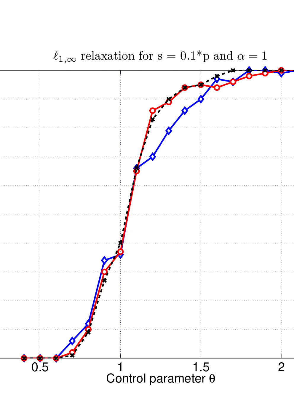
Figure 1 illustrates how the theoretical threshold (1) agrees with the behavior observed in practice. This figure plots the probability of successful recovery using the block ℓ1/ℓ∞\ell_{1}/\ell_{\infty} approach versus the rescaled sample size n/{2slog[p−(2−α)s}n/\{2s\log[p-(2-\alpha)s\}; the results shown here are for r=2r=2 regression parameters. The plots show twelve curves, corresponding to three different problem sizes p∈{128,256,512}p\in\{128,256,512\} and four different values of the overlap parameter α∈{0.1,0.3,0.7,1}\alpha\in\{0.1,0.3,0.7,1\}. First, let us focus on the set of curves labeled with α=1\alpha=1, corresponding to case of complete overlap between the regression vectors. Notice how the curves for all three problem sizes pp, when plotted versus the rescaled sample size, line up with one another; this “stacking effect” shows that the rescaled sample size captures the phase transition behavior. Similarly, for other choices of the overlap, the sets of three curves (over problem size pp) exhibit the same stacking behavior. Secondly, note that the results are consistent with the theoretical prediction (1):

Refer to caption
Figure 1: Probability of success in recovering the joint signed supports plotted against the rescaled sample size θLas:=n/[2slog(p−(2−α)s))]\theta_{\operatorname{Las}}:\,=n/[2s\log(p-(2-\alpha)s))] for linear sparsity s=0.1​ps=0.1p. Each stack of graphs corresponds to a fixed overlap α\alpha, as labeled on the figure. The three curves within each stack correspond to problem sizes p∈{128,256,512}p\in\{128,256,512\}; note how they all align with each other and exhibit step-like behavior, consistent with Theorem 3. The vertical lines correspond to the thresholds θ1,∞∗​(α)\theta_{1,\infty}^{*}(\alpha) predicted by Theorem 3; note the close agreement between theory and simulation.

the stacks of curves shift to the right as the overlap parameter α\alpha decreases from 11 towards 00, showing that problems with less overlap require a larger rescaled sample size. More interesting is the sharpness of agreement in quantitative terms: the vertical lines in the center of each stack show the point at which our theory (1) predicts that the method should transition from failure to success.

By comparison to previous theory on the behavior of the Lasso (ordinary ℓ1\ell_{1}-regularized quadratic programming), the scaling (1) has two interesting implications. For the ss-sparse regression problem with standard Gaussian designs, the Lasso has been shown [33] to transition from success to failure as a function of the rescaled sample size

θLas​(n,p,s)\displaystyle\theta_{\operatorname{Las}}(n,p,s) :⁣=\displaystyle:\,= n2​s​log⁡(p−s).\displaystyle\frac{n}{2s\log(p-s)}. (2)

In particular, under the conditions imposed here, solving two separate Lasso problems, one for each regression problem, would recover both supports for problem sequences (n,p,s)(n,p,s) such that θLas>1\theta_{\operatorname{Las}}>1. Thus, one consequence of our analysis is to characterize the relative statistical efficiency of ℓ1/ℓ∞\ell_{1}/\ell_{\infty} regularization versus ordinary ℓ1\ell_{1}-regularization, as described by the ratio R:=θ1,∞θLasR:\,=\frac{\theta_{1,\infty}}{\theta_{\operatorname{Las}}}.

Our theory predicts that (disregarding some o⁡(1)o(1) factors) the relative efficiency scales as R⁡(α)∼4−3​α2R(\alpha)\sim\frac{4-3\alpha}{2}, which (as we show later) shows excellent agreement with empirical behavior in simulation. Our characterization of R⁡(α)R(\alpha) confirms that if the regression matrix   ​B\makebox[0.0pt][l]{\hskip 2.05pt\hskip 0.0pt\rule[8.12498pt]{5.73494pt}{0.43057pt}}{B} is well-aligned with the block ℓ1/ℓ∞\ell_{1}/\ell_{\infty} regularizer—more specifically for overlaps α∈[23,1]\alpha\in[\frac{2}{3},1]—then block-regularization increases statistical efficiency. On the other hand, our analysis also conveys a cautionary message: if the overlap is too small—more precisely, if α<2/3\alpha<2/3—then block ℓ1,∞\ell_{1,\infty} is actually relative to the naive Lasso-based approach. This fact illustrates that some care is required in the application of block regularization schemes.

In terms of proof techniques, the analysis of this paper is considerably more delicate than the analogous arguments required to show support consistency for the Lasso [19, 33, 37]. The major difference---and one that presents substantial technical challenges---is that the sub-differential22 2 As we describe in more detail in Section 4.1, the sub-differential is the appropriate generalization of gradient to convex functions that are allowed to have “corners”, like the ℓ1\ell_{1} and ℓ1/ℓ∞\ell_{1}/\ell_{\infty} norms; the standard books [26, 8] contain more background on sub-differentials and their properties. of the block ℓ1/ℓ∞\ell_{1}/\ell_{\infty} is a much more subtle object than the subdifferential of the ordinary ℓ1\ell_{1}-norm. In particular, the ℓ1\ell_{1}-norm has an ordinary derivative whenever the coefficient vector is non-zero. In contrast, even for non-zero rows of the regression matrix, the block ℓ1/ℓ∞\ell_{1}/\ell_{\infty} norm may be non-differentiable, and these non-differentiable points play a key role in our analysis. (See Section 4.1 for more detail on the sub-differential of this block norm.) As we show, it is the Frobenius norm of the sub-differential on the regression matrix support that controls high-dimensional scaling. For the ordinary ℓ1\ell_{1}-norm, this Frobenius norm is always equal to ss, whereas for matrices with r=2r=2 columns and α\alpha fraction overlap, this Frobenius norm can be as small as (4−3​α)​s2\frac{(4-3\alpha)\,s}{2}. As our analysis reveals, it is precisely the differing structures of these sub-differentials that leads to different high-dimensional scaling for ℓ1\ell_{1} versus ℓ1,∞\ell_{1,\infty} regularization.

The remainder of this paper is organized as follows. In Section 2, we provide a precise description of the problem. Section 3 is devoted to the statement of our main results, some discussion of their consequences, and illustration by comparison to empirical simulations. In Section 4, we provide an outline of the proof, with the technical details of many intermediate lemmas deferred to the appendices.

Notational conventions:

For the convenience of the reader, we summarize here some notation to be used throughout the paper. We reserve the index i∈{1,…,r}i\in\{1,\ldots,r\} as a superscript in indexing the different regression problems, or equivalently the columns of the matrix   ​B∈ℝp×r\makebox[0.0pt][l]{\hskip 2.05pt\hskip 0.0pt\rule[8.12498pt]{5.73494pt}{0.43057pt}}{B}\in\mathbb{R}^{p\times r}. Given a design matrix X∈ℝn×pX\in\mathbb{R}^{n\times p} and a subset S⊆{1,…,p}S\subseteq\{1,\ldots,p\}, we use XSX_{S} to denote the n×|S|n\times|S| sub-matrix obtained by extracting those columns indexed by SS. For a pair of matrices A∈ℝm×ℓA\in\mathbb{R}^{m\times\ell} and B∈ℝm×nB\in\mathbb{R}^{m\times n}, we use the notation ⟨A,B⟩:=AT​B\big\langle A,\,B\big\rangle:\,=A^{T}B for the resulting ℓ×n\ell\times n matrix.

We use the following standard asymptotic notation: for functions f,gf,g, the notation f⁡(n)=𝒪⁡(g⁡(n))f(n)=\mathcal{O}(g(n)) means that there exists a fixed constant 0<C<+∞0<C<+\infty such that f⁡(n)≤C​g​(n)f(n)\leq Cg(n); the notation f⁡(n)=Ω⁡(g⁡(n))f(n)=\Omega(g(n)) means that f⁡(n)≥C​g​(n)f(n)\geq Cg(n), and f⁡(n)=Θ⁡(g⁡(n))f(n)=\Theta(g(n)) means that f⁡(n)=𝒪⁡(g⁡(n))f(n)=\mathcal{O}(g(n)) and f⁡(n)=Ω⁡(g⁡(n))f(n)=\Omega(g(n)).

2 Problem set-up

We begin by setting up the problem to be studied in this paper, including multivariate regression and family of block-regularized programs for estimating sparse vectors.

2.1 Multivariate regression and block regularization schemes

In this paper, we consider the following form of multivariate regression. For each i=1,…,ri=1,\ldots,r, let   ​βi∈ℝp\makebox[0.0pt][l]{\hskip 2.08334pt\hskip 0.58333pt\rule[8.23611pt]{2.84009pt}{0.43057pt}}{\beta}^{i}\in\mathbb{R}^{p} be a regression vector, and consider the rr-variate linear regression problem

yi\displaystyle y^{i} =\displaystyle= Xi​  ​βi+wi,i=1,2,…,r.\displaystyle X^{i}\makebox[0.0pt][l]{\hskip 2.08334pt\hskip 0.58333pt\rule[8.23611pt]{2.84009pt}{0.43057pt}}{\beta}^{i}+w^{i},\qquad i=1,2,\ldots,r. (3)

Here each Xi∈ℝn×pX^{i}\in\mathbb{R}^{n\times p} is a design matrix, possibly different for each vector   ​βi\makebox[0.0pt][l]{\hskip 2.08334pt\hskip 0.58333pt\rule[8.23611pt]{2.84009pt}{0.43057pt}}{\beta}^{i}, and wi∈ℝnw^{i}\in\mathbb{R}^{n} is a noise vector. We assume that the noise vectors wiw^{i} and wjw^{j} are independent for different regression problems i≠ji\neq j. In this paper, we assume that each wiw^{i} has a multivariate Gaussian N⁡(0,σ2​In×n)N(0,\sigma^{2}I_{n\times n}) distribution. However, we note that qualitatively similar results will hold for any noise distribution with sub-Gaussian tails (see the book [4] for more background on sub-Gaussian variates).

For compactness in notation, we frequently use   ​B\makebox[0.0pt][l]{\hskip 2.05pt\hskip 0.0pt\rule[8.12498pt]{5.73494pt}{0.43057pt}}{B} to denote the p×rp\times r matrix with   ​βi∈ℝp\makebox[0.0pt][l]{\hskip 2.08334pt\hskip 0.58333pt\rule[8.23611pt]{2.84009pt}{0.43057pt}}{\beta}^{\,i}\in\mathbb{R}^{p} as the it​hi^{th} column. Given a parameter q∈[1,∞]q\in[1,\infty], we define the ℓ1/ℓq\ell_{1}/\ell_{q} block-norm as follows:

‖  ​B‖ℓ1/ℓq\displaystyle\|\makebox[0.0pt][l]{\hskip 2.05pt\hskip 0.0pt\rule[8.12498pt]{5.73494pt}{0.43057pt}}{B}\|_{\ell_{1}/\ell_{q}} :⁣=\displaystyle:\,= ∑k=1p‖(  ​βk 1,  ​βk 2,…,  ​βkr)‖q,\displaystyle\sum_{k=1}^{p}\|(\makebox[0.0pt][l]{\hskip 2.08334pt\hskip 0.58333pt\rule[8.23611pt]{2.84009pt}{0.43057pt}}{\beta}^{\,1}_{k},\makebox[0.0pt][l]{\hskip 2.08334pt\hskip 0.58333pt\rule[8.23611pt]{2.84009pt}{0.43057pt}}{\beta}^{\,2}_{k},\ldots,\makebox[0.0pt][l]{\hskip 2.08334pt\hskip 0.58333pt\rule[8.23611pt]{2.84009pt}{0.43057pt}}{\beta}^{\,r}_{k})\|_{q}, (4)

corresponding to applying the ℓq\ell_{q} norm to each row of   ​B\makebox[0.0pt][l]{\hskip 2.05pt\hskip 0.0pt\rule[8.12498pt]{5.73494pt}{0.43057pt}}{B}, and the ℓ1\ell_{1}-norm across all of these blocks. We note that all of these block norms are special cases of the CAP family of penalties [36].

This family of block-regularizers (4) suggests a natural family of MM-estimators for estimating   ​B\makebox[0.0pt][l]{\hskip 2.05pt\hskip 0.0pt\rule[8.12498pt]{5.73494pt}{0.43057pt}}{B}, based on solving the block-ℓ1/ℓq\ell_{1}/\ell_{q}-regularized quadratic program

B^\displaystyle\widehat{B} ∈\displaystyle\in arg⁡minB∈ℝp×r​{12​n​∑i=1r‖yi−Xi​βi‖22+λn​‖B‖ℓ1/ℓq},\displaystyle\arg\min_{B\in\mathbb{R}^{p\times r}}\big\{\frac{1}{2n}\sum_{i=1}^{r}\|y^{i}-X^{i}\beta^{i}\|_{2}^{2}+\lambda_{n}\|B\|_{\ell_{1}/\ell_{q}}\big\}, (5)

where λn>0\lambda_{n}>0 is a user-defined regularization parameter. Note that the data term is separable across the different regression problems i=1,…,ri=1,\ldots,r, due to our assumption of independence on the noise vectors. Any coupling between the different regression problems is induced by the block-norm regularization.

In the special case of univariate regression (r=1r=1), the parameter qq plays no role, and the block-regularized scheme (6) reduces to the Lasso [28, 5]. If q=1q=1 and r≥2r\geq 2, the block-regularization function (like the data term) is separable across the different regression problems i=1,…,ri=1,\ldots,r, and so the scheme (6) reduces to solving rr separate Lasso problems. For r≥2r\geq 2 and q=2q=2, the program (6) is frequently referred to as the group Lasso [35, 22]. Another important case [31, 30] and the focus of this paper is the setting q=∞q=\infty and r≥2r\geq 2, which we refer to as block ℓ1/ℓ∞\ell_{1}/\ell_{\infty} regularization.

The motivation for using block ℓ1/ℓ∞\ell_{1}/\ell_{\infty} regularization is to encourage shared sparsity among the columns of the regression matrix BB. Geometrically, like the ℓ1\ell_{1} norm that underlies the ordinary Lasso, the ℓ1/ℓ∞\ell_{1}/\ell_{\infty} block norm has a polyhedral unit ball. However, the block norm captures potential interactions between the columns βi\beta^{i} in the matrix BB. Intuitively, taking the maximum encourages the elements (βk1,βk2​…,βkr)(\beta^{1}_{k},\beta^{2}_{k}\ldots,\beta^{r}_{k}) in any given row k=1,…,pk=1,\ldots,p to be zero simultaneously, or to be non-zero simultaneously. Indeed, if βki≠0\beta^{i}_{k}\neq 0 for at least one i∈{1,…,r}i\in\{1,\ldots,r\}, then there is no additional penalty to have βkj≠0\beta^{j}_{k}\neq 0 as well, as long as |βkj|≤|βki||\beta^{j}_{k}|\leq|\beta^{i}_{k}|.

2.2 Estimation in ℓ∞\ell_{\infty} norm and support recovery

For a given λn>0\lambda_{n}>0, suppose that we solve the block ℓ1/ℓ∞\ell_{1}/\ell_{\infty} program, thereby obtaining an estimate

B^\displaystyle\widehat{B} ∈\displaystyle\in arg⁡minB∈ℝp×r​{12​n​∑i=1r‖yi−Xi​βi‖22+λn​‖B‖ℓ1/ℓ∞},\displaystyle\arg\min_{B\in\mathbb{R}^{p\times r}}\big\{\frac{1}{2n}\sum_{i=1}^{r}\|y^{i}-X^{i}\beta^{i}\|_{2}^{2}+\lambda_{n}\|B\|_{\ell_{1}/\ell_{\infty}}\big\}, (6)

We note that under high-dimensional scaling (p≫np\gg n), this convex program (6) is not necessarily strictly convex, since the quadratic term is rank deficient and the block ℓ1/ℓ∞\ell_{1}/\ell_{\infty} norm is polyhedral, which implies that the program is not strictly convex. However, a consequence of our analysis is that under appropriate conditions, the optimal solution B^\widehat{B} is in fact unique.

In this paper, we study the accuracy of the estimate B^\widehat{B}, as a function of the sample size nn, regression dimensions pp and rr, and the sparsity index s=maxi=1,…,r⁡|S⁡(  ​βi)|s=\max_{i=1,\ldots,r}|S(\makebox[0.0pt][l]{\hskip 2.08334pt\hskip 0.58333pt\rule[8.23611pt]{2.84009pt}{0.43057pt}}{\beta}^{\,i})|. There are various metrics with which to assess the “closeness” of the estimate B^\widehat{B} to the truth   ​B\makebox[0.0pt][l]{\hskip 2.05pt\hskip 0.0pt\rule[8.12498pt]{5.73494pt}{0.43057pt}}{B}, including predictive risk, various types of norm-based bounds on the difference B^−  ​B\widehat{B}-\makebox[0.0pt][l]{\hskip 2.05pt\hskip 0.0pt\rule[8.12498pt]{5.73494pt}{0.43057pt}}{B}, and variable selection consistency. In this paper, we prove results bounding the ℓ∞/ℓ∞\ell_{\infty}/\ell_{\infty} difference

‖B^−  ​B‖ℓ∞/ℓ∞\displaystyle\|\widehat{B}-\makebox[0.0pt][l]{\hskip 2.05pt\hskip 0.0pt\rule[8.12498pt]{5.73494pt}{0.43057pt}}{B}\|_{\ell_{\infty}/\ell_{\infty}} :⁣=\displaystyle:\,= maxk=1,…,p⁡maxi=1,…,r​|B^ki−  ​Bki|.\displaystyle\max_{k=1,\ldots,p}\;\max_{i=1,\ldots,r}|\widehat{B}^{i}_{k}-\makebox[0.0pt][l]{\hskip 2.05pt\hskip 0.0pt\rule[8.12498pt]{5.73494pt}{0.43057pt}}{B}^{i}_{k}|.

In addition, we prove results on support recovery criteria. Recall that for each vector   ​βi∈ℝp\makebox[0.0pt][l]{\hskip 2.08334pt\hskip 0.58333pt\rule[8.23611pt]{2.84009pt}{0.43057pt}}{\beta}^{\,i}\in\mathbb{R}^{p}, we use S⁡(  ​βi)={k∣  ​βki≠0}S(\makebox[0.0pt][l]{\hskip 2.08334pt\hskip 0.58333pt\rule[8.23611pt]{2.84009pt}{0.43057pt}}{\beta}^{\,i})=\{k\,\mid\,\makebox[0.0pt][l]{\hskip 2.08334pt\hskip 0.58333pt\rule[8.23611pt]{2.84009pt}{0.43057pt}}{\beta}^{\,i}_{k}\neq 0\} to denote its support set. The problem of row support recovery corresponds to recovering the set

U\displaystyle U :⁣=\displaystyle:\,= ⋃i=1rS⁡(  ​βi),\displaystyle\bigcup_{i=1}^{r}S(\makebox[0.0pt][l]{\hskip 2.08334pt\hskip 0.58333pt\rule[8.23611pt]{2.84009pt}{0.43057pt}}{\beta}^{\,i}), (7)

corresponding to the subset U⊆{1,…,p}U\subseteq\{1,\ldots,p\} of indices that are active in at least one regression problem. Note that the cardinality of |U||U| is upper bounded by r​srs, but can be substantially smaller (as small as ss) if there is overlap among the different supports.

As discussed at more length in Appendix A, given an estimate of the row support of   ​B\makebox[0.0pt][l]{\hskip 2.05pt\hskip 0.0pt\rule[8.12498pt]{5.73494pt}{0.43057pt}}{B}, it is possible to either use additional structure of the solution B^\widehat{B} or perform some additional computation to recover individual signed supports of the columns of   ​B\makebox[0.0pt][l]{\hskip 2.05pt\hskip 0.0pt\rule[8.12498pt]{5.73494pt}{0.43057pt}}{B}. To be precise, define the sign function

sign⁡(t)\displaystyle\operatorname{sign}(t) =\displaystyle= {+1if t>00if t=0−1if t<0.\displaystyle\begin{cases}+1&\mbox{if $t>0$}\\ 0&\mbox{if $t=0$}\\ -1&\mbox{if $t<0$.}\end{cases} (8)

Then the recovery of individual signed supports means estimating the signed vectors with entries sign⁡(  ​βki)\operatorname{sign}(\makebox[0.0pt][l]{\hskip 2.08334pt\hskip 0.58333pt\rule[8.23611pt]{2.84009pt}{0.43057pt}}{\beta}^{\,i}_{k}), for each i=1,2,…,ri=1,2,\ldots,r and for all k=1,2,…,pk=1,2,\ldots,p. Interestingly, when using block ℓ1/ℓ∞\ell_{1}/\ell_{\infty} regularization, there are multiple ways in which the support (or signed support) can be estimated, depending on whether we use primal or dual information from an optimal solution.

The dual recovery method involves the following steps. First, solve the block-regularized program (6), thereby obtaining an primal solution B^∈ℝp×r\widehat{B}\in\mathbb{R}^{p\times r}. For each row k=1,…,pk=1,\ldots,p, compute the set 𝕄k:=arg⁡maxi=1,…,r​|β^ki|\mathbb{M}_{k}:\,=\arg\max\limits_{i=1,\ldots,r}|\widehat{\beta}^{\,i}_{k}|. Estimate the support union via U^=⋃i=1,…,rS⁡(β^i)\widehat{U}=\bigcup\limits_{i=1,\ldots,r}S(\widehat{\beta}^{\,i}), and estimate the signed support vectors

[𝕊dua​(β^ki)]\displaystyle[\mathbb{S}_{\operatorname{dua}}(\widehat{\beta}^{\,i}_{k})] =\displaystyle= {sign⁡(β^ki)if i∈𝕄k0otherwise.\displaystyle\begin{cases}\operatorname{sign}(\widehat{\beta}^{\,i}_{k})&\mbox{if $i\in\mathbb{M}_{k}$}\\ 0&\mbox{otherwise.}\end{cases} (9)

As our development will clarify, this procedure (9) corresponds to estimating the signed support on the basis of a dual optimal solution associated with the optimal primal solution. We discuss the primal-based recovery method and its differences with the dual-based method at more length in Appendix A.

3 Main results and their consequences

In this section, we provide precise statements of the main results of this paper. Our first main result (Theorem 1) provides sufficient conditions for deterministic design matrices X1,…,XrX^{1},\ldots,X^{r}, whereas our second main result (Theorem 2) provides sufficient conditions for design matrices drawn randomly from sub-Gaussian ensembles. Both of these results allow for an arbitrary number rr of regression problems, and the random design case allows for random Gaussian designs XkX^{k} with i.i.d. rows and covariance matrix Σk∈ℝp×p,k=1,…,r\Sigma^{k}\in\mathbb{R}^{p\times p},k=1,\ldots,r. Not surprisingly, these results show that the high-dimensional scaling of block ℓ1/ℓ∞\ell_{1}/\ell_{\infty} is qualitatively similar to that of ordinary ℓ1\ell_{1}-regularization: for instance, in the case of random Gaussian designs and bounded rr, our sufficient conditions ensure that n=Ω⁡(s​log⁡p)n=\Omega(s\log p) samples are sufficient to recover the union of supports correctly with high probability, which matches known results on the Lasso [33], as well as known information-theoretic results on the problem of support recovery [32].

As discussed in the introduction, we are also interested in the more refined question: can we provide necessary and sufficient conditions that are sharp enough to reveal quantitative differences between ordinary ℓ1\ell_{1}-regularization and block regularization? Addressing this question requires analysis that is sufficiently precise to control the constants in front of the rescaled sample size n/s​log⁡(p−s)n/s\log(p-s) that controls the performance of both ℓ1\ell_{1} and block ℓ1/ℓ∞\ell_{1}/\ell_{\infty} methods. Accordingly, in order to provide precise answers to this question, our final two results concern the special case of r=2r=2 regression problems, both with supports of size ss that overlap in a fraction α\alpha of their entries, and with design matrices drawn randomly from the standard Gaussian ensemble. In this setting, our final result (Theorem 3) shows that block ℓ1/ℓ∞\ell_{1}/\ell_{\infty} regularization undergoes a phase transition—that is, a rapid change from failure to success—specified by the rescaled sample size θ1,∞​(n,p,s,α)\theta_{1,\infty}(n,p,s,\alpha) previously defined (1). We then discuss some consequences of these results, and illustrate their sharpness with some simulation results.

3.1 Sufficient conditions for general deterministic and random designs

In addition to the sample size nn, problem dimensions pp and rr, sparsity index ss and overlap parameter α\alpha, our results involve certain quantities associated with the design matrices XiX^{i}. To begin, in the deterministic case, we assume that the columns of each design matrix Xi,i=1,…,rX^{i},i=1,\ldots,r are normalized33 3 The choice of the factor 22 in this bound is for later technical convenience. so that

‖Xki‖22\displaystyle\|X^{i}_{k}\|_{2}^{2} ≤\displaystyle\leq 2nfor all k=1,2,…​p.\displaystyle 2n\qquad\mbox{for all $k=1,2,\ldots p$.} (10)

More significantly, we require that the following incoherence condition on the design matrix be satisfied:

γ⁡(Σ)\displaystyle\gamma(\Sigma) :⁣=\displaystyle:\,= 1−max⁡∑i=1rℓ=1,…,|Uc|⁡‖⟨Xℓi,XUi​(⟨XUi,XUi⟩)−1⟩‖1> 0.\displaystyle 1-\max_{\ell=1,\ldots,|{U^{c}}|}\sum_{i=1}^{r}\|\big\langle X^{i}_{\ell},\,X^{i}_{U}(\langle X^{i}_{U},\,X^{i}_{U}\rangle)^{-1}\big\rangle\|_{1}\;>\;0. (11)

For the case of the ordinary Lasso, conditions of this type are known [19, 37, 33] to be both necessary and sufficient for successful support recovery.44 4 Some work [20] has shown that multi-stage methods can allow some relaxation of this incoherence condition; however, as our main interest is in understanding the sample complexity of ordinary ℓ1\ell_{1} versus ℓ1/ℓ∞\ell_{1}/\ell_{\infty} relaxations, we do not pursue such extensions here.

In addition, the statement of our results involve certain quantities associated with the |U|×|U||U|\times|U| matrices 1n​⟨XUi,XUi⟩\frac{1}{n}\langle X^{i}_{U},\,X^{i}_{U}\rangle; in particular, we define a lower bound on the minimum eigenvalue

Cmin​(X)\displaystyle C_{\min}(X) ≤\displaystyle\leq mini=1,…,r⁡λmin​(1n​⟨XUi,XUi⟩),\displaystyle\min_{i=1,\ldots,r}\lambda_{\operatorname{min}}\big(\frac{1}{n}\langle X^{i}_{U},\,X^{i}_{U}\rangle\big), (12)

as well as an upper bound maximum ℓ∞,∞\ell_{\infty,\infty}-operator norm of the inverses

Dmax​(X)\displaystyle D_{\max}(X) ≥\displaystyle\geq maxi=1,…,r⁡‖|(1n​⟨XUi,XUi⟩)−1|‖∞.\displaystyle\max_{i=1,\ldots,r}|\!|\!|\big(\frac{1}{n}\langle X^{i}_{U},\,X^{i}_{U}\rangle\big)^{-1}|\!|\!|_{{\infty}}. (13)

Remembering that our analysis applies to to sequences {Xn,p}\{X_{n,p}\} of design matrices, in the simplest scenario, both of the bounding quantities CminC_{\min} and DmaxD_{\max} do not scale with (n,p,s)(n,p,s). To keep notation compact, we write CminC_{\min} and DmaxD_{\max} in the analysis to follow.

We also define the support minimum value

  ​Bmin\displaystyle\makebox[0.0pt][l]{\hskip 2.05pt\hskip 0.0pt\rule[8.12498pt]{5.73494pt}{0.43057pt}}{B}_{\operatorname{min}} =\displaystyle= mink∈U⁡maxi=1,…,r​|  ​βki|,\displaystyle\min_{k\in U}\max_{i=1,\ldots,r}|\makebox[0.0pt][l]{\hskip 2.08334pt\hskip 0.58333pt\rule[8.23611pt]{2.84009pt}{0.43057pt}}{\beta}^{\,i}_{k}|, (14)

corresponding to the minimum value of the ℓ∞\ell_{\infty} norm of any row k∈Uk\in U.

Theorem 1 (Sufficient conditions for deterministic designs).

Consider the observation model (3) with design matrices XiX^{i} satisfying the column bound (10) and incoherence condition (11). Suppose that we solve the block-regularized ℓ1/ℓ∞\ell_{1}/\ell_{\infty} convex program (6) with regularization parameter λn2≥4​ξ​σ2γ2​r2+r​log⁡(p)n\lambda_{n}^{2}\geq\frac{4\xi\sigma^{2}}{\gamma^{2}}\frac{r^{2}+r\log(p)}{n} for some ξ>1\xi>1. Then with probability greater than

ϕ1​(ξ,p,s)\displaystyle\phi_{1}(\xi,p,s) :⁣=\displaystyle:\,= 1−2​exp⁡(−(ξ−1)​[r+log⁡p])−2​exp⁡(−(ξ2−1)​log⁡(r​s)),\displaystyle 1-2\exp(-(\xi-1)[r+\log p])-2\exp(-(\xi^{2}-1)\log(rs)), (15)

we are guaranteed that

  1. (a)

    The block-regularized program has a unique solution B^\widehat{B} such that ⋃i=1rS⁡(β^i)⊆U\bigcup_{i=1}^{r}S(\widehat{\beta}^{\,i})\subseteq U.

  2. (b)

    Moreover, the solution satisfies the elementwise ℓ∞\ell_{\infty}-bound

    ‖B^−  ​B‖ℓ∞/ℓ∞\displaystyle\|\widehat{B}-\makebox[0.0pt][l]{\hskip 2.05pt\hskip 0.0pt\rule[8.12498pt]{5.73494pt}{0.43057pt}}{B}\|_{\ell_{\infty}/\ell_{\infty}} ≤\displaystyle\leq ξ​4​σ2Cmin​log⁡|U|n+Dmax​λn⏟.\displaystyle\underbrace{\xi\sqrt{\frac{4\sigma^{2}}{C_{\min}}\;\frac{\log|U|}{n}}+D_{\max}\,\lambda_{n}}. (16)
    b1​(ξ,λn,n,s)\displaystyle\qquad\qquad b_{1}(\xi,\lambda_{n},n,s)

    Consequently, as long as   ​Bmin≥b1​(ξ,λn,n,s)\makebox[0.0pt][l]{\hskip 2.05pt\hskip 0.0pt\rule[8.12498pt]{5.73494pt}{0.43057pt}}{B}_{\operatorname{min}}\geq b_{1}(\xi,\lambda_{n},n,s), then ⋃i=1rS⁡(β^i)=U\bigcup_{i=1}^{r}S(\widehat{\beta}^{\,i})=U, so that the solution B^\widehat{B} correctly specifies the union of supports UU.

We now state an analogous result for random design matrices; in particular, consider the observation model (3) with design matrices XiX^{i} chosen with i.i.d. rows from covariance matrices Σi\Sigma^{i}. In analogy to definitions (12) and (13) in the deterministic case, we define the lower bound

Cmin​(Σ)\displaystyle C_{\min}(\Sigma) ≤\displaystyle\leq mini=1,…,r⁡λmin​(ΣU​Ui),\displaystyle\min_{i=1,\ldots,r}\lambda_{\operatorname{min}}\big(\Sigma^{i}_{UU}\big), (17)

as well as an analogous upper bound on ℓ∞\ell_{\infty}-operator norm of the inverses

Dmax​(Σ)≥maxi=1,…,r⁡‖|(ΣU​Ui)−1|‖∞≤Dmax.D_{\max}(\Sigma)\;\geq\;\max_{i=1,\ldots,r}|\!|\!|(\Sigma^{i}_{UU})^{-1}|\!|\!|_{{\infty}}\leq D_{\max}. (18)

Note that unlike the case of deterministic designs, these quantities are not functions of the design matrix XX, which is now a random variable. Finally, our results involve an analogous incoherence parameter of the covariance matrices Σ={Σi,i=1,…,r}\Sigma=\{\Sigma^{i},i=1,\ldots,r\}, defined as

γ⁡(Σ)\displaystyle\gamma(\Sigma) :⁣=\displaystyle:\,= 1−max⁡∑i=1rk=1,…,|Uc|⁡‖Σk​Ui​(ΣU​Ui)−1‖1> 0.\displaystyle 1-\max_{k=1,\ldots,|{U^{c}}|}\sum_{i=1}^{r}\big\|\Sigma^{i}_{k\,U}\;(\Sigma^{i}_{UU})^{-1}\big\|_{1}\;>\;0. (19)

With this notation, the following result provides an analog of Theorem 1 for random design matrices:

Theorem 2 (Sufficient conditions for random Gaussian designs).

Suppose that we are given nn i.i.d. observations from the model (3) with

n\displaystyle n >\displaystyle> 8​κ​rCmin​γ2​s​(r+log⁡p)\displaystyle\frac{8\,\kappa\;r}{C_{\min}\gamma^{2}}\,s\big(r+\log p\big) (20)

for some κ>1\kappa>1. If we solve the convex program (6) with regularization parameter satisfying λn≥4​ξ​σ2γ2​[r2+r​log⁡(p)n]\lambda_{n}\geq\frac{4\xi\sigma^{2}}{\gamma^{2}}\big[\frac{r^{2}+r\log(p)}{n}] for some ξ>1\xi>1, then with probability greater than

ϕ2​(κ,ξ,n,p,s):=1−2​exp​{−2​(ξ2−1)​log⁡(r​s)}−2​exp​{−κ⁡(r+log⁡p)}→1,\phi_{2}(\kappa,\xi,n,p,s):\,=1-2\exp\big\{-2(\xi^{2}-1)\log(rs)\big\}-2\exp\big\{-\kappa(r+\log p)\big\}\rightarrow 1, (21)

we are guaranteed that

  1. (a)

    The block-regularized program (6) has a unique solution B^\widehat{B} such that ⋃i=1rS⁡(β^i)⊆U\bigcup_{i=1}^{r}S(\widehat{\beta}^{\,i})\subseteq U.

  2. (b)

    The solution satisfies the elementwise ℓ∞\ell_{\infty} bound

    ‖B^−  ​B‖ℓ∞/ℓ∞\displaystyle\|\widehat{B}-\makebox[0.0pt][l]{\hskip 2.05pt\hskip 0.0pt\rule[8.12498pt]{5.73494pt}{0.43057pt}}{B}\|_{\ell_{\infty}/\ell_{\infty}} ≤\displaystyle\leq ξ​100​σ2Cmin​log⁡|U|n+λn​[4​sn+Dmax],⏟\displaystyle\underbrace{\xi\;\sqrt{\frac{100\sigma^{2}}{C_{\min}}\,\frac{\log|U|}{n}}+\lambda_{n}\,\big[\frac{4s}{\sqrt{n}}+D_{\max}\big],} (22)
    b2​(ξ,λn,n,s)\displaystyle\qquad\qquad\qquad b_{2}(\xi,\lambda_{n},n,s)

    Consequently, if Bmin∗≥b2​(ξ,λn,n,s)B^{*}_{\operatorname{min}}\geq b_{2}(\xi,\lambda_{n},n,s), then ⋃i=1rS⁡(β^i)=U\bigcup_{i=1}^{r}S(\widehat{\beta}^{\,i})=U, so that the solution B^\widehat{B} correctly specifies the union of supports UU.

To clarify the interpretation of Theorems 1 and Theorem 2, part (a) of each claim guarantees that the estimator has no false inclusions, in that the row support of the estimate B^\widehat{B} is contained within the row support of the true matrix   ​B\makebox[0.0pt][l]{\hskip 2.05pt\hskip 0.0pt\rule[8.12498pt]{5.73494pt}{0.43057pt}}{B}. One consequence of part (b) is that as long as the minimum signal parameter Bmin∗B^{*}_{\operatorname{min}} decays slowly enough, then the estimators have no false exclusions, so that the true row support is correctly recovered.

In terms of consistency rates in block ℓ∞/ℓ∞\ell_{\infty}/\ell_{\infty} norm, assuming that the design-related quantities CminC_{\min}, DmaxD_{\max} and γ\gamma do not scale with pp, Theorem 1(a) guarantees consistency in elementwise ℓ∞\ell_{\infty}-norm at the rate

‖B^−  ​B‖ℓ∞/ℓ∞\displaystyle\|\widehat{B}-\makebox[0.0pt][l]{\hskip 2.05pt\hskip 0.0pt\rule[8.12498pt]{5.73494pt}{0.43057pt}}{B}\|_{\ell_{\infty}/\ell_{\infty}} =\displaystyle= 𝒪⁡(σ2​r2+r​log⁡pn).\displaystyle\mathcal{O}\big(\sigma^{2}\;\sqrt{\frac{r^{2}+r\log p}{n}}\big).

Here we have used the fact that log⁡|U|≤log⁡(r​s)=o⁡(r​log⁡p)\log|U|\leq\log(rs)=o(r\log p). Similarly, Theorem 2(b) guarantees consistency in elementwise ℓ∞\ell_{\infty}-norm at the rate

‖B^−  ​B‖ℓ∞/ℓ∞\displaystyle\|\widehat{B}-\makebox[0.0pt][l]{\hskip 2.05pt\hskip 0.0pt\rule[8.12498pt]{5.73494pt}{0.43057pt}}{B}\|_{\ell_{\infty}/\ell_{\infty}} =\displaystyle= 𝒪⁡(σ2​max⁡{1,sr​log⁡p}​r2+r​log⁡pn).\displaystyle\mathcal{O}\big(\sigma^{2}\;\sqrt{\max\{1,\frac{s}{r\log p}\big\}\;\frac{r^{2}+r\log p}{n}}\big).

In this expression, the extra term max⁡{1,s/(r​log⁡p)}\max\{1,s/(r\log p)\} arises in the analysis due to the need to control the norms of the random design matrices. For sufficiently sparse problems (e.g., s=𝒪⁡(log⁡p)s=\mathcal{O}(\log p)), this factor is constant.

At a high level, our results thus far show that for a fixed number rr of regression problems, the ℓ1/ℓ∞\ell_{1}/\ell_{\infty} method guarantees exact support recovery with n=Ω⁡(s​log⁡p)n=\Omega(s\log p) samples, and guarantees consistency in an elementwise sense at rate 𝒪⁡(log⁡pn)\mathcal{O}(\sqrt{\frac{\log p}{n}}). In qualitative terms, these results match the known scaling [33] for the Lasso (ℓ1\ell_{1}-regularized QP), which is obtained as the special case for univariate regression (r=1r=1). It should be noted that this scaling is known to be optimal in an information-theoretic sense: no algorithm can recover support correctly if the rescaled sample size θLas=n2​s​log⁡(p−s)\theta_{\operatorname{Las}}=\frac{n}{2s\log(p-s)} is below a critical threshold [32, 34].

3.2 A phase transition for standard Gaussian ensembles

In order to provide keener insight into the advantages and/or disadvantages associated with using ℓ1/ℓ∞\ell_{1}/\ell_{\infty} block regularization, we need to obtain even sharper results, ones that are capable of distinguishing constants in front of the rescaled sample size θLas\theta_{\operatorname{Las}}. With this aim in mind, the following results are specialized to the case of r=2r=2 regression problems, where the corresponding design matrices Xi,i=1,2X^{i},i=1,2 are sampled from the standard Gaussian ensemble—i.e., with i.i.d. rows N⁡(0,Ip×p)N(0,I_{p\times p}). By studying this simpler class of problems, we can make quantitative comparisons to the sample complexity of the Lasso, which provide insight into the benefits and dangers of block ℓ1/ℓ∞\ell_{1}/\ell_{\infty} regularization.

The main result of this section asserts that there is a phase transition in the performance of ℓ1/ℓ∞\ell_{1}/\ell_{\infty} quadratic programming for suppport recovery—by which we mean a sharp transition from failure to success—and provide the exact location of this transition point as a function of (n,p,s)(n,p,s) and the overlap parameter α∈(0,1)\alpha\in(0,1). The phase transition involves the support gap

  ​Bgap\displaystyle\makebox[0.0pt][l]{\hskip 2.05pt\hskip 0.0pt\rule[8.12498pt]{5.73494pt}{0.43057pt}}{B}_{\operatorname{gap}} =\displaystyle= maxi∈S⁡(  ​β 1)∩S⁡(  ​β 2)⁡||  ​βi 1|−|  ​βi 2||.\displaystyle\max_{i\in S(\makebox[0.0pt][l]{\hskip 1.45834pt\hskip 0.40833pt\rule[5.76527pt]{2.53433pt}{0.3014pt}}{\beta}^{\,1})\cap S(\makebox[0.0pt][l]{\hskip 1.45834pt\hskip 0.40833pt\rule[5.76527pt]{2.53433pt}{0.3014pt}}{\beta}^{\,2})}\big|\,|\makebox[0.0pt][l]{\hskip 2.08334pt\hskip 0.58333pt\rule[8.23611pt]{2.84009pt}{0.43057pt}}{\beta}^{\,1}_{i}|-|\makebox[0.0pt][l]{\hskip 2.08334pt\hskip 0.58333pt\rule[8.23611pt]{2.84009pt}{0.43057pt}}{\beta}^{\,2}_{i}|\,\big|. (23)

This quantity measures how close the two regression vectors are in absolute value on their shared support. Our main theorem treats the case in which this gap vanishes (i.e.,   ​Bgap=o⁡(1)\makebox[0.0pt][l]{\hskip 2.05pt\hskip 0.0pt\rule[8.12498pt]{5.73494pt}{0.43057pt}}{B}_{\operatorname{gap}}=o(1)); note that block ℓ1/ℓ∞\ell_{1}/\ell_{\infty} regularization is best-suited to this type of structure. A subsequent corollary provides more general but technical conditions for the cases of non-vanishing support gaps. Our main result specifies a phase transition in terms of the rescaled sample size

θ1,∞​(n,p,s,α)\displaystyle\theta_{1,\infty}(n,p,s,\alpha) :⁣=\displaystyle:\,= n(4−3​α)​s​log⁡(p−(2−α)​s),\displaystyle\frac{n}{(4-3\alpha)s\log(p-(2-\alpha)s)}, (24)

as stated in the theorem below.

Theorem 3 (Phase transition).

Consider sequences of problems, indexed by (n,p,s,α)(n,p,s,\alpha) drawn from the observation model (3) with random design XX drawn with i.i.d. standard Gaussian entries and with Cmin=1=DmaxC_{\min}=1=D_{\max}.

  1. (a)

    Success: Suppose that the problem sequence (n,p,s,α)(n,p,s,\alpha) satisfies

    θ1,∞​(n,p,s,α)\displaystyle\theta_{1,\infty}(n,p,s,\alpha) >\displaystyle> 1+δfor some δ>0.\displaystyle 1+\delta\qquad\mbox{for some $\delta>0$.} (25)

    If we solve the block-regularized program (6) with λn≥ξ​σ2​log⁡pn\lambda_{n}\geq\sqrt{\frac{\xi\sigma^{2}\log p}{n}} for some ξ>2\xi>2 and   ​Bgap=o⁡(λn)\makebox[0.0pt][l]{\hskip 2.05pt\hskip 0.0pt\rule[8.12498pt]{5.73494pt}{0.43057pt}}{B}_{\operatorname{gap}}=o(\lambda_{n}), then with probability greater than 1−c1​exp⁡(−c2​log⁡(p−(2−α)​s))1-c_{1}\exp(-c_{2}\log(p-(2-\alpha)s)), the block ℓ1,∞\ell_{1,\infty}-program (6) has a unique solution B^\widehat{B} such that S⁡(B^)⊆US(\widehat{B})\subseteq U, and moreover it satisfies the elementwise bound (22) with Cmin=1=DmaxC_{\min}=1=D_{\max}. In addition, if Bmin∗>b2​(ξ,λn,n,s)B^{*}_{\operatorname{min}}>b_{2}(\xi,\lambda_{n},n,s), then the unique solution recovers the correct signed support.

  2. (b)

    Failure: For problem sequences (n,p,s,α)(n,p,s,\alpha) such that

    θ1,∞​(n,p,s,α)\displaystyle\theta_{1,\infty}(n,p,s,\alpha) <\displaystyle< 1−δfor some δ>0\displaystyle 1-\delta\qquad\mbox{for some $\delta>0$} (26)

    and for any non-increasing regularization sequence λn>0\lambda_{n}>0, no solution B^=(β^ 1,β^ 2)\widehat{B}=(\widehat{\beta}^{\,1},\widehat{\beta}^{\,2}) to the block-regularized program (6) has the correct signed support.

In a nutshell, Theorem 3 states that block ℓ1/ℓ∞\ell_{1}/\ell_{\infty} regularization recovers the correct support with high probability for sequences (n,p,s,α)(n,p,s,\alpha) such that θ1,∞​(n,p,s,α)>1\theta_{1,\infty}(n,p,s,\alpha)>1, and otherwise fails with high probability.

We now consider the case in which the support gap does not vanish, and show that it only further degrades the performance of block ℓ1/ℓ∞\ell_{1}/\ell_{\infty} regularization. To make the degree of this degradation precise, we define the λn\lambda_{n}-truncated gap vector Tλn​(B^)∈ℝpT_{\lambda_{n}}(\widehat{B})\in\mathbb{R}^{p}, with elements

[Tλn​(  ​B)]i\displaystyle[T_{\lambda_{n}}(\makebox[0.0pt][l]{\hskip 2.05pt\hskip 0.0pt\rule[8.12498pt]{5.73494pt}{0.43057pt}}{B})]_{i} :⁣=\displaystyle:\,= {min⁡{λn,||  ​βi 1|−|  ​βi 2||}if i∈S⁡(  ​β 1)∩S⁡(  ​β 2)0otherwise\displaystyle\begin{cases}\min\big\{\lambda_{n},\;\big|\,|\makebox[0.0pt][l]{\hskip 2.08334pt\hskip 0.58333pt\rule[8.23611pt]{2.84009pt}{0.43057pt}}{\beta}^{\,1}_{i}|-|\makebox[0.0pt][l]{\hskip 2.08334pt\hskip 0.58333pt\rule[8.23611pt]{2.84009pt}{0.43057pt}}{\beta}^{\,2}_{i}|\,\big|\big\}&\mbox{if $i\in S(\makebox[0.0pt][l]{\hskip 2.08334pt\hskip 0.58333pt\rule[8.23611pt]{2.84009pt}{0.43057pt}}{\beta}^{\,1})\cap S(\makebox[0.0pt][l]{\hskip 2.08334pt\hskip 0.58333pt\rule[8.23611pt]{2.84009pt}{0.43057pt}}{\beta}^{\,2})$}\\ 0&\mbox{otherwise}\end{cases}

Recall that support overlap S⁡(  ​β 1)∩S⁡(  ​β 2)S(\makebox[0.0pt][l]{\hskip 2.08334pt\hskip 0.58333pt\rule[8.23611pt]{2.84009pt}{0.43057pt}}{\beta}^{\,1})\cap S(\makebox[0.0pt][l]{\hskip 2.08334pt\hskip 0.58333pt\rule[8.23611pt]{2.84009pt}{0.43057pt}}{\beta}^{\,2}) has cardinality α​s\alpha s by assumption. Therefore, Tλn​(  ​B)T_{\lambda_{n}}(\makebox[0.0pt][l]{\hskip 2.05pt\hskip 0.0pt\rule[8.12498pt]{5.73494pt}{0.43057pt}}{B}) has at most α​s\alpha s non-zero entries, and moreover ‖Tλn​(  ​B)‖22≤λn2​α​s\|T_{\lambda_{n}}(\makebox[0.0pt][l]{\hskip 2.05pt\hskip 0.0pt\rule[8.12498pt]{5.73494pt}{0.43057pt}}{B})\|_{2}^{2}\leq\lambda_{n}^{2}\alpha s. We then define the rescaled gap limit

Δ⁡(  ​B,λn)\displaystyle\Delta(\makebox[0.0pt][l]{\hskip 2.05pt\hskip 0.0pt\rule[8.12498pt]{5.73494pt}{0.43057pt}}{B},\lambda_{n}) :⁣=\displaystyle:\,= limsup(n,p,s)‖Tλn​(  ​B)‖22λn2​s.\displaystyle\lim\sup_{(n,p,s)}\frac{\|T_{\lambda_{n}}(\makebox[0.0pt][l]{\hskip 2.05pt\hskip 0.0pt\rule[8.12498pt]{5.73494pt}{0.43057pt}}{B})\|^{2}_{2}}{\lambda_{n}^{2}s}. (27)

Note that Δ⁡(  ​B,λn)∈[0,α]\Delta(\makebox[0.0pt][l]{\hskip 2.05pt\hskip 0.0pt\rule[8.12498pt]{5.73494pt}{0.43057pt}}{B},\lambda_{n})\in[0,\alpha] by construction. With these definitions, we have the following:

Corollary 1 (Poorer performance with non-vanishing gap).

If for any δ>0\delta>0, the sample size nn is upper bounded as

n\displaystyle n <\displaystyle< (1−δ)​[(4−3​α)+Δ⁡(  ​B,λn)]​s​log⁡[p−(2−α)​s],\displaystyle(1-\delta)\;\big[(4-3\alpha)+\Delta(\makebox[0.0pt][l]{\hskip 2.05pt\hskip 0.0pt\rule[8.12498pt]{5.73494pt}{0.43057pt}}{B},\lambda_{n})\big]s\log[p-(2-\alpha)s], (28)

then the dual recovery method (9) fails to recover the individual signed supports.

To understand the implications of this result, suppose that all α​s\alpha s of the gaps ||  ​βi 1|−|  ​βi 2||\big|\,|\makebox[0.0pt][l]{\hskip 2.08334pt\hskip 0.58333pt\rule[8.23611pt]{2.84009pt}{0.43057pt}}{\beta}^{\,1}_{i}|-|\makebox[0.0pt][l]{\hskip 2.08334pt\hskip 0.58333pt\rule[8.23611pt]{2.84009pt}{0.43057pt}}{\beta}^{\,2}_{i}|\,\big| were above the regularization level λn\lambda_{n}. Then by definition, we have Δ⁡(  ​B,λn)=α\Delta(\makebox[0.0pt][l]{\hskip 2.05pt\hskip 0.0pt\rule[8.12498pt]{5.73494pt}{0.43057pt}}{B},\lambda_{n})=\alpha, so that condition (28) implies that the method fails for all n<(1−δ)​[4−2​α]​s​log⁡[p−(2−α)​s]n\,<\,(1-\delta)\,[4-2\alpha]s\log[p-(2-\alpha)s]. Since the factor (4−2​α)(4-2\alpha) is strictly greater than 22 for all α<1\alpha<1, this scaling is always worse55 5 Here we are assuming that s/p=o⁡(1)s/p=o(1), so that log⁡(p−s)≍log⁡[p−(2−α)​s]\log(p-s)\asymp\log[p-(2-\alpha)s]. than the Lasso scaling given by n≍2​s​log⁡(p−s)n\asymp 2s\log(p-s) (see equation (2)), unless there is perfect overlap (α=1\alpha=1), in which case it yields no improvements. Consequently, Corollary 1 shows that the performance ℓ1/ℓ∞\ell_{1}/\ell_{\infty} regularization is also very sensitive to the numerical amplitudes of the signal vectors.

3.3 Illustrative simulations and some consequences

In this section, we provide some simulation results to illustrate the phase transition predicted by Theorem 3. Interestingly, these results show that the theory provides an accurate description of practice even for relatively small problem sizes (e.g., p=128p=128). As specified in Theorem 3, we simulate multivariate regression problems with r=2r=2 columns, with the design matrices XiX^{i} drawn from the standard Gaussian ensemble. In all cases, we initially solved the ℓ1/ℓ∞\ell_{1}/\ell_{\infty} program using MATLAB, and then verified that the behavior of the solution agreed with the primal-dual optimality conditions specified by our theory. In subsequent simulations, we solved directly for the dual variables, and then checked whether or not the dual feasibility conditions are met.

We first illustrate the difference between unscaled and rescaled plots of the empirical performance, which demonstrate that the rescaled sample size n/[s​log⁡(p−s)]n/[s\log(p-s)] specifies the high-dimensional scaling of block ℓ1/ℓ∞\ell_{1}/\ell_{\infty} regularization.

Refer to caption Refer to caption
(a) (b)
Figure 2: (a) Plots of the probability ℙ[U^=U]\mathbb{P}[\widehat{U}=U] of successful joint support recovery versus the sample size nn. Each curve corresponds to a different problem size pp; notice how the curves shift to the right as pp increases, reflecting the difficulty of solving larger problems. (b) Plots of the same data versus the rescaled sample size n/[2​s​log⁡(p−s)]n/[2s\log(p-s)]; note how all three curves now align with one another, showing that this order parameter is the correct scaling for assessing the method.

Figure 2(a) shows the empirical behavior of the block ℓ1/ℓ∞\ell_{1}/\ell_{\infty} method for joint support recovery. For these simulations, we applied the method to r=2r=2 regression problems with overlap α=1\alpha=1, and to three different problem sizes p∈{128,256,512}p\in\{128,256,512\}, in all cases with the sparsity index s=⌊0.1​p⌋s=\lfloor 0.1p\rfloor. Each curve in panel (a) shows the probability of correct support recovery ℙ[U^=U]\mathbb{P}[\widehat{U}=U] versus the raw sample size nn. As would be expected, all the curves initially start at ℙ[U^=U]=0\mathbb{P}[\widehat{U}=U]=0, but then transition to 11 as nn increases, with the transition taking place at larger and larger sampler sizes as pp is increased. The purpose of the rescaling is to determine exactly how this transition point depends on the problem size pp and other structural parameters (ss and α\alpha). Figure 2(b) shows the same simulation results, now plotted versus the rescaled sample size θ:=n/[2​s​log⁡(p−s)]\theta:\,=n/[2s\log(p-s)], which is the appropriate rescaling predicted by our theory. Notice how all three curves now lie on top of another, and moreover transition from failure to success at θ≈1\theta\approx 1, consistent with our theoretical predictions.

We now seek to explore the dependence of the sample size on the overlap fraction α∈[0,1]\alpha\in[0,1] of the two regression vectors. For this purpose, we plot the probability of successful recovery versus the rescaled sample size

θ1,∞​(n,p,s,α)=n(4−3​α)​s​log⁡(p−(2−α)​s).\displaystyle\theta_{1,\infty}(n,p,s,\alpha)=\frac{n}{(4-3\alpha)s\log(p-(2-\alpha)s)}.

As shown by Figure 2(b), when plotted with this rescaling, there is any longer size pp. Moreover, if we choose the sparsity index ss to grow in a fixed way with pp (i.e., s=f⁡(p)s=f(p) for some fixed function ff), then the only remaining free variable is the overlap parameter α\alpha. Note that the theory predicts that the required sample size should decrease as α\alpha increases towards 11.

As shown earlier in Section 1, Figure 1 plots the probability of successful recovery of the joint supports versus the rescaled samples size θ1,∞​(n,p,s,α)\theta_{1,\infty}(n,p,s,\alpha). Notice that the plot shows four sets of ‘stacked” curves, where each stack corresponds to a different choice of the overlap parameter, ranging from α=1\alpha=1 (left-most stack), to α=0.1\alpha=0.1 (right-most stack). Each stack contains three curves, corresponding to the problem sizes p∈{128,256,512}p\in\{128,256,512\}. In all cases, we fixed the support size s=0.1​ps=0.1p. As with Figure 2(b), the “stacking” behavior of these curves demonstrates that Theorem 3 isolates the correct dependence on pp. Moreover, their step-like behavior is consistent with the theoretical prediction of a phase transition. Notice how the curves shift towards the left as the overlap parameter α\alpha parameter increases towards one, reflecting that the problems become easier as the amount of shared sparsity increases. To assess this shift in a qualitative manner for each choice of overlap α∈{0.1,0.3.0.7.1}\alpha\in\{0.1,0.3.0.7.1\}, we plot a vertical line within each group, which is obtained as the threshold value of θ1,∞\theta_{1,\infty} predicted by our theory. Observe how the theoretical value shows excellent agreement with the empirical behavior.

As noted previously in Section 1, Theorem 3 has some interesting consequences, particularly in comparison to the behavior of the “naive” Lasso-based individual decoding of signed supports—that is, the method that simply applies the Lasso (ordinary ℓ1\ell_{1}-regularization) to each column i=1,2i=1,2 separately. By known results [33] on the Lasso, the performance of this naive approach is governed by the order parameter θLas​(n,p,s)=n2​s​log⁡(p−s)\theta_{\operatorname{Las}}(n,p,s)\,=\,\frac{n}{2s\log(p-s)}, meaning that for any δ>0\delta>0, it succeeds for sequences such that θLas>1+δ\theta_{\operatorname{Las}}>1+\delta, and conversely fails for sequences such that θLas<1−δ\theta_{\operatorname{Las}}<1-\delta. To compare the two methods, we define the relative efficiency coefficient R⁡(θ1,∞,θLas):=θLas​(n,p,s)/θ1,∞​(n,p,s,α)R(\theta_{1,\infty},\theta_{\operatorname{Las}}):\,=\theta_{\operatorname{Las}}(n,p,s)/\theta_{1,\infty}(n,p,s,\alpha). A value of R<1R<1 implies that the block method is more efficient, while R>1R>1 implies that the naive method is more efficient. With this notation, we have the following:

Corollary 2.

The relative efficiency of the block ℓ1,∞\ell_{1,\infty} program (6) compared to the Lasso is given by R⁡(θ1,∞,θLas)=4−3​α2​log⁡(p−(2−α)​s)log⁡(p−s)R(\theta_{1,\infty},\theta_{\operatorname{Las}})=\frac{4-3\alpha}{2}\frac{\log(p-(2-\alpha)s)}{\log(p-s)}. Thus, for sublinear sparsity s/p→0s/p\rightarrow 0, the block scheme has greater statistical efficiency for all overlaps α∈(2/3,1]\alpha\in(2/3,1], but lower statistical efficiency for overlaps α∈[0,2/3)\alpha\in[0,2/3).

Refer to caption
Figure 3: Plots of the relative statistical efficiency R⁡(α)R(\alpha) of a method based on block-ℓ1/ℓ∞\ell_{1}/\ell_{\infty} regularization versus the Lasso (ordinary ℓ1\ell_{1}-regularization). For each value of the parameter α∈[0,1]\alpha\in[0,1] that measures overlap between the regression problems, the quantity R⁡(α)R(\alpha) is the ratio of sample size required by an estimator based on block ℓ1/ℓ∞\ell_{1}/\ell_{\infty}-regularization relative to the sample size required by the Lasso (ordinary ℓ1\ell_{1}-regularization). The error criterion here is recovery of the correct subset of active variables in the regression. Over a range of overlaps, the empirical thresholds of the ℓ1/ℓ∞\ell_{1}/\ell_{\infty} block regularization method closely align with the theoretical prediction of (4−3​α)/2(4-3\alpha)/2. The block-based method begins to give benefits versus the “naive” Lasso-based method at the critical overlap α∗≈2/3\alpha^{*}\approx 2/3, at which point the relative efficiency R⁡(α)R(\alpha) first drops below 11. For overlaps α∈[0,2/3)\alpha\in[0,2/3), the joint method actually requires more samples than the naive method.

Figure 3 provides an alternative perspective on the data, where we have plotted how the sample size required by block regression changes as a function of the overlap parameter α∈[0,1]\alpha\in[0,1]. Each set of data points plots a scaled form of the sample size required to hit 50%50\% success, for a range of overlaps, and the straight line (4−3​α)/2(4-3\alpha)/2 that is predicted by Theorem 3 Note the excellent agreement between the experimental results, for all three problem sizes for p∈{128,256,512}p\in\{128,256,512\}, and the full range of overlaps. The line (4−3​α)/2(4-3\alpha)/2 also characterizes the relative efficiency RR of block regularization versus the naive Lasso-based method, as described in Corollary 2. For overlaps α>2/3\alpha>2/3, this parameter RR drops below 11. On the other hand, for overlaps α<1\alpha<1, we have R>1R>1, so that applying the joint optimization problem actually decreases statistical efficiency. Intuitively, although there is still some fraction of overlap, the regularization is misleading, in that it tries to enforce a higher degree of shared sparsity than is actually present in the data.

4 Proofs

This section contains the proofs of our three theorems. Our proofs are constructive in nature, based on a procedure that constructs pair of matrices B~=(β~1,…,β~r)∈ℝp×r\widetilde{B}=(\widetilde{\beta}^{1},\ldots,\widetilde{\beta}^{r})\in\mathbb{R}^{p\times r} and Z~=(z~ 1,…,z~r)∈ℝp×r\widetilde{Z}=(\widetilde{z}^{\,1},\ldots,\widetilde{z}^{\,r})\in\mathbb{R}^{p\times r}. The goal of the construction is to show that matrix B~\widetilde{B} is an optimal primal solution to the convex program (6), and that the matrix Z~\widetilde{Z} is a corresponding dual-optimal solution, meaning that it belongs to the sub-differential of the ℓ1,∞\ell_{1,\infty}-norm (see Lemma 1), evaluated at B~\widetilde{B}. If the construction succeeds, then the pair (B~,Z~)(\widetilde{B},\widetilde{Z}) acts as a witness for the success of the convex program (6) in recovering the correct signed support—in particular, success of the primal-dual witness procedure implies that B~\widetilde{B} is the unique optimal solution of the convex program (6), with its row support contained with UU. To be clear, the procedure for constructing this candidate primal-dual solution is not a practical algorithm (as it exploits knowledge of the true support sets), but rather a proof technique for certifying the correctness of the block-regularized program.

We begin by providing some background on the sub-differential of the ℓ1/ℓ∞\ell_{1}/\ell_{\infty} norm; we refer the reader to the books [26, 8] for more background on convex analysis.

4.1 Structure of ℓ1/ℓ∞\ell_{1}/\ell_{\infty}-norm sub-differential

The sub-differential of a convex function f:ℝd→ℝf:\mathbb{R}^{d}\rightarrow\mathbb{R} at a point x∈ℝdx\in\mathbb{R}^{d} is the set of all vectors y∈ℝdy\in\mathbb{R}^{d} such that f⁡(x′)≥f⁡(x)+⟨y,x′−x⟩f(x^{\prime})\geq f(x)+\langle y,\,x^{\prime}-x\rangle for all x′∈ℝdx^{\prime}\in\mathbb{R}^{d}. See the standard references [26, 8] for background on subdifferentials and their properties.

We state for future reference a characterization of the sub-differential of the ℓ1/ℓ∞\ell_{1}/\ell_{\infty} block norm:

Lemma 1.

The matrix Z~∈ℝp×r\widetilde{Z}\in\mathbb{R}^{p\times r} belongs to the sub-differential ∂‖B~‖ℓ1/ℓ∞\partial\|\widetilde{B}\|_{\ell_{1}/\ell_{\infty}} if and only if the following conditions hold for each k=1,…,pk=1,\ldots,p.

  1. (i)

    If β~ki≠0\widetilde{\beta}^{i}_{k}\neq 0 for at least one index i∈{1,…,r}i\in\{1,\ldots,r\}, then

    z~ki\displaystyle\widetilde{z}^{\,i}_{k} =\displaystyle= {ti​sign⁡(β~ki)if i∈𝕄k0otherwise.,\displaystyle\begin{cases}t_{i}\operatorname{sign}(\widetilde{\beta}^{i}_{k})&\mbox{if $i\in\mathbb{M}_{k}$}\\ 0&\mbox{otherwise}.\end{cases},

    where 𝕄k:=arg⁡maxi=1,…,r​|β~ki|\mathbb{M}_{k}:\,=\arg\max\limits_{i=1,\ldots,r}|\widetilde{\beta}^{i}_{k}|, for a set of non-negative scalars {ti,i∈𝕄k}\{t_{i},\;i\in\mathbb{M}_{k}\} such that ∑i∈𝕄kti=1\sum_{i\in\mathbb{M}_{k}}t_{i}=1.

  2. (ii)

    If β~ki=0\widetilde{\beta}^{i}_{k}=0 for all i=1,…,ri=1,\ldots,r, then we require ∑i=1r|z~ki|≤1\sum_{i=1}^{r}|\widetilde{z}^{\,i}_{k}|\leq 1.

4.2 Primal-dual construction

We now describe our method for constructing the matrix pair (B~,Z~)(\widetilde{B},\widetilde{Z}). Recalling that U=⋃i=1rS⁡(  ​βi)U=\bigcup_{i=1}^{r}S(\makebox[0.0pt][l]{\hskip 2.08334pt\hskip 0.58333pt\rule[8.23611pt]{2.84009pt}{0.43057pt}}{\beta}^{\,i}) denotes the union of supports of the true regression vectors, let Uc{U^{c}} denote the complement of {1,…,p}\U\{1,\ldots,p\}\backslash U. With this notation, Figure 4 provides the four steps of the primal-dual witness construction.

Primal-dual witness construction: (A) First, we solve the restricted program B~=arg⁡minB∈ℝp×r,BUc=0​{12​n​∑i=1r‖yi−Xi​βi‖22+λn​‖B‖ℓ1/ℓ∞}.\widetilde{B}=\arg\min_{B\in\mathbb{R}^{p\times r},B_{{U^{c}}}=0}\big\{\frac{1}{2n}\sum_{i=1}^{r}\|y^{i}-X^{i}\beta^{i}\|_{2}^{2}+\lambda_{n}\|B\|_{\ell_{1}/\ell_{\infty}}\big\}. (29) Given our assumption that the |U|×|U||U|\times|U| sub-matrices ⟨XUi,XUi⟩\langle X^{i}_{U},\,X^{i}_{U}\rangle are invertible, the solution to this convex program is unique. Moreover, note that B~Uc=0\widetilde{B}_{U^{c}}=0 by construction. (B) We choose Z~U∈ℝ|U|×r\widetilde{Z}_{U}\in\mathbb{R}^{|U|\times r} as an element of the subdifferential ∂‖B~U‖ℓ1/ℓ∞\partial\|\widetilde{B}_{U}\|_{\ell_{1}/\ell_{\infty}}. (C) Using the optimality conditions associated with the original convex program (6), we then solve for the matrix Z~Uc\widetilde{Z}_{U^{c}}, and verify that its rows satisfy the strict dual feasibility condition ∑i=1r|z~ki|\displaystyle\sum_{i=1}^{r}|\widetilde{z}^{\,i}_{k}| <\displaystyle< 1for all k∈Uc.\displaystyle 1\qquad\mbox{for all $k\in{U^{c}}$.} (30) (D) A final (optional) step is to verify that B~U\widetilde{B}_{U} satisfies the sign consistency conditions sign⁡(B~U)=sign⁡(  ​BU)\operatorname{sign}(\widetilde{B}_{U})=\operatorname{sign}(\makebox[0.0pt][l]{\hskip 2.05pt\hskip 0.0pt\rule[8.12498pt]{5.73494pt}{0.43057pt}}{B}_{U}).

Figure 4: Steps in the primal-dual witness construction. Steps (A) and (B) are straightforward; the main difficulties lie in verifying the strict dual feasibility and sign consistency conditions stated in step (C) and (D).

The following lemma summarizes the utility of the primal-dual witness method:

Lemma 2.

Suppose that for each i=1,…,ri=1,\ldots,r, the |U|×|U||U|\times|U| sub-matrix ⟨XUi,XUi⟩\langle X^{i}_{U},\,X^{i}_{U}\rangle is invertible. Then for any λn>0\lambda_{n}>0, we have the following correspondences:

  1. (i)

    If steps (A) through (C) of the primal-dual construction succeed, then (B~U,0)∈ℝp×r(\widetilde{B}_{U},0)\in\mathbb{R}^{p\times r} is the unique optimal solution of the original convex program (6).

  2. (ii)

    Conversely, suppose that there is a solution B^∈ℝp×r\widehat{B}\in\mathbb{R}^{p\times r} to the convex program (6) with support contained within UU. Then steps (A) through (C) of the primal-dual witness construction succeed.

We provide the proof of Lemma 2 in Appendix D.2. It is convex-analytic in nature, based on exploiting the subgradient optimality conditions associated with both the restricted convex program (29) and the original program (6), and performing some algebra to characterize when the convex program recovers the correct signed support. Lemma 2 lies at the heart of all three of our theorems. In particular, the positive results of Theorem 1, Theorem 2 and Theorem 3(a) are based on claims (i) and (iii), which show that it is sufficient to verify that the primal-dual witness construction succeeds with high probability. The negative result of Theorem 3(b), in contrast, is based on part (ii), which can be restated as asserting that if the primal-dual witness construction fails, then no solution has support contained with UU.

Before proceeding to the proofs themselves, we introduce some additional notation and develop some auxiliary results concerning the primal-dual witness procedure, to be used in subsequent development. With reference to steps (A) and (B), we show in Appendix D.2 that unique solution B~U\widetilde{B}_{U} has the form

B~U=  ​BU+ΔU,\widetilde{B}_{U}\,=\,\makebox[0.0pt][l]{\hskip 2.05pt\hskip 0.0pt\rule[8.12498pt]{5.73494pt}{0.43057pt}}{B}_{U}+\Delta_{U}, (31)

where the matrix ΔU∈ℝ|U|×r\Delta_{U}\in\mathbb{R}^{|U|\times r} has columns

Δi\displaystyle\Delta^{i} :⁣=\displaystyle\mathrel{\mathop{:}}= (1n⟨XUi,XUi⟩)−1[1n⟨XUi,wi⟩−λnz~Ui],for i=1,…,r,\displaystyle\big(\frac{1}{n}\langle X^{i}_{U},\,X^{i}_{U}\rangle\big)^{-1}\biggr[\frac{1}{n}\langle X^{i}_{U},\,w^{i}\rangle-\lambda_{n}\widetilde{z}^{\,i}_{U}\biggr],\qquad\mbox{for $i=1,\ldots,r$,} (32)

and z~Ui\widetilde{z}^{\,i}_{U} is the it​hi^{th} column of the sub-gradient matrix Z~U\widetilde{Z}_{U}.

With reference to step (C), we obtain the candidate dual solution Z~Uc∈ℝ|Uc|×r\widetilde{Z}_{{U^{c}}}\in\mathbb{R}^{|{U^{c}}|\times r} as follows. For each i=1,…,ri=1,\ldots,r, let ΠXUi\Pi_{X^{i}_{U}} denote the orthogonal projection onto the range of XUiX^{i}_{U}. Using the sub-matrix Z~U∈ℝ|U|×r\widetilde{Z}_{U}\in\mathbb{R}^{|U|\times r} obtained from step (B), we define column ii of the matrix Z~Uc\widetilde{Z}_{{U^{c}}} as follows:

z~Uci\displaystyle\widetilde{z}^{\,i}_{{U^{c}}} =\displaystyle= 1λn​n​⟨XUci,(I−ΠXUi)​wi⟩+1n​⟨XUci,XUi​(1n​⟨XUi,XUi⟩)−1​z~Ui⟩for i=1,…,r.\displaystyle\frac{1}{\lambda_{n}n}\big\langle X^{i}_{{U^{c}}},\,(I-\Pi_{X^{i}_{U}})w^{i}\big\rangle+\frac{1}{n}\big\langle X^{i}_{{U^{c}}},\,X^{i}_{U}(\frac{1}{n}\langle X^{i}_{U},\,X^{i}_{U}\rangle)^{-1}\widetilde{z}^{\,i}_{U}\big\rangle\quad\mbox{for $i=1,\ldots,r$. $\qquad$} (33)

See the end of Appendix D.2 for derivation of this condition.

Finally, in order to further simplify notation in our proofs, for each k∈Uck\in{U^{c}}, we define the random variable

Vk\displaystyle V_{k} :⁣=\displaystyle\mathrel{\mathop{:}}= ∑i=1r|z~ki|\displaystyle\sum_{i=1}^{r}|\widetilde{z}^{\,i}_{k}| (34)

With this notation, the strict dual feasibility condition (30) is equivalent to the event {maxk∈UcVk<1}\{\max\limits_{k\in{U^{c}}}V_{k}<1\}.

5 Proof of Theorem 1

We begin by establishing a set of sufficient conditions for deterministic design matrices, as stated in Theorem 1.

5.1 Establishing strict dual feasibility

We begin by obtaining control on the probability of the event ℰ⁡(V)\mathcal{E}(V), so as to show that step (C) of the primal-dual witness construction succeeds. Recall that ΠXUi\Pi_{X^{i}_{U}} denotes the orthogonal projection onto the range space of XUiX^{i}_{U}, and the definition (11) of the incoherence parameter γ∈(0,1]\gamma\in(0,1]. By the mutual incoherence condition (11), we have

maxk∈Uc{∑i=1r|1n⟨Xki,XUi(⟨1nXUi,XUi⟩)−1z~Ui⟩}\displaystyle\max_{k\in{U^{c}}}\biggr\{\sum_{i=1}^{r}\big|\frac{1}{n}\big\langle X^{i}_{k},\,X^{i}_{U}\;\big(\langle\frac{1}{n}X^{i}_{U},\,X^{i}_{U}\rangle\big)^{-1}\widetilde{z}^{\,i}_{U}\big\rangle\biggr\} ≤\displaystyle\leq 1−γ,\displaystyle 1-\gamma, (35)

where we have used the fact that ∑i=1r|z~ji|=1\sum_{i=1}^{r}|\widetilde{z}^{\,i}_{j}|=1 for each j∈Uj\in U. Recalling that Vk=∑i=1r|z~ki|V_{k}=\sum_{i=1}^{r}|\widetilde{z}^{\,i}_{k}| and using the definition (33), we have by triangle inequality

ℙ[maxk∈UcVk>1]≤ℙ[𝔸(γ)],\mathbb{P}[\max_{k\in{U^{c}}}V_{k}>1]\;\leq\;\mathbb{P}[\mathbb{A}(\gamma)],

where we have defined the event

𝔸⁡(γ)\displaystyle\mathbb{A}(\gamma) :⁣=\displaystyle:\,= {maxk∈Uc∑i=1r|1λn​n⟨Xki,(I−ΠXUi)wi⟩|≥γ}.\displaystyle\big\{\max_{k\in{U^{c}}}\sum_{i=1}^{r}\big|\frac{1}{\lambda_{n}n}\langle X^{i}_{k},\,(I-\Pi_{X^{i}_{U}})w^{i}\rangle\big|\geq\gamma\big\}. (36)

To analyze this remaining probability, for each index i=1,…,ri=1,\ldots,r and k∈Uck\in{U^{c}}, define the random variable

Wki\displaystyle W^{i}_{k} :⁣=\displaystyle:\,= 1λn​n​⟨Xki,(I−ΠXUi)⟩​wi.\displaystyle\frac{1}{\lambda_{n}n}\big\langle X^{i}_{k},\,(I-\Pi_{X^{i}_{U}})\big\rangle w^{i}. (37)

Since the elements of the nn-vector wiw^{i} follow a N⁡(0,σ2)N(0,\sigma^{2}) distribution, the variable WkiW^{i}_{k} is zero-mean Gaussian with variance σ2λn2​n2​⟨Xki,(I−ΠXUi)​Xki⟩\frac{\sigma^{2}}{\lambda_{n}^{2}\,n^{2}}\big\langle X^{i}_{k},\,(I-\Pi_{X^{i}_{U}})X^{i}_{k}\big\rangle. Since ‖Xki‖22≤2​n\|X^{i}_{k}\|_{2}^{2}\leq 2n by assumption and (I−ΠXUi)(I-\Pi_{X^{i}_{U}}) is an orthogonal projection matrix, the variance of each WkiW^{i}_{k} is upper bounded by 2​σ2λn2​n\frac{2\sigma^{2}}{\lambda_{n}^{2}n}. Consequently, for any choice of sign vector b∈{−1,+1}rb\in\{-1,+1\}^{r}, the variance of the zero-mean Gaussian ∑i=1rbi​Wki\sum_{i=1}^{r}b_{i}W^{i}_{k} is upper bounded by 2​r​σ2λn2​n\frac{2r\sigma^{2}}{\lambda_{n}^{2}n}.

Consequently, by taking the union bound over all sign vectors and over indices k∈Uck\in{U^{c}}, we have

ℙ[𝔸(γ)]=ℙ[maxk∈Ucmaxb∈{−1,+1}r∑i=1rbiWki>γ]\displaystyle\mathbb{P}[\mathbb{A}(\gamma)]\;=\;\mathbb{P}\big[\max_{k\in{U^{c}}}\max_{b\in\{-1,+1\}^{r}}\sum_{i=1}^{r}b_{i}W^{i}_{k}>\gamma\big] ≤\displaystyle\leq 2​exp⁡(−λn2​n​γ24​r​σ2+r+log⁡p).\displaystyle 2\,\exp\big(-\frac{\lambda_{n}^{2}n\gamma^{2}}{4r\sigma^{2}}+r+\log p\big).

With the choice λn2≥4​ξ​σ2γ2​r2+r​log⁡(p)n\lambda_{n}^{2}\geq\frac{4\xi\sigma^{2}}{\gamma^{2}}\frac{r^{2}+r\log(p)}{n} for some ξ>1\xi>1, we conclude that

ℙ⁡[ℰ⁡(V)]\displaystyle\mathbb{P}[\mathcal{E}(V)] ≥\displaystyle\geq 1−2​exp⁡(−(ξ−1)​[r+log⁡p])→ 1.\displaystyle 1-2\exp(-(\xi-1)[r+\log p])\;\rightarrow\;1.

By Lemma 2(i), this event implies the uniqueness of the solution B^\widehat{B}, and moreover the inclusion of the supports S⁡(B^)⊆S⁡(  ​B)S(\widehat{B})\subseteq S(\makebox[0.0pt][l]{\hskip 2.05pt\hskip 0.0pt\rule[8.12498pt]{5.73494pt}{0.43057pt}}{B}), as claimed.

5.2 Establishing ℓ∞\ell_{\infty} bounds

We now turn to establishing the claimed ℓ∞\ell_{\infty}-bound (16) on the difference B^−  ​B\widehat{B}-\makebox[0.0pt][l]{\hskip 2.05pt\hskip 0.0pt\rule[8.12498pt]{5.73494pt}{0.43057pt}}{B}. We have already shown that this difference is exactly zero for rows in Uc{U^{c}}; it remains to analyze the difference ΔU=B^U−  ​BU\Delta_{U}=\widehat{B}_{U}-\makebox[0.0pt][l]{\hskip 2.05pt\hskip 0.0pt\rule[8.12498pt]{5.73494pt}{0.43057pt}}{B}_{U}. It suffices to prove the ℓ∞\ell_{\infty} bound for the columns ΔUi\Delta^{i}_{U} separately, for each i=1,…,ri=1,\ldots,r.

We split the analysis of the random variable maxk∈U⁡|Δki|\max_{k\in U}|\Delta^{i}_{k}| into two terms, based on the form of Δ\Delta from equation (32), one involving the dual variables z~Ui\widetilde{z}^{\,i}_{U}, and the other involving the observation noise wiw^{i}, as follows:

maxk∈U⁡|Δki|\displaystyle\max_{k\in U}|\Delta^{i}_{k}| ≤\displaystyle\leq ‖(1n​⟨XUi,XUi⟩)−1​1n​⟨XUi,wi⟩‖∞⏟+‖(⟨1n​XUi,XUi⟩)−1​λn​z~Ui‖∞.⏟\displaystyle\underbrace{\big\|\big(\frac{1}{n}\langle X^{i}_{U},\,X^{i}_{U}\rangle\big)^{-1}\frac{1}{n}\langle X^{i}_{U},\,w^{i}\rangle\big\|_{\infty}}+\underbrace{\big\|\big(\langle\frac{1}{n}X^{i}_{U},\,X^{i}_{U}\rangle\big)^{-1}\lambda_{n}\widetilde{z}^{\,i}_{U}\big\|_{\infty}.}
TaiTbi\displaystyle\quad\qquad\qquad T_{a}^{i}\qquad\qquad\qquad\qquad\qquad\qquad T_{b}^{i}

The second term is easy to control: from the characterization of the subdifferential (Lemma 1), we have ‖z~Ui‖∞≤1\|\widetilde{z}^{\,i}_{U}\|_{\infty}\leq 1, so that Tbi≤λn​‖|(⟨1n​XUi,XUi⟩)−1|‖∞≤Dmax​λnT_{b}^{i}\leq\lambda_{n}|\!|\!|(\langle\frac{1}{n}X^{i}_{U},\,X^{i}_{U}\rangle)^{-1}|\!|\!|_{{\infty}}\;\leq\;D_{\max}\lambda_{n}.

Turning to the first term TaiT_{a}^{i}, we note that since XUiX^{i}_{U} is fixed, the |U||U|-dimensional random vector Y:=(⟨1n​XUi,XUi⟩)−1​1n​⟨XUi,wi⟩Y:\,=\big(\big\langle\frac{1}{n}X^{i}_{U},\,X^{i}_{U}\big\rangle\big)^{-1}\frac{1}{n}\langle X^{i}_{U},\,w^{i}\rangle is zero-mean Gaussian, with covariance 1n​(⟨1n​XUi,XUi⟩)−1\frac{1}{n}\big(\big\langle\frac{1}{n}X^{i}_{U},\,X^{i}_{U}\big\rangle\big)^{-1}. Therefore, we have var⁡(Yk)≤1Cmin​n\operatorname{var}(Y_{k})\leq\frac{1}{C_{\min}n}, and can use this in standard Gaussian tail bounds. By applying the union bound twice, first over k∈Uk\in U, and then over i∈{1,2,…,r}i\in\{1,2,\ldots,r\}, we obtain

ℙ[maxi=1,…,rTai≥t]\displaystyle\mathbb{P}[\max_{i=1,\ldots,r}T_{a}^{i}\geq t] ≤\displaystyle\leq 2exp(−t2nCmin/(2)+log(rs)+logr),\displaystyle 2\exp(-t^{2}nC_{\min}/(2)+\log(rs)+\log r),

where we have used the fact that |U|≤r​s|U|\leq rs. Setting t=ξ​4​log⁡(r​s)Cmin​nt=\xi\;\sqrt{\frac{4\log(rs)}{C_{\min}n}} yields that

maxi=1,…,rmaxk∈U⁡|Δki|\displaystyle\max_{i=1,\ldots,r}\quad\max_{k\in U}|\Delta^{i}_{k}| ≤\displaystyle\leq ξ​4Cmin​log⁡r​sn+Dmax​λn=:b1​(ξ,λn,n,s),\displaystyle\xi\sqrt{\frac{4}{C_{\min}}\;\frac{\log rs}{n}}+D_{\max}\lambda_{n}\;=\,:b_{1}(\xi,\lambda_{n},n,s),

with probability greater than 1−2​exp⁡(−(ξ2−1)​log⁡(r​s))1-2\exp(-(\xi^{2}-1)\log(rs)), as claimed.

Finally, to establish support recovery, recall that we proved above that Δi\Delta^{i} is bounded by b1​(ξ,λn,n,s)b_{1}(\xi,\lambda_{n},n,s). Hence, as long as Bmin∗>b1​(ξ,λn,n,s)B^{*}_{\operatorname{min}}>b_{1}(\xi,\lambda_{n},n,s), then we are guaranteed that if   ​Bki≠0\makebox[0.0pt][l]{\hskip 2.05pt\hskip 0.0pt\rule[8.12498pt]{5.73494pt}{0.43057pt}}{B}^{i}_{k}\neq 0, then B^ki≠0\widehat{B}^{i}_{k}\neq 0.

6 Proof of Theorem 2

We now turn to the proof of Theorem 2, providing sufficient conditions for general Gaussian ensembles. Recall that for i=1,2,…,ri=1,2,\ldots,r, each Xi∈ℝn×pX^{i}\in\mathbb{R}^{n\times p} is a random design matrix, with rows drawn i.i.d. from a zero-mean Gaussian with p×pp\times p covariance matrix Σi\Sigma^{i}.

6.1 Establishing strict dual feasibility

Recalling that Vk=∑i=1r|z~ki|V_{k}=\sum_{i=1}^{r}|\widetilde{z}^{\,i}_{k}| and using the definition (33), we have the decomposition

maxk∈Uc⁡|Vk|\displaystyle\max_{k\in{U^{c}}}|V_{k}| ≤\displaystyle\leq max⁡∑i=1rk∈Uc⁡|1λn​n​⟨Xki,(I−ΠXUi)​wi⟩|⏟+max⁡∑i=1rk∈Uc⁡|1n​⟨Xki,XUi​(1n​⟨XUi,XUi⟩)−1​z~Ui⟩|.⏟\displaystyle\underbrace{\max_{k\in{U^{c}}}\sum_{i=1}^{r}|\frac{1}{\lambda_{n}n}\big\langle X^{i}_{k},\,(I-\Pi_{X^{i}_{U}})w^{i}\big\rangle|}\quad+\quad\underbrace{\max_{k\in{U^{c}}}\sum_{i=1}^{r}\big|\frac{1}{n}\big\langle X^{i}_{k},\,X^{i}_{U}(\frac{1}{n}\langle X^{i}_{U},\,X^{i}_{U}\rangle)^{-1}\widetilde{z}^{\,i}_{U}\big\rangle\big|.}
M1M2\displaystyle\qquad\qquad\qquad\quad M_{1}\qquad\qquad\qquad\qquad\qquad\qquad\qquad\qquad\qquad\quad M_{2}

In order to show that maxk∈Uc⁡|Vk|<1\max_{k\in{U^{c}}}|V_{k}|<1 with high probability, we deal with each of these two terms in turn, showing that M1<γ/2M_{1}<\gamma/2, and M2<1−γ/2M_{2}<1-\gamma/2, both with high probability.

In order to bound M1M_{1}, we require the following condition on the columns of the design matrices:

Lemma 3.

Let σmax=maxi⁡Σ\sigma_{\max}=\max_{i}\Sigma. For n>2​log⁡(r​p)n>2\log(rp), each column of the design matrices Xi,i=1,…,rX^{i},i=1,\ldots,r has controlled ℓ2\ell_{2}-norm:

ℙ[maxi=1,…,rmaxk=1,…,p∥Xki∥22≤2σmaxn]\displaystyle\mathbb{P}\big[\max_{i=1,\ldots,r}\;\max_{k=1,\ldots,p}\|X^{i}_{k}\|_{2}^{2}\leq 2\sigma_{\max}n\big] ≤\displaystyle\leq 2​exp⁡(−n2+log⁡(p​r))→0.\displaystyle 2\exp\big(-\frac{n}{2}+\log(pr)\big)\;\rightarrow 0. (38)

This claim follows immediately by union bound and concentration results for χ2\chi^{2}-variates; in particular, the bound (66a) in Appendix E.

Under the condition of Lemma 3, each variable Wki:=1λn​n​⟨Xki,(I−ΠXUi)​wi⟩W^{i}_{k}:\,=\frac{1}{\lambda_{n}n}\big\langle X^{i}_{k},\,(I-\Pi_{X^{i}_{U}})w^{i}\big\rangle is zero-Gaussian, with variance at most 2​σ2λn2​n\frac{2\sigma^{2}}{\lambda_{n}^{2}n}. Consequently, for any choice of signs b∈{−1,+1}rb\in\{-1,+1\}^{r}, the vector ∑i=1rbi​Wki\sum_{i=1}^{r}b_{i}W^{i}_{k} is zero-mean Gaussian, with variance at most 2​σ2​rλn2​n\frac{2\sigma^{2}r}{\lambda_{n}^{2}n}. Therefore, for any t>0t>0, we have

ℙ[maxk∈Uc∑i=1r|Wki|≥t]\displaystyle\mathbb{P}[\max_{k\in{U^{c}}}\sum_{i=1}^{r}|W^{i}_{k}|\geq t] =\displaystyle= ℙ[maxk∈Ucmaxb∈{−1,+1}r∑i=1rbiWki≥t]\displaystyle\mathbb{P}[\max_{k\in{U^{c}}}\max_{b\in\{-1,+1\}^{r}}\sum_{i=1}^{r}b_{i}W^{i}_{k}\geq t]
≤\displaystyle\leq 2​exp⁡(−λn2​n4​σ2​r​t2+r+log⁡p)\displaystyle 2\;\exp\big(-\frac{\lambda_{n}^{2}n}{4\sigma^{2}r}t^{2}+r+\log p\big)

Setting t=γ/2t=\gamma/2 yields that

ℙ[M1≥γ/2]\displaystyle\mathbb{P}[M_{1}\geq\gamma/2] ≤\displaystyle\leq 2​exp⁡(−λn2​n16​σ2​r​γ2+r+log⁡p).\displaystyle 2\;\exp\big(-\frac{\lambda_{n}^{2}n}{16\sigma^{2}r}\gamma^{2}+r+\log p\big).
Lemma 4.

Suppose that the design covariance matrices Σi,i=1,…,r\Sigma^{i},i=1,\ldots,r satisfy the mutual incoherence condition (11). Then we have

M2\displaystyle M_{2} ≤\displaystyle\leq (1−γ)+max⁡∑i=1rk∈Uc⁡|1n​⟨Yki,XUi​(⟨1n​XUi,XUi⟩)−1​z~Ui⟩|⏟,\displaystyle(1-\gamma)+\underbrace{\max_{k\in{U^{c}}}\sum_{i=1}^{r}\big|\frac{1}{n}\big\langle Y^{i}_{k},\,X^{i}_{U}(\langle\frac{1}{n}X^{i}_{U},\,X^{i}_{U}\rangle)^{-1}\widetilde{z}^{\,i}_{U}\big\rangle\big|}, (39)
M2′\displaystyle\qquad\qquad\qquad\qquad\qquad M^{\prime}_{2}

where each random vector Yki∈ℝn×1Y^{i}_{k}\in\mathbb{R}^{n\times 1} has i.i.d. N⁡(0,1)N(0,1) entries, and is independent of wiw^{i} and XUiX^{i}_{U}.

See Appendix B for the proof of this claim.

It remains to show that the random variable M2′M^{\prime}_{2} defined in equation (39) is upper bounded by γ/2\gamma/2 with high probability. Conditioning on XUiX^{i}_{U} and wiw^{i}, the scalar random variable 1n​⟨Yki,XUi​(⟨1n​XUi,XUi⟩)−1​z~Ui⟩\frac{1}{n}\big\langle Y^{i}_{k},\,X^{i}_{U}(\langle\frac{1}{n}X^{i}_{U},\,X^{i}_{U}\rangle)^{-1}\widetilde{z}^{\,i}_{U}\big\rangle is zero-mean Gaussian, with variance upper bounded as

1n​⟨z~Ui,(⟨1n​XUi,XUi⟩)−1​z~Ui⟩\displaystyle\frac{1}{n}\big\langle\widetilde{z}^{\,i}_{U},\,(\langle\frac{1}{n}X^{i}_{U},\,X^{i}_{U}\rangle)^{-1}\widetilde{z}^{\,i}_{U}\big\rangle ≤\displaystyle\leq ‖z~Ui‖22Cmin​n.\displaystyle\frac{\|\widetilde{z}^{\,i}_{U}\|^{2}_{2}}{C_{\min}\;n}.

Recalling that ∑i=1r|z~ji|=1\sum_{i=1}^{r}|\widetilde{z}^{\,i}_{j}|=1, for any choice of signs b∈{−1,+1}rb\in\{-1,+1\}^{r}, the variable

∑i=1rbi​1n​⟨Yki,XUi​(⟨1n​XUi,XUi⟩)−1​z~Ui⟩\sum_{i=1}^{r}b_{i}\frac{1}{n}\big\langle Y^{i}_{k},\,X^{i}_{U}(\langle\frac{1}{n}X^{i}_{U},\,X^{i}_{U}\rangle)^{-1}\widetilde{z}^{\,i}_{U}\big\rangle

is zero-mean Gaussian, with variance at most r​sCmin​n\frac{rs}{C_{\min}\;n}. Therefore, we have

ℙ[M2′≥γ/2]\displaystyle\mathbb{P}[M_{2}^{\prime}\geq\gamma/2] ≤\displaystyle\leq ℙ[maxk∈Ucmaxb∈{−1,+1}r|∑i=1rbi1n⟨Yki,XUi(⟨1nXUi,XUi⟩)−1z~Ui⟩|≥γ/2]\displaystyle\mathbb{P}\big[\max_{k\in{U^{c}}}\max_{b\in\{-1,+1\}^{r}}|\sum_{i=1}^{r}b_{i}\frac{1}{n}\big\langle Y^{i}_{k},\,X^{i}_{U}(\langle\frac{1}{n}X^{i}_{U},\,X^{i}_{U}\rangle)^{-1}\widetilde{z}^{\,i}_{U}\big\rangle|\geq\gamma/2\big]
≤\displaystyle\leq 2​exp⁡(−Cmin​n8​r​s​γ2+r+log⁡p).\displaystyle 2\exp(-\frac{C_{\min}n}{8rs}\gamma^{2}+r+\log p).

This probability vanishes faster than 2​exp⁡{−κ⁡(r+log⁡p)}→02\exp\big\{-\kappa(r+\log p)\big\}\rightarrow 0, as long as

n\displaystyle n >\displaystyle> 8​κ​rCmin​γ2​s​(r+log⁡p)\displaystyle\frac{8\,\kappa\;r}{C_{\min}\gamma^{2}}\,s\big(r+\log p\big)

6.2 Establishing ℓ∞\ell_{\infty} bounds

We now turn to establishing the claimed ℓ∞\ell_{\infty}-bound (16) on the difference B^−  ​B\widehat{B}-\makebox[0.0pt][l]{\hskip 2.05pt\hskip 0.0pt\rule[8.12498pt]{5.73494pt}{0.43057pt}}{B}. As in the analogous portion of the proof of Theorem 1, we use the decomposition

maxk∈U⁡|Δki|\displaystyle\max_{k\in U}|\Delta^{i}_{k}| ≤\displaystyle\leq ‖(1n​⟨XUi,XUi⟩)−1​1n​⟨XUi,wi⟩‖∞⏟+‖(⟨1n​XUi,XUi⟩)−1​λn​z~Ui‖∞.⏟\displaystyle\underbrace{\big\|\big(\frac{1}{n}\langle X^{i}_{U},\,X^{i}_{U}\rangle\big)^{-1}\frac{1}{n}\langle X^{i}_{U},\,w^{i}\rangle\big\|_{\infty}}+\underbrace{\big\|\big(\langle\frac{1}{n}X^{i}_{U},\,X^{i}_{U}\rangle\big)^{-1}\lambda_{n}\widetilde{z}^{\,i}_{U}\big\|_{\infty}.}
TaiTbi\displaystyle\quad\qquad\qquad T_{a}^{i}\qquad\qquad\qquad\qquad\qquad\qquad T_{b}^{i}

In the setting of random design matrices, a bit more work is required to control these terms.

Beginning with the second term, by triangle inequality, we have

Tbi\displaystyle T_{b}^{i} ≤\displaystyle\leq ∥[(⟨1nXUi,XUi⟩)−1−(ΣU​Ui)−1)λnz~Ui]∥∞+∥(ΣU​Ui)−1λnz~Ui∥∞\displaystyle\big\|\big[\big(\langle\frac{1}{n}X^{i}_{U},\,X^{i}_{U}\rangle\big)^{-1}-(\Sigma^{i}_{UU})^{-1}\big)\lambda_{n}\widetilde{z}^{\,i}_{U}\big]\|_{\infty}+\big\|\big(\Sigma^{i}_{UU})^{-1}\lambda_{n}\widetilde{z}^{\,i}_{U}\big\|_{\infty}
≤\displaystyle\leq |||[(⟨1nXUi,XUi⟩)−1−(ΣU​Ui)−1)|||2λns+Dmaxλn\displaystyle|\!|\!|\big[\big(\langle\frac{1}{n}X^{i}_{U},\,X^{i}_{U}\rangle\big)^{-1}-(\Sigma^{i}_{UU})^{-1}\big)|\!|\!|_{{2}}\lambda_{n}\sqrt{s}+D_{\max}\lambda_{n}

where we have used the facts that ‖z~Ui‖2≤s\|\widetilde{z}^{\,i}_{U}\|_{2}\leq\sqrt{s}, since z~Ui\widetilde{z}^{\,i}_{U} belongs to the sub-differential of the block ℓ1/ℓ∞\ell_{1}/\ell_{\infty} norm (see Lemma 1) so that ∑i=1r|z~ji|≤1\sum_{i=1}^{r}|\widetilde{z}^{\,i}_{j}|\leq 1 for all j∈Uj\in U. By, concentration bounds for eigenvalues of Gaussian random matrices (see equation (69b) in Appendix E), we conclude that

Tbi\displaystyle T_{b}^{i} ≤\displaystyle\leq 4​λn​s​sn+Dmax​λn=λn​[4​sn+Dmax].\displaystyle 4\lambda_{n}\sqrt{s}\;\sqrt{\frac{s}{n}}+D_{\max}\lambda_{n}\;=\;\lambda_{n}\,\big[\frac{4s}{\sqrt{n}}+D_{\max}\big].

Now consider the first term TaiT_{a}^{i}: if we condition on XUiX^{i}_{U}, then the |U||U|-dimensional random vector Y:=(⟨1n​XUi,XUi⟩)−1​1n​⟨XUi,wi⟩Y:\,=\big(\big\langle\frac{1}{n}X^{i}_{U},\,X^{i}_{U}\big\rangle\big)^{-1}\frac{1}{n}\langle X^{i}_{U},\,w^{i}\rangle is zero-mean Gaussian, with covariance 1n​(⟨1n​XUi,XUi⟩)−1\frac{1}{n}\big(\big\langle\frac{1}{n}X^{i}_{U},\,X^{i}_{U}\big\rangle\big)^{-1}. By concentration bounds for eigenvalues of Gaussian random matrices (see equation (69b) in Appendix E), we have

1n​‖|(⟨1n​XUi,XUi⟩)−1|‖2\displaystyle\frac{1}{n}|\!|\!|\big(\big\langle\frac{1}{n}X^{i}_{U},\,X^{i}_{U}\big\rangle\big)^{-1}|\!|\!|_{{2}} ≤\displaystyle\leq 1n​{‖|(⟨1n​XUi,XUi⟩)−1−(ΣU​Ui)−1|‖2+|‖(ΣU​Ui)−1‖|2}\displaystyle\frac{1}{n}\Big\{|\!|\!|\big(\big\langle\frac{1}{n}X^{i}_{U},\,X^{i}_{U}\big\rangle\big)^{-1}-(\Sigma^{i}_{UU})^{-1}|\!|\!|_{{2}}+|\!|\!|(\Sigma^{i}_{UU})^{-1}|\!|\!|_{{2}}\Big\}
≤\displaystyle\leq 4Cmin​n​r​sn+1Cmin​n\displaystyle\frac{4}{C_{\min}n}\,\sqrt{\frac{rs}{n}}+\frac{1}{C_{\min}n}
≤\displaystyle\leq 5Cmin​n,\displaystyle\frac{5}{C_{\min}n},

since r​s/n≤1rs/n\leq 1. Therefore, we have shown that the variance of each element of YY is upper bounded by 5/(Cmin​n)5/(C_{\min}n), so that we can apply standard Gaussian tail bounds. By applying the union bound twice, first over k∈Uk\in U, and then over i∈{1,2,…,r}i\in\{1,2,\ldots,r\}, we obtain

ℙ[maxi=1,…,rTai≥t]\displaystyle\mathbb{P}[\max_{i=1,\ldots,r}T_{a}^{i}\geq t] ≤\displaystyle\leq 2exp(−t2nCmin/(50)+log|U|+logr).\displaystyle 2\exp(-t^{2}nC_{\min}/(50)+\log|U|+\log r).

Setting t=ξ​100​log⁡(r​s)Cmin​nt=\xi\;\sqrt{\frac{100\log(rs)}{C_{\min}n}} yields that

ℙ[maxi=1,…,rTai≥t]\displaystyle\mathbb{P}[\max_{i=1,\ldots,r}T_{a}^{i}\geq t] ≤\displaystyle\leq 2​exp​{−2​ξ2​log⁡(r​s)+log⁡(r​s)+log⁡r}\displaystyle 2\exp\big\{-2\xi^{2}\log(rs)+\log(rs)+\log r\big\}
≤\displaystyle\leq 2​exp⁡{−2​(ξ2−1)​log⁡(r​s)},\displaystyle 2\exp\big\{-2(\xi^{2}-1)\log(rs)\big\},

where we have used the fact that |U|≤r​s|U|\leq rs. Combining the pieces, we conclude that

maxk∈U⁡|Δki|\displaystyle\max_{k\in U}|\Delta^{i}_{k}| ≤\displaystyle\leq ξ​100​log⁡(r​s)Cmin​n+λn​[4​sn+Dmax],\displaystyle\xi\;\sqrt{\frac{100\log(rs)}{C_{\min}n}}+\lambda_{n}\,\big[\frac{4s}{\sqrt{n}}+D_{\max}\big],

with probability greater than

1−2​exp⁡{−2​(ξ2−1)​log⁡(r​s)}−c1​exp⁡(−c2​n),1-2\exp\big\{-2(\xi^{2}-1)\log(rs)\big\}-c_{1}\exp(-c_{2}n),

as claimed.

7 Proof of Theorem 3

We now turn to the proof of the phase transition predicted by Theorem 3, which applies to random design matrices X1X^{1} and X2X^{2} drawn from the standard Gaussian ensemble. This proof requires significantly more technical work than the preceding two proofs, since we need to control all the constants exactly, and to establish both necessary and sufficient conditions on the sample size.

7.1 Proof of Theorem 3(a)

We begin with the achievability result. Our proof parallels that of Theorems 1 and 2, in that we first establish strict dual feasibility, and then turn to proving ℓ∞\ell_{\infty} bounds and exact support recovery.

7.1.1 Establishing strict dual feasibility

Recalling that Vk=∑i=12|z~ki|V_{k}=\sum_{i=1}^{2}|\widetilde{z}^{\,i}_{k}|, we have

maxk∈Uc⁡|Vk|≤M1+M2,\displaystyle\max_{k\in{U^{c}}}|V_{k}|\,\leq\,M_{1}\,+\,M_{2},

where the random variables M1M_{1} and M2M_{2} were defined at the start of Section 6.1. In order to prove that maxk∈Uc⁡|Vk|<1\max_{k\in{U^{c}}}|V_{k}|<1 with high probability for the values of nn, ss, and pp, we will first establish that M1<ϵ/2M_{1}<\epsilon/2 and M2<1−ϵM_{2}<1-\epsilon for an appropriately chosen value of ϵ\epsilon.

By the results from the previous section, we have M1<ϵ/2M_{1}<\epsilon/2 with probability

ℙ[maxk∈Uc∑i=12|Wki|≥ϵ/2]\displaystyle\mathbb{P}[\max_{k\in{U^{c}}}\sum_{i=1}^{2}|W^{i}_{k}|\geq\epsilon/2] ≤\displaystyle\leq 2​exp⁡(−λn2​n​ϵ232​σ2+2+log⁡p)\displaystyle 2\;\exp\big(-\frac{\lambda_{n}^{2}n\epsilon^{2}}{32\sigma^{2}}+2+\log p\big)

Recall that

M2=max⁡∑i=12k∈Uc⁡|1n​⟨Xki,XUi​(1n​⟨XUi,XUi⟩)−1​z~Ui⟩|,M_{2}=\max_{k\in{U^{c}}}\sum_{i=1}^{2}\big|\frac{1}{n}\big\langle X^{i}_{k},\,X^{i}_{U}(\frac{1}{n}\langle X^{i}_{U},\,X^{i}_{U}\rangle)^{-1}\widetilde{z}^{\,i}_{U}\big\rangle\big|,

and that XUciX^{i}_{{U^{c}}} is independent of XUiX^{i}_{U} and wiw^{i}. We will show that M2<1−ϵM_{2}<1-\epsilon with high probability by using results on Gaussian extrema. Conditioning on (XU,w,z~U 1)(X_{U},w,\widetilde{z}^{\,1}_{U}), the random variable Yki=1n​⟨Xki,XUi​(1n​⟨XUi,XUi⟩)−1​z~Ui⟩Y^{i}_{k}=\frac{1}{n}\big\langle X^{i}_{k},\,X^{i}_{U}(\frac{1}{n}\langle X^{i}_{U},\,X^{i}_{U}\rangle)^{-1}\widetilde{z}^{\,i}_{U}\big\rangle is zero-mean with variance upper-bounded as

1n​⟨z~Ui,(⟨1n​XUi,XUi⟩)−1​z~Ui⟩\displaystyle\frac{1}{n}\big\langle\widetilde{z}^{\,i}_{U},\,(\langle\frac{1}{n}X^{i}_{U},\,X^{i}_{U}\rangle)^{-1}\widetilde{z}^{\,i}_{U}\big\rangle ≤\displaystyle\leq ‖|(⟨1n​XUi,XUi⟩)−1|‖22​‖z~Ui‖22n,\displaystyle|\!|\!|(\langle\frac{1}{n}X^{i}_{U},\,X^{i}_{U}\rangle)^{-1}|\!|\!|_{{2}}^{2}\frac{\|\widetilde{z}^{\,i}_{U}\|^{2}_{2}}{n},

Under the given conditioning, the random variables Yk1Y^{1}_{k} and Yk2Y^{2}_{k} are independent and for any sign vector b∈{−1,+1}2b\in\{-1,+1\}^{2}, the random variable ∑i=12bi​Yki\sum_{i=1}^{2}b_{i}Y^{i}_{k} is Gaussian, zero-mean with variance upper bounded as

∑i=12‖|(⟨1n​XUi,XUi⟩)−1|‖22​‖z~Ui‖22n\displaystyle\sum_{i=1}^{2}|\!|\!|(\langle\frac{1}{n}X^{i}_{U},\,X^{i}_{U}\rangle)^{-1}|\!|\!|_{{2}}^{2}\frac{\|\widetilde{z}^{\,i}_{U}\|^{2}_{2}}{n}

By Lemma 13, ‖|(⟨1n​XUi,XUi⟩)−1|‖22≤(1+δ)|\!|\!|(\langle\frac{1}{n}X^{i}_{U},\,X^{i}_{U}\rangle)^{-1}|\!|\!|_{{2}}^{2}\leq(1+\delta) with probability at least 1−c1​exp−c2​n1-c_{1}\exp{-c_{2}n} for sufficiently large ss and nn under the given scaling for each ii. Hence, ∑i=12bi​Yki\sum_{i=1}^{2}b_{i}Y^{i}_{k} is normal, zero-mean, with variance upper bounded as

(1+δ)n​∑i=12‖z~Ui‖22\displaystyle\frac{(1+\delta)}{n}\sum_{i=1}^{2}\|\widetilde{z}^{\,i}_{U}\|^{2}_{2}

Recall that Z~U\widetilde{Z}_{U} was obtained from Step (B) of the Prima-dual witness construction. The next lemma provides control over ∑i=12‖z~Ui‖22\sum_{i=1}^{2}\|\widetilde{z}^{\,i}_{U}\|^{2}_{2}.

Lemma 5.

Under the assumptions of Theorem 3 and Corollary 1, if λn2​n→+∞\lambda_{n}^{2}n\rightarrow+\infty and s/n→0s/n\rightarrow 0, then ‖z~U 1‖22\|\widetilde{z}^{\,1}_{U}\|^{2}_{2} is concentrated: for all δ>0\delta>0, we have that for sufficiently large ss and nn

ℙ[∥z~U 1∥22+∥z~U 2∥22≤(1−δ)s2{(4−3α)+1λn2​s∥  Bdiff∥22}]\displaystyle\mathbb{P}\big[\|\widetilde{z}^{\,1}_{U}\|^{2}_{2}+\|\widetilde{z}^{\,2}_{U}\|^{2}_{2}\leq(1-\delta)\frac{s}{2}\big\{(4-3\alpha)+\frac{1}{\lambda_{n}^{2}s}\|\makebox[0.0pt][l]{\hskip 2.05pt\hskip 0.0pt\rule[8.12498pt]{5.73494pt}{0.43057pt}}{B}_{\operatorname{diff}}\|_{2}^{2}\big\}\big] →\displaystyle\rightarrow 0,and\displaystyle 0,\qquad\mbox{and} (40a)
ℙ[∥z~U 1∥22+∥z~U 2∥22≥(1+δ)s2{(4−3α)+1λn2​s∥  Bdiff∥22}]\displaystyle\mathbb{P}\big[\|\widetilde{z}^{\,1}_{U}\|^{2}_{2}+\|\widetilde{z}^{\,2}_{U}\|^{2}_{2}\geq(1+\delta)\frac{s}{2}\big\{(4-3\alpha)+\frac{1}{\lambda_{n}^{2}s}\|\makebox[0.0pt][l]{\hskip 2.05pt\hskip 0.0pt\rule[8.12498pt]{5.73494pt}{0.43057pt}}{B}_{\operatorname{diff}}\|_{2}^{2}\big\}\big] ≤\displaystyle\leq c1​exp⁡(−c2​n),\displaystyle c_{1}\exp(-c_{2}n), (40b)

See Appendix C for the proof of this claim.

Now, by applying the union bound and using Gaussian tail bounds, we obtain that the probability ℙ[M2≥1−ϵ]\mathbb{P}[M_{2}\geq 1-\epsilon] is upper bounded by

c1exp(−c2n)+ 4exp(−(1−ϵ)2n/[(1+δ)s{(4−3α)+1λn2​s∥  Bdiff∥22}]+log(p−(2−α)s)),c_{1}\exp(-c_{2}n)\,+\,4\exp\big(-(1-\epsilon)^{2}n/[(1+\delta)s\big\{(4-3\alpha)+\frac{1}{\lambda_{n}^{2}s}\|\makebox[0.0pt][l]{\hskip 2.05pt\hskip 0.0pt\rule[8.12498pt]{5.73494pt}{0.43057pt}}{B}_{\operatorname{diff}}\|_{2}^{2}\big\}]+\log(p-(2-\alpha)s)\big),

which goes to 00 as n→∞n\to\infty under the condition

n\displaystyle n >\displaystyle> [(1+δ)​s​{(4−3​α)+1λn2​s​‖  ​Bdiff‖22}]/(1−ϵ)2​log⁡(p−(2−α)​s).\displaystyle[(1+\delta)s\big\{(4-3\alpha)+\frac{1}{\lambda_{n}^{2}s}\|\makebox[0.0pt][l]{\hskip 2.05pt\hskip 0.0pt\rule[8.12498pt]{5.73494pt}{0.43057pt}}{B}_{\operatorname{diff}}\|_{2}^{2}\big\}]/(1-\epsilon)^{2}\log(p-(2-\alpha)s).

7.2 Proof of Theorem 3(b)

We now turn to the proof of the converse claim in Theorem 3. We establish the claim by contradiction. We show that if a solution B^\widehat{B} exists such that B^Uc=0\widehat{B}_{U^{c}}=0, then under the stated upper bound on the sample size nn, there exists some ϵ>0\epsilon>0 such that ℙ[maxk∈Uc(|z~k 1|+|z~k 2|)>1+ϵ]\mathbb{P}[\max\limits_{k\in{U^{c}}}(|\widetilde{z}^{\,1}_{k}|+|\widetilde{z}^{\,2}_{k}|)>1+\epsilon] converges to one. From the definition (33), we see that conditioned on (XU,w,z~U 1)(X_{U},w,\widetilde{z}^{\,1}_{U}), the variables {z~k 1,k∈Uc}}\{\widetilde{z}^{\,1}_{k},k\in{U^{c}}\}\} are i.i.d. zero-mean Gaussians, with variance given by

var⁡(z~k 1):=‖1λn​n​ΠU⟂​w−1n​XU​(1n​XUT​XU)−1​z~U 1‖22.\operatorname{var}(\widetilde{z}^{\,1}_{k})\mathrel{\mathop{:}}=\|\frac{1}{\lambda_{n}n}\Pi_{U^{\perp}}w-\frac{1}{n}X_{U}(\frac{1}{n}X_{U}^{T}X_{U})^{-1}\widetilde{z}^{\,1}_{U}\|_{2}^{2}.

By orthogonality, we have var⁡(z~k 1)=‖1λn​n​ΠU⟂​w‖22+‖1n​XU​(1n​XUT​XU)−1​z~U 1‖22\operatorname{var}(\widetilde{z}^{\,1}_{k})=\|\frac{1}{\lambda_{n}n}\Pi_{U^{\perp}}w\|_{2}^{2}+\|\frac{1}{n}X_{U}(\frac{1}{n}X_{U}^{T}X_{U})^{-1}\widetilde{z}^{\,1}_{U}\|_{2}^{2}, so that (using the idempotency of projection operators), we have

var⁡(z~k 1)\displaystyle\operatorname{var}(\widetilde{z}^{\,1}_{k}) ≥\displaystyle\geq σ2:=max⁡{1λn2​n​‖ΠU⟂​w‖22n,λmin​((1n​XUT​XU)−1)​‖z~U 1‖22n}.\displaystyle\sigma^{2}\;:\,=\;\max\left\{\frac{1}{\lambda_{n}^{2}n}\;\frac{\|\Pi_{U^{\perp}}w\|_{2}^{2}}{n},\;\lambda_{\operatorname{min}}((\frac{1}{n}X_{U}^{T}X_{U})^{-1})\;\frac{\|\widetilde{z}^{\,1}_{U}\|_{2}^{2}}{n}\right\}. (41)

Note that σ2=σ2​(XU,w,z~U 1)\sigma^{2}=\sigma^{2}(X_{U},w,\widetilde{z}^{\,1}_{U}) is a scalar random variable, but fixed under the conditioning. Turning to the variables {z~k 2,k∈Uc}\{\widetilde{z}^{\,2}_{k},k\in{U^{c}}\}, a similar argument shows that have var⁡(z~k 2)≥σ~2\operatorname{var}(\widetilde{z}^{\,2}_{k})\geq\widetilde{\sigma}^{2}, where σ~2=σ~2​(  ​XU,  ​w,z~U 2)\widetilde{\sigma}^{2}=\widetilde{\sigma}^{2}(\makebox[0.0pt][l]{\hskip 2.05pt\hskip 0.0pt\rule[8.12498pt]{6.66843pt}{0.43057pt}}{X}_{U},\makebox[0.0pt][l]{\hskip 1.29167pt\hskip 0.0pt\rule[5.59721pt]{5.82973pt}{0.43057pt}}{w},\widetilde{z}^{\,2}_{U}) is the analogous random variable.

For k∈Uck\in{U^{c}}, let z~k 1∼N⁡(0,σ2)\widetilde{z}^{\,1}_{k}\sim N(0,\sigma^{2}) and z~k 2∼N⁡(0,σ~2)\widetilde{z}^{\,2}_{k}\sim N(0,\widetilde{\sigma}^{2}). We then have

ℙ[maxk∈Uc(|z~k 1|+|z~k 2|)>(1+ϵ)]\displaystyle\mathbb{P}[\max_{k\in{U^{c}}}(|\widetilde{z}^{\,1}_{k}|+|\widetilde{z}^{\,2}_{k}|)>(1+\epsilon)] ≥(a)\displaystyle\stackrel{{\scriptstyle(a)}}{{\geq}} ℙ[maxk∈Uc|z~k 1|+|z~k 2|>1+ϵ]\displaystyle\mathbb{P}[\max_{k\in{U^{c}}}|\widetilde{z}^{\,1}_{k}|+|\widetilde{z}^{\,2}_{k}|>1+\epsilon]
≥\displaystyle\stackrel{{\scriptstyle}}{{\geq}} ℙ[maxk∈Uc(z~k 1+z~k 2)>1+ϵ]\displaystyle\mathbb{P}[\max_{k\in{U^{c}}}(\widetilde{z}^{\,1}_{k}+\widetilde{z}^{\,2}_{k})>1+\epsilon]
=(b)\displaystyle\stackrel{{\scriptstyle(b)}}{{=}} ℙ[maxk∈UcZk>1+ϵ],\displaystyle\mathbb{P}[\max_{k\in{U^{c}}}Z_{k}>1+\epsilon],

where Zj∼N⁡(0,σ2+σ~2)Z_{j}\sim N(0,\sigma^{2}+\widetilde{\sigma}^{2}). Here inequality (a) follows because σ2\sigma^{2} and σ~2\widetilde{\sigma}^{2} are lower bounds on the variances of {z~k 1,k∈Uc}\{\widetilde{z}^{\,1}_{k},k\in{U^{c}}\} and {z~k 2,k∈Uc}\{\widetilde{z}^{\,2}_{k},k\in{U^{c}}\} respectively, and equality (b) follows since z~j 1\widetilde{z}^{\,1}_{j} and z~j 2\widetilde{z}^{\,2}_{j} are independent zero-mean Gaussians with variances σ2\sigma^{2} and σ~2\widetilde{\sigma}^{2}, respectively.

To simplify notation, let N=|Uc|=p−(2−α)​sN=|{U^{c}}|=p-(2-\alpha)s. By standard results for Gaussian maxima [13], for any δ>0\delta>0, there exists an integer N⁡(δ)N(\delta) such that for all N≥N⁡(δ)N\geq N(\delta),

𝔼⁡[maxj∈Uc⁡Zj]\displaystyle\mathbb{E}[\max_{j\in{U^{c}}}Z_{j}] ≥\displaystyle\geq (1−δ)​2​(σ2+σ~2)​log⁡N.\displaystyle(1-\delta)\sqrt{2(\sigma^{2}+\widetilde{\sigma}^{2})\log N}.

Moreover, the maximum function is Lipschitz, so that by Gaussian concentration for Lipschitz functions [13, 12], for any η>0\eta>0, we have

ℙ[maxj∈UcZj≤𝔼[maxj∈UcZj]−η]\displaystyle\mathbb{P}\big[\max_{j\in{U^{c}}}Z_{j}\leq\mathbb{E}[\max_{j\in{U^{c}}}Z_{j}]-\eta\big] ≤\displaystyle\leq exp⁡(−η22​(σ2+σ~2)).\displaystyle\exp\big(-\frac{\eta^{2}}{2(\sigma^{2}+\widetilde{\sigma}^{2})}\big).

Combining these two statements yields that for all N≥N⁡(δ)N\geq N(\delta), we have

ℙ[maxj∈UcZj≤(1−δ)2​(σ2+σ~2)​log⁡N−η]\displaystyle\mathbb{P}\big[\max_{j\in{U^{c}}}Z_{j}\leq(1-\delta)\sqrt{2(\sigma^{2}+\widetilde{\sigma}^{2})\log N}-\eta\big] ≤\displaystyle\leq exp⁡(−η22​(σ2+σ~2)).\displaystyle\exp\big(-\frac{\eta^{2}}{2(\sigma^{2}+\widetilde{\sigma}^{2})}\big). (42)

It remains to show that there exists some ϵ>0\epsilon>0 such that ℙ[maxk∈UcZk≤1+ϵ]\mathbb{P}[\max_{k\in{U^{c}}}Z_{k}\leq 1+\epsilon] converges to zero.

Case 1: First suppose that λn2​n=𝒪⁡(1)\lambda_{n}^{2}n=\mathcal{O}(1). In this case, we have σ2=Ω⁡(‖ΠU⟂​w‖22n)\sigma^{2}=\Omega\big(\frac{\|\Pi_{U^{\perp}}w\|_{2}^{2}}{n}\big). With probability greater than 1−c1​exp⁡(−c2​n)1-c_{1}\exp(-c_{2}n), this quantity is lower bounded by a constant, using concentration for χ2\chi^{2}-variates. In this case, 2​(σ2+σ~2)​log⁡N−η→+∞\sqrt{2(\sigma^{2}+\widetilde{\sigma}^{2})\log N}-\eta\rightarrow+\infty w.h.p., so that the result follows trivially.

Case 2: Otherwise, we must have λn2​n→+∞\lambda_{n}^{2}n\rightarrow+\infty. Under this condition, we now establish a lower bound on σ2\sigma^{2} that holds with high probability; it will be seen that a similar lower bound holds for σ~2\widetilde{\sigma}^{2}. We begin by noting the lower bound σ2≥‖z~U 1‖22n​λmin​((1n​XUT​XU)−1)\sigma^{2}\geq\frac{\|\widetilde{z}^{\,1}_{U}\|_{2}^{2}}{n}\lambda_{\operatorname{min}}((\frac{1}{n}X_{U}^{T}X_{U})^{-1}). To control the minimum eigenvalue, define the event

𝒯⁡(XU):={XU∣λmin​((1n​XUT​XU)−1)≥(1+s/n)−2}.\mathcal{T}(X_{U})\mathrel{\mathop{:}}=\big\{X_{U}\;\mid\;\lambda_{\operatorname{min}}((\frac{1}{n}X_{U}^{T}X_{U})^{-1})\geq(1+\sqrt{s/n})^{-2}\big\}. (43)

By standard random matrix concentration arguments (see Appendix E), for some fixed c>0c>0, we are guaranteed that ℙ⁡[𝒯c​(XU)]≤2​exp⁡(−c​n)\mathbb{P}[\mathcal{T}^{c}(X_{U})]\leq 2\exp(-cn). Consequently, conditioned on 𝒯⁡(XU)\mathcal{T}(X_{U}), we have

σ2+σ~2≥‖z~U 1‖22+‖z~U 2‖22n​(1+s/n)−2.\sigma^{2}+\widetilde{\sigma}^{2}\;\geq\;\frac{\|\widetilde{z}^{\,1}_{U}\|_{2}^{2}+\|\widetilde{z}^{\,2}_{U}\|_{2}^{2}}{n}\;(1+\sqrt{s/n})^{-2}. (44)

From Lemma 5, we note that if s/n=o⁡(1)s/n=o(1), then for any δ>0\delta>0, we have the lower bound

σ2+σ~2≥(1−δ)​s2​n​{(4−3​α)+(Δ⁡(  ​B,λn))2}​(1−o⁡(1)).\sigma^{2}+\widetilde{\sigma}^{2}\;\geq\;(1-\delta)\frac{s}{2n}\big\{(4-3\alpha)+(\Delta(\makebox[0.0pt][l]{\hskip 2.05pt\hskip 0.0pt\rule[8.12498pt]{5.73494pt}{0.43057pt}}{B},\lambda_{n}))^{2}\big\}(1-o(1)). (45)

The following result is the final step in the proof of Theorem 3(b).

Lemma 6.

Suppose that λn2​n→+∞\lambda_{n}^{2}n\rightarrow+\infty. Under this condition:

  1. (a)

    If sn=Ω⁡(1)\frac{s}{n}=\Omega(1), then ℙ[maxk∈UcZk≤2]→0\mathbb{P}[\max\limits_{k\in{U^{c}}}Z_{k}\leq 2]\rightarrow 0.

  2. (b)

    If sn→0\frac{s}{n}\to 0, then there exists some ϵ>0\epsilon>0 such that ℙ[maxk∈UcZk≤1+ϵ]→0\mathbb{P}[\max\limits_{k\in{U^{c}}}Z_{k}\leq 1+\epsilon]\rightarrow 0.

Proof.

(a) If sn\frac{s}{n} is bounded below by some constant c>0c>0, then we have

σ2≥(1−α)​sn≥(1−α)​c,\sigma^{2}\;\geq\;(1-\alpha)\frac{s}{n}\;\geq\;(1-\alpha)c,

which implies that (σ2+σ~2)​log⁡N→+∞(\sigma^{2}+\widetilde{\sigma}^{2})\log N\rightarrow+\infty. Thus, setting δ=1/4\delta=1/4 and η=12​2​(σ2+σ~2)​log⁡N\eta=\frac{1}{2}\sqrt{2(\sigma^{2}+\widetilde{\sigma}^{2})\log N} in equation (42) yields that (for NN sufficiently large):

ℙ[maxk∈UcZk≤(12−δ)2​(σ2+σ~2)​log⁡N]\displaystyle\mathbb{P}\big[\max_{k\in{U^{c}}}Z_{k}\leq(\frac{1}{2}-\delta)\sqrt{2(\sigma^{2}+\widetilde{\sigma}^{2})\log N}\big] =\displaystyle= ℙ[maxk∈UcZk≤142​(σ2+σ~2)​log⁡N]\displaystyle\mathbb{P}\big[\max_{k\in{U^{c}}}Z_{k}\leq\frac{1}{4}\;\sqrt{2(\sigma^{2}+\widetilde{\sigma}^{2})\log N}\big]
≤\displaystyle\leq exp⁡(−log⁡N4)→0.\displaystyle\exp\big(-\frac{\log N}{4}\big)\rightarrow 0.

Since 14​2​(σ2+σ~2)​log⁡N≥2\frac{1}{4}\sqrt{2(\sigma^{2}+\widetilde{\sigma}^{2})\log N}\geq 2 for NN large enough, the claim follows.

(b) In this case, we may apply the lower bound (45), so that, for any δ>0\delta>0, we have

σ2+σ~2≥(1−δ)​s2​n​{(4−3​α)+(Δ⁡(  ​B,λn))}​(1−o⁡(1))\displaystyle\sigma^{2}+\widetilde{\sigma}^{2}\;\geq\;(1-\delta)\frac{s}{2n}\big\{(4-3\alpha)+(\Delta(\makebox[0.0pt][l]{\hskip 2.05pt\hskip 0.0pt\rule[8.12498pt]{5.73494pt}{0.43057pt}}{B},\lambda_{n}))\big\}(1-o(1))

with high probability. Since n<(1−ν)​[(4−3​α)+(Δ⁡(  ​B,λn))]​s​log⁡Nn<(1-\nu)[(4-3\alpha)+(\Delta(\makebox[0.0pt][l]{\hskip 2.05pt\hskip 0.0pt\rule[8.12498pt]{5.73494pt}{0.43057pt}}{B},\lambda_{n}))]s\log N by assumption, we have

2​(σ2+σ~2)​log⁡N\displaystyle\sqrt{2(\sigma^{2}+\widetilde{\sigma}^{2})\log N} ≥\displaystyle\geq (1−o⁡(1))​(1−δ)​sn​{(4−3​α)+(Δ⁡(  ​B,λn))}​log⁡N\displaystyle(1-o(1))\;\sqrt{(1-\delta)\frac{s}{n}\big\{(4-3\alpha)+(\Delta(\makebox[0.0pt][l]{\hskip 2.05pt\hskip 0.0pt\rule[8.12498pt]{5.73494pt}{0.43057pt}}{B},\lambda_{n}))\big\}\log N}
≥\displaystyle\geq (1−o⁡(1))​1−δ1−ν.\displaystyle(1-o(1))\;\sqrt{\frac{1-\delta}{1-\nu}}.

Consequently, from equation (42), for any η>0\eta>0 and δ>0\delta>0, we have for all N≥N⁡(δ)N\geq N(\delta),

ℙ[maxk∈UcZk≤(1−δ)(1−o(1))11−ν−η]\displaystyle\mathbb{P}\big[\max_{k\in{U^{c}}}Z_{k}\leq(1-\delta)\,(1-o(1))\;\frac{1}{\sqrt{1-\nu}}-\eta\big] ≤\displaystyle\leq exp⁡(−η22​(σ2+σ~2)).\displaystyle\exp\big(-\frac{\eta^{2}}{2(\sigma^{2}+\widetilde{\sigma}^{2})}\big). (46)

Since ν>0\nu>0, we may choose η,δ>0\eta,\delta>0 sufficiently small so that for sufficiently large choices of (s,n)(s,n), we have

(1−δ)​(1−o⁡(1))​11−ν−η≥ 1+ϵ(1-\delta)\,(1-o(1))\frac{1}{\sqrt{1-\nu}}-\eta\;\geq\;1+\epsilon

for some ϵ>0\epsilon>0. Since from Lemma 5, the condition s/n=o⁡(1)s/n=o(1) implies that σ2+σ~2=o⁡(1)\sigma^{2}+\widetilde{\sigma}^{2}=o(1) w.h.p, we thus conclude that, using these choices of η\eta and δ\delta, we have

ℙ[maxk∈UcZk≤1+ϵ]\displaystyle\mathbb{P}[\max_{k\in{U^{c}}}Z_{k}\leq 1+\epsilon] ≤\displaystyle\leq o⁡(1)+exp⁡(−η22​(σ2+σ~2))→ 0,\displaystyle o(1)+\exp\big(-\frac{\eta^{2}}{2(\sigma^{2}+\widetilde{\sigma}^{2})}\big)\;\rightarrow\;0,

as claimed. ∎

8 Discussion

In this paper, we provided a number of theoretical results that provide a sharp characterization of when, and if so by how much the use of block ℓ1/ℓ∞\ell_{1}/\ell_{\infty} regularization actually leads improvements in statistical efficiency in the problem of multivariate regression. As suggested in a body of past work, the use of block ℓ1/ℓ∞\ell_{1}/\ell_{\infty} regularization is well-motivated in many application contexts. However, since it involves greater computational cost than more naive approaches, the question of whether this greater computational price yields statistical gains is an important one.

This paper assessed statistical efficiency in terms of the number of samples required to recover the support exactly; however, one could imagine studying the same issue for related loss functions (e.g., ℓ2\ell_{2}-loss or prediction loss), and it would be interesting to see if the results were qualitatively similar or not. Our results demonstrate that some care needs to be exercised in the application of ℓ1/ℓ∞\ell_{1}/\ell_{\infty} regularization. Indeed, it can yield improved statistical efficiency when the regression matrix exhibits structured sparsity, with high overlaps among the sets of active coefficients within each column. However, our analysis shows that these improvements are quite sensitive to the exact structure of the regression matrix, and how well it aligns with the regularizing norm. When this alignment is not high enough, then the use of ℓ1/ℓ∞\ell_{1}/\ell_{\infty} can actually impair performance relative to more naive (and less computationally intensive) schemes based on ℓ1\ell_{1}-regularization, such as the Lasso. Moreover, whether or not the ℓ1/ℓ∞\ell_{1}/\ell_{\infty} yields statistical improvements is very sensitive to the actual magnitudes of the different regression problems. In comparison to related results obtained by Obozinski et al. [23] on block ℓ1/ℓ2\ell_{1}/\ell_{2} regularization, the block ℓ1/ℓ∞\ell_{1}/\ell_{\infty} exhibits some fragility, in that the conditions under which it actually improves statistical efficiency are delicate and easily violated. An interesting open direction is study whether or not it is possible to develop computationally efficient methods that are fully adaptive to the sparsity overlap–namely, methods that behave like ordinary ℓ1\ell_{1}-regularization when there is no or little shared sparsity, and behave like block regularization schemes in the presence of shared sparsity.

Appendix A Recovering individual signed supports

In this appendix, we discuss some issues associated with recovering individual signed supports. We begin by observing that once the support union UU has been recovered, one can restrict the regression problem to this subset UU, and then apply Lasso to each problem separately (with substantially lower cost, since each problem is now low-dimensional) in order to recover the individual signed supports. If one is not willing to perform some extra computation in this way, then the the interpretation of Theorems 1 and 2—in terms of recovering the individual signed supports—requires a more delicate treatment, which we discuss in this appendix.

Interestingly, the structure of the block ℓ1/ℓ∞\ell_{1}/\ell_{\infty} norm permits two ways in which to recover the individual signed supports.

ℓ1/ℓ∞\ell_{1}/\ell_{\infty} primal recovery:

Solve the block-regularized program (6), thereby obtaining a (primal) optimal solution B^∈ℝp×r\widehat{B}\in\mathbb{R}^{p\times r}. Estimate the support union via U^:=⋃i=1,…,rS⁡(β^i)\widehat{U}:\,=\bigcup\limits_{i=1,\ldots,r}S(\widehat{\beta}^{\,i}), and and estimate the signed support vectors via

[𝕊pri​(β^i)]k\displaystyle[\mathbb{S}_{\operatorname{pri}}(\widehat{\beta}^{\,i})]_{k} :⁣=\displaystyle:\,= sign⁡(β^ki).\displaystyle\operatorname{sign}(\widehat{\beta}^{\,i}_{k}). (47)
ℓ1/ℓ∞\ell_{1}/\ell_{\infty} dual recovery:

Solve the block-regularized program (6), thereby obtaining an primal solution B^∈ℝp×r\widehat{B}\in\mathbb{R}^{p\times r}. For each row k=1,…,pk=1,\ldots,p, compute the set 𝕄k:=arg⁡maxi=1,…,r​|β^ki|\mathbb{M}_{k}:\,=\arg\max\limits_{i=1,\ldots,r}|\widehat{\beta}^{\,i}_{k}|. Estimate the support union via U^=⋃i=1,…,rS⁡(β^i)\widehat{U}=\bigcup\limits_{i=1,\ldots,r}S(\widehat{\beta}^{\,i}), and estimate the signed support vectors

[𝕊dua​(β^ki)]\displaystyle[\mathbb{S}_{\operatorname{dua}}(\widehat{\beta}^{\,i}_{k})] =\displaystyle= {sign⁡(β^ki)if i∈𝕄k0otherwise.\displaystyle\begin{cases}\operatorname{sign}(\widehat{\beta}^{\,i}_{k})&\mbox{if $i\in\mathbb{M}_{k}$}\\ 0&\mbox{otherwise.}\end{cases} (48)

The procedure (48) corresponds to estimating the signed support on the basis of a dual optimal solution associated with the optimal primal solution.

The dual signed support recovery method (48) is more conservative in estimating the individual support sets. In particular, for any given i∈{1,…,r}i\in\{1,\ldots,r\}, it only allows an index kk to enter the signed support estimate 𝕊dua​(β^i)\mathbb{S}_{\operatorname{dua}}(\widehat{\beta}^{\,i}) when |β^ki||\widehat{\beta}^{\,i}_{k}| achieves the maximum magnitude (possibly non-unique) across all indices i=1,…,ri=1,\ldots,r. Consequently, unlike the primal estimator (48), a corollary of Theorem 1 guarantees that the dual signed support method (48) never suffers from false inclusions in the signed support set. On the other hand, unlike the primal estimator, it may incorrectly exclude indices of some supports—that is, it may exhibit false exclusions.

To provide a concrete illustration of this distinction, suppose that p=4p=4 and r=3r=3, and that the true matrix   ​B\makebox[0.0pt][l]{\hskip 2.05pt\hskip 0.0pt\rule[8.12498pt]{5.73494pt}{0.43057pt}}{B} and estimate take the following form:

  ​B=[20−3240000000],andB^=[1.90.1−2.91.73.9−0.1000000].\makebox[0.0pt][l]{\hskip 2.05pt\hskip 0.0pt\rule[8.12498pt]{5.73494pt}{0.43057pt}}{B}\,=\,\begin{bmatrix}2&0&-3\\ 2&4&0\\ 0&0&0\\ 0&0&0\end{bmatrix},\quad\mbox{and}\quad\widehat{B}\,=\,\begin{bmatrix}1.9&0.1&-2.9\\ 1.7&3.9&-0.1\\ 0&0&0\\ 0&0&0\end{bmatrix}.

Consistent with the claims of Theorem 1, the estimate B^\widehat{B} correctly recovers the support union—viz. S⁡(B^)=U^={1,2}=S⁡(  ​B)S(\widehat{B})=\widehat{U}=\{1,2\}=S(\makebox[0.0pt][l]{\hskip 2.05pt\hskip 0.0pt\rule[8.12498pt]{5.73494pt}{0.43057pt}}{B}). The primal (47) and dual (48) methods return the following estimates of the individual signed supports:

𝕊pri​(B^)=[11−111−1000000],and𝕊dua​(B^)=[00−1010000000].\mathbb{S}_{\operatorname{pri}}(\widehat{B})\;=\;\begin{bmatrix}1&1&-1\\ 1&1&-1\\ 0&0&0\\ 0&0&0\end{bmatrix},\quad\mbox{and}\quad\mathbb{S}_{\operatorname{dua}}(\widehat{B})\;=\;\begin{bmatrix}0&0&-1\\ 0&1&0\\ 0&0&0\\ 0&0&0\end{bmatrix}.

Consequently, the primal estimate includes false non-zeros in positions (1,2)(1,2) and (2,3)(2,3), whereas the dual estimate includes false zeros in positions (1,1)(1,1) and (2,1)(2,1).

We note that it is possible to ensure that under some conditions that the dual support method (48) will correctly recover each of the individual signed supports, without any incorrect exclusions. However, as illustrated by Theorem 3 and Corollary 1, doing so requires additional assumptions on the size of the gap |  ​βki|−|  ​βkj||\makebox[0.0pt][l]{\hskip 2.08334pt\hskip 0.58333pt\rule[8.23611pt]{2.84009pt}{0.43057pt}}{\beta}^{\,i}_{k}|-|\makebox[0.0pt][l]{\hskip 2.08334pt\hskip 0.58333pt\rule[8.23611pt]{2.84009pt}{0.43057pt}}{\beta}^{\,j}_{k}| for indices k∈B:=S⁡(  ​βi)∩S⁡(  ​βj)k\in B:\,=S(\makebox[0.0pt][l]{\hskip 2.08334pt\hskip 0.58333pt\rule[8.23611pt]{2.84009pt}{0.43057pt}}{\beta}^{\,i})\cap S(\makebox[0.0pt][l]{\hskip 2.08334pt\hskip 0.58333pt\rule[8.23611pt]{2.84009pt}{0.43057pt}}{\beta}^{\,j}).

Appendix B Proof of Lemma 4

Note that conditioned XUX_{U}, the rows of the random matrix XUciX^{i}_{{U^{c}}} are i.i.d. Gaussian random vectors with mean ⟨ΣUc​Ui​(ΣU​Ui)−1,XUi⟩\big\langle\Sigma^{i}_{{U^{c}}U}(\Sigma^{i}_{UU})^{-1},\,X^{i}_{U}\big\rangle and covariance

ΣUc|Ui\displaystyle\Sigma^{i}_{{U^{c}}|U} =\displaystyle= ΣUc​Uci−ΣUc​Ui​(ΣU​Ui)−1​ΣU​Uci.\displaystyle\Sigma^{i}_{{U^{c}}{U^{c}}}-\Sigma^{i}_{{U^{c}}U}(\Sigma^{i}_{UU})^{-1}\Sigma^{i}_{U{U^{c}}}.
1n​⟨XUci,XUi​(⟨1n​XUi,XUi⟩)−1⟩\displaystyle\frac{1}{n}\big\langle X^{i}_{{U^{c}}},\,X^{i}_{U}(\langle\frac{1}{n}X^{i}_{U},\,X^{i}_{U}\rangle)^{-1}\big\rangle =d\displaystyle\stackrel{{\scriptstyle d}}{{=}} ΣUc​Ui​(ΣU​Ui)−1​z~Ui+1n​⟨YUci,XU​(⟨1n​XUi,XUi⟩)−1⟩\displaystyle\Sigma^{i}_{{U^{c}}U}(\Sigma^{i}_{UU})^{-1}\widetilde{z}^{\,i}_{U}+\frac{1}{n}\big\langle Y^{i}_{{U^{c}}},\,X_{U}(\langle\frac{1}{n}X^{i}_{U},\,X^{i}_{U}\rangle)^{-1}\big\rangle

where YUci∼N⁡(0,ΣUc|Ui)Y^{i}_{{U^{c}}}\sim N(0,\Sigma^{i}_{{U^{c}}\mid U}).

Using these expressions and triangle inequality, we obtain that MM is upper bounded by

maxk∈Uc⁡{∑i=1r‖ekT​ΣUc​Ui​(ΣU​Ui)−1‖1}+max⁡∑i=1rk∈Uc⁡|1n​⟨Yki,XUi​(⟨1n​XUi,XUi⟩)−1​z~Ui⟩|.\max_{k\in{U^{c}}}\big\{\sum_{i=1}^{r}\|e_{k}^{T}\Sigma^{i}_{{U^{c}}U}(\Sigma^{i}_{UU})^{-1}\|_{1}\big\}+\max_{k\in{U^{c}}}\sum_{i=1}^{r}\big|\frac{1}{n}\big\langle Y^{i}_{k},\,X^{i}_{U}(\langle\frac{1}{n}X^{i}_{U},\,X^{i}_{U}\rangle)^{-1}\widetilde{z}^{\,i}_{U}\big\rangle\big|.

Applying the mutual incoherence assumption (19), we obtain

M\displaystyle M ≤\displaystyle\leq (1−γ)+max⁡∑i=1rk∈Uc⁡|1n​⟨Yki,XUi​(⟨1n​XUi,XUi⟩)−1​z~Ui⟩|,\displaystyle(1-\gamma)+\max_{k\in{U^{c}}}\sum_{i=1}^{r}\big|\frac{1}{n}\big\langle Y^{i}_{k},\,X^{i}_{U}(\langle\frac{1}{n}X^{i}_{U},\,X^{i}_{U}\rangle)^{-1}\widetilde{z}^{\,i}_{U}\big\rangle\big|,

as claimed.

Appendix C Proof of Lemma 5

Recall that z~U 1=(z~Bc 1,z~B 1)\widetilde{z}^{\,1}_{U}=(\widetilde{z}^{\,1}_{{B^{c}}},\widetilde{z}^{\,1}_{B}), ‖z~Bc 1‖22=(1−α)​s\|\widetilde{z}^{\,1}_{{B^{c}}}\|_{2}^{2}=(1-\alpha)s, and that BB is the set where |β^B 1|=|β^B 2||\widehat{\beta}^{\,1}_{B}|=|\widehat{\beta}^{\,2}_{B}|. Thus, the claim is equivalent to showing that ‖z~B 1‖22\|\widetilde{z}^{\,1}_{B}\|_{2}^{2} is concentrated. If α=0\alpha=0, then the claim is trivial, so that we may assume that α>0\alpha>0.

Recall that

S1​z~B 1=1λn​{M2​[M1+M2]−1​f1−M1​[M2+M1]−1​f2}+M1​[M1+M2]−1​1→−1λn​[(M1)−1+(M2)−1]−1​  ​Bdiff.S^{1}\widetilde{z}^{\,1}_{B}=\frac{1}{\lambda_{n}}\big\{M^{2}\big[M^{1}+M^{2}\big]^{-1}f^{1}-M^{1}\big[M^{2}+M^{1}\big]^{-1}f^{2}\big\}+M^{1}\big[M^{1}+M^{2}\big]^{-1}\vec{1}-\\ \frac{1}{\lambda_{n}}[(M^{1})^{-1}+(M^{2})^{-1}]^{-1}\makebox[0.0pt][l]{\hskip 2.05pt\hskip 0.0pt\rule[8.12498pt]{5.73494pt}{0.43057pt}}{B}_{\operatorname{diff}}. (49)

Using |||⋅|||2|\!|\!|\cdot|\!|\!|_{{2}} to denote the spectral norm, we first claim that as long as s/n→0s/n\rightarrow 0, then the following events hold with probability greater than 1−c1​exp⁡(−c2​n)1-c_{1}\exp(-c_{2}n):

‖|M1−I|‖2\displaystyle|\!|\!|M^{1}-I|\!|\!|_{{2}} =\displaystyle= 𝒪⁡(s/n),\displaystyle\mathcal{O}(\sqrt{s/n}), (50a)
‖|[(M1)−1+(M2)−1]−1−I/2|‖2\displaystyle|\!|\!|[(M^{1})^{-1}+(M^{2})^{-1}]^{-1}-I/2|\!|\!|_{{2}} =\displaystyle= 𝒪⁡(s/n),and\displaystyle\mathcal{O}(\sqrt{s/n}),\qquad\mbox{and} (50b)
‖|M1​[M1+M2]−1−I/2|‖2\displaystyle|\!|\!|M^{1}\big[M^{1}+M^{2}\big]^{-1}-I/2|\!|\!|_{{2}} =\displaystyle= 𝒪⁡(s/n),\displaystyle\mathcal{O}(\sqrt{s/n}), (50c)

as well as the analogous events with M1M^{1} and M2M^{2} interchanged.

To verify the bound (50a), we first diagonalize the projection matrix. All of its eigenvalues are 00 or 11, and it has rank (n−s)(n-s) w.p. one, so that we may write ΠBc⟂=UT​D​U\Pi_{{B^{c}}^{\perp}}=U^{T}DU for some orthogonal matrix UU, and the diagonal matrix D=diag⁡{1n−s,0s}D=\diag\{1_{n-s},0_{s}\},

M\displaystyle M =\displaystyle= n−1​XBT​UT​D​U​XB.\displaystyle n^{-1}X_{B}^{T}U^{T}DUX_{B}.

But the projection ΠBc⟂\Pi_{{B^{c}}^{\perp}} is independent of XBX_{B}, which implies that the random rotation matrix UU is independent of XBX_{B}, and hence XB=dU​XBX_{B}\stackrel{{\scriptstyle d}}{{=}}UX_{B}. Since DD is diagonal with (n−s)(n-s) ones and ss zeros, M=dn−1​WT​WM\stackrel{{\scriptstyle d}}{{=}}n^{-1}W^{T}W, where W∈ℝ(n−s)×|B|W\in\mathbb{R}^{(n-s)\times|B|} is a standard Gaussian random matrix. Consequently, we have

‖|M−I|‖2\displaystyle|\!|\!|M-I|\!|\!|_{{2}} =d\displaystyle\stackrel{{\scriptstyle d}}{{=}} ‖|n−1​WT​W−I|‖2\displaystyle|\!|\!|n^{-1}W^{T}W-I|\!|\!|_{{2}}
≤\displaystyle\leq |n−sn−1|​‖|1n−s​WT​W|‖2+|‖1n−s​WT​W−I‖|2\displaystyle\big|\frac{n-s}{n}-1\big||\!|\!|\frac{1}{n-s}W^{T}W|\!|\!|_{{2}}+|\!|\!|\frac{1}{n-s}W^{T}W-I|\!|\!|_{{2}}
=\displaystyle= 𝒪⁡(s/n),\displaystyle\mathcal{O}(\sqrt{s/n}),

since ‖|WT​W/(n−s)|‖2=𝒪⁡(1)|\!|\!|W^{T}W/(n-s)|\!|\!|_{{2}}=\mathcal{O}(1), and

‖|1n−s​WT​W−I|‖2=𝒪⁡(sn−s)=𝒪⁡(s/n),|\!|\!|\frac{1}{n-s}W^{T}W-I|\!|\!|_{{2}}\;=\;\mathcal{O}(\sqrt{\frac{s}{n-s}})\;=\;\mathcal{O}(\sqrt{s/n}),

using concentration arguments for random matrices (see Lemma 13 in Appendix E).

For (50b) we may use the triangle inequality and the submultiplicativity of the norm so that

‖|[M−1+M~−1]−1−I/2|‖2\displaystyle|\!|\!|[M^{-1}+\widetilde{M}^{-1}]^{-1}-I/2|\!|\!|_{{2}} =\displaystyle= ‖|[M−1+M~−1]−1​(I−[M−1+M~−1]/2)|‖2\displaystyle|\!|\!|[M^{-1}+\widetilde{M}^{-1}]^{-1}(I-[M^{-1}+\widetilde{M}^{-1}]/2)|\!|\!|_{{2}}
≤\displaystyle\leq |‖[M−1+M~−1]−1‖|2|​‖I−[M−1+M~−1]/2‖|2\displaystyle|\!|\!|[M^{-1}+\widetilde{M}^{-1}]^{-1}|\!|\!|_{{2}}\;|\!|\!|I-[M^{-1}+\widetilde{M}^{-1}]/2|\!|\!|_{{2}}
≤\displaystyle\leq 12​{‖|I/2−M−1/2|‖2+|‖I/2−M~−1/2‖|2}|‖[M−1+M~−1]−1‖|2\displaystyle\frac{1}{2}\big\{|\!|\!|I/2-M^{-1}/2|\!|\!|_{{2}}+|\!|\!|I/2-\widetilde{M}^{-1}/2|\!|\!|_{{2}}\big\}|\!|\!|[M^{-1}+\widetilde{M}^{-1}]^{-1}|\!|\!|_{{2}}
=\displaystyle= ‖|[M−1+M~−1]−1|‖2​𝒪​(s/n),\displaystyle|\!|\!|[M^{-1}+\widetilde{M}^{-1}]^{-1}|\!|\!|_{{2}}\;\mathcal{O}(\sqrt{s/n}),

Finally, since ‖|[M−1+M~−1]−1|‖2=𝒪⁡(1)|\!|\!|[M^{-1}+\widetilde{M}^{-1}]^{-1}|\!|\!|_{{2}}=\mathcal{O}(1), equation (50b) is valid.

In order to establish the bound (50c), we have

‖|M​[M+M~]−1−I/2|‖2\displaystyle|\!|\!|M[M+\widetilde{M}]^{-1}-I/2|\!|\!|_{{2}} =\displaystyle= ‖|(M/2−M~/2)​[M+M~]−1|‖2\displaystyle|\!|\!|(M/2-\widetilde{M}/2)[M+\widetilde{M}]^{-1}|\!|\!|_{{2}}
≤\displaystyle\leq 12​{‖|M−I|‖2+|‖M~−I‖|2}|‖[M+M~]−1‖|2\displaystyle\frac{1}{2}\big\{|\!|\!|M-I|\!|\!|_{{2}}\;+|\!|\!|\widetilde{M}-I|\!|\!|_{{2}}\big\}\;|\!|\!|[M+\widetilde{M}]^{-1}|\!|\!|_{{2}}
=\displaystyle= ‖|[M+M~]−1|‖2​𝒪​(s/n).\displaystyle|\!|\!|[M+\widetilde{M}]^{-1}|\!|\!|_{{2}}\;\mathcal{O}(\sqrt{s/n}).

Since ‖|[M+M~]−2​I|‖2=𝒪⁡(s/n)→0|\!|\!|[M+\widetilde{M}]-2I|\!|\!|_{{2}}=\mathcal{O}(\sqrt{s/n})\rightarrow 0, we have ‖|[M+M~]−1|‖2=𝒪⁡(1)|\!|\!|[M+\widetilde{M}]^{-1}|\!|\!|_{{2}}=\mathcal{O}(1), which establishes the claim (50c).

We are now ready to establish the claims of the lemma. From the representation (49), we apply triangle inequality and our bounds on spectral norms, thereby obtaining

‖z~B 1‖22+‖z~B 2‖22\displaystyle\sqrt{\|\widetilde{z}^{\,1}_{B}\|_{2}^{2}+\|\widetilde{z}^{\,2}_{B}\|_{2}^{2}} ≤\displaystyle\leq ‖1→2−12​λn​(|  ​βB2|−|  ​βB1|)‖22+‖1→2+12​λn​(|  ​βB2|−|  ​βB1|)‖22+2​‖r‖\displaystyle\sqrt{\|\frac{\vec{1}}{2}-\frac{1}{2\lambda_{n}}(|\makebox[0.0pt][l]{\hskip 2.08334pt\hskip 0.58333pt\rule[8.23611pt]{2.84009pt}{0.43057pt}}{\beta}^{2}_{B}|-|\makebox[0.0pt][l]{\hskip 2.08334pt\hskip 0.58333pt\rule[8.23611pt]{2.84009pt}{0.43057pt}}{\beta}^{1}_{B}|)\|_{2}^{2}+\|\frac{\vec{1}}{2}+\frac{1}{2\lambda_{n}}(|\makebox[0.0pt][l]{\hskip 2.08334pt\hskip 0.58333pt\rule[8.23611pt]{2.84009pt}{0.43057pt}}{\beta}^{2}_{B}|-|\makebox[0.0pt][l]{\hskip 2.08334pt\hskip 0.58333pt\rule[8.23611pt]{2.84009pt}{0.43057pt}}{\beta}^{1}_{B}|)\|_{2}^{2}}+2\|r\|
≤\displaystyle\leq s​{α2+12​s​λn2​‖|  ​βB1|−|  ​βB2|‖22+2s​‖r‖2}\displaystyle\sqrt{s}\big\{\sqrt{\frac{\alpha}{2}+\frac{1}{2s\lambda_{n}^{2}}\||\makebox[0.0pt][l]{\hskip 2.08334pt\hskip 0.58333pt\rule[8.23611pt]{2.84009pt}{0.43057pt}}{\beta}^{1}_{B}|-|\makebox[0.0pt][l]{\hskip 2.08334pt\hskip 0.58333pt\rule[8.23611pt]{2.84009pt}{0.43057pt}}{\beta}^{2}_{B}|\|_{2}^{2}}+\frac{2}{\sqrt{s}}\|r\|_{2}\big\}

with probability greater than 1−c1​exp⁡(−c2​n)1-c_{1}\exp(-c_{2}n), where r=z~B 1−12​(1→−1λn​(|  ​βB2|−|  ​βB1|))r=\widetilde{z}^{\,1}_{B}-\frac{1}{2}(\vec{1}-\frac{1}{\lambda_{n}}(|\makebox[0.0pt][l]{\hskip 2.08334pt\hskip 0.58333pt\rule[8.23611pt]{2.84009pt}{0.43057pt}}{\beta}^{2}_{B}|-|\makebox[0.0pt][l]{\hskip 2.08334pt\hskip 0.58333pt\rule[8.23611pt]{2.84009pt}{0.43057pt}}{\beta}^{1}_{B}|)). By the decomposition of z~B 1\widetilde{z}^{\,1}_{B} in equation (49) and applying bounds (50)

‖r‖2≤s​{𝒪⁡(s/n)+1λn​s​𝒪​(s/n)​‖|  ​βB1|−|  ​βB2|‖2+12​s​λn​(1+𝒪⁡(s/n))​[‖f‖2+‖f~‖2]}\|r\|_{2}\leq\sqrt{s}\big\{\mathcal{O}(\sqrt{s/n})+\frac{1}{\lambda_{n}\sqrt{s}}\;\mathcal{O}(\sqrt{s/n})\||\makebox[0.0pt][l]{\hskip 2.08334pt\hskip 0.58333pt\rule[8.23611pt]{2.84009pt}{0.43057pt}}{\beta}^{1}_{B}|-|\makebox[0.0pt][l]{\hskip 2.08334pt\hskip 0.58333pt\rule[8.23611pt]{2.84009pt}{0.43057pt}}{\beta}^{2}_{B}|\|_{2}+\frac{1}{2\sqrt{s}\lambda_{n}}(1+\mathcal{O}(\sqrt{s/n}))\;\big[\|f\|_{2}+\|\widetilde{f}\|_{2}\big]\big\}

Since s/n=o⁡(1)s/n=o(1), in order to establish the upper bound (40b) it suffices to show that ‖f‖2+‖f~‖2=o⁡(s​λn)\|f\|_{2}+\|\widetilde{f}\|_{2}=o(\sqrt{s}\lambda_{n}) w.h.p. Similarly, in the other direction, we have

‖z~B 1‖22+‖z~B 2‖22\displaystyle\sqrt{\|\widetilde{z}^{\,1}_{B}\|_{2}^{2}+\|\widetilde{z}^{\,2}_{B}\|_{2}^{2}} ≥\displaystyle\geq s​{α2+12​s​λn2​‖|  ​βB1|−|  ​βB2|‖22−2s​‖r‖2}\displaystyle\sqrt{s}\big\{\sqrt{\frac{\alpha}{2}+\frac{1}{2s\lambda_{n}^{2}}\||\makebox[0.0pt][l]{\hskip 2.08334pt\hskip 0.58333pt\rule[8.23611pt]{2.84009pt}{0.43057pt}}{\beta}^{1}_{B}|-|\makebox[0.0pt][l]{\hskip 2.08334pt\hskip 0.58333pt\rule[8.23611pt]{2.84009pt}{0.43057pt}}{\beta}^{2}_{B}|\|_{2}^{2}}-\frac{2}{\sqrt{s}}\|r\|_{2}\big\}

Following the same line of reasoning, in order to prove the lower bound (40a), it suffices to show that ‖f‖2+‖f~‖2=o⁡(s​λn)\|f\|_{2}+\|\widetilde{f}\|_{2}=o(\sqrt{s}\lambda_{n}) w.h.p.

Since ‖f‖2\|f\|_{2} and ‖f~‖2\|\widetilde{f}\|_{2} behave similarly, it suffices to show that ‖f‖2=o⁡(λn​s)\|f\|_{2}=o(\lambda_{n}\sqrt{s}). From the definition (55a), we see that conditioned on (XBc,w,z~Bc 1)(X_{B^{c}},w,\widetilde{z}^{\,1}_{B^{c}}), the random vector ff is zero-mean Gaussian, with i.i.d. elements with variance

σ2\displaystyle\sigma^{2} :⁣=\displaystyle:\,= λn2n​(z~Bc 1)T​(XBcT​XBc/n)−1​z~Bc 1+1n​wT​ΠBc⟂​w.\displaystyle\frac{\lambda_{n}^{2}}{n}(\widetilde{z}^{\,1}_{B^{c}})^{T}(X_{B^{c}}^{T}X_{B^{c}}/n)^{-1}\widetilde{z}^{\,1}_{B^{c}}+\frac{1}{n}w^{T}\Pi_{{B^{c}}^{\perp}}w.

Recalling that ‖z~Bc 1‖22=(1−α)​s\|\widetilde{z}^{\,1}_{B^{c}}\|_{2}^{2}=(1-\alpha)s, we have

σ2\displaystyle\sigma^{2} ≤\displaystyle\leq λn2​(1−α)​sn​λmax​((XBcT​XBc/n)−1)+1n​‖ΠBc⟂​(w)‖22n\displaystyle\frac{\lambda_{n}^{2}(1-\alpha)s}{n}\;\lambda_{\operatorname{max}}((X_{B^{c}}^{T}X_{B^{c}}/n)^{-1})+\frac{1}{n}\frac{\|\Pi_{{B^{c}}^{\perp}}(w)\|_{2}^{2}}{n}

By random matrix concentration (see the discussion following Lemma 13 in Appendix E), we have λmax​((XBcT​XBc/n)−1)≤1+𝒪⁡(s/n)\lambda_{\operatorname{max}}((X_{B^{c}}^{T}X_{B^{c}}/n)^{-1})\leq 1+\mathcal{O}(\sqrt{s/n}) w.h.p., and by χ2\chi^{2} tail bounds (see Lemma 12 in Appendix E), we have ‖ΠBc⟂​(w)‖22n=𝒪⁡(1)\frac{\|\Pi_{{B^{c}}^{\perp}}(w)\|_{2}^{2}}{n}=\mathcal{O}(1) w.h.p. Consequently, with high probability, we have σ2=𝒪⁡(λn2​sn+1n)\sigma^{2}=\mathcal{O}(\frac{\lambda_{n}^{2}s}{n}+\frac{1}{n}). Since the Gaussian random vector ff has length |B|=Θ⁡(s)|B|=\Theta(s), again by concentration for χ2\chi^{2} random variables, we have (with probability greater than 1−c1​exp⁡(−c2​s)1-c_{1}\exp(-c_{2}s)), ‖f‖22=𝒪⁡(σ2​s)\|f\|_{2}^{2}=\mathcal{O}(\sigma^{2}s). Combining the pieces, we conclude that w.h.p.

‖f‖22\displaystyle\|f\|_{2}^{2} =\displaystyle= 𝒪⁡(λn2​s​sn+sn)\displaystyle\mathcal{O}\big(\lambda_{n}^{2}s\frac{s}{n}+\frac{s}{n}\big)
=\displaystyle= 𝒪⁡(λn2​s​[sn+1λn2​n])=o⁡(λn2​s),\displaystyle\mathcal{O}\big(\lambda_{n}^{2}s\;\big[\frac{s}{n}+\frac{1}{\lambda_{n}^{2}n}\big]\big)\;=\;o(\lambda_{n}^{2}s),

where the final equality follows since s/n=o⁡(1)s/n=o(1) and 1/(λn2​n)=o⁡(1)1/(\lambda_{n}^{2}n)=o(1).

Appendix D Convex-analytic characterization of optimal solutions

This section is devoted to the development of various properties of the optimal solution(s) of the block ℓ1/ℓ∞\ell_{1}/\ell_{\infty}-regularized problem (6).

D.1 Basic optimality conditions

By standard conditions for optimality in convex programs [26], the zero-vector must belong to the subdifferential of the objective function in the convex program (6), or equivalently, we must have for each p=1,2,…,rp=1,2,\ldots,r

1n​⟨Xi,Xi⟩​β^i−1n​(Xi)T​yi+λn​z~i\displaystyle\frac{1}{n}\big\langle X^{i},\,X^{i}\big\rangle\widehat{\beta}^{\,i}-\frac{1}{n}(X^{i})^{T}y^{i}+\lambda_{n}\widetilde{z}^{\,i} =\displaystyle= 0,\displaystyle 0, (51)

where Z~∈ℝp×r\widetilde{Z}\in\mathbb{R}^{p\times r} must be an element of the subdifferential ∂‖B^‖∞,1\partial\|\widehat{B}\|_{\infty,1}. Substituting the relation yi=Xi​  ​βi+wiy^{i}=X^{i}\makebox[0.0pt][l]{\hskip 2.08334pt\hskip 0.58333pt\rule[8.23611pt]{2.84009pt}{0.43057pt}}{\beta}^{i}+w^{i}, we obtain

1n​⟨Xi,Xi⟩​(β^i−  ​βi)−1n​(Xi)T​wi+λn​z~i=0.\frac{1}{n}\big\langle X^{i},\,X^{i}\big\rangle(\widehat{\beta}^{\,i}-\makebox[0.0pt][l]{\hskip 2.08334pt\hskip 0.58333pt\rule[8.23611pt]{2.84009pt}{0.43057pt}}{\beta}^{i})-\frac{1}{n}(X^{i})^{T}w^{i}+\lambda_{n}\widetilde{z}^{\,i}=0. (52)

D.2 Proof of Lemma 2

We begin with the proof of part (i): suppose that steps (A) through (C) of the primal-witness construction succeed. By definition, it outputs a primal pair, of the form (B~U, 0)(\widetilde{B}_{U}\;,\;0), along with a candidate dual optimal solution {(Z~U,Z~Uc)}\{(\widetilde{Z}_{U}\;,\;\widetilde{Z}_{U^{c}})\}. Note that the conditions defining the ℓ1/ℓ∞\ell_{1}/\ell_{\infty} subdifferential apply in an elementwise manner, to each index i=1,…,pi=1,\ldots,p. Since the sub-vector Z~U\widetilde{Z}_{U} was chosen from the subdifferential of the restricted optimal solution, it is dual feasible. Moreover, since the strict dual feasibility condition (30) holds, the matrix Z~Uc\widetilde{Z}_{U^{c}} constructed in step (C) is dual feasible for the zero-solution in the sub-block Uc{U^{c}}. Therefore, we conclude that (B~U, 0)(\widetilde{B}_{U}\;,\;0) is a primal optimal solution for the full block-regularized program (6).

It remains to establish uniqueness of this solution. Define the ball

𝕂\displaystyle\mathbb{K} =\displaystyle= {Z~∈ℝp×r∣∑i=1r|z~ki|≤1∀k=1,…,p},\displaystyle\{\widetilde{Z}\in\mathbb{R}^{p\times r}\mid\sum_{i=1}^{r}|\widetilde{z}^{\,i}_{k}|\leq 1\quad\forall k=1,\ldots,p\},

and observe that we have the variational representation

‖B‖1,∞\displaystyle\|B\|_{1,\infty} =\displaystyle= supZ~∈𝕂⟨Z~,B⟩\displaystyle\sup_{\widetilde{Z}\in\mathbb{K}}\langle\widetilde{Z},\,B\rangle

where ⟨⋅,⋅⟩\langle\cdot,\,\cdot\rangle denotes the Euclidean inner product. With this notation, the block-regularized program (6) is equivalent to the saddle-point problem

infB∈ℝp×rsupZ~∈𝕂{12​n∑i=1r∥yi−Xiβi∥22+λn⟨Z~,B⟩}.\inf_{B\in\mathbb{R}^{p\times r}}\sup_{\widetilde{Z}\in\mathbb{K}}\biggr\{\frac{1}{2n}\sum_{i=1}^{r}\|y^{i}-X^{i}\beta^{i}\|_{2}^{2}+\lambda_{n}\langle\widetilde{Z},\,B\rangle\biggr\}.

Since this saddle-point problem is strictly feasible and convex-concave, it has a value. Moreover, given any dual optimal solution—in particular, Z~\widetilde{Z} from the primal-dual construction—any optimal primal solution B^\widehat{B} must satisfy the saddle point condition

‖B^‖1,∞\displaystyle\|\widehat{B}\|_{1,\infty} =\displaystyle= supZ~∈𝕂⟨Z~,B^⟩\displaystyle\sup_{\widetilde{Z}\in\mathbb{K}}\langle\widetilde{Z},\,\widehat{B}\rangle

But this condition can only hold if ∀i∈{1,2,…,r}\forall i\in\{1,2,\ldots,r\}, βki=0\beta^{i}_{k}=0 for any index k∈{1,…,p}k\in\{1,\ldots,p\} such that ∑i=1r|z~ki|<1\sum_{i=1}^{r}|\widetilde{z}^{\,i}_{k}|<1. Therefore, any optimal primal solution must satisfy B^Uc=0\widehat{B}_{U^{c}}=0, so that solving the original program (6) is equivalent to solving the restricted program (29). Lastly, if the matrices ⟨XUi,XUi⟩\big\langle X^{i}_{U},\,X^{i}_{U}\big\rangle are invertible for each i∈{1,2,…,r}i\in\{1,2,\ldots,r\}, then the restricted problem (29) is strictly convex, and so has a unique solution, thereby completing the proof of Lemma 2(i).

We now prove part (ii) of Lemma 2. Suppose that we are given an estimate B^\widehat{B} of the true parameters   ​B\makebox[0.0pt][l]{\hskip 2.05pt\hskip 0.0pt\rule[8.12498pt]{5.73494pt}{0.43057pt}}{B} by solving the convex program (6) such that B^Uc=0\widehat{B}_{U^{c}}=0.

Since B^\widehat{B} is an optimal solution to the convex program (6), the the optimality conditions of equation (52), must be satified. We may rewrite those conditions as

1n​⟨XUi,Xi⟩​(Δi)−1n​(XUi)T​wi+λn​z~Ui=0\displaystyle\frac{1}{n}\big\langle X^{i}_{U},\,X^{i}\big\rangle(\Delta^{i})-\frac{1}{n}(X^{i}_{U})^{T}w^{i}+\lambda_{n}\widetilde{z}^{\,i}_{U}=0
1n​⟨XUci,Xi⟩​(Δi)−1n​(XUci)T​wi+λn​z~Uci=0,\displaystyle\frac{1}{n}\big\langle X^{i}_{{U^{c}}},\,X^{i}\big\rangle(\Delta^{i})-\frac{1}{n}(X^{i}_{{U^{c}}})^{T}w^{i}+\lambda_{n}\widetilde{z}^{\,i}_{{U^{c}}}=0,

where Δi=β^i−  ​βi\Delta^{i}=\widehat{\beta}^{\,i}-\makebox[0.0pt][l]{\hskip 2.08334pt\hskip 0.58333pt\rule[8.23611pt]{2.84009pt}{0.43057pt}}{\beta}^{i}. Recalling that B^Uc=  ​BUc=0\widehat{B}_{U^{c}}=\makebox[0.0pt][l]{\hskip 2.05pt\hskip 0.0pt\rule[8.12498pt]{5.73494pt}{0.43057pt}}{B}_{U^{c}}=0, we obtain

1n​⟨XUi,XUi⟩​(ΔUi)−1n​(XUi)T​wi+λn​z~Ui=0,and\displaystyle\frac{1}{n}\big\langle X^{i}_{U},\,X^{i}_{U}\big\rangle(\Delta^{i}_{U})-\frac{1}{n}(X^{i}_{U})^{T}w^{i}+\lambda_{n}\widetilde{z}^{\,i}_{U}=0,\qquad\mbox{and} (53a)
1n​⟨XUci,XUi⟩​(ΔUi)−1n​(XUci)T​wi+λn​z~Uci=0.\displaystyle\frac{1}{n}\big\langle X^{i}_{{U^{c}}},\,X^{i}_{U}\big\rangle(\Delta^{i}_{U})-\frac{1}{n}(X^{i}_{{U^{c}}})^{T}w^{i}+\lambda_{n}\widetilde{z}^{\,i}_{{U^{c}}}=0. (53b)

Again, by standard conditions for optimality in convex programs [2, 8], the first of these two equations is exactly the condition that must be satisfied by an optimal solution of the restricted program (29). However, we have already shown that the candidate solution B^U\widehat{B}_{U} satisfies this condition, so that it must also be an optimal solution of the convex program (29). Additionally, the value of Z~U\widetilde{Z}_{U} that satisfies equation (53a) for each i∈{1,2,…,r}i\in\{1,2,\ldots,r\} is an element of ∂‖B^‖∞,1\partial\|\widehat{B}\|_{\infty,1}. We have thus shown that steps (B) and (C) of the primal-witness construction succeed. It remains to establish uniqueness in part (A). However, we note that ⟨XUi,XUi⟩\big\langle X^{i}_{U},\,X^{i}_{U}\big\rangle is invertible for each ii. Hence, for any solution B^\widehat{B} such that B^Uc=0\widehat{B}_{U^{c}}=0,

ΔUi=(1n​⟨XUi,XUi⟩)−1​[1n​(XUi)T​wi−λn​z~Ui]\Delta^{i}_{U}=(\frac{1}{n}\big\langle X^{i}_{U},\,X^{i}_{U}\big\rangle)^{-1}\left[\frac{1}{n}(X^{i}_{U})^{T}w^{i}-\lambda_{n}\widetilde{z}^{\,i}_{U}\right]

is well-defined and unique, noting that ΔUci=0\Delta^{i}_{U^{c}}=0. Thus, we have established the equality (32) and that B^U\widehat{B}_{U} is unique. Therefore, B^\widehat{B} gives solutions to steps (A) and (B) when solving the restricted convex program over the set UU.

Finally, we derive the form of the dual solution z~Uci\widetilde{z}^{\,i}_{{U^{c}}}, as a function of ⟨XUi,XUi⟩\big\langle X^{i}_{U},\,X^{i}_{U}\big\rangle, Z~U\widetilde{Z}_{U}, and B^−  ​B\widehat{B}-\makebox[0.0pt][l]{\hskip 2.05pt\hskip 0.0pt\rule[8.12498pt]{5.73494pt}{0.43057pt}}{B}. Recall that ⟨XUi,XUi⟩\big\langle X^{i}_{U},\,X^{i}_{U}\big\rangle is invertible, Z~U\widetilde{Z}_{U} is an element of the subdifferential of ∂‖B~U‖ℓ1/ℓ∞\partial\|\widetilde{B}_{U}\|_{\ell_{1}/\ell_{\infty}}, and B^Uc=  ​BUc=0\widehat{B}_{U^{c}}=\makebox[0.0pt][l]{\hskip 2.05pt\hskip 0.0pt\rule[8.12498pt]{5.73494pt}{0.43057pt}}{B}_{U^{c}}=0. From equation (32), we have

z~Uci\displaystyle\widetilde{z}^{\,i}_{{U^{c}}} =\displaystyle= 1λn​n​⟨XUci,(I−ΠXUi)​wi⟩+1n​⟨XUci,XUi​(1n​⟨XUi,XUi⟩)−1​z~Ui⟩for i=1,…,r.\displaystyle\frac{1}{\lambda_{n}n}\big\langle X^{i}_{{U^{c}}},\,(I-\Pi_{X^{i}_{U}})w^{i}\big\rangle+\frac{1}{n}\big\langle X^{i}_{{U^{c}}},\,X^{i}_{U}(\frac{1}{n}\langle X^{i}_{U},\,X^{i}_{U}\rangle)^{-1}\widetilde{z}^{\,i}_{U}\big\rangle\quad\mbox{for $i=1,\ldots,r$. $\qquad$} (54)

The claimed form of the dual solution follows by substituting equation (32) into equation (53b).

D.3 Subgradients on the support

In this section, we focus on the specific form of the dual variables z~Ui\widetilde{z}^{\,i}_{U}. Our approach is to construct a candidate set of dual variables, and then show that they are valid. We begin by defining the sets B=S⁡(  ​βi)∩S⁡(  ​βj)B=S(\makebox[0.0pt][l]{\hskip 2.08334pt\hskip 0.58333pt\rule[8.23611pt]{2.84009pt}{0.43057pt}}{\beta}^{\,i})\cap S(\makebox[0.0pt][l]{\hskip 2.08334pt\hskip 0.58333pt\rule[8.23611pt]{2.84009pt}{0.43057pt}}{\beta}^{\,j}), corresponding to the intersection of the supports, and the set Bc=U∖B{B^{c}}=U\setminus B corresponding to elements in one (but not both) of the supports. For i=1,2i=1,2, we let Si∈ℝα​s×α​sS^{i}\in\mathbb{R}^{\alpha s\times\alpha s} is a diagonal matrix whose diagonal entries correspond to sign⁡(  ​βBi)\operatorname{sign}(\makebox[0.0pt][l]{\hskip 2.08334pt\hskip 0.58333pt\rule[8.23611pt]{2.84009pt}{0.43057pt}}{\beta}^{i}_{B}). In addition, we define the vectors fi∈ℝα​sf^{i}\in\mathbb{R}^{\alpha s} and matrices Mi∈ℝα​s×α​sM^{i}\in\mathbb{R}^{\alpha s\times\alpha s} via

fi\displaystyle f^{i} :⁣=\displaystyle\mathrel{\mathop{:}}= Si​[1n​⟨XBi,XBci​(1n​⟨XBci,XBci⟩)−1⟩​λn​z~Bci−1n​⟨XBi,I−ΠXBci⟩​wi]\displaystyle S^{i}\left[\frac{1}{n}\big\langle X^{i}_{B},\,X^{i}_{{B^{c}}}(\frac{1}{n}\big\langle X^{i}_{{B^{c}}},\,X^{i}_{{B^{c}}}\big\rangle)^{-1}\big\rangle\lambda_{n}\widetilde{z}^{\,i}_{{B^{c}}}-\frac{1}{n}\big\langle X^{i}_{B},\,I-\Pi_{X^{i}_{{B^{c}}}}\big\rangle w^{i}\right] (55a)
Mi\displaystyle M^{i} :⁣=\displaystyle\mathrel{\mathop{:}}= 1n​Si​⟨XBi,(I−Π(XBci))​XBi⟩​Si.\displaystyle\frac{1}{n}S^{i}\big\langle X^{i}_{B},\,(I-\Pi_{(X^{i}_{{B^{c}}})})X^{i}_{B}\big\rangle S^{i}. (55b)

Given these definitions, we have the following lemma:

Lemma 7.

Assume that r=2r=2, and that |β^B 1|=|β^B 2||\widehat{\beta}^{\,1}_{B}|=|\widehat{\beta}^{\,2}_{B}|. If B^Uc=  ​BUc=0\widehat{B}_{U^{c}}=\makebox[0.0pt][l]{\hskip 2.05pt\hskip 0.0pt\rule[8.12498pt]{5.73494pt}{0.43057pt}}{B}_{U^{c}}=0, then the dual variable z~ 1\widetilde{z}^{\,1} satisfies the relation

S1​z~B 1=1λn​{M2​[M1+M2]−1​f1−M1​[M2+M1]−1​f2}+M1​[M1+M2]−1​1→−1λn​[(M1)−1+(M2)−1]−1​  ​BdiffS^{1}\widetilde{z}^{\,1}_{B}=\frac{1}{\lambda_{n}}\big\{M^{2}\big[M^{1}+M^{2}\big]^{-1}f^{1}-M^{1}\big[M^{2}+M^{1}\big]^{-1}f^{2}\big\}+M^{1}\big[M^{1}+M^{2}\big]^{-1}\vec{1}-\\ \frac{1}{\lambda_{n}}[(M^{1})^{-1}+(M^{2})^{-1}]^{-1}\makebox[0.0pt][l]{\hskip 2.05pt\hskip 0.0pt\rule[8.12498pt]{5.73494pt}{0.43057pt}}{B}_{\operatorname{diff}} (56)

and z~Bc 2=𝕊±​(  ​βBc2)\widetilde{z}^{\,2}_{{B^{c}}}=\mathbb{S}_{\pm}(\makebox[0.0pt][l]{\hskip 2.08334pt\hskip 0.58333pt\rule[8.23611pt]{2.84009pt}{0.43057pt}}{\beta}^{2}_{B^{c}}), with analogous results holding for z~ 2\widetilde{z}^{\,2}.

Given these forms for S1​z~B 1S^{1}\widetilde{z}^{\,1}_{B} and S2​z~B 2S^{2}\widetilde{z}^{\,2}_{B}, it remains to show that the relation S1​z~B 1+S2​z~B 2=1S^{1}\widetilde{z}^{\,1}_{B}+S^{2}\widetilde{z}^{\,2}_{B}=1 holds under the conditions of Theorem 3(a). Intuitively, this condition should hold since under the conditions of theorem 3(a), the matrix MiM^{i} is approximately the identity, and the vector fif^{i} is approaching 00. Finally, we expect that   ​Bdiff:=|  ​βB 2|−|  ​βB 1|\makebox[0.0pt][l]{\hskip 2.05pt\hskip 0.0pt\rule[8.12498pt]{5.73494pt}{0.43057pt}}{B}_{\operatorname{diff}}:\,=|\makebox[0.0pt][l]{\hskip 2.08334pt\hskip 0.58333pt\rule[8.23611pt]{2.84009pt}{0.43057pt}}{\beta}^{\,2}_{B}|-|\makebox[0.0pt][l]{\hskip 2.08334pt\hskip 0.58333pt\rule[8.23611pt]{2.84009pt}{0.43057pt}}{\beta}^{\,1}_{B}| is very small, hence the final term is also very small. Therefore, on the set BB, both S1​z~B 1S^{1}\widetilde{z}^{\,1}_{B} and S2​z~B 2S^{2}\widetilde{z}^{\,2}_{B} are approximately equal to 12\frac{1}{2}. We formalize this rough intuition in the following lemma:

Lemma 8.

Under the assumptions of Theorem 3(a) each of the following conditions hold for sufficiently large nn, ss, and pp with probability greater than 1−c1​exp⁡(−c2​n)1-c_{1}\exp(-c_{2}n):

‖1λn​[(M1)−1+(M2)−1]−1​(  ​Bdiff)‖∞\displaystyle\|\frac{1}{\lambda_{n}}[(M^{1})^{-1}+(M^{2})^{-1}]^{-1}(\makebox[0.0pt][l]{\hskip 2.05pt\hskip 0.0pt\rule[8.12498pt]{5.73494pt}{0.43057pt}}{B}_{\operatorname{diff}})\|_{\infty} ≤\displaystyle\leq ϵ\displaystyle\epsilon (57a)
‖1λn​{M2​[M1+M2]−1​f1−M1​[M2+M1]−1​f2}‖∞\displaystyle\|\frac{1}{\lambda_{n}}\big\{M^{2}\big[M^{1}+M^{2}\big]^{-1}f^{1}-M^{1}\big[M^{2}+M^{1}\big]^{-1}f^{2}\big\}\|_{\infty} ≤\displaystyle\leq ϵ\displaystyle\epsilon (57b)
‖M1​[M1+M2]−1​1→−12‖∞\displaystyle\|M^{1}\big[M^{1}+M^{2}\big]^{-1}\vec{1}-\frac{1}{2}\|_{\infty} ≤\displaystyle\leq 12−3​ϵ.\displaystyle\frac{1}{2}-3\epsilon. (57c)

Given Lemmas 7 and 8, we can conclude that the definition for the dual variables on the support is valid. The remaining subsections in this appendix are dedicated to verifying the above results: in particular, we prove Lemma 7 in Appendix D.4 and Lemma 8 in Appendix D.5.

D.4 Proof of Lemma 7

We now proceed to establish the validity of the closed form expressions for z~U 1\widetilde{z}^{\,1}_{U} and z~U 2\widetilde{z}^{\,2}_{U}. From equation (53a) we have that

ΔBc1=−(1n​⟨XBci,XBci⟩)−1​[1n​⟨XBc1,XB1⟩​ΔB1+λn​z~Bc 1]+(1n​⟨XBci,XBci⟩)−1​(XBc1)T​w1\Delta^{1}_{B^{c}}=-(\frac{1}{n}\big\langle X^{i}_{{B^{c}}},\,X^{i}_{{B^{c}}}\big\rangle)^{-1}\left[\frac{1}{n}\big\langle X^{1}_{{B^{c}}},\,X^{1}_{B}\big\rangle\Delta^{1}_{B}+\lambda_{n}\widetilde{z}^{\,1}_{{B^{c}}}\right]+(\frac{1}{n}\big\langle X^{i}_{{B^{c}}},\,X^{i}_{{B^{c}}}\big\rangle)^{-1}(X^{1}_{{B^{c}}})^{T}w^{1}

substituting back into (53a)

1n​⟨XB1,XB1⟩​ΔB1+1n​⟨XB1,XBc1⟩​ΔBc1−1n​(XB1)T​w1+λn​z~B 1= 0,\frac{1}{n}\big\langle X^{1}_{B},\,X^{1}_{B}\big\rangle\Delta^{1}_{B}+\frac{1}{n}\big\langle X^{1}_{B},\,X^{1}_{{B^{c}}}\big\rangle\Delta^{1}_{B^{c}}-\frac{1}{n}(X^{1}_{B})^{T}w^{1}+\lambda_{n}\widetilde{z}^{\,1}_{B}\,=\,0,

so that we obtain

M1​ΔB1\displaystyle M^{1}\Delta^{1}_{B} =\displaystyle= f1−λn​z~B 1and similarly,\displaystyle f^{1}-\lambda_{n}\widetilde{z}^{\,1}_{B}\qquad\mbox{and similarly,} (58a)
M2​ΔB2\displaystyle M^{2}\Delta^{2}_{B} =\displaystyle= f2−λn​z~B 2\displaystyle f^{2}-\lambda_{n}\widetilde{z}^{\,2}_{B} (58b)

Recall that by assumption that S1​β^B 1=|β^B 1|=|β^B 2|=S2​β^B 2S^{1}\widehat{\beta}^{\,1}_{B}=|\widehat{\beta}^{\,1}_{B}|=|\widehat{\beta}^{\,2}_{B}|=S^{2}\widehat{\beta}^{\,2}_{B}, and S​z~B 1+S~​z~B 2=1S\widetilde{z}^{\,1}_{B}+\widetilde{S}\widetilde{z}^{\,2}_{B}=1.

Subtracting M1​S1​  ​βB1M^{1}S^{1}\makebox[0.0pt][l]{\hskip 2.08334pt\hskip 0.58333pt\rule[8.23611pt]{2.84009pt}{0.43057pt}}{\beta}^{1}_{B} and M2​S2​  ​βB2M^{2}S^{2}\makebox[0.0pt][l]{\hskip 2.08334pt\hskip 0.58333pt\rule[8.23611pt]{2.84009pt}{0.43057pt}}{\beta}^{2}_{B} from equations (58a) and (58b)

M1​S1​(ΔB1−  ​βB1)=f1−λn​S1​z~B 1−M1​S1​  ​βB1\displaystyle M^{1}S^{1}(\Delta^{1}_{B}-\makebox[0.0pt][l]{\hskip 2.08334pt\hskip 0.58333pt\rule[8.23611pt]{2.84009pt}{0.43057pt}}{\beta}^{1}_{B})=f^{1}-\lambda_{n}S^{1}\widetilde{z}^{\,1}_{B}-M^{1}S^{1}\makebox[0.0pt][l]{\hskip 2.08334pt\hskip 0.58333pt\rule[8.23611pt]{2.84009pt}{0.43057pt}}{\beta}^{1}_{B} (59a)
M2​S2​(ΔB2−  ​βB2)=f2−λn​S2​z~B 1−M2​S2​  ​βB2\displaystyle M^{2}S^{2}(\Delta^{2}_{B}-\makebox[0.0pt][l]{\hskip 2.08334pt\hskip 0.58333pt\rule[8.23611pt]{2.84009pt}{0.43057pt}}{\beta}^{2}_{B})=f^{2}-\lambda_{n}S^{2}\widetilde{z}^{\,1}_{B}-M^{2}S^{2}\makebox[0.0pt][l]{\hskip 2.08334pt\hskip 0.58333pt\rule[8.23611pt]{2.84009pt}{0.43057pt}}{\beta}^{2}_{B} (59b)

Applying the fact that S1​(ΔB1−  ​βB1)=S2​(ΔB2−  ​βB2)S^{1}(\Delta^{1}_{B}-\makebox[0.0pt][l]{\hskip 2.08334pt\hskip 0.58333pt\rule[8.23611pt]{2.84009pt}{0.43057pt}}{\beta}^{1}_{B})=S^{2}(\Delta^{2}_{B}-\makebox[0.0pt][l]{\hskip 2.08334pt\hskip 0.58333pt\rule[8.23611pt]{2.84009pt}{0.43057pt}}{\beta}^{2}_{B}).

(M1+M2)​S1​(ΔB1−  ​βB1)=(f1+f2)−λn​1→−M1​S1​  ​βB1−M2​S2​  ​βB2,(M^{1}+M^{2})S^{1}(\Delta^{1}_{B}-\makebox[0.0pt][l]{\hskip 2.08334pt\hskip 0.58333pt\rule[8.23611pt]{2.84009pt}{0.43057pt}}{\beta}^{1}_{B})=(f^{1}+f^{2})-\lambda_{n}\vec{1}-M^{1}S^{1}\makebox[0.0pt][l]{\hskip 2.08334pt\hskip 0.58333pt\rule[8.23611pt]{2.84009pt}{0.43057pt}}{\beta}^{1}_{B}-M^{2}S^{2}\makebox[0.0pt][l]{\hskip 2.08334pt\hskip 0.58333pt\rule[8.23611pt]{2.84009pt}{0.43057pt}}{\beta}^{2}_{B},

where 1→∈ℝα​s\vec{1}\in\mathbb{R}^{\alpha s}. Then solving for S1​(ΔB1−  ​βB1)S^{1}(\Delta^{1}_{B}-\makebox[0.0pt][l]{\hskip 2.08334pt\hskip 0.58333pt\rule[8.23611pt]{2.84009pt}{0.43057pt}}{\beta}^{1}_{B}) letting S1​  ​βB1−S2​  ​βB2=  ​BdiffS^{1}\makebox[0.0pt][l]{\hskip 2.08334pt\hskip 0.58333pt\rule[8.23611pt]{2.84009pt}{0.43057pt}}{\beta}^{1}_{B}-S^{2}\makebox[0.0pt][l]{\hskip 2.08334pt\hskip 0.58333pt\rule[8.23611pt]{2.84009pt}{0.43057pt}}{\beta}^{2}_{B}=\makebox[0.0pt][l]{\hskip 2.05pt\hskip 0.0pt\rule[8.12498pt]{5.73494pt}{0.43057pt}}{B}_{\operatorname{diff}} and substituting back into equation (59a)

λn​S1​z~B 1=M1​[M1+M2]−1​λn​1→−[(M1)−1+(M2)−1]−1​(  ​Bdiff)+M2​[M1+M2]−1​f1−M1​[M1+M2]−1​f2.\lambda_{n}S^{1}\widetilde{z}^{\,1}_{B}=M^{1}\big[M^{1}+M^{2}\big]^{-1}\lambda_{n}\vec{1}-[(M^{1})^{-1}+(M^{2})^{-1}]^{-1}(\makebox[0.0pt][l]{\hskip 2.05pt\hskip 0.0pt\rule[8.12498pt]{5.73494pt}{0.43057pt}}{B}_{\operatorname{diff}})\\ +M^{2}\big[M^{1}+M^{2}\big]^{-1}f^{1}-M^{1}\big[M^{1}+M^{2}\big]^{-1}f^{2}. (60)

D.5 Proof of Lemma 8

The first term 1λn​[(M1)−1+(M2)−1]−1​  ​Bdiff\frac{1}{\lambda_{n}}[(M^{1})^{-1}+(M^{2})^{-1}]^{-1}\,\makebox[0.0pt][l]{\hskip 2.05pt\hskip 0.0pt\rule[8.12498pt]{5.73494pt}{0.43057pt}}{B}_{\operatorname{diff}} can be decomposed as

1λn​[(M1)−1+(M2)−1]−1​  ​Bdiff\displaystyle\frac{1}{\lambda_{n}}[(M^{1})^{-1}+(M^{2})^{-1}]^{-1}\makebox[0.0pt][l]{\hskip 2.05pt\hskip 0.0pt\rule[8.12498pt]{5.73494pt}{0.43057pt}}{B}_{\operatorname{diff}} =\displaystyle= 1λn​([(M1)−1+(M2)−1]−1−I/2)​  ​Bdiff⏟T1+  ​Bdiff2​λn⏟T2\displaystyle\underbrace{\frac{1}{\lambda_{n}}([(M^{1})^{-1}+(M^{2})^{-1}]^{-1}-I/2)\makebox[0.0pt][l]{\hskip 2.05pt\hskip 0.0pt\rule[8.12498pt]{5.73494pt}{0.43057pt}}{B}_{\operatorname{diff}}}_{\mbox{\large$T_{1}$}}+\underbrace{\frac{\makebox[0.0pt][l]{\hskip 2.05pt\hskip 0.0pt\rule[8.12498pt]{5.73494pt}{0.43057pt}}{B}_{\operatorname{diff}}}{2\lambda_{n}}}_{\mbox{\large$T_{2}$}}

Under the assumptions of Theorem 3(a), we have |  ​Bdiff2​λn|→0\big|\frac{\makebox[0.0pt][l]{\hskip 1.43501pt\hskip 0.0pt\rule[5.68752pt]{4.70056pt}{0.3014pt}}{B}_{\operatorname{diff}}}{2\,\lambda_{n}}\big|\to 0, hence, for ss large enough, T2≤ϵ/4T_{2}\leq\epsilon/4.

In order to bound T1T_{1}, we note that with probability greater than 1−c1​exp⁡(−c2​n)1-c_{1}\exp(-c_{2}n), the spectral norm of ([(M1)−1+(M2)−1]−1−I/2)([(M^{1})^{-1}+(M^{2})^{-1}]^{-1}-I/2) is 𝒪⁡(s/n)\mathcal{O}(\sqrt{s/n}) (see the bound (50b) from Appendix C). Consequently, we may decompose ([(M1)−1+(M2)−1]−1−I/2)([(M^{1})^{-1}+(M^{2})^{-1}]^{-1}-I/2) as Q​D​QTQDQ^{T} where QQ and DD are independent and QQ is distributed uniformly over all orthogonal matrices, and ‖|D|‖2=𝒪⁡(s/n)|\!|\!|D|\!|\!|_{{2}}=\mathcal{O}(\sqrt{s/n}). Using this decomposition, the following lemma, proved in Appendix D.6, allows us to obtain the necessary control on the quantity ‖T1‖∞\|T_{1}\|_{\infty}:

Lemma 9.

Let Q∈ℝs×sQ\in\mathbb{R}^{s\times s} be a matrix chosen uniformly at random from the space of all orthogonal matrices. Consider a second random matrix AA, independent of QQ. If s/n=o⁡(1)s/n=o(1), then for any fixed vector x∈ℝsx\in\mathbb{R}^{s} and fixed ϵ>0\epsilon>0, we have:

  1. (a)

    If ‖|A|‖2≤sn|\!|\!|A|\!|\!|_{{2}}\leq\sqrt{\frac{s}{n}}, then

    ℙ[∥QTAQx∥∞≥ϵ2]\displaystyle\mathbb{P}[\|Q^{T}AQx\|_{\infty}\geq\frac{\epsilon}{2}] ≤\displaystyle\leq c1​exp⁡(−c2​ϵ2​ns​‖x‖∞2+log⁡(s)).\displaystyle c_{1}\exp\big(-c_{2}\epsilon^{2}\frac{n}{s\|x\|_{\infty}^{2}}+\log(s)\big).
  2. (b)

    If ‖|A|‖2≤sn|\!|\!|A|\!|\!|_{{2}}\leq\frac{s}{n}, then

    ℙ[∥QTAQx∥∞≥ϵ2]\displaystyle\mathbb{P}[\|Q^{T}AQx\|_{\infty}\geq\frac{\epsilon}{2}] ≤\displaystyle\leq c1​exp⁡(−c2​ϵ2​n2s2​‖x‖∞2+log⁡(s)).\displaystyle c_{1}\exp\big(-c_{2}\epsilon^{2}\frac{n^{2}}{s^{2}\|x\|_{\infty}^{2}}+\log(s)\big).

With reference to the problem of bounding ‖T1‖∞\|T_{1}\|_{\infty}, we may apply part (a) of this lemma with A=DA=D and x=  ​Bdiff2​λnx=\frac{\makebox[0.0pt][l]{\hskip 1.43501pt\hskip 0.0pt\rule[5.68752pt]{4.70056pt}{0.3014pt}}{B}_{\operatorname{diff}}}{2\lambda_{n}} to conclude that ‖T1‖∞≤ϵ/2\|T_{1}\|_{\infty}\leq\epsilon/2 with high probability, thereby establishing the bound (57a).

We now turn the proving the bound (57b). We begin by decomposing the terms involved in this equation as

1λn​M2​[M1+M2]−1​f1\displaystyle\frac{1}{\lambda_{n}}M^{2}\big[M^{1}+M^{2}\big]^{-1}f^{1} =\displaystyle= 1λn[M2[M1+M2]−1−I2]f1+f12​λn\displaystyle\frac{1}{\lambda_{n}}\biggr[M^{2}\big[M^{1}+M^{2}\big]^{-1}-\frac{I}{2}\biggr]f^{1}+\frac{f^{1}}{2\lambda_{n}}
1λn​M1​[M1+M2]−1​f2\displaystyle\frac{1}{\lambda_{n}}M^{1}\big[M^{1}+M^{2}\big]^{-1}f^{2} =\displaystyle= 1λn[M1[M1+M2]−1−I2]f2+f22​λn\displaystyle\frac{1}{\lambda_{n}}\biggr[M^{1}\big[M^{1}+M^{2}\big]^{-1}-\frac{I}{2}\biggr]f^{2}+\frac{f^{2}}{2\lambda_{n}}

Recalling the form of fi∈ℝα​sf^{i}\in\mathbb{R}^{\alpha s}, conditioned on XBciX^{i}_{{B^{c}}} and wiw^{i}, we have

fi/(2​λn)∼N⁡(0,14​⟨z~Bci,1n​(1n​⟨XBci,XBci⟩)−1​z~Bci⟩​Iα​s+‖wi‖22/(n2​λn2)​Iα​s).f^{i}/(2\lambda_{n})\sim N\left(0,\frac{1}{4}\langle\widetilde{z}^{\,i}_{{B^{c}}},\frac{1}{n}(\frac{1}{n}\big\langle X^{i}_{{B^{c}}},\,X^{i}_{{B^{c}}}\big\rangle)^{-1}\widetilde{z}^{\,i}_{{B^{c}}}\rangle I_{\alpha s}+\|w^{i}\|_{2}^{2}/(n^{2}\lambda_{n}^{2})I_{\alpha s}\right).

However, by Lemmas 12 and 13 (see Appendix E), as well as the fact that ‖z~si‖22=(1−α)​s\|\widetilde{z}^{\,i}_{s}\|_{2}^{2}=(1-\alpha)s, for nn and ss large enough, the variance term is bounded by

14​⟨z~Bci,1n​(1n​⟨XBci,XBci⟩)−1​z~Bci⟩+‖wi‖22/(n2​λn2)≤14​(1−α)​sn​(1+δ)+12​1n​λn2\frac{1}{4}\langle\widetilde{z}^{\,i}_{{B^{c}}},\frac{1}{n}(\frac{1}{n}\big\langle X^{i}_{{B^{c}}},\,X^{i}_{{B^{c}}}\big\rangle)^{-1}\widetilde{z}^{\,i}_{{B^{c}}}\rangle+\|w^{i}\|_{2}^{2}/(n^{2}\lambda_{n}^{2})\leq\frac{1}{4}(1-\alpha)\frac{s}{n}(1+\delta)+\frac{1}{2}\frac{1}{n\lambda_{n}^{2}} (61)

with probability greater than 1−c1​exp⁡(−c2​n)1-c_{1}\exp(-c_{2}n). Hence, by standard Gaussian tail bounds, the inequalities ‖f1/(2​λn)‖∞<ϵ/4\|f^{1}/(2\lambda_{n})\|_{\infty}<\epsilon/4 and ‖f2/(2​λn)‖∞<ϵ/4\|f^{2}/(2\lambda_{n})\|_{\infty}<\epsilon/4 both hold with probability greater than 1−c1​exp⁡(−δ′​log⁡(p−2​s))1-c_{1}\exp(-\delta^{\prime}\log(p-2s)).

Now to bound the first term in the decomposition we begin by diagonalizing M2=QT​D​QM^{2}=Q^{T}DQ. Note that QQ is independent of X1X^{1} and DD and by symmetry XB1=dQ​XB1X^{1}_{B}\stackrel{{\scriptstyle d}}{{=}}QX^{1}_{B}. Following some algebra, we find that

1λn[M2[M1+M2]−1−I2]f1=1λnQT[D[QM1QT+D]−1−I2]Qf1\frac{1}{\lambda_{n}}\biggr[M^{2}\big[M^{1}+M^{2}\big]^{-1}-\frac{I}{2}\biggr]f^{1}=\frac{1}{\lambda_{n}}Q^{T}\biggr[D\big[QM^{1}Q^{T}+D\big]^{-1}-\frac{I}{2}\biggr]Qf^{1}

The random vector f1f^{1} is independent of QQ and Q​f1Qf^{1} is independent of QQ by symmetry. Hence, the vector v:=12​[2​D​(D+Q​M1​QT)−1−I]​Q​1λn​f1v:\,=\frac{1}{2}[2D(D+QM^{1}Q^{T})^{-1}-I]Q\frac{1}{\lambda_{n}}f^{1} is independent of QQ. For a given constant c3c_{3}, let us define the event

𝒮:={∥v∥22≤c32s2n[sn+1λn2​n]}.\mathcal{\mathcal{S}}\mathrel{\mathop{:}}=\big\{\|v\|_{2}^{2}\,\leq\,c_{3}^{2}\;\frac{s^{2}}{n}\big[\frac{s}{n}+\frac{1}{\lambda_{n}^{2}n}\big]\big\}.

We can then write

ℙ[∥QTv∥∞≥ϵ]\displaystyle\mathbb{P}[\|Q^{T}v\|_{\infty}\geq\epsilon] ≤\displaystyle\leq ℙ⁡[‖QT​v‖∞≥ϵ∣𝒮]+ℙ⁡[𝒮c].\displaystyle\mathbb{P}\big[\|Q^{T}v\|_{\infty}\geq\epsilon\,\mid\,\mathcal{S}\big]+\mathbb{P}[\mathcal{S}^{c}].

Note that we may consider the event that ‖|D|‖2=𝒪⁡(1)|\!|\!|D|\!|\!|_{{2}}=\mathcal{O}(1) and [2​D​(D+Q​M1​QT)−1−I]=𝒪⁡(s/n)[2D(D+QM^{1}Q^{T})^{-1}-I]=\mathcal{O}(\sqrt{s/n}). We claim that each of these events happens with high probability. Note that the former event occurs with high probability by Lemma 13. The latter event holds with high probability since,

[2​D​(D+Q​M1​QT)−1−I]=[2​D​((D+Q​M1​QT)−1−I/2)+D−I].[2D(D+QM^{1}Q^{T})^{-1}-I]=[2D((D+QM^{1}Q^{T})^{-1}-I/2)+D-I].

and, both ‖|D−I|‖2=𝒪⁡(s/n)|\!|\!|D-I|\!|\!|_{{2}}=\mathcal{O}(\sqrt{s/n}) and ((D+Q​M1​QT)−1−I/2)=𝒪⁡(s/n)((D+QM^{1}Q^{T})^{-1}-I/2)=\mathcal{O}(\sqrt{s/n}) by equation (68a). Thus, the sum of the two random matrices is also 𝒪⁡(s/n)\mathcal{O}(\sqrt{s/n}).

Recall the bound on the variance of each component of f1f^{1} from equation (61) and note that each component is independent. Applying the concentration results from Lemma 12 for χ\chi-squared random variables yields that ‖f1‖22≤14​(1+δ)​s2n+12​sn​λn2\|f^{1}\|_{2}^{2}\leq\frac{1}{4}(1+\delta)\frac{s^{2}}{n}+\frac{1}{2}\frac{s}{n\lambda_{n}^{2}} with high probability. Hence, under the above conditions

‖12​[2​D​(D+Q​M1​QT)−1−I]​Q​1λn​f1‖22\displaystyle\|\frac{1}{2}[2D(D+QM^{1}Q^{T})^{-1}-I]Q\frac{1}{\lambda_{n}}f^{1}\|_{2}^{2} ≤\displaystyle\leq |||∥12[2D(D+QM1QT)−1−I]|||22∥Q1λnf1∥22\displaystyle|\!|\!|\|\frac{1}{2}[2D(D+QM^{1}Q^{T})^{-1}-I]|\!|\!|_{{2}}^{2}\|Q\frac{1}{\lambda_{n}}f^{1}\|_{2}^{2}
≤\displaystyle\leq c32​s2n​[sn+1λn2​n],\displaystyle c_{3}^{2}\;\frac{s^{2}}{n}\big[\frac{s}{n}+\frac{1}{\lambda_{n}^{2}n}\big],

with high probabilty, which implies that 𝒮\mathcal{S} holds with high probability as well. Therefore, it immediately follows then that ℙ⁡[𝒮c]≤c1​exp⁡(−c2​s)\mathbb{P}[\mathcal{S}^{c}]\leq c_{1}\exp(-c_{2}s).

It remains to control the first term. We do so using the following lemma, which is proved in Appendix D.7:

Lemma 10.

Let Q∈ℝm×mQ\in\mathbb{R}^{m\times m} be a matrix chosen uniformly at random from the space of orthogonal matrices. Let v∈ℝmv\in\mathbb{R}^{m} be a random vector independent of QQ, such that ‖v‖2≤v∗\|v\|_{2}\leq v^{*} with probability one. Then we have

ℙ[∥QTv∥∞≥2v∗log⁡mm]=o(1).\mathbb{P}\big[\|Q^{T}v\|_{\infty}\geq 2\,v^{*}\sqrt{\frac{\log m}{m}}\big]\;=\;o(1).

We now apply this lemma to the random vector vv with m=sm=s, and v∗=c3​sn​sn+1λn2​nv^{*}=c_{3}\;\frac{s}{\sqrt{n}}\;\sqrt{\frac{s}{n}+\frac{1}{\lambda_{n}^{2}n}}. Note that

2​v∗​log⁡ss\displaystyle 2v^{*}\,\sqrt{\frac{\log s}{s}} =\displaystyle= 2​c3​log⁡sn​sn+1λn2​n=o⁡(1),\displaystyle 2c_{3}\;\sqrt{\frac{\log s}{n}}\;\sqrt{\frac{s}{n}+\frac{1}{\lambda_{n}^{2}n}}\;=\;o(1),

from which the second claim (57b) in Lemma 8 follows.

Finally, we turn to proving the third claim (57c) in Lemma 8. Following some algebra, we obtain

‖M1​[M1+M2]−1​1→−12‖∞=14​(M1−M2)​1→+12​(M1−M2)​(I/2−(M1+M2)−1)​1→.\|M^{1}\big[M^{1}+M^{2}\big]^{-1}\vec{1}-\frac{1}{2}\|_{\infty}\,=\,\frac{1}{4}(M^{1}-M^{2})\vec{1}+\frac{1}{2}(M^{1}-M^{2})(I/2-(M^{1}+M^{2})^{-1})\vec{1}. (62)

We diagonalize the matrix M1=QT​D​QM^{1}=Q^{T}DQ, where DD is diagonal. Since the random matrix M1M^{1} has a spherically symmetric distribution, the matrix QQ has a uniform distribution over the space of orthogonal matrices and is independent of DD. Using this decomposition, we can rewrite the second term in equation (62) as

12​QT​(D−Q​M2​QT)​(I2−(D+Q​M2​QT)−1)​Q​1→=QT​R​Q​1→\frac{1}{2}Q^{T}(D-QM^{2}Q^{T})(\frac{I}{2}-(D+QM^{2}Q^{T})^{-1})Q\vec{1}\;=\;Q^{T}RQ\vec{1} (63)

where R:=14​(D−Q​M2​QT)​(I−2​(D+Q​M2​QT)−1)R\mathrel{\mathop{:}}=\frac{1}{4}(D-QM^{2}Q^{T})(I-2(D+QM^{2}Q^{T})^{-1}). We note that RR is independent of QQ, because DD and M2M^{2} are independent of QQ. This independence follows from the spherical symmetry of M2M^{2} and the fact that M2=dQ​M2​QTM^{2}\stackrel{{\scriptstyle d}}{{=}}QM^{2}Q^{T}.

Defining the event 𝒯:={|||R|||2≤4s/n}\mathcal{T}\mathrel{\mathop{:}}=\big\{|\!|\!|R|\!|\!|_{{2}}\leq 4s/n\big\}, we claim that

ℙ⁡[𝒯c]≤c1​exp⁡(−c2​n)→ 0.\mathbb{P}[\mathcal{T}^{c}]\;\leq\;c_{1}\exp(-c_{2}n)\;\rightarrow\;0. (64)

In order to establish this claim, we note that sub-multiplicativity and triangle inequality imply that

‖|R|‖2\displaystyle|\!|\!|R|\!|\!|_{{2}} ≤\displaystyle\leq 14​|‖D−Q​M2​QT‖|2|​‖(D+Q​M2​QT)/2−I‖|2|‖2​(D+Q​M2​QT)−1‖|2\displaystyle\frac{1}{4}|\!|\!|D-QM^{2}Q^{T}|\!|\!|_{{2}}\;|\!|\!|(D+QM^{2}Q^{T})/2-I|\!|\!|_{{2}}\;|\!|\!|2(D+QM^{2}Q^{T})^{-1}|\!|\!|_{{2}}
≤\displaystyle\leq 2​(‖|D−I|‖2+|‖I−Q​M2​QT‖|2)|‖(D+Q​M2​QT)/2−I‖|2,\displaystyle 2(|\!|\!|D-I|\!|\!|_{{2}}+|\!|\!|I-QM^{2}Q^{T}|\!|\!|_{{2}})|\!|\!|(D+QM^{2}Q^{T})/2-I|\!|\!|_{{2}},

since ‖|2​(QT​D​Q+Q​M2​QT)−1|‖2≤2|\!|\!|2(Q^{T}DQ+QM^{2}Q^{T})^{-1}|\!|\!|_{{2}}\leq 2 with probability greater than 1−c1​exp⁡(−c2​n)1-c_{1}\exp(-c_{2}n), from the discussion following Lemma 13. Similarly, from this same result, we have 𝒪⁡(‖|D−I|‖2)=𝒪⁡(‖|I−Q​M2​QT|‖2)=𝒪⁡(‖|(D+Q​M2​QT)/2−I|‖2)≤ 2​sn\mathcal{O}(|\!|\!|D-I|\!|\!|_{{2}})=\mathcal{O}(|\!|\!|I-QM^{2}Q^{T}|\!|\!|_{{2}})=\mathcal{O}(|\!|\!|(D+QM^{2}Q^{T})/2-I|\!|\!|_{{2}})\;\leq\;2\sqrt{\frac{s}{n}}, so that the claim (64) follows.

Using the decomposition (63) and the tail bound (64), we have

ℙ[∥QTRQ1∥∞≥ϵ]\displaystyle\mathbb{P}[\|Q^{T}RQ1\|_{\infty}\geq\epsilon] =\displaystyle= ℙ⁡[‖QT​R​Q​1‖∞≥ϵ∣𝒯]+ℙ⁡[𝒯c]\displaystyle\mathbb{P}[\|Q^{T}RQ1\|_{\infty}\geq\epsilon\;\mid\;\mathcal{T}]+\mathbb{P}[\mathcal{T}^{c}]
≤\displaystyle\leq 𝒪⁡(1s)+𝒪⁡(exp⁡(−c⁡(ϵ)​n)),\displaystyle\mathcal{O}\big(\,\frac{1}{s}\,\big)+\mathcal{O}(\exp(-c(\epsilon)n)),

where Lemma 9 (proved in Appendix D.6) provides control on the first term in the inequality.

D.6 Proof of Lemma 9

We provide the proof for part (a) of the Lemma and note that part (b) is analogous.

By union bound, we have

ℙ[∥QTAQx∥∞≥ϵ]\displaystyle\mathbb{P}[\|Q^{T}AQx\|_{\infty}\geq\epsilon] ≤\displaystyle\leq smaxi=1,…,sℙ[|eiTQTAQx|≥ϵ].\displaystyle s\;\max_{i=1,\ldots,s}\mathbb{P}[|e_{i}^{T}Q^{T}AQx|\geq\epsilon].

We will derive a bound on the probability ℙ[|e1TQTAQx|≥ϵ]\mathbb{P}[|e_{1}^{T}Q^{T}AQx|\geq\epsilon] that holds for all ei,i=1,…,se_{i},i=1,\ldots,s. We write e1T​QT​A​Q​x=x1​v1T​A​v1+v1T​A​v2e_{1}^{T}Q^{T}AQx=x_{1}v_{1}^{T}Av_{1}+v_{1}^{T}Av_{2}, where v1v_{1} denotes the first column of QQ, and v2=∑k=2sxk​Qkv_{2}=\sum_{k=2}^{s}x_{k}Q_{k} denotes the weighted sum of the remaining (k−1)(k-1) columns of QQ. Since QQ is orthogonal, the vector v1v_{1} has unit norm ‖v1‖2=1\|v_{1}\|_{2}=1, the vector v2v_{2} is orthogonal to v1v_{1}, and moreover ‖v2‖22≤‖x‖∞2​s−1\|v_{2}\|_{2}^{2}\leq\|x\|_{\infty}^{2}s-1. Owing to the bound on the spectral norm of AA, we have

|x1​v1T​A​v1|\displaystyle|x_{1}v_{1}^{T}Av_{1}| ≤‖x‖∞​sn\displaystyle\leq\|x\|_{\infty}\sqrt{\frac{s}{n}}

which is less than ϵ/2\epsilon/2 for (s,n)(s,n) sufficiently large, since s/n=o⁡(1)s/n=o(1).

We now turn to the second term. Note that conditioned on v2v_{2}, the vector v1v_{1} is uniformly distributed over an (s−1)(s-1)-dimensional unit sphere, contained within the subspace orthogonal to v2v_{2}. Still conditioning on v2v_{2}, consider the function f⁡(v1)=v1T​A​v2f(v_{1})=v_{1}^{T}Av_{2}. For any pair of vectors v1,v1′v_{1},v_{1}^{\prime} on the unit sphere, we have

|f⁡(v1)−f⁡(v1′)|2\displaystyle|f(v_{1})-f(v_{1}^{\prime})|^{2} =\displaystyle= |(v1−v1′)T​A​v2|2\displaystyle|(v_{1}-v_{1}^{\prime})^{T}Av_{2}|^{2}
≤\displaystyle\leq ‖|A|‖22​‖x‖∞2​(s−1)​‖v1−v1′‖22\displaystyle|\!|\!|A|\!|\!|_{{2}}^{2}\;\|x\|_{\infty}^{2}\,(s-1)\|v_{1}-v_{1}^{\prime}\|^{2}_{2}
=\displaystyle= ‖|A|‖22​‖x‖∞2​(s−1)​[2​(1−cos⁡(d⁡(v1,v1′)))],\displaystyle|\!|\!|A|\!|\!|_{{2}}^{2}\;\|x\|_{\infty}^{2}\,(s-1)\;\big[2\,(1-\cos(d(v_{1},v_{1}^{\prime})))\big],

where d=arccos⁡(v1T​v1′)d=\arccos(v_{1}^{T}v_{1}^{\prime}) is the geodesic distance. Using the inequality cos⁡(d)≥1−d2/2\cos(d)\geq 1-d^{2}/2, valid for d∈[0,π]d\in[0,\pi], and the assumption ‖|A|‖2≤s/n|\!|\!|A|\!|\!|_{{2}}\leq\sqrt{s/n}, and taking square roots, we obtain

|f⁡(v1)−f⁡(v1′)|\displaystyle|f(v_{1})-f(v_{1}^{\prime})| ≤\displaystyle\leq sn​‖x‖∞​(s−1)​d​(v1,vv′),\displaystyle\sqrt{\frac{s}{n}}\;\|x\|_{\infty}\;\sqrt{(s-1)}\;d(v_{1},v^{\prime}_{v}),

so that ff is a Lipschitz constant on the unit sphere (with dimension s−1s-1) with constant L=‖x‖∞​sn​(s−1)L=\|x\|_{\infty}\sqrt{\frac{s}{n}\;(s-1)}. Consequently, by Levy’s theorem [12], for any ϵ>0\epsilon>0, we have

ℙ[|f(v1)|≥ϵ]\displaystyle\mathbb{P}[|f(v_{1})|\geq\epsilon] ≤\displaystyle\leq 2​exp⁡(−(s−2)​n‖x‖∞2​s​(s−1)​ϵ2)≤ 2​exp⁡(−c1​n‖x‖∞2​s​ϵ2).\displaystyle 2\exp(-(s-2)\;{\frac{n}{\|x\|_{\infty}^{2}\;s(s-1)}}\;\epsilon^{2})\;\leq\;2\,\exp\big(-c_{1}\,\frac{n}{\|x\|_{\infty}^{2}\;s}\epsilon^{2}\big).

As a final side remark, we note that under the scaling of Theorem 3(b), we have ns​ϵ2−log⁡(s)→∞\frac{n}{s}\epsilon^{2}-\log(s)\to\infty as n→∞n\to\infty, so that the probability in question vanishes.

D.7 Proof of Lemma 10

By union bound and symmetry of the distribution QQ, for any t>0t>0, we have

ℙ[∥QTv∥∞≥t]\displaystyle\mathbb{P}\big[\|Q^{T}v\|_{\infty}\,\geq\,t\big] ≤\displaystyle\leq mℙ[|e1TQTv|≥t]\displaystyle m\;\mathbb{P}\big[|e_{1}^{T}Q^{T}v|\,\geq\,t\big]
=\displaystyle= mℙ[|q1Tv|≥t],\displaystyle m\;\mathbb{P}\big[|q_{1}^{T}v|\,\geq\,t\big],

where q1q_{1} is the first column of QQ. Note that q1q_{1} is a random vector distributed uniformly over the unit sphere Sm−1S^{m-1} in mm dimensions. Viewing the vector v∈ℝmv\in\mathbb{R}^{m} as fixed, consider the function f⁡(q)=qT​vf(q)=q^{T}v defined over Sm−1S^{m-1}. As in Lemma 9, some calculation shows the Lipschitz constant of gg over Sm−1S^{m-1} is at most L=‖v‖2L=\|v\|_{2}. Applying Levy’s theorem [12], we conclude that for any ϵ>0\epsilon>0,

mℙ[|f(q1)|≥t]\displaystyle m\;\mathbb{P}[|f(q_{1})|\geq t] ≤\displaystyle\leq 2​exp⁡(−(m−1)​t22​‖v‖22+log⁡m).\displaystyle 2\exp\big(-(m-1)\,\frac{t^{2}}{2\|v\|_{2}^{2}}+\log m\big).

Since ‖v‖2≤v∗\|v\|_{2}\leq v^{*} by assumption, it suffices to set t=2​v∗​log⁡mmt=2v^{*}\sqrt{\frac{\log m}{m}}.

Appendix E Some large deviation bounds

In this appendix, we state some known large deviation bounds for the Gausssian variates, χ2\chi^{2}-variates, as well as the eigenvalues of random matrices. The following Gaussian tail bound is standard:

Lemma 11.

For a Gaussian variable Z∼N⁡(0,σ2)Z\sim N(0,\sigma^{2}), for all t>0t>0,

ℙ[|Z|≥t]\displaystyle\mathbb{P}[|Z|\geq t] ≤\displaystyle\leq 2​exp⁡(−t22​σ2).\displaystyle 2\exp\big(-\frac{t^{2}}{2\sigma^{2}}\big). (65)

The following tail bounds on chi-squared variates are also useful:

Lemma 12.

Let XX be a χ\chi-squared random variable with dd degrees of freedom. Then for all t>0t>0, we have

ℙ[Xd≥(1+t)2]\displaystyle\mathbb{P}[\frac{X}{d}\geq(1+t)^{2}] ≤\displaystyle\leq exp⁡(−d​t22),and\displaystyle\exp(-\frac{dt^{2}}{2}),\qquad\mbox{and} (66a)
ℙ[Xd≤(1−2t)]\displaystyle\mathbb{P}[\frac{X}{d}\leq(1-2t)] ≤\displaystyle\leq exp⁡(−d​t2).\displaystyle\exp(-dt^{2}). (66b)
Proof.

These tail bounds are immediate consequences of results due to Laurent and Massart [11], who prove that for all x>0x>0, we have

ℙ[X≥x+(x+d)2]\displaystyle\mathbb{P}[X\geq x+(\sqrt{x}+\sqrt{d})^{2}] ≤\displaystyle\leq exp⁡(−x),and\displaystyle\exp(-x),\quad\mbox{and} (67a)
ℙ⁡(X−d≤−2​d​x)\displaystyle\mathbb{P}(X-d\leq-2\sqrt{dx}) ≤\displaystyle\leq exp⁡(−x).\displaystyle\exp(-x). (67b)

Letting x=d​t2/2x=dt^{2}/2 in equation (67a), we have

exp⁡(−d​t22)\displaystyle\exp(-\frac{dt^{2}}{2}) ≥\displaystyle\geq ℙ[Xd≥2t+1+t2]≥ℙ[Xd≥(1+t)2],\displaystyle\mathbb{P}[\frac{X}{d}\geq\sqrt{2}t+1+t^{2}]\;\geq\;\mathbb{P}[\frac{X}{d}\geq(1+t)^{2}],

thereby establishing (66a). With the same choice of xx, equation (67b) implies the bound (66b) immediately. ∎

Finally, the following type of large deviations bound on the eigenvalues of Gaussian random matrices is standard (e.g., [6]):

Lemma 13.

Let X∈ℝn×sX\in\mathbb{R}^{n\times s} be a random matrix from the standard Gaussian ensemble (i.e., Xi​j∼N⁡(0,1)X_{ij}\sim N(0,1), i.i.d). Then with probability greater than 1−c1​exp⁡(−c2​n)1-c_{1}\exp(-c_{2}n), for any δ>0\delta>0, its eigenspectrum satisfies the bounds

(1−δ)​[1−sn]2≤Λmin​(XT​Xn)≤Λmax​(XT​Xn)≤(1+δ)​[1+sn]2.(1-\delta)\;\Big[1-\sqrt{\frac{s}{n}}\Big]^{2}\;\leq\;\Lambda_{\min}\big(\frac{X^{T}X}{n}\big)\leq\Lambda_{\max}\big(\frac{X^{T}X}{n}\big)\;\leq\;(1+\delta)\;\Big[1+\sqrt{\frac{s}{n}}\Big]^{2}.

Note that this lemma implies similar bounds for eigenvalues of the inverse:

1(1+δ)​[1+sn]2≤Λmin​((XT​Xn)−1)≤Λmax​((XT​Xn)−1)≤1(1−δ)​[1−sn]2.\frac{1}{(1+\delta)\;\big[1+\sqrt{\frac{s}{n}}\big]^{2}}\;\leq\;\Lambda_{\min}\big((\frac{X^{T}X}{n})^{-1}\big)\leq\Lambda_{\max}\big((\frac{X^{T}X}{n})^{-1}\big)\;\leq\;\frac{1}{(1-\delta)\;\big[1-\sqrt{\frac{s}{n}}\big]^{2}}.

From the above two sets of inequalities, we conclude for s/n≤1s/n\leq 1, we have with probability greater than 1−c1​exp⁡(−c2​n)1-c_{1}\exp(-c_{2}n)

‖|1n​XT​X−I|‖2\displaystyle|\!|\!|\frac{1}{n}X^{T}X-I|\!|\!|_{{2}} ≤\displaystyle\leq 4​sn,and\displaystyle 4\sqrt{\frac{s}{n}},\quad\mbox{and} (68a)
‖|(1n​XT​X)−1−I|‖2\displaystyle|\!|\!|(\frac{1}{n}X^{T}X)^{-1}-I|\!|\!|_{{2}} ≤\displaystyle\leq 4​sn.\displaystyle 4\sqrt{\frac{s}{n}}. (68b)

For random matrices where each row is distributed N⁡(0,Σ)N(0,\Sigma) and Λmin​(Σ)>Cmin\Lambda_{\min}(\Sigma)>C_{\min} and Λmax​(Σ)≤Cmax\Lambda_{\max}(\Sigma)\leq C_{\max}, we have

‖|1n​XT​X−Σ|‖2\displaystyle|\!|\!|\frac{1}{n}X^{T}X-\Sigma|\!|\!|_{{2}} ≤\displaystyle\leq λmax​(Σ)​4​sn,and\displaystyle\lambda_{\operatorname{max}}(\Sigma)4\sqrt{\frac{s}{n}},\quad\mbox{and} (69a)
‖|(1n​XT​X)−1−Σ−1|‖2\displaystyle|\!|\!|(\frac{1}{n}X^{T}X)^{-1}-\Sigma^{-1}|\!|\!|_{{2}} ≤\displaystyle\leq 4λmin​(Σ)​sn.\displaystyle\frac{4}{\lambda_{\operatorname{min}}(\Sigma)}\;\sqrt{\frac{s}{n}}. (69b)

References

  • [1] F. Bach. Consistency of the group Lasso and multiple kernel learning. Technical report, INRIA - Département d’Informatique, Ecole Normale Supérieure, 2008.
  • [2] D.P. Bertsekas. Nonlinear programming. Athena Scientific, Belmont, MA, 1995.
  • [3] P. Bickel, Y. Ritov, and A. Tsybakov. Simultaneous analysis of Lasso and Dantzig selector. Annals of Statistics, 2009. To appear.
  • [4] V. V. Buldygin and Y. V. Kozachenko. Metric characterization of random variables and random processes. American Mathematical Society, Providence, RI, 2000.
  • [5] S. Chen, D. L. Donoho, and M. A. Saunders. Atomic decomposition by basis pursuit. SIAM J. Sci. Computing, 20(1):33–61, 1998.
  • [6] K. R. Davidson and S. J. Szarek. Local operator theory, random matrices, and Banach spaces. In Handbook of Banach Spaces, volume 1, pages 317–336. Elsevier, Amsterdan, NL, 2001.
  • [7] D. L. Donoho and J. M. Tanner. Counting faces of randomly-projected polytopes when the projection radically lowers dimension. Technical report, Stanford University, 2006. Submitted to Journal of the AMS.
  • [8] J. Hiriart-Urruty and C. Lemaréchal. Convex Analysis and Minimization Algorithms, volume 1. Springer-Verlag, New York, 1993.
  • [9] J. Huang and T. Zhang. The benefit of group sparsity. Technical Report arXiv:0901.2962, Rutgers University, January 2009.
  • [10] M. Jordan, editor. Learning in graphical models. MIT Press, Cambridge, MA, 1999.
  • [11] B. Laurent and P. Massart. Adaptive estimation of a quadratic functional by model selection. Annals of Statistics, 28(5):1303–1338, 1998.
  • [12] M. Ledoux. The Concentration of Measure Phenomenon. Mathematical Surveys and Monographs. American Mathematical Society, Providence, RI, 2001.
  • [13] M. Ledoux and M. Talagrand. Probability in Banach Spaces: Isoperimetry and Processes. Springer-Verlag, New York, NY, 1991.
  • [14] H. Liu, J. Lafferty, and L. Wasserman. Nonparametric regression and classification with joint sparsity constraints. In Neural Info. Proc. Systems (NIPS) 22, Vancouver, Canada, December 2008.
  • [15] H. Liu and J. Zhang. On ℓ1−ℓq\ell_{1}-\ell_{q} regularized regression. Technical Report arXiv:0802.1517v1, Carnegie Mellon University, 2008.
  • [16] K. Lounici, M. Pontil, A. B. Tsybakov, and S. van de Geer. Taking advantage of sparsity in multi-task learning. Technical Report arXiv:0903.1468, ETH Zurich, March 2009.
  • [17] S. G. Mallat. A wavelet tour of signal processing. Academic Press, New York, 1998.
  • [18] L. Meier, S. van de Geer, and P. Bühlmann. The group lasso for logistic regression. Journal of the Royal Statistical Society, Series B, 70:53–71, 2008.
  • [19] N. Meinshausen and P. Buhlmann. High-dimensional graphs and variable selection with the lasso. Annals of Statistics, 34(2):1436–1462, 2006.
  • [20] N. Meinshausen and B. Yu. Lasso-type recovery of sparse representations for high-dimensional data. Annals of Statistics, 2008. To appear.
  • [21] Y. Nardi and A. Rinaldo. On the asymptotic properties of the group lasso estimator for linear models. Electronic Journal of Statistics, 2:605–633, 2008.
  • [22] G. Obozinski, B. Taskar, and M. Jordan. Joint covariate selection for grouped classification. Technical report, Statistics Department, UC Berkeley, 2007.
  • [23] G. Obozinski, M. J. Wainwright, and M. I. Jordan. Union support recovery in high-dimensional multivariate regression. Technical report, Department of Statistics, UC Berkeley, August 2008.
  • [24] P. Ravikumar, H. Liu, J. Lafferty, and L. Wasserman. SpAM: sparse additive models. Technical Report arXiv:0711.4555v2, Carnegie Mellon University, 2008.
  • [25] P. Ravikumar, M. J. Wainwright, and J. Lafferty. High-dimensional graph selection using ℓ1\ell_{1}-regularized logistic regression. Annals of Statistics, 2008.
  • [26] G. Rockafellar. Convex Analysis. Princeton University Press, Princeton, 1970.
  • [27] E. P. Simoncelli. Bayesian denoising of visual images in the wavelet domain. In P. Müller and B. Vidakovic, editors, Bayesian Inference in Wavelet Based Models, chapter 18, pages 291–308. Springer-Verlag, New York, June 1999. Lecture Notes in Statistics, vol. 141.
  • [28] R. Tibshirani. Regression shrinkage and selection via the lasso. Journal of the Royal Statistical Society, Series B, 58(1):267–288, 1996.
  • [29] J. A. Tropp. Just relax: Convex programming methods for identifying sparse signals in noise. IEEE Trans. Info Theory, 52(3):1030–1051, March 2006.
  • [30] J. A. Tropp, A. C. Gilbert, and M. J. Strauss. Algorithms for simultaneous sparse approximation. Signal Processing, 86:572–602, April 2006. Special issue on ”Sparse approximations in signal and image processing”.
  • [31] B. Turlach, W.N. Venables, and S.J. Wright. Simultaneous variable selection. Technometrics, 27:349–363, 2005.
  • [32] M. J. Wainwright. Information-theoretic bounds for sparsity recovery in the high-dimensional and noisy setting. Technical Report 725, Department of Statistics, UC Berkeley, January 2007. Posted as arxiv:math.ST/0702301; Presented at International Symposium on Information Theory, June 2007.
  • [33] M. J. Wainwright. Sharp thresholds for high-dimensional and noisy recovery of sparsity using using ℓ1\ell_{1}-constrained quadratic programs. IEEE Transactions on Information Theory, In press. Appeared as Tech. Report 709, Department of Statistics, UC Berkeley. May 2006.
  • [34] W. Wang, M. J. Wainwright, and K. Ramchandran. Information-theoretic limits on sparse signal recovery: Dense versus sparse measurement matrices. Technical Report arXiv:0806.0604, UC Berkeley, June 2008. Presented at ISIT 2008, Toronto, Canada.
  • [35] Kim Y., Kim J., and Y. Kim. Blockwise sparse regression. Statistica Sinica, 16(2), 2006.
  • [36] P. Zhao, G. Rocha, and B. Yu. Grouped and hierarchical model selection through composite absolute penalties. Technical report, Statistics Department, UC Berkeley, 2007. To appear in Annals of Statistics.
  • [37] P. Zhao and B. Yu. On model selection consistency of Lasso. Journal of Machine Learning Research, 7:2541–2567, 2006.