Non-LTE spectral analyses of the lately discovered DB-gap white dwarfs from the SDSS

S. D. Hügelmeyer and S. Dreizler Address: Institut für Astrophysik, Georg-August-Universität Göttingen, Friedrich-Hund-Platz 1, 37077 Göttingen, Germany Email: shuegelm@astro.physik.uni-goettingen.de

Abstract

For a long time, no hydrogen-deficient white dwarfs have been known that have effective temperature between $30~{\rm kK}$ and $<45~{\rm kK}$ , i. e. exceeding those of DB white dwarfs and having lower ones than DO white dwarfs. Therefore, this temperature range was long known as the DB-gap. Only recently, the SDSS provided spectra of several candidate DB-gap stars. First analyses based on model spectra calculated under the assumption of local thermodynamic equilibrium (LTE) confirmed that these stars had $30~{\rm kK}<T_{\rm eff}<45~{\rm kK}$ (Eisenstein et al. 2006). It has been shown for DO white dwarfs that the relaxation of LTE is necessary to account for non local effects in the atmosphere caused by the intense radiation field. Therefore, we calculated a non-LTE model grid and re-analysed the aforementioned set of SDSS spectra. Our results confirm the existence of DB-gap white dwarfs.

1 Introduction

The cooling sequence of hydrogen-deficient white dwarfs (WDs) is populated by different subtypes of this species. At $T_{\rm eff}>45~{\rm kK}$ , stars are called DO WDs. These objects display mainly He ii at high and a combination of He ii and He i lines at lower temperatures. Stars with spectra showing only He i lines are called DB WDs. Prior to the data releases of the Sloan Digital Sky Survey (SDSS), the hottest DB white dwarf (WD) known was PG 0112+104 with $\sim 30\,000~{\rm K}$ . The coolest DO WD prior to the SDSS on the other hand was PG 1133+489 with $47\,500~{\rm K}$ (Wesemael et al. 1985). These two stars constituted the cool and hot end of the so-called DB-gap (Liebert et al. 1986), a temperature region with a deficiency in helium-rich white dwarfs. The SDSS survey was rich in new white dwarfs and brought forth a large number of DB and DO white dwarfs. In the paper of Eisenstein et al. (2006), the authors report a considerable number of H-deficient WDs with temperatures that put them in the DB-gap. To derive WD temperatures, they used model atmospheres assuming local thermodynamic equilibrium (LTE). Dreizler & Werner (1996) showed that even for stars with $T_{\rm eff}=50~{\rm kK}$ non-local effects are still important. Therefore we re-analysed the sample of Eisenstein et al. (2006) with our non-LTE model spectra.

2 Models and fitting

For our non-LTE spectral analysis, we have calculated a grid of model atmospheres with the following parameters:

$T_{\rm eff}:$	$27\,500-50\,000~{\rm K}$	${\rm steps\ of}\ 2\,500~{\rm K}$
$\log{g}:$	$7.60-8.80~{\rm(cgs)}$	${\rm steps\ of}\ 0.20~{\rm dex}$
$X({\rm He}):$	$99.0\ \&\ 99.9$

Our fitting method applied is the same as described in Hügelmeyer et al. (2006). It is similar to the one used by Koester in Eisenstein et al. (2006). We first normalized the SDSS spectrum by determining the continuum points of the observations by the continuum of the normalized model spectrum and then fitted a third order polynomial to the double logarithmic data. We then applied a $\chi^{2}$ -fit to the normalized models in certain wavelength regions, i. e. $3900$ Å – $5100$ Å, $5800$ Å – $6000$ Å, and $6500$ Å – $6800$ Å.

3 Results & discussion

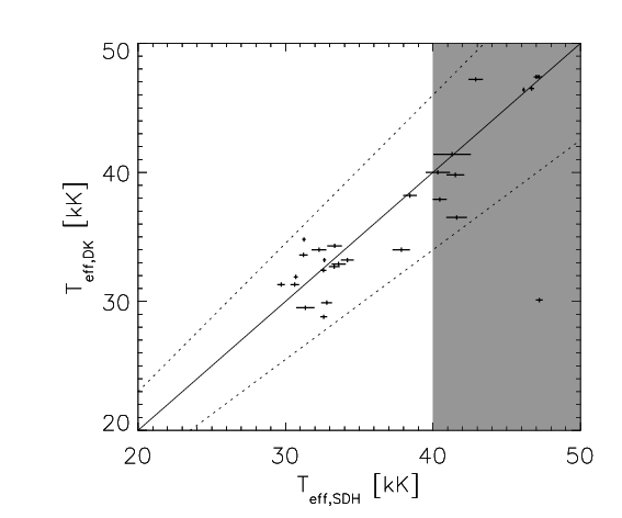
Our best fit models are shown in Figure 2 and the photospheric values are presented in Table 1. The comparison of our NLTE model fits to the temperature values obtained with LTE Koester models is shown in Figure 1. Our derived temperatures are in better agreement with the fitting method of Koester. This is not very surprising since the procedures are very similar. The Eisenstein autofit method fits photometric data additionally to the spectroscopy.

The left panel plot in Figure 1 shows that our fitting method, especially in the high temperature regime, produces higher $T_{\rm eff}$ values than the Eisenstein method. However, all but two fits – one of which is for an object with a significant amount of hydrogen and therefore cannot be reliably fit with our He-rich models– are within the 15% deviation range. The Koester fits are in even better agreement with our model fitting. Direct comparison of our non-LTE to the LTE Koester models show some obvious deviations in the continuum flux which increase towards lower temperatures. Currently, we do not have an explanation for these discrepancies.

Overall, we can confirm the results of Eisenstein et al. (2006). Especially the nice agreement of our fits to those of Koester at effective temperatures $>45~{\rm K}$ suggests that LTE is a valid assumption for the analysis of DB-gap white dwarfs.

Refer to caption — Figure 1: Comparison of LTE effective temperatures from the Eisenstein (left panel) and Koester (right panel) fits to our NLTE fits for all analysed WDs. The Eisenstein fits show systematically lower temperatures than the Koester fits. The latter ones agree better with our fitting results. The shaded area is the temperature range where we expect deviations from LTE, i. e. differences in fitted temperatures. The dotted lines are 15% deviations from equality (solid lines).

Table 1: Best-fit model values for the analyzed SDSS spectra. SDSS J153852.35-012133.8 clearly shows hydrogen Balmer lines and cannot be fit with our model grid. The real effective temperature is lower than the value given in this table. All errors are

1

\sigma

statistical errors.

Name	$T_{\rm eff}~{\rm[K]}$		$\log{g}$ (cgs)		$X({\rm He})$	$\chi^{2}$
SDSS J001529.75+010521.4	40325 $\pm$	821	7.88 $\pm$	0.07	99.9	1.1601
SDSS J040854.60 $-$ 043354.7	41607 $\pm$	697	7.76 $\pm$	0.04	99.0	1.2157
SDSS J074538.17+312205.4	42890 $\pm$	483	7.72 $\pm$	0.06	99.9	1.2050
SDSS J081115.09+270621.8	47007 $\pm$	168	7.91 $\pm$	0.03	99.0	1.1289
SDSS J081546.08+244603.3	46692 $\pm$	157	7.92 $\pm$	0.04	99.0	1.1678
SDSS J084823.53+033216.7	33327 $\pm$	495	7.75 $\pm$	0.07	99.0	1.1150
SDSS J084916.18+013721.3	31347 $\pm$	618	8.03 $\pm$	0.04	99.9	1.1431
SDSS J090232.18+071930.0	32787 $\pm$	360	7.96 $\pm$	0.03	99.9	1.1815
SDSS J090456.13+525029.9	38435 $\pm$	461	7.60 $\pm$	0.01	99.0	1.2014
SDSS J092544.41+414803.2	41517 $\pm$	596	7.83 $\pm$	0.10	99.9	1.1468
SDSS J093041.80+011508.4	37850 $\pm$	585	7.60 $\pm$	0.01	99.9	1.1464
SDSS J093759.52+091653.3	29705 $\pm$	247	8.23 $\pm$	0.01	99.9	1.2879
SDSS J095256.69+015407.7	31257 $\pm$	112	8.23 $\pm$	0.01	99.9	1.2535
SDSS J113609.59+484318.9	46152 $\pm$	90	8.17 $\pm$	0.01	99.9	1.4391
SDSS J123750.47+085526.0	32270 $\pm$	495	8.24 $\pm$	0.03	99.9	1.1364
SDSS J134524.92 $-$ 023714.2	41292 $\pm$	1260	7.96 $\pm$	0.03	99.9	1.2249
SDSS J140159.09+022126.7	40460 $\pm$	461	7.99 $\pm$	0.03	99.9	1.1346
SDSS J141258.17+045602.2	30695 $\pm$	135	8.19 $\pm$	0.01	99.9	1.3531
SDSS J141349.46+571716.4	30627 $\pm$	292	8.17 $\pm$	0.02	99.9	1.1883
SDSS J143227.25+363215.2	33305 $\pm$	360	7.91 $\pm$	0.04	99.9	1.1576
SDSS J153852.35 $-$ 012133.8	47210 $\pm$	225	7.60 $\pm$	0.01	99.0	1.1996
SDSS J154201.50+502532.1	32630 $\pm$	101	7.96 $\pm$	0.01	99.9	1.4335
SDSS J164703.44+245129.1	34182 $\pm$	427	7.60 $\pm$	0.01	99.9	1.1683
SDSS J211149.60 $-$ 053938.4	47165 $\pm$	202	7.74 $\pm$	0.05	99.0	1.1400
SDSS J212403.12+114230.2	32562 $\pm$	202	7.99 $\pm$	0.02	99.9	1.2352
SDSS J215514.44 $-$ 075833.8	32585 $\pm$	225	8.05 $\pm$	0.02	99.9	1.1418
SDSS J222833.82+141037.0	31212 $\pm$	270	8.32 $\pm$	0.03	99.9	1.1198
SDSS J234709.29+001858.0	33597 $\pm$	472	7.96 $\pm$	0.05	99.9	1.2369

References

Dreizler, S. & Werner, K. 1996 A&A 314 217
Eisenstein, D. J., Liebert, J., Koester, D., et al. 2006 AJ 132 676
Hügelmeyer, S. D., Dreizler, S., Homeier, D., et al. 2006 A&A 454 617
Liebert, J., Wesemael, F., Hansen, C. J., et al. 1986 ApJ 309 241
Wesemael, F., Green, R. F., & Liebert, J. 1985 ApJS 58 379