Low energy analysis of $\nu N\to\nu N\gamma$ in the Standard Model

Preprint: EFI Preprint 09-05

Richard J. Hill Email: richardhill@uchicago.edu Affiliation: Enrico Fermi Institute and Department of Physics
The University of Chicago, Chicago, Illinois, 60637, USA

August 24, 2026

Abstract

The production of single photons in low energy ( $\sim$ 1 GeV) neutrino scattering off nucleons is analyzed in the Standard Model. At very low energies, $E_{\nu}\ll{\rm GeV}$ , a simple description of the chiral lagrangian involving baryons and arbitrary $SU(2)_{L}\times U(1)_{Y}$ gauge fields is developed. Extrapolation of the process into the $\sim 1-2\,{\rm GeV}$ region is treated in a simple phenomenological model. Coherent enhancements in compound nuclei are studied. The relevance of single photon events as a background to experimental searches for $\nu_{\mu}\to\nu_{e}$ is discussed. In particular, single photons are a plausible explanation for excess events observed by the MiniBooNE experiment.

pacs

12.38.Qk, 12.39.Fe, 13.15.+g,

I Introduction

Recently, it was shown that a careful gauging of the low energy chiral lagrangian of QCD leads to new anomalous interactions, “pseudo Chern Simons” (pCS) interactions, between the $Z$ -boson, the photon and strongly coupled vector mesons, such as the spin- $1$ $\omega$ meson, taking the form $\propto\epsilon^{\mu\nu\rho\sigma}\omega_{\mu}Z_{\nu}F_{\rho\sigma}$ [1]. At low energies, this interaction implies anomalous processes involving neutrinos and $\gamma$ ’s in the presence of nuclear fields, e.g. contributing to $\nu N\to\nu N\gamma$ .

Previous simple estimates suggest that these effects may be at work in experimental configurations such as MiniBooNE [2]. They can lead to a peculiar enhancement in the appearance of “electrons” in a $\nu_{\mu}$ beam, where the hard $\gamma$ ’s are actually faking electron Cerenkov signatures [3]. This phenomenon may also play a role in astrophysical applications such as in neutron star cooling and supernova dynamics. The present paper widens the analysis of the phenomenology of such novel interactions, focusing on laboratory detection.

A rigorous discussion of photon production by the weak neutral current can be obtained at low neutrino energies using a chiral lagrangian description. Section II reviews the key aspects of the chiral lagrangian in the presence of baryons, and extends the usual formalism to describe general vector and axial-vector couplings of neutral electroweak fields. Terms induced by the pCS interactions appear at 3-derivative order, and are described by an essentially unique new operator appearing at this order. The effects of this interaction may be accessible in processes such as radiative neutrino scattering on baryons, or in certain parity violating observables¹¹ 1 For example, in analogy to the discussion in [3], the pCS interactions induce an anapole moment at finite baryon density. .

Section III investigates in more detail the processes of Compton-like scattering (with a weak vector or axial-vector current replacing one of the photons), $t$ -channel $\omega(780)$ resonance exchange, and $s$ -channel $\Delta(1232)$ resonance production. These processes serve to fix the normalization of the relevant interactions appearing in the chiral lagrangian, and provide a form-factor model to extrapolate the phenomenological predictions into the $E_{\nu}\sim 1\,{\rm GeV}$ energy range. An explicit computation of the competing contributions involving the axial-vector weak current reveals the significance of the operator induced by the above-mentioned pCS term: it is the unique interaction appearing through 3-derivative order in the chiral lagrangian that leads to a coherent coupling of one axial-vector gauge field and one vector gauge field to baryons. A significant contribution to the coefficient of this operator is also induced from the $\Delta$ resonance. Pertinent details of the $\Delta$ coupling to baryons and gauge fields are reviewed. The relevance of “off-shell” parameters for the $\Delta$ couplings to nucleons and vector currents is investigated, and simplifications in the formal large- $N_{c}$ limit are discussed.

Section IV presents cross section estimates for single-photon production in neutrino-nucleon scattering, i.e., $\nu(\overline{\nu})n\to\nu(\overline{\nu})n\gamma$ , $\nu(\overline{\nu})p\to\nu(\overline{\nu})p\gamma$ . Section V discusses several aspects of coherent scattering on compound nuclei, and derives scaling laws for the coherent cross sections in the limit of a large nucleus. Section VI concludes with a brief discussion on the relevance of single photon production as a background to experiments searching for $\nu_{\mu}\to\nu_{e}$ oscillation, and an outline for future work.

II Chiral lagrangian for nonrelativistic baryons and electroweak gauge fields

Consider physical processes involving a single nucleon interacting with electroweak fields at energies small compared to typical hadronic scales $\sim 1\,{\rm GeV}$ . The relevant dynamical fields include the pions, identified as Nambu-Goldstone bosons (NGBs) of spontaneously broken chiral symmetry; the nucleons; and the electroweak fields. To begin, let us concentrate on processes involving almost-stationary nucleons, so that a nonrelativistic expansion is appropriate. The task is to build the most general effective lagrangian from these fields, order by order in the small parameters $E/m_{N}\sim E/4\pi f_{\pi}\ll 1$ . The full nonrelativistic expansion is cumbersome [4], and for a tree-level analysis it is simpler to work in a manifestly Lorentz-invariant form of the Lagrangian. The basic formalism is common to previous analyses [5, 6, 7], which however neglect a systematic treatment of the $U(1)$ factors. Care will be taken to include the full $SU(2)_{L}\times SU(2)_{R}\times U(1)_{V}$ symmetry that encompasses the Standard Model gauge group.

II.1 Fields in the effective theory

Let us first make a few comments on the treatment of NGBs, nucleons and electroweak gauge fields in the effective theory. This will also serve to introduce notations and conventions. As usual, the pions are collected into the $SU(2)$ matrix field (considering for simplicity just $n_{f}=2$ light flavors),

U=\exp[(2i/f_{\pi})\pi^{a}T^{a}]\,,

(1)

with $T^{a}=\tau^{a}/2$ and $f_{\pi}\approx 93\,{\rm MeV}$ .

The nucleons $p$ and $n$ compose a field

N=\left(\begin{array}[]{c}p\\ n\end{array}\right)\,,

(2)

that transforms linearly under isospin. Extending linear $SU(2)_{V}$ isospin transformations to general $SU(2)_{L}\times SU(2)_{R}$ requires a nonlinear transformation law that reduces to the linear one when restricted to the unbroken $SU(2)_{V}$ subgroup [8]. This is achieved by introducing a field $\xi$ such that

\xi^{2}=U\,.

(3)

Consider an $SU(2)_{L}\times SU(2)_{R}\times U(1)_{V}$ transformation of the underlying quarks: $\psi_{L,R}\to e^{i\epsilon_{L,R}}\psi_{L,R}$ . Then $U$ is defined to transform as:

U\to e^{i\epsilon_{L}}Ue^{-i\epsilon_{R}}\,,

(4)

and we can further define a quantity $\epsilon^{\prime}$ by requiring the corresponding transformation law of $\xi$ :

\xi\to e^{i\epsilon_{L}}\xi e^{-i\epsilon^{\prime}}=e^{i\epsilon^{\prime}}\xi e^{-i\epsilon_{R}}\,.

(5)

Finally, we define $N$ to transform as

N\to\exp\left[i\left(\hat{\epsilon}^{\prime}+\frac{3}{2}{\rm Tr}(\epsilon^{\prime})\right)\right]N\,.

(6)

Here $\hat{M}\equiv M-\frac{1}{2}{\rm Tr}(M)$ denotes the traceless part of a general $2\times 2$ matrix $M$ . Note that the factor of $3$ in front of ${\rm Tr}(\epsilon^{\prime})$ reflects the underlying quark content of the nucleons.

Now consider the usual $SU(2)_{L}\times U(1)_{Y}$ gauge subgroup of the Standard Model. At the physical value of the electroweak coupling constant $g_{2}$ , and Higgs vacuum expectation value $v_{\rm weak}$ , the $W$ and $Z$ bosons are very heavy, $m_{W,Z}\sim g_{2}v_{\rm weak}$ , and are integrated out of the theory. In order to keep track of gauge-invariance constraints that survive at low-energy, first consider the limit $v_{\rm weak}\gg f_{\pi}$ fixed and $g_{2}$ small. In this case, $W$ and $Z$ still eat mostly the Higgs NGBs (not the pions) but have small mass. At the end of the analysis, $g_{2}$ can then be set to its physical value and the massive vector bosons integrated out to induce operators involving only light fields (such as leptons).

II.2 Covariant building blocks and effective lagrangian

Let $A_{L}^{\mu}$ and $A_{R}^{\mu}$ represent weakly coupled gauge fields (or external fields) acting on left- and right-handed quark fields, and let us define

	$\displaystyle\tilde{A}_{L}^{\mu}$	$\displaystyle\equiv\xi^{\dagger}(i\partial^{\mu}+A_{L}^{\mu})\xi\,,$
	$\displaystyle\tilde{A}_{R}^{\mu}$	$\displaystyle\equiv\xi(i\partial^{\mu}+A_{R}^{\mu})\xi^{\dagger}\,.$		(7)

These objects have the transformation laws,

	$\displaystyle\tilde{A}_{L}^{\mu}$	$\displaystyle\to e^{i\epsilon^{\prime}}(\tilde{A}_{L}^{\mu}+i\partial^{\mu})e^{-i\epsilon^{\prime}}\,,$
	$\displaystyle\tilde{A}_{R}^{\mu}$	$\displaystyle\to e^{i\epsilon^{\prime}}(\tilde{A}_{R}^{\mu}+i\partial^{\mu})e^{-i\epsilon^{\prime}}\,.$		(8)

Under parity, the fields transform as

\xi\leftrightarrow\xi^{\dagger}\,,\quad A_{L}\leftrightarrow A_{R}\,,

(9)

so that

\tilde{A}_{L}\leftrightarrow\tilde{A}_{R}\,.

(10)

Fields with definite parity are the linear combinations

	$\displaystyle\tilde{V}$	$\displaystyle\equiv\frac{1}{2}\left(\tilde{A}_{L}+\tilde{A}_{R}\right)\,,$
	$\displaystyle\tilde{A}$	$\displaystyle\equiv\frac{1}{2}\left(\tilde{A}_{L}-\tilde{A}_{R}\right)\,,$		(11)

transforming under parity as vector and axial-vector, respectively. Under a gauge transformation we have

	$\displaystyle\tilde{V}_{\mu}$	$\displaystyle\to e^{i\epsilon^{\prime}}(\tilde{V}_{\mu}+i\partial_{\mu})e^{-i\epsilon^{\prime}}\,,$
	$\displaystyle\tilde{A}_{\mu}$	$\displaystyle\to e^{i\epsilon^{\prime}}\tilde{A}_{\mu}e^{-i\epsilon^{\prime}}\,.$		(12)

Eq. (6), shows that in order to build invariant operators involving the nucleon field, the trace component of the vector field should appear as:

\displaystyle\tilde{V}^{\prime}_{\mu}\equiv\hat{\tilde{V}}_{\mu}+\frac{3}{2}{\rm Tr}(\tilde{V}_{\mu})

\displaystyle\to\exp\left[i\left(\hat{\epsilon}^{\prime}+\frac{3}{2}{\rm Tr}(\epsilon^{\prime})\right)\right]\big(\tilde{V}^{\prime}_{\mu}+i\partial_{\mu}\big)\,\exp\left[-i\left(\hat{\epsilon}^{\prime}+\frac{3}{2}{\rm Tr}(\epsilon^{\prime})\right)\right]\,.

(13)

Thus $\tilde{A}$ is a covariantly transforming axial-vector field, and $\tilde{V}^{\prime}$ is a vector field that can be used to form the covariant derivative acting on nucleon fields,

i\tilde{D}_{\mu}=i\partial_{\mu}+\tilde{V}^{\prime}_{\mu}\,.

(14)

Explicitly, the leading expansions for vector and axial-vector fields are

	$\displaystyle\tilde{V}^{\prime}_{\mu}$	$\displaystyle={g_{2}\over 4}\left(\begin{array}[]{cc}{1\over c_{W}}(1-4s_{W}^{2})Z_{\mu}&\sqrt{2}W^{+}_{\mu}\\ \sqrt{2}W^{-}_{\mu}&-{1\over c_{W}}Z_{\mu}\end{array}\right)+e\left(\begin{array}[]{cc}A^{\rm e.m.}_{\mu}&0\\ 0&0\end{array}\right)+\dots\,,$
	$\displaystyle\tilde{A}_{\mu}$	$\displaystyle={g_{2}\over 4}\left(\begin{array}[]{cc}{1\over c_{W}}Z_{\mu}&\sqrt{2}W^{+}_{\mu}\\ \sqrt{2}W^{-}_{\mu}&-{1\over c_{W}}Z_{\mu}\end{array}\right)-{1\over 2f_{\pi}}\left(\begin{array}[]{cc}\partial_{\mu}\pi^{0}&\sqrt{2}\partial_{\mu}\pi^{+}\\ \sqrt{2}\partial_{\mu}\pi^{-}&-\partial_{\mu}\pi^{0}\end{array}\right)+\dots\,,$

where dots denotes terms with two or more pions. The notation $s_{W}=\sin\theta_{W}$ , $c_{W}=\cos\theta_{W}$ is used throughout, where $s_{W}^{2}=0.231$ .

It is now straightforward to write down the Lagrangian working order by order in derivatives. Consider the expansion through three-derivative order, where the interesting effects of pCS terms make their appearance. In the one-baryon sector,

{\cal L}=m_{N}{\cal L}^{(0)}+{\cal L}^{(1)}+{1\over m_{N}}{\cal L}^{(2)}+{1\over m_{N}^{2}}{\cal L}^{(3)}+\dots\,,

(23)

where for convenience the mass scale in the expansion is defined as the nucleon mass, $m_{N}\approx 940\,{\rm MeV}$ . For notational simplicity, the tildes on fields are dropped in the remainder of this section. Using hermiticity and enforcing invariance under parity and time-reversal, and making use of the leading-order equations of motion

	$\displaystyle(iD\!\!\!/\!\,\,-m_{N})N$	$\displaystyle\sim 0\,,$
	$\displaystyle[D_{\mu},{A}^{\mu}]$	$\displaystyle\sim 0\,,$		(24)

the result is:

$\displaystyle{\cal L}^{(0)}$	$\displaystyle=-c^{(0)}\overline{N}N\,,$
$\displaystyle{\cal L}^{(1)}$	$\displaystyle=\overline{N}\big[c^{(1)}_{1}iD\!\!\!/\!\,\,-c^{(1)}_{2}A\!\!\!/\!\,\,\gamma_{5}\big]N\,,$
$\displaystyle{\cal L}^{(2)}$	$\displaystyle=\overline{N}\big[-c^{(2)}_{1}\frac{i}{2}\sigma^{\mu\nu}{\rm Tr}([iD_{\mu}\,,iD_{\nu}])-c^{(2)}_{2}\frac{i}{2}\sigma^{\mu\nu}\tau^{a}{\rm Tr}(\tau^{a}[iD_{\mu}\,,iD_{\nu}])+\dots\big]N\,,$
$\displaystyle{\cal L}^{(3)}$	$\displaystyle=\overline{N}\big[c^{(3)}_{1}\gamma^{\nu}[iD_{\mu},{\rm Tr}([iD^{\mu},iD_{\nu}])]+c^{(3)}_{2}\gamma^{\nu}[iD_{\mu},\tau^{a}{\rm Tr}\big(\tau^{a}[iD^{\mu},iD_{\nu}]\big)]$
	$\displaystyle\qquad+c^{(3)}_{3}\gamma^{\nu}\gamma_{5}[iD_{\mu},[iD^{\mu},A_{\nu}]]$
	$\displaystyle\qquad+c^{(3)}_{4}i\epsilon^{\mu\nu\rho\sigma}\gamma_{\sigma}{\rm Tr}\big(\{A_{\mu},[iD_{\nu},iD_{\rho}]\}\big)+c^{(3)}_{5}i\epsilon^{\mu\nu\rho\sigma}\gamma_{\sigma}\tau^{a}{\rm Tr}\big(\tau^{a}\{A_{\mu},[iD_{\nu},iD_{\rho}]\}\big)$
	$\displaystyle\qquad+c^{(3)}_{6}\gamma^{\nu}\gamma_{5}[[iD_{\mu}\,,iD_{\nu}]\,,A^{\mu}]+c^{(3)}_{7}{1\over 4m_{N}^{2}}\gamma^{\nu}\gamma_{5}\big\{[[iD_{\mu}\,,iD_{\nu}]\,,A_{\rho}],\{iD^{\mu}\,,iD^{\rho}\}\big\}+\dots\big]N\,.$	(25)

The dots in ${\cal L}^{(2)}$ and ${\cal L}^{(3)}$ denote terms containing more than one $A$ field. The simplification ${\rm Tr}(A)=0$ has been made, which is sufficient for Standard Model applications. When restricted to isovector gauge couplings, these expressions are equivalent to previous results at second [5] and third [9] order. The treatment of $U(1)$ factors encoded by (6) and (13) allows also the isoscalar components of both the photon and $Z$ boson to be incorporated systematically²² 2 The $U(1)_{V}$ factor has either been ignored [5] or added by hand [7] in previous discussions where either only pions, or only pions and photons were relevant to the discussion. . In (25), field redefinitions have been used to arrange operators in a manner that allows a straightforward interpretation in terms of a vector meson dominance model. Note that in expanding in derivatives, care must be taken to notice that the time component counts as order one,

i\partial_{0}N\sim{\cal O}(m_{N})N\,,

(26)

and hence in a relativistic and gauge-invariant description, covariant derivatives $D_{\mu}$ acting on the nucleon field cannot be viewed as power suppressed. Within the approximations of interest (three derivative order, and no more than one axial-vector field), the final term in (25) is the only new operator induced by this subtlety [9].

Despite appearances, the expansion (25) is remarkably simple when applied to the problem at hand. The leading coefficients define the mass and field normalization, $c^{(0)}=c^{(1)}_{1}=1$ . The remaining first and second-order coefficients are related at tree level to well-known low-energy observables. Coefficient $c^{(1)}_{2}$ is the axial-vector coupling to nucleons: $c^{(1)}_{2}\equiv g_{A}\approx 1.26$ . Coefficients $c^{(2)}_{1,2}$ represent the isoscalar and isovector anomalous magnetic moments (in units $1/2m_{N}$ ), which at tree level would be: $c^{(2)}_{1}\approx\frac{1}{4}(a_{p}+a_{n})$ , $c^{(2)}_{2}\approx\frac{1}{4}(a_{p}-a_{n})$ , where $a_{p}=1.79$ and $a_{n}=-1.91$ . For the third-order constants, $c^{(3)}_{1}$ and $c^{(3)}_{2}$ correspond to form-factor corrections to the leading vector couplings; in a vector dominance approximation, $c^{(3)}_{1}\approx\frac{1}{2}{m_{N}^{2}/m_{\omega}^{2}}$ , $c^{(3)}_{2}\approx\frac{1}{2}{m_{N}^{2}/m_{\rho}^{2}}$ , and similarly for axial-vector coupling, $c^{(3)}_{3}\approx-g_{A}{m_{N}^{2}/m_{a_{1}}^{2}}$ .

We are left finally with $c^{(3)}_{4,5,6,7}$ . The coefficients $c^{(3)}_{6}$ and $c^{(3)}_{7}$ will not be relevant, since the corresponding operators vanish for neutral gauge fields such as the $Z^{0}$ and the photon. The coefficients $c^{(3)}_{4,5}$ contain the low-energy manifestation of the $\omega ZdA$ and $\rho ZdA$ vertices studied in Ref [1, 3], after integrating out $\omega$ and $\rho$ :

	$\displaystyle c^{(3)}_{4}(\omega)$	$\displaystyle\sim{9\over 32\pi^{2}}{g^{\prime 2}m_{N}^{2}\over m_{\omega}^{2}}\sim 1.5,$
	$\displaystyle c^{(3)}_{5}(\rho)$	$\displaystyle\sim{1\over 32\pi^{2}}{g^{2}m_{N}^{2}\over m_{\rho}^{2}}\sim 0.2\,.$		(27)

The conventions $\epsilon^{0123}=-1$ , $g^{\mu\nu}={\rm diag}(1,-1,-1,-1)$ are used throughout. The sign of $c_{4}^{(3)}(\omega)$ is fixed by noticing that the baryon current has divergence $\partial_{\mu}J^{\mu}=-(eg_{2}/8\pi^{2}c_{W})\epsilon^{\mu\nu\rho\sigma}\partial_{\mu}A^{\rm e.m.}_{\nu}\partial_{\rho}Z_{\sigma}+\dots$ , and enforcing that $\omega$ couples equally to all parts of the baryon current³³ 3 An errant minus sign appears in Eq.(76) of Ref. [1]. This is a transcription error from the (correct) Eq.(74) in the same reference. . We will see below that $c^{(3)}_{4}$ also receives significant contributions from $\Delta(1232)$ .

This discussion allows us to make more precise the significance of the pCS terms on low-energy physics: the operators that the pCS terms match onto are the only essentially new terms (i.e., besides terms representing form factor corrections to leading operators) in the baryon chiral lagrangian coupled to neutral vector and axial-vector fields through three derivative order. Such operators have the special property that they can act coherently on adjacent nucleons, yet involve axial-vector gauge fields.

II.3 Nonrelativistic expansion

In the relativistic formalism, there is not an explicit scale separation, for two reasons. First, the relativistic nucleon spinor contains suppressed terms

{u_{s}(k)\over\sqrt{2m_{N}}}\sim\left(\begin{array}[]{c}\chi_{s}\\ 0\end{array}\right)+{\bm{\sigma}\cdot\bm{k}\over 2m_{N}}\left(\begin{array}[]{c}0\\ \chi_{s}\end{array}\right)+\dots\,.

(28)

Second, there is an intermediate scale $Q^{2}\sim|\bm{p}|m_{N}$ that arises in diagrams such as Fig. 1:

{1\over(p+k)^{2}-m_{N}^{2}}={1\over 2p\cdot k+p^{2}}\sim{1\over 2|\bm{p}|m_{N}}\,.

(29)

For the present tree-level analysis, it is not technically necessary to make the scale separation

|\bm{p}|^{2}\ll|\bm{p}|m_{N}\ll m_{N}^{2}

(30)

explicit. However, since it is instructive to see how the various contributions to $\nu N\to\nu N\gamma$ arise in such a formalism, an outline is presented here.

II.3.1 Nonrelativistic fields and effective lagrangian

For nonrelativistic nucleons, the antiparticle components of the nucleon field are integrated out, and we deal with two-component (Pauli) spinor fields $\chi_{p}$ , $\chi_{n}$ , in place of four-component (Dirac) spinor fields. This expansion does not affect the chiral transformation properties, and the nonrelativistic isodoublet nucleon field transforms as before:

\hat{N}=\left(\begin{array}[]{c}\chi_{p}\\ \chi_{n}\end{array}\right)\to e^{i\epsilon^{\prime}}\hat{N}\,,

(31)

where hats are here used to denote nonrelativistic fields. (For a proper treatment of the $U(1)$ factors, the modification (6) is understood.)

Invariant combinations can be formed from the operators:

D_{0}\,,A_{0}\,,D_{i}\,,A_{i}\,,

(32)

sandwiched between $\hat{N}^{\dagger}(\dots)\hat{N}$ . Let us denote the expansion as

\hat{\cal L}=m_{N}\hat{\cal L}^{(0)}+\hat{\cal L}^{(1)}+{1\over m_{N}}\hat{\cal L}^{(2)}+{1\over m_{N}^{2}}\hat{\cal L}^{(3)}+\dots\,.

(33)

Lorentz symmetry is broken by the nonrelativistic limit, but parity, time-reversal and rotation invariance of the strong interactions is preserved. In particular, the fields $D_{i}$ and $A_{0}$ are odd under parity, and so must appear an even number of times.

At zeroth order,

\hat{\cal L}^{(0)}=\hat{c}^{(0)}\hat{N}^{\dagger}\hat{N}\,.

(34)

By an appropriate field redefinition ( $\hat{N}\to e^{-im_{N}t}\hat{N}$ ), this term can be removed, $\hat{c}^{(0)}\equiv 0$ . At first order,

\hat{\cal L}^{(1)}=\hat{N}^{\dagger}(\hat{c}^{(1)}_{1}iD_{0}+\hat{c}^{(1)}_{2}\bm{\sigma}\cdot\bm{A})\hat{N}\,.

(35)

The normalization of the field $\hat{N}$ can be chosen such that $\hat{c}^{(1)}_{1}\equiv 1$ and then $\hat{c}^{(1)}_{2}$ determines the tree-level axial-vector coupling. At second order,

\displaystyle\hat{\cal L}^{(2)}

\displaystyle=\hat{N}^{\dagger}\bigg(\!\!-\frac{1}{2}\hat{c}^{(2)}_{1}\bm{D}^{2}+\hat{c}^{(2)}_{2}\epsilon^{ijk}\sigma^{i}{\rm Tr}(D_{j}D_{k})+\hat{c}^{(2)}_{3}\epsilon^{ijk}\sigma^{i}\tau^{a}{\rm Tr}(\tau^{a}D_{j}D_{k})+i\hat{c}^{(2)}_{4}\{\bm{\sigma}\cdot\bm{D},A_{0}\}\!\!\bigg)\hat{N}\,,

(36)

where the leading order equation of motion,

iD_{0}\hat{N}\sim 0\,,

(37)

is used to eliminate additional terms containing $D_{0}$ . The first term in $\hat{\cal L}^{(2)}$ defines the nucleon mass, ${\hat{c}^{(2)}_{1}}\equiv 1$ . For the remaining terms, ${\hat{c}^{(2)}_{2}}$ and ${\hat{c}^{(2)}_{3}}$ give the isoscalar and isovector magnetic moments, and ${\hat{c}^{(2)}_{4}}$ is a relativistic correction to the axial-vector coupling.

At third order, the number of terms continues to proliferate. Many of these are, at tree level, simply relativistic corrections to the leading order terms that are summed automatically in the relativistic formalism. For simplicity in the present discussion, let us concentrate on those operators that do not involve the nucleon spin, i.e., operators that can give rise to coherent interactions on adjacent nucleons. This case is particularly simple, and there is a unique operator up to isospin combinations,

\displaystyle\hat{\cal L}^{(3)}

\displaystyle=\hat{N}^{\dagger}\bigg(\hat{c}^{(3)}_{1}\epsilon^{ijk}{\rm Tr}(A_{i}D_{j}D_{k})+\hat{c}^{(3)}_{2}\epsilon^{ijk}\tau^{a}{\rm Tr}(\tau^{a}A_{i}D_{j}D_{k})+\dots\bigg)\hat{N}\,.

(38)

These operators are mapped onto by the $\rho$ and $\omega$ exchange discussed earlier, The expansions (35),(36),(38) show explicitly that the operators parameterized by $\hat{c}^{(3)}_{1,2}$ in (38), and hence $c^{(3)}_{4,5}$ in (25), are the only direct interactions with a coherent coupling of one vector and one axial-vector field to the nucleon through three-derivative order. Eqs.(51) and Appendix A below will verify that iterations of ${\cal L}^{(1)}$ and ${\cal L}^{(2)}$ do not give rise to further coherent interactions. This justifies the statement made at the end of the previous section regarding the unique property of the operator induced by the pCS terms, i.e., coherent coupling of vector and axial-vector fields to the nucleon.

II.3.2 Low energy: integrating out the intermediate mass scale

Since the nucleon kinetic energy is

E_{N}-m_{N}\sim\bm{k}^{2}/2m_{N}\ll|\bm{k}|\,,

(39)

any exchange of energy of order $|\bm{k}|$ takes the nucleon far offshell. At very low energies we should integrate out such modes, making use of the scale separation $m_{N}^{2}\gg m_{N}|\bm{k}|\gg|\bm{k}|^{2}$ . The scale $m_{N}^{2}$ was integrated out in the previous step, summarized by (33) (the same is accomplished, though not explicitly, by (23) in the relativistic formulation).

Contributions to the Compton-like scattering process depicted in Fig. 1 begin at ${\cal O}(1/m_{N})$ . Leading contributions involve a single insertion of $\hat{\cal L}^{(2)}$ , while subleading contributions arise from either two insertions of $\hat{\cal L}^{(2)}$ , or a single insertion of $\hat{\cal L}^{(3)}$ . Such combinations of $\hat{\cal L}^{(1)}$ and $\hat{\cal L}^{(2)}$ are described at very low energy by local contact interactions corresponding to the amplitudes derived below in (51) and (114). In addition, there is the direct contribution from $\hat{\cal L}^{(3)}$ , corresponding to (59) below. The competing energy scales for these different contributions are ${1/(m_{N}E)}$ for the Compton-like process, versus $1/m_{\rho}^{2}\sim 1/m_{\omega}^{2}$ for the meson exchange.

The nonrelativistic expansion provides an explicit scale separation that is insightful but not essential at tree level. Rather than pursue a more formal description of this low-energy effective theory, the relevant amplitudes are calculated in the following sections directly from the relativistic formulation (25).

III Low-energy constants and large-energy extrapolation

In order to proceed phenomenologically, the normalizations (Wilson coefficients or low-energy constants) for the relevant interactions of the lagrangian (25) must be fixed, and a reasonable model (form factors) must be specified for extrapolating into the ${\rm GeV}$ energy range where the chiral lagrangian is breaking down.

It should be emphasized that in extrapolating to larger energy, we are leaving the firm theoretical footing of the chiral lagrangian. The simplest form factors based on vector dominance are still predictions obtained at tree level from a well-defined effective lagrangian (including vector mesons), albeit with significant corrections from neglected loop effects. Introducing phenomenological form factors takes us further from a simple effective lagrangian approach, but crudely accounts for effects of higher resonances, and provides a connection to higher energy via perturbative scaling laws that must be satisfied when momentum invariants are large. Formal justification for this approach, in particular approximating amplitudes by tree level exchange of physical mesons, can be found in a large $N_{c}$ (number of colors) limit [10]. Given the relatively modest extrapolations involved (e.g. up to $E_{\nu}\sim 1.5\,{\rm GeV}$ ), and the absence of a more controlled expansion scheme in this energy regime, the remainder of the paper proceeds without further apology.

The rest of this section investigates the mechanisms of generalized Compton scattering; $t$ -channel $\omega$ (and $\rho$ , $\pi$ ) exchange; and $s$ -channel $\Delta$ production. These mechanisms include the direct couplings of the electroweak gauge fields to nucleons, and incorporate effects of the dominant hadronic resonances in each channel.

III.1 Compton scattering

Refer to caption — Figure 1: Generalized compton scattering.

Let us begin by examining the contributions to $\nu N\to\nu N\gamma$ mediated by an intermediate nucleon as depicted in Fig. 1. These contributions will be referred to as “Compton-like” scattering where one of the photons is replaced by an (offshell) $Z$ boson. As discussed above, form factors for onshell nucleons are employed at the vertices to account for resonant structure in the appropriate channel.

III.1.1 Form factors

The onshell matrix element of the weak neutral current and electromagnetic current take the form

	$\displaystyle\langle N(k^{\prime})\|J_{\rm NC}^{\mu}\|N(k)\rangle$	$\displaystyle={g_{2}\over 2c_{W}}\overline{u}(k^{\prime})\Gamma_{\rm NC}^{\mu}(k^{\prime}-k)u(k)\,,$
	$\displaystyle\langle N(k^{\prime})\|J_{\rm em}^{\mu}\|N(k)\rangle$	$\displaystyle=e\,\overline{u}(k^{\prime})\Gamma_{\rm em}^{\mu}(k^{\prime}-k)u(k)\,.$		(40)

For the weak neutral current

\displaystyle\Gamma_{\rm NC}^{\mu}(q)

\displaystyle=\gamma^{\mu}[F^{1\,,\rm weak}_{V}(q^{2})-F_{A}(q^{2})\gamma_{5}]+{i\over 2m_{N}}\sigma^{\mu\nu}q_{\nu}F_{V}^{2\,,\rm weak}(q^{2})+{1\over m_{N}}F_{P}(q^{2})q^{\mu}\gamma_{5}\,,

(41)

and similarly, for the electromagnetic current:

\displaystyle\Gamma_{\rm em}^{\mu}(q^{2})

\displaystyle=\gamma^{\mu}F^{1\,,\rm em}_{V}(q^{2})+{i\over 2m_{N}}\sigma^{\mu\nu}q_{\nu}F_{V}^{2\,,\rm em}(q^{2})\,.

(42)

Enforcing time-reversal invariance ensures that $F_{V}^{1,2}(0)$ , $F_{A}(0)$ and $F_{P}(0)$ are real as expected from the effective lagrangian (25). Note that $F_{P}$ in (41) is induced by pion exchange, and is not represented by a new operator in the theory [11]. The contribution from $F_{P}$ vanishes when the current couples to massless leptons (e.g., in the approximation of massless neutrinos), and will not be relevant here.

Standard parameterizations in terms of the electric and magnetic form factors are used: [12]

	$\displaystyle G_{E}$	$\displaystyle\equiv F^{1}+{q^{2}\over 4m_{N}^{2}}F^{2}\,,$
	$\displaystyle G_{M}$	$\displaystyle\equiv F^{1}+F^{2}\,,$		(43)

with

G_{E\,\rm proton}\approx{G_{M\,\rm proton}\over 1+a_{p}}\approx{G_{M\,\rm neutron}\over a_{n}}\approx{1\over(1-q^{2}/0.71\,{\rm GeV}^{2})^{2}}\equiv F_{D}(q^{2})\,.

(44)

In terms of the common overall dipole factor, the electromagnetic form factors of the proton are:

	$\displaystyle F^{1\,,\rm em}_{V\,\rm proton}/F_{D}$	$\displaystyle=1-{q^{2}/4m_{N}^{2}\over 1-q^{2}/4m_{N}^{2}}a_{p}\,,$
	$\displaystyle F^{2\,,\rm em}_{V\,\rm proton}/F_{D}$	$\displaystyle={a_{p}\over 1-q^{2}/4m_{N}^{2}}\,,$		(45)

and for the neutron:

	$\displaystyle F^{1\,,\rm em}_{V\,\rm neutron}/F_{D}$	$\displaystyle=-{q^{2}/4m_{N}^{2}\over 1-q^{2}/4m_{N}^{2}}a_{n}\,,$
	$\displaystyle F^{2\,,\rm em}_{V\,\rm neutron}/F_{D}$	$\displaystyle={a_{n}\over 1-q^{2}/4m_{N}^{2}}\,.$		(46)

Similarly, for the weak current, for the proton:

	$\displaystyle F^{1\,,\rm weak}_{V\,\rm proton}/F_{D}$	$\displaystyle=\frac{1}{2}-2s_{W}^{2}-{q^{2}/4m_{N}^{2}\over 1-q^{2}/4m_{N}^{2}}\left[\left(\frac{1}{2}-2s_{W}^{2}\right)a_{p}-\frac{1}{2}a_{n}\right]\,,$
	$\displaystyle F^{2\,,\rm weak}_{V\,\rm proton}/F_{D}$	$\displaystyle={1\over 1-q^{2}/4m_{N}^{2}}\left[\left(\frac{1}{2}-2s_{W}^{2}\right)a_{p}-\frac{1}{2}a_{n}\right]\,,$		(47)

and for the neutron:

	$\displaystyle F^{1\,,\rm weak}_{V\,\rm neutron}/F_{D}$	$\displaystyle=-\frac{1}{2}-{q^{2}/4m_{N}^{2}\over 1-q^{2}/4m_{N}^{2}}\left[\left(\frac{1}{2}-2s_{W}^{2}\right)a_{n}-\frac{1}{2}a_{p}\right]\,,$
	$\displaystyle F^{2\,,\rm weak}_{V\,\rm neutron}/F_{D}$	$\displaystyle={1\over 1-q^{2}/4m_{N}^{2}}\left[\left(\frac{1}{2}-2s_{W}^{2}\right)a_{n}-\frac{1}{2}a_{p}\right]\,.$		(48)

At $q^{2}=0$ the weak form factors reduce to $F^{1\,,\rm weak}_{V\,\rm proton}(0)\equiv C_{V\,\rm proton}=\frac{1}{2}-2s_{W}^{2}$ , $F^{1\,,\rm weak}_{V\,\rm neutron}(0)\equiv C_{V\,\rm neutron}=-\frac{1}{2}$ . Finally, a standard prescription is used for the axial-vector form factor:

F_{A}(q^{2})={F_{A}(0)\over(1-q^{2}/m_{A}^{2})^{2}}\,,

(49)

with axial mass parameter $m_{A}\approx 1.2\,{\rm GeV}$ [13]. For the normalization of the axial-vector coupling, strange quark effects are ignored and the interaction is pure isovector:

F_{A\,\rm proton}(0)\equiv C_{A\,\rm proton}=-F_{A,\rm neutron}(0)\equiv-C_{A\,\rm neutron}=1.26/2\,.

(50)

The dipole form factors (44) and (49) reproduce the correct perturbative scaling behavior at $q^{2}\to\infty$ [14].

III.1.2 Leading order cross section

Consider the low energy limit, or equivalently the limit $m_{N}\to\infty$ . The amplitude for $Z(p)+N(k)\to\gamma(q)+N(k^{\prime})$ from the diagrams in Fig. 1 is:

$\displaystyle i{\cal M}=-{ieg_{2}\over c_{W}}\,\chi^{\dagger}\bigg\{$	$\displaystyle\epsilon^{(\gamma)*}_{0}\epsilon^{(Z)}_{0}\bigg[F^{1}C_{V}\hat{\bm{p}}\cdot\hat{\bm{q}}-F^{1}C_{A}\hat{\bm{q}}\cdot\vec{\bm{\sigma}}\bigg]$
$\displaystyle+$	$\displaystyle\epsilon^{(\gamma)*}_{i}\epsilon^{(Z)}_{0}\bigg[F^{1}C_{V}\hat{p}^{i}-F^{1}C_{A}\sigma^{i}\bigg]$
$\displaystyle+$	$\displaystyle\epsilon^{(\gamma)*}_{0}\epsilon^{(Z)}_{j}\bigg[F^{1}C_{V}\hat{q}^{j}-F^{1}C_{A}\hat{\bm{p}}\cdot\hat{\bm{q}}\sigma^{j}\bigg]$
$\displaystyle+$	$\displaystyle\epsilon^{(\gamma)*}_{i}\epsilon^{(Z)}_{j}\bigg[F^{1}C_{V}\delta^{ij}-F^{1}C_{A}\left(\hat{p}^{i}\sigma^{j}+\hat{q}^{j}\sigma^{i}-\delta^{ij}\hat{\bm{q}}\cdot{\bm{\sigma}}\right)$
	$\displaystyle\qquad\qquad-F^{2}C_{A}(\hat{q}^{j}\sigma^{i}-\delta^{ij}\hat{\bm{q}}\cdot{\bm{\sigma}})\bigg]\bigg\}\chi\,.$	(51)

When, as in reality, the $Z$ is virtual and connected to the neutrino line, the amplitude is given by the replacements

	$\displaystyle{g_{2}\over 2c_{W}}\epsilon^{(Z)}_{\mu}$	$\displaystyle\to-{G_{F}\over\sqrt{2}}\overline{\nu}(p^{\prime})\gamma_{\mu}(1-\gamma_{5})\nu(p)\,,$
	$\displaystyle\hat{p}^{i}$	$\displaystyle\to{1\over E_{\gamma}}(p^{i}-p^{\prime i})\,,$		(52)

where the reaction is $\nu(p)N(k)\to\nu(p^{\prime})N(k^{\prime})\gamma(q)$ . Note that terms with $C_{A}$ involve spin-flip matrix elements, and hence the amplitudes for scattering on adjacent nuclei cannot add coherently. Appendix A verifies this property also at the next derivative order. These computations complete the discussion after (38): the operators induced by the pCS terms give the only contributions through three derivative order that involve the axial component of the $Z$ boson, and that can be coherent on adjacent nucleons.

Taking the $m_{N}\to\infty$ limit of the final state phase space, the cross section for $\nu N\to\nu N\gamma$ arising from generalized Compton scattering becomes

$\displaystyle{d\sigma({\rm Compton})\over dedx}$	$\displaystyle={1\over\pi^{2}}{\alpha G_{F}^{2}E^{4}\over m_{N}^{2}}e(1-e)\bigg\{$
	$\displaystyle\hskip-42.67912pt\quad F_{1}^{2}C_{V}^{2}\bigg[{1\over e^{2}}\left(\frac{1}{2}-\frac{1}{6}x^{2}\right)+{1\over e}\left(-\frac{7}{6}+\frac{5}{6}x^{2}\right)+\frac{4}{3}-\frac{2}{3}x^{2}-\frac{2}{3}e\bigg]$
	$\displaystyle\hskip-42.67912pt+F_{1}^{2}C_{A}^{2}\bigg[{1\over e^{2}}\left({17\over 6}-{11\over 6}x^{2}\right)+{1\over e}\left(-{11\over 2}+{19\over 6}x^{2}\right)+6-2x-\frac{4}{3}x^{2}+e\left(-{10\over 3}+2x\right)\bigg]$
	$\displaystyle\hskip-42.67912pt+F_{1}F_{2}C_{A}^{2}\bigg[(1-e)(4-2x)\bigg]$
	$\displaystyle\hskip-42.67912pt+F_{2}^{2}C_{A}^{2}\bigg[2(1-e)\bigg]\bigg\}\,.$	(53)

Here $x\equiv\cos\theta_{\gamma}$ and $e\equiv E_{\gamma}/E$ , where $\theta_{\gamma}$ is the angle between the photon and the incoming neutrino, and $E_{\gamma}$ , $E$ are the energies of the photon and incoming neutrino. Note that there is a logarithmic singularity at $e\to 0$ in the terms $F_{1}^{2}C_{V}^{2}$ and $F_{1}^{2}C_{A}^{2}$ , corresponding to production of very soft photons, i.e., bremsstrahlung corrections to neutral current neutrino-nucleon scattering. For production of photons above a fixed energy threshold, this infrared singularity does not pose a problem⁴⁴ 4 We will not be concerned with extreme scale separations where logarithms $\log E/E_{\rm min}$ become large..

III.2 $t$ -channel meson exchange

Besides the diagrams in Fig. 1, radiative neutrino scattering can take place via $t$ channel exchange of pseudoscalar and vector mesons, as depicted in Fig. 2. Unlike Compton scattering, these contributions do not vanish in the zero-recoil limit.

The relevant interactions at the upper vertex in this diagram are given by the lagrangian terms [1]

{\cal L}={eg_{2}\over 16\pi^{2}c_{W}}\epsilon^{\mu\nu\rho\sigma}\bigg\{\left(1-4s_{W}^{2}\right){\pi^{0}\over f_{\pi}}\partial_{\mu}Z_{\nu}\partial_{\rho}A_{\sigma}-3g^{\prime}\omega_{\mu}Z_{\nu}\partial_{\rho}A_{\sigma}-g\rho^{(0)}_{\mu}Z_{\nu}\partial_{\rho}A_{\sigma}\bigg\}\,.

(54)

Note that there is no corresponding axial-vector meson exchange⁵⁵ 5 By parity, an axial vector meson would necessarily couple to the photon and the vector $Z$ , which cannot be combined with $\epsilon^{\mu\nu\rho\sigma}$ in a gauge invariant way.. Interactions of neutral mesons with nucleons take the form

{\cal L}=g_{\pi NN}\partial_{\mu}\pi^{0}\overline{N}\tau^{3}\gamma^{\mu}\gamma_{5}N+g_{\omega NN}\omega_{\mu}\overline{N}\gamma^{\mu}N+g_{\rho NN}\rho^{0}_{\mu}\overline{N}\tau^{3}\gamma^{\mu}N\,,

(55)

where $g_{\pi NN}\approx{g_{A}/2f_{\pi}}$ is the Goldberger-Treiman relation. From the identification of the nucleon as part of the isoscalar (baryon) and isovector quark flavor currents, it follows that

g_{\omega NN}\equiv g_{\omega}\sim\frac{3}{2}g^{\prime}\,,\quad g_{\rho NN}\sim\frac{1}{2}g\,,\quad

(56)

where $g\sim g^{\prime}\sim 6$ . For extrapolating to higher energy, we adopt phenomenological form factors in the relevant channels. At the $\omega$ - $Z^{0}$ -photon vertex in Fig. 2

g^{\prime}\to g^{\prime}/(1-(p-p^{\prime})^{2}/m_{A}^{2})\,,

(57)

with $m_{A}\sim 1.2\,{\rm GeV}$ an axial-vector mass scale. This factor is induced by axial-vector meson interactions, and the single power of $[1-(p-p^{\prime})^{2}/m_{A}^{2}]^{-1}$ reproduces the correct scaling law for the $\omega$ - $Z^{0}$ -photon vertex, in the limit $(p-p^{\prime})^{2}\to\infty$ , $q^{2}=0$ , $(k-k^{\prime})^{2}={\rm constant}$ ; this is appropriate for an onshell photon, and small momentum transfer to the nucleus. At the $\omega$ - $N$ - $N$ vertex

g_{\omega NN}\to g_{\omega NN}/(1-(k-k^{\prime})^{2}/\Lambda^{2})\,,

(58)

where $\Lambda=1.5\,{\rm GeV}$ is a phenomenological input [15]. The combination of the $1-(k-k^{\prime})^{2}/m_{\omega}^{2}$ factor from the $\omega$ propagator, and the additional $1-(k-k^{\prime})^{2}/\Lambda^{2}$ factor in (57) crudely represents the tower of higher-mass mesons exchanged in this channel. The details of these form factor models should not be taken too seriously. Their main impact is to cut off amplitudes in regions of phase space that should not give large contributions to the cross sections. The form factor parameters should be varied over a generous range to obtain reasonable error estimates in particular cases.

To gauge the relative importance of the $\pi$ , $\rho$ and $\omega$ contributions in Fig. 2, consider the leading terms at low energy. Using that $g_{\pi NN}\sim 1/f_{\pi}$ , at very low energy the amplitude from pion exchange is parametrically of order ${m_{N}E^{3}/f_{\pi}^{2}m_{\pi}^{2}}$ compared to Compton scattering. At energies large compared to the pion mass, the pion is effectively massless, and the amplitude becomes of order ${m_{N}E/f_{\pi}^{2}}$ compared to Compton scattering. For the vector meson exchange, we have in contrast to (51) the amplitude

\displaystyle i{\cal M}

\displaystyle\sim(\sqrt{2m_{N}})^{2}{eg_{2}\over 16\pi^{2}c_{W}m_{\omega}^{2}}\chi^{\dagger}\chi(3g^{\prime}g_{\omega NN}\pm gg_{\rho NN})\epsilon_{i}^{(\gamma)*}\epsilon_{j}^{(Z)}\epsilon_{ijk}q_{k}\,,

(59)

where the $\pm$ refer to proton and neutron respectively. This demonstrates the claim made previously that the vector meson contributions are parametrically of order ${m_{N}E/m_{\omega}^{2}}\sim{m_{N}E/m_{\rho}^{2}}$ compared to Compton scattering. Using (56) and $g^{\prime}\sim g$ , it follows that the $\omega$ contribution is approximately $3^{2}=9$ times larger in amplitude that the $\rho$ contribution. Contributions from states involving the strange quark are suppressed by their relatively small coupling to the nucleons. These facts, together with the suppression factor ⁶⁶ 6 The factor $1-4s_{W}^{2}$ results from tracing the vector component of the $Z$ with the electric charge matrix of the quarks and $\tau^{3}$ from the pion. $1-4s_{W}^{2}\approx 0.08$ in the pion amplitude, indicate that $\omega$ gives the dominant meson-exchange contribution to $\nu N\to\nu N\gamma$ . This mechanism will compete with Compton scattering when $m_{N}E\gtrsim m_{\omega}^{2}$ .

For later use, the zero-recoil cross section for $\nu N\to\nu N\gamma$ resulting from $\omega$ exchange is (neglecting interference with other contributions) [3]

{d\sigma{(\omega)}\over dedx}={\alpha g_{\omega}^{4}G_{F}^{2}E^{6}\over 16\pi^{6}m_{\omega}^{4}}e^{3}(1-e)^{2}\,.

(60)

III.3 The $\Delta$ resonance

At energies below $2\,{\rm GeV}$ , $\Delta(1232)$ is the most prominent resonance appearing in the $s$ (and $u$ ) channels [16, 17, 18, 19]. We review here the salient features of including $\Delta$ as a field in our effective lagrangian, and derive matching conditions onto the low-energy theory. We will see that the leading effects at low energy are described by the same operator as for $t$ -channel $\omega$ exchange.

III.3.1 Free Lagrangian

A spin- $3/2$ , isospin- $3/2$ particle such as $\Delta$ can be described by an isodoublet spinor field $\Delta^{a}_{\mu}$ carrying both isovector ( $a=1..3$ ) and Lorentz ( $\mu=0..3$ ) indices (as well as Dirac spinor indices and isodoublet indices which are suppressed)⁷⁷ 7 For a review see e.g. [43]. . In this notation the constraint

\tau^{a}\Delta^{a}_{\mu}=0

(61)

must also be enforced to eliminate spurious isospin $1/2$ degrees of freedom⁸⁸ 8 A properly normalized basis is [43] $\Delta^{1}=(1/\sqrt{2})[\Delta^{++}-\Delta^{0}/\sqrt{3},\,\Delta^{+}/\sqrt{3}-\Delta^{-}]^{T}$ , $\Delta^{2}=(i/\sqrt{2})[\Delta^{++}+\Delta^{0}/\sqrt{3},\,\Delta^{+}/\sqrt{3}+\Delta^{-}]^{T}$ , $\Delta^{3}=-(\sqrt{2/3})[\Delta^{+},\,\Delta^{0}]$ . . The free lagrangian may then be written

	$\displaystyle{\cal L}_{\Delta}$	$\displaystyle=-\overline{\Delta}^{a}_{\mu}\bigg[g^{\mu\nu}(i\partial\!\!\!/\!\,\,-m_{\Delta})-i(\gamma^{\mu}\partial^{\nu}+\gamma^{\nu}\partial^{\mu})+i\gamma^{\mu}\partial\!\!\!/\!\,\,\gamma^{\nu}+m_{\Delta}\gamma^{\mu}\gamma^{\nu}\bigg]\Delta^{a}_{\nu}$
		$\displaystyle=\overline{\Delta}^{a}_{\mu}\bigg[\epsilon^{\mu\nu\alpha\beta}\gamma_{5}\gamma_{\alpha}\partial_{\beta}+im_{\Delta}\sigma^{\mu\nu}\bigg]\Delta^{a}_{\nu}\,.$		(62)

The equations of motion from (62) show that the free field satisfies

	$\displaystyle\gamma^{\mu}\Delta^{a}_{\mu}$	$\displaystyle=0\,,$		(63)
	$\displaystyle(i\partial\!\!\!/\!\,\,-m_{\Delta})\Delta^{a}_{\mu}$	$\displaystyle=0\,,$		(64)

which in turn imply that $\partial^{\mu}\Delta^{a}_{\mu}=0$ . The Feynman rule for the $\Delta$ propagator ( $\sim\langle\Delta^{a}_{\mu}\overline{\Delta}^{b}_{\nu}\rangle$ ) is

\frac{2}{3}\left(\delta^{ab}-{i\over 2}\epsilon^{abc}\tau^{c}\right){-i\over p^{2}-m_{\Delta}^{2}+i\epsilon}\times\\ \times\left[\left(g_{\mu\nu}-{p_{\mu}p_{\nu}\over m_{\Delta}^{2}}\right)(p\!\!\!/\!\,\,+m_{\Delta})+\frac{1}{3}\left(\gamma_{\mu}+{p_{\mu}\over m_{\Delta}}\right)(p\!\!\!/\!\,\,-m_{\Delta})\left(\gamma_{\nu}+{p_{\nu}\over m_{\Delta}}\right)\right]\,.

(65)

Note that the unconventional prefactor results from the constraint (61). Other forms of the lagrangian may be obtained by a field redefinition $\delta\Delta^{a}_{\mu}\propto\gamma_{\mu}\gamma^{\nu}\Delta^{a}_{\nu}$ . The resulting additional terms affect only the offshell behavior of the $\Delta$ and their effects are indistinguishable from the effects of local current-current interactions⁹⁹ 9 $A=-1$ in the notation of [43]. .

III.3.2 Interactions with nucleon and (axial-) vector fields

To describe the processes pictured in Fig. 3 we must specify the interactions of $\Delta$ with nucleons and (axial-) vector fields. The lagrangian may be expanded as

{\cal L}_{N\Delta}={\cal L}_{N\Delta}^{(1)}+{1\over m_{N}}{\cal L}_{N\Delta}^{(2)}+{1\over m_{N}^{2}}{\cal L}_{N\Delta}^{(3)}+\dots\,.

(66)

The leading operator is at one derivative order and includes couplings to pions and axial-vector fields:

\displaystyle{\cal L}_{N\Delta}^{(1)}

\displaystyle=c_{N\Delta}^{(1)}\left[\overline{\Delta}_{\mu}^{a}A^{a\,\mu}N+h.c.\right]\,.

(67)

Normalization for the isovector components are defined as usual by $A_{\mu}=A_{\mu}^{a}\tau^{a}/2$ . Coupling to vector fields begins at two-derivative order,

	$\displaystyle{\cal L}_{N\Delta}^{(2)}$	$\displaystyle=c^{(2)}_{N\Delta,1}\left[\overline{\Delta}_{\mu}^{a}F^{a\,\mu\nu}\gamma_{\nu}i\gamma_{5}N+h.c.\right]+\dots\,,$
	$\displaystyle{\cal L}_{N\Delta}^{(3)}$	$\displaystyle={c^{(3)}_{N\Delta,1}}\left[\overline{\Delta}_{\mu}^{a}iD_{\nu}(F^{a\,\mu\nu}i\gamma_{5}N)+h.c.\right]+{c^{(3)}_{N\Delta,2}}\left[\overline{\Delta}_{\mu}^{a}F^{a\,\mu\nu}iD_{\nu}i\gamma_{5}N+h.c.\right]+\dots\,,$		(68)

where $F_{\mu\nu}\equiv i[D_{\mu},D_{\nu}]$ . Although they are naively of lower order (time derivatives acting on $N$ and $\Delta$ ), the operators with $c^{(3)}_{N\Delta,1}$ and $c^{(3)}_{N\Delta,2}$ are in fact power suppressed with respect to the operator with $c^{(2)}_{N\Delta,1}$ . This can be seen by expanding on an explicit basis¹⁰¹⁰ 10 Note that the operators with $c^{(3)}_{N\Delta,2}$ and $c^{(3)}_{N\Delta,3}$ yield identical matrix elements for onshell massless vector fields such as the photon. . For convenience in the phenomenological discussion these operators will be retained, although they have a relatively minor impact numerically. Similar power-suppressed terms in (68) involving the axial-vector field have been ignored.

III.3.3 Normalization and form factors

The coefficients appearing in (67), (68) can be determined from electro- or neutrino-production measurements $eN\to e\Delta$ , $\nu N\to\ell_{\nu}\Delta$ . The following default values are adopted:

$\displaystyle c^{(1)}_{N\Delta}$	$\displaystyle={\sqrt{3\over 2}}C^{A}_{5}\approx 1.47\,,$
$\displaystyle c^{(2)}_{N\Delta,1}$	$\displaystyle={-\sqrt{3\over 2}}C^{V}_{3}\approx-2.45\,,$
$\displaystyle c^{(3)}_{N\Delta,1}$	$\displaystyle={-\sqrt{3\over 2}}C^{V}_{4}\approx 1.87\,,$
$\displaystyle c^{(3)}_{N\Delta,2}$	$\displaystyle={-\sqrt{3\over 2}}C^{V}_{5}\approx 0\,.$	(69)

where $C^{A}_{5}=1.2$ , $C^{V}_{3}=2.0$ and for simplicity the magnetic dominance approximation is employed: $C^{V}_{4}=-(m_{N}/m_{\Delta})C^{V}_{3}$ , $C^{V}_{5}=0$ . Within the relevant level of precision, these values reproduce resonance production data [20, 21]. In extrapolating the chiral lagrangian to larger energy, we adopt phenomenological form factors

	$\displaystyle C^{A}_{5}$	$\displaystyle\to C^{A}_{5}/(1-q^{2}/m_{A}^{2})^{2}\,,$
	$\displaystyle C^{V}_{i}$	$\displaystyle\to C^{V}_{i}/(1-q^{2}/m_{V}^{2})^{2}\,,$		(70)

with $m_{A}\approx 1.0\,{\rm GeV}$ and $m_{V}\approx 0.8\,{\rm GeV}$ . Corrections to dipole behavior of the form factors is neglected in the limited energy range under consideration.

III.3.4 Induced interactions and influence of off-shell parameters

With the vertices from (66) and propagator from (65) it is straightforward to read off the induced interactions when $\Delta$ is integrated out of the theory. In particular, the leading term involving one axial-vector field and one vector field must take the general form given in (25). Recall that only $c^{(3)}_{4,5}$ are relevant to neutral electroweak fields, and that $c^{(3)}_{5}$ involves the isoscalar component of the vector field, whereas only the isovector component can couple $N$ and $\Delta$ . Thus only $c^{(3)}_{4}$ appears in the matching, and an explicit calculation yields

c^{(3)}_{4}(\Delta)=-\frac{4}{9}c_{N\Delta}^{(1)}c_{N\Delta,1}^{(2)}{m_{N}\over m_{\Delta}-m_{N}}\approx 5.2\,.

(71)

The sign of $c_{4}^{(3)}(\Delta)$ is fixed by the relative sign of $C^{A}_{5}$ and $C^{V}_{3}$ in (69), which in turn is confirmed phenomenologically by the larger $\nu$ versus $\overline{\nu}$ cross section for $\Delta$ production.

The matching condition (71) implies a large effect of the $s$ -channel $\Delta$ besides the $t$ -channel $\omega$ . It is important to understand the robustness of this effect. Note that the result is affected by offshell modifications of the $\Delta$ . For instance, to the leading lagrangian (67) we can add terms such as

\overline{\Delta}_{\mu}^{a}A^{a\,,\mu}N\to\overline{\Delta}_{\mu}^{a}(g^{\mu\nu}+z\gamma^{\mu}\gamma^{\nu})A^{a}_{\nu}N\,.

(72)

The term involving $z$ does not affect on-shell properties, as seen by (63), or in Feynman diagram language by explicitly contracting $\gamma_{\mu}$ with the propagator (65). This extra term is thus not constrained by onshell production measurements (apart from details in the lineshape). However, the perturbation (72) does affect offshell properties; in particular, the new tree level matching condition becomes

c^{(3)}_{4}(\Delta)\sim-\frac{4}{9}c_{N\Delta}^{(1)}c_{N\Delta,1}^{(2)}{m_{N}^{2}\over m_{\Delta}^{2}-m_{N}^{2}}\left({m_{N}+m_{\Delta}\over m_{N}}+z{m_{\Delta}^{2}-m_{N}^{2}\over m_{N}m_{\Delta}}\right)\,.

(73)

Although at first sight it would appear that no prediction is possible without knowledge of $z$ , we do retain predictive power in the limit

m_{\Delta},m_{N}\gg m_{\Delta}-m_{N}\,.

(74)

This is because amplitudes involving $z$ necessarily involve a factor that vanishes onshell, compensating the propagator singularity. Schematically,

{1\over p^{2}-m_{\Delta}^{2}}\times(p^{2}-m_{\Delta}^{2})\sim 1\,,

(75)

where $p$ is the momentum of an offshell $\Delta$ . Such amplitudes correspond to local current-current interactions in the theory before integrating out $\Delta$ . In the low-energy context, this observation translates into the absence of new terms enhanced by factors of $(m_{\Delta}^{2}-m_{N}^{2})^{-1}$ . Returning to (73), we see that (71) gives the leading term containing an enhancement factor $m_{N}/(m_{\Delta}-m_{N})\sim 3.2$ . For completeness, we note that in the same limit the remaining coefficients in the lagrangian (25) are

c^{(3)}_{6}(\Delta)=-c^{(3)}_{7}(\Delta)=c^{(3)}_{4}(\Delta)\,.

(76)

These relations can be seen easily from the structure of the propagator (65) between nonrelativistic nucleon states in the limit $(m_{\Delta}-m_{N})/m_{N}\to 0$ .

In later applications, onshell production of $\Delta$ in Fig. 3 is described by modifying the propagator according to

{1\over p^{2}-m_{\Delta}^{2}}\to{1\over p^{2}-m_{\Delta}^{2}+im_{\Delta}\Gamma_{\Delta}}\,,

(77)

where $\Gamma_{\Delta}\approx 120\,{\rm MeV}$ . As a further refinement, the width can be assigned a dependence on energy determined by the dominant $N\pi$ decay mode:

\Gamma_{\Delta}\to\Gamma_{\Delta}\left(p(W)\over p(m_{\Delta})\right)^{3}\,.

(78)

Here $p$ is the $3$ -momentum of the pion in the $\Delta$ rest frame:

p(W)={1\over 2W}\sqrt{(W^{2}-m_{N}^{2}-m_{\pi}^{2})^{2}-4m_{N}^{2}m_{\pi}^{2}}\,,

(79)

and the constraint $W\geq m_{N}+m_{\pi}$ is enforced on the invariant mass of the (offshell) $\Delta$ .

III.3.5 Related pion processes and large $N_{c}$

To judge the accuracy of the prediction (71), it is useful to apply the same expansion to situations where the answer is relatively well known. For this purpose, and also for later comparison to pion production, let us consider the corrections to ${\cal L}^{(2)}$ in (25) that contain two axial-vector fields. These terms may be written¹¹¹¹ 11 It is common to expand in terms of $F^{+}_{\mu\nu}\equiv 2i[D_{\mu},D_{\nu}]-(i/2)[A_{\mu},A_{\nu}]$ and $[A_{\mu},A_{\nu}]$ [5, 9]. The operator $F^{+}_{\mu\nu}$ mixes axial-vector and vector components, but is convenient in some applications (e.g. pion scattering) since it involves at least one external field. We choose instead to work with $[D_{\mu},D_{\nu}]$ and $[A_{\mu},A_{\nu}]$ , keeping the distinction between vector and axial-vector explicit. The difference is irrelevant for neutral fields where $[A_{\mu},A_{\nu}]$ vanishes.

\Delta{\cal L}^{(2)}=\overline{N}\bigg\{c^{(2)}_{3}{\rm Tr}(A_{\mu}A^{\mu})+c^{(2)}_{4}\frac{1}{4m_{N}^{2}}\left[{\rm Tr}(A_{\mu}A_{\nu})\{iD_{\mu},iD_{\nu}\}+h.c.\right]+\frac{i}{2}c^{(2)}_{5}\sigma^{\mu\nu}[A_{\mu},A_{\nu}]\bigg\}N\,.

(80)

It is straightforward to compute, in analogy to (71),

c^{(2)}_{3}(\Delta)=-c^{(2)}_{4}(\Delta)=-2c^{(2)}_{5}(\Delta)=-\frac{8}{9}[c^{(1)}_{N\Delta}]^{2}{m_{N}\over m_{\Delta}-m_{N}}\approx-6.2\,.

(81)

where we keep only the leading term in $m_{N}/(m_{\Delta}-m_{N})$ . Similar relations have been derived by Bernard et.al. [24]; they have included additional $N^{*}$ and $\sigma$ resonances, finding that the $\Delta$ appears to give a dominant contribution to the matching. Experimental values from low-energy pion-nucleus scattering are [9]

$\displaystyle c^{(2)}_{3}$	$\displaystyle=[-5.9(1)]{\rm GeV}^{-1}\times(2m_{N})=-11.1(2)\,,$
$\displaystyle-c^{(2)}_{4}$	$\displaystyle=-[3.2(2)]{\rm GeV}^{-1}\times(2m_{N})=-6.2(4)\,,$
$\displaystyle-2c^{(2)}_{5}$	$\displaystyle=-2[3.47(5)]{\rm GeV}^{-1}\times(2m_{N})=-13.0(2)\,.$	(82)

Dominance of $\Delta$ in this channel, and the limit of small $m_{\Delta}-m_{N}$ , predicts the correct sign and approximate magnitude of these low energy constants. This lends support to taking seriously the large value indicated by (71).

We can formalize the expansion in $(m_{\Delta}-m_{N})/m_{N}$ by noticing that this quantity is ${\cal O}(1/N_{c}^{2})$ in the $1/N_{c}$ expansion. We can further make use of the large- $N_{c}$ relations $g_{\pi N\Delta}=\frac{3}{2}g_{\pi NN}$ , $\mu_{N\Delta}=(\mu_{p}-\mu_{n})/\sqrt{2}$ [25], which translate to

	$\displaystyle c^{(1)}_{N\Delta}$	$\displaystyle={3\over 2\sqrt{2}}g_{A}=1.3\,,$
	$\displaystyle c^{(2)}_{N\Delta,1}$	$\displaystyle=-{3\over 4\sqrt{2}}(1+a_{p}-a_{n})=-2.5\,.$		(83)

These values are in good agreement with the phenomenological values quoted above in (69), although the remarkable precision is perhaps fortuitous. In terms of low-energy observables, the relation

c^{(3)}_{4}(\Delta)\approx{g_{A}\over 4}{1+a_{p}-a_{n}\over m_{\Delta}/m_{N}-1}=4.7\,,

(84)

is thus valid to leading order in $1/N_{c}$ . The relative sign in (83), and hence the overall sign in (84), is confirmed by noticing that in the nonrelativistic and large $N_{c}$ limits, axial-vector and vector fields couple to the isovector magnetic moment operator for both $N$ and $\Delta$ proportional to $g_{A}A^{3\,i}+(1+a_{p}-a_{n})/(2m_{N})\epsilon^{ijk}\partial^{j}V^{3\,k}$ , where $A^{3}_{\mu}$ and $V^{3}_{\mu}$ are the $a=3$ isospin components.

At fixed $N_{c}$ (e.g. $N_{c}=3$ !), the counting rules provide an understanding of the relative size of various contributions. It is amusing that (80) and (81) result in an apparent violation of the $1/N_{c}$ counting rule stating that the amplitude for $\pi N\to\pi N$ scattering at fixed pion energy behaves as $(N_{c})^{0}$ at large $N_{c}$ ¹²¹² 12 Consider, e.g., the scalar isoscalar channel. The apparent violation here is in addition to that encountered in other channels when only nucleon intermediate states are considered; see e.g. the second reference of [10]. . In this formal limit, the difference $m_{\Delta}-m_{N}$ would vanish, and the propagator scales as $(E_{\pi}m_{N})^{-1}\sim N_{c}^{-1}$ ; after a cancellation between $s$ and $u$ channel diagrams, the usual scaling is reinstated. Thus, while there is no contradiction with the formal $N_{c}\to\infty$ limit, the large values of certain coefficients in the chiral lagrangian can be understood as “color enhancements”. A similar phenomenon appears in the coupling (84), where $c^{(3)}_{4}(\Delta)/m_{N}^{2}\sim N_{c}^{3}$ . Again, in the formal limit $m_{\Delta}-m_{N}\to 0$ , the usual scaling is recovered. For comparison, $c^{(3)}_{4}(\omega)/m_{N}^{2}\sim N_{c}^{1}$ has “normal” counting, and $c^{(3)}_{5}(\rho)/m_{N}^{2}\sim N_{c}^{-1}$ has a suppressed counting. These counting rules result from $g_{A}\sim N_{c}$ , $f_{\pi}\sim\sqrt{N_{c}}$ , $m_{\Delta}-m_{N}\sim N_{c}^{-1}$ , $m_{N}\sim N_{c}$ , $g,g^{\prime}\sim N_{c}^{-1/2}$ , $g_{\omega NN}\sim N_{c}g^{\prime}$ and $g_{\rho NN}\sim g$ .

The coefficient $c^{(3)}_{4}$ corresponds to a linear combination of terms studied in the related process $\gamma N\to\pi^{0}N$ [22]. The present analysis justifies the hierarchy of $\Delta$ , $\omega$ and $\rho$ contributions found there in terms of a $1/N_{c}$ expansion¹³¹³ 13 After performing a field redefinition, the results of [23] indicate that $c^{(3)}_{4}$ is not renormalized by pion loops. . The $m_{\Delta}-m_{N}\to 0$ limit for low-energy interactions of the nucleon and $\Delta$ with pions and gauge fields is naturally described with a solitonic (Skyrmion) representation of the baryons. This will be discussed further in Section V below, in relation to coherence effects.

IV Single nucleon phenomenology

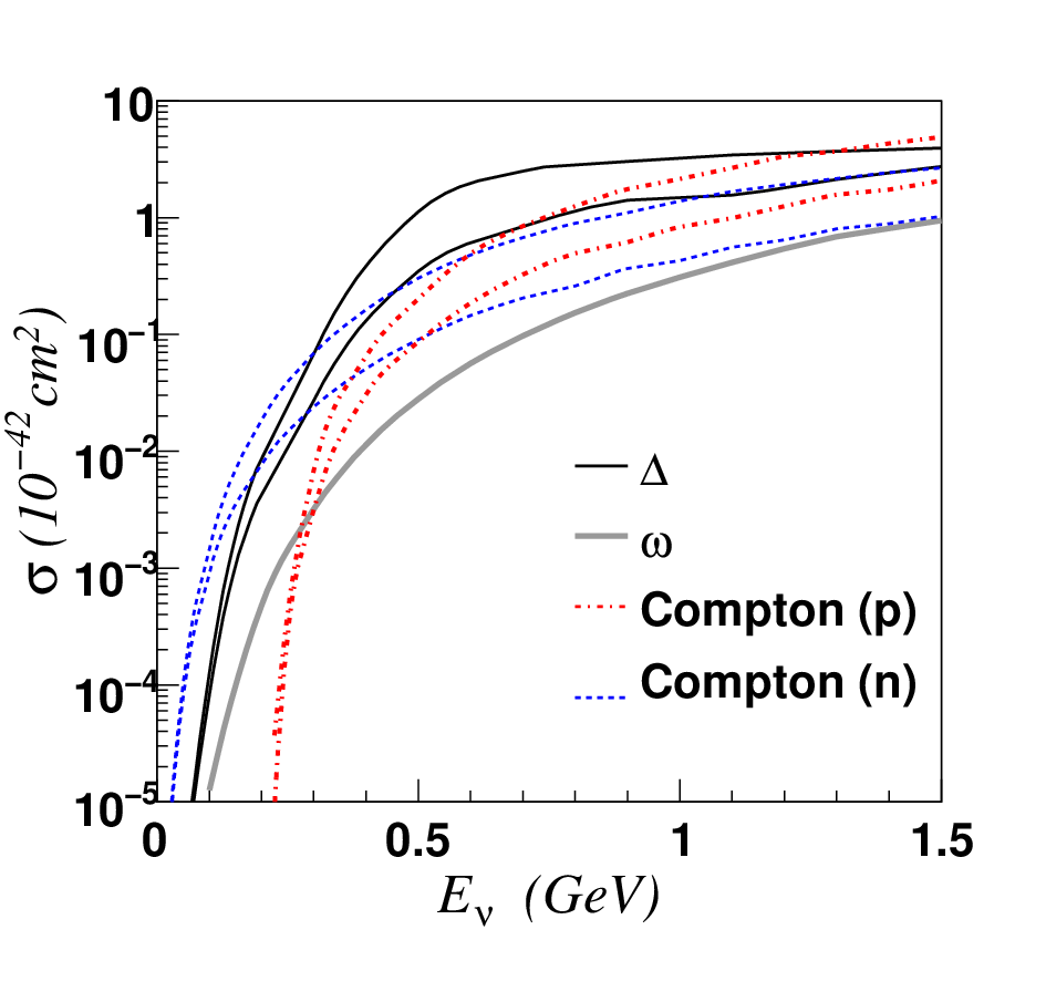
With all of the ingredients in place, it is straightforward to compute cross sections. This section provides a discussion of single-nucleon interactions, and the following section turns to coherent interactions involving compound nuclei.

Fig. 4 displays the various contributions to $\nu N\to\nu N\gamma$ including the effects of recoil of the final state nucleon, and the form factors specified in the previous section. The total Compton-like cross section for protons is divergent due to bremsstrahlung emission of soft photons. For illustration, the figure shows the total Compton-like cross section on protons for photon energy above $200\,{\rm MeV}$ . Since suppressed isovector contributions have been ignored in the meson exchange case, and since $\Delta$ resonance production results in pure isoscalar interactions, the remaining cross sections are the same for protons and neutrons.

At low energy, the cross sections reduce to the zero-recoil expressions derived earlier in (53) and (60)¹⁴¹⁴ 14 Recall that the $\omega$ and $\Delta$ contributions are of precisely the same form in this limit - we have neglected interference terms that would be important at very low energy. . In the zero-recoil limit there is no interference between vector and axial contributions in the Compton-like case, so that the cross sections for $\nu$ and $\overline{\nu}$ are identical in this limit. The operator describing $\omega$ and $\Delta$ channels at low energy involves only the axial-vector component of the weak hadronic current. The cross sections for these contributions are therefore also identical for $\nu$ and $\overline{\nu}$ in the zero-recoil limit. At large energy, interference between vector and axial-vector contributions yields a larger cross section for neutrinos over antineutrinos, except for the meson-exchange case where suppressed weak-vector contributions have been neglected.

Figure 5 displays partial cross sections as a function of photon energy, photon angle, and nuclear recoil $Q=[-(k-k^{\prime})^{2}]^{1/2}$ , for each of the $\omega$ -induced, $\Delta$ -induced and Compton-like cross sections. These representative results are for $E_{\nu}=1\,{\rm GeV}$ neutrinos scattering on protons.

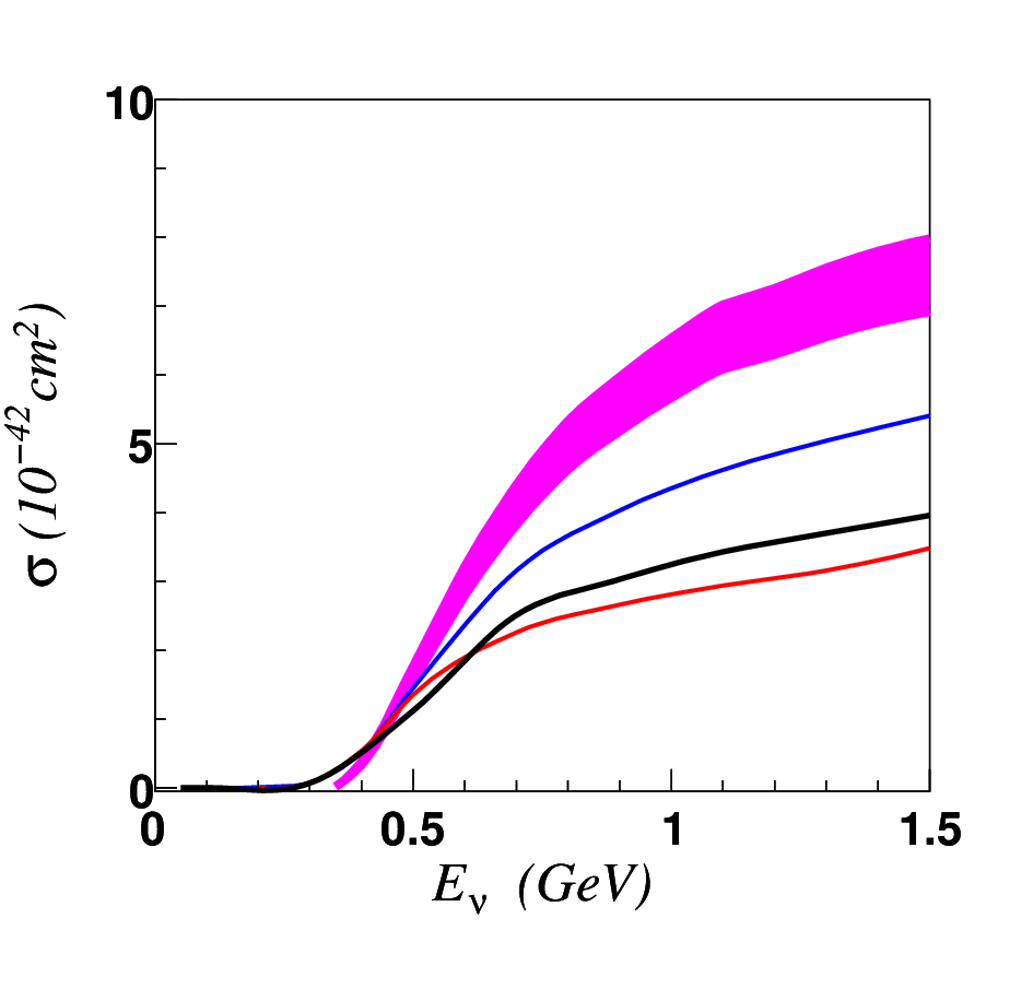
As an indication of uncertainties for the $\Delta$ contribution, Fig. 6 shows the cross section calculated with energy-dependent width (78); and using an alternate fit for the coefficients in (69): [21]

C^{A}_{5}=1.2\,,\quad C^{V}_{3}=2.13\,,\quad C^{V}_{4}=-1.51\,,\quad C^{V}_{5}=0.48\,.

(85)

The cross sections for offshell parameter $z=\pm 1$ in (72) are different by more than a factor of 2 at $E_{\nu}\to 0$ , as determined by (73). However, with the default form factor model and in the energy range considered, the total cross sections for $z=\pm 1$ differ by only a few percent above a few hundred MeV, where $\Delta$ can be produced onshell. The energy dependence of the width also has relatively minor impact on the total cross section above a few hundred MeV, suggesting that offshell effects do not impact GeV-scale cross sections dramatically. The spread in these curves in Fig. 6 can be taken as a crude estimate of the cross section uncertainty. Also displayed in Fig. 6 is the result obtained by multiplying the total cross section for $\nu N\to\nu\Delta$ (either $\nu p\to\nu\Delta^{+}$ or $\nu n\to\nu\Delta^{0}$ ) by the branching fraction $\sim 0.52-0.60$ [26] for $\Delta\to N\gamma$ . For this case, the $\Delta$ width is ignored, and the default form factors (69) are used¹⁵¹⁵ 15 The values for the total width and photon branching fraction obtained from form factors in (69) are $120\,{\rm MeV}$ and 0.42. For the form factors (85) the total width is unchanged and the photon branching fraction becomes 0.52. .

Corrections to the incoherent single-nucleon cross-sections from nuclear effects such as Fermi motion and Pauli blocking have been neglected. These considerations are not unique to single-photon production cross sections, and are beyond the scope of this paper. These effects should be incorporated in a more precise analysis, but are not expected to be dramatic for relatively large neutrino energies ( $E\sim 1\,{\rm GeV}$ ) on relatively small nuclei (e.g. ¹²C). The possibility of coherent processes, where the nucleus stays intact, is a distinct and interesting possibility. This is the subject of the following section.

V Coherence effects

In addition to interactions with individual nucleons, the weak and electromagnetic currents can scatter coherently off an entire nucleus. This section investigates the coherent contributions for each of the Compton-like, $\omega$ -induced and $\Delta$ -induced processes.

V.1 Compton scattering

The vector coupling of the $Z$ boson is primarily to the neutron, due to the smallness of the factor $1-4\sin^{2}\theta_{W}\approx 0.08$ appearing in the proton coupling. Of course, the vector photon couples directly only to the charged proton. Thus, the Compton-like cross section on either an isolated proton, or an isolated neutron, is smaller than naive power counting suggests. However, when coherent effects are considered, the $Z$ and photon couple to the total vector weak charge, and the total electric charge, respectively, and the charge suppressions are no longer effective. This process can be viewed as initial- and final-state radiation from the as-yet unobserved coherent neutral-current scattering of a neutrino from an intact, recoiling nucleus [27].

The scattering process can be described simply in the case of a spinless, isoscalar nucleus, e.g. ${\cal N}=^{12}$ C. Only isoscalar couplings are relevant, and the interactions with vector $Z$ and photon are described at low energy by an effective scalar field, with Lagrangian

{\cal L}=|D_{\mu}\phi|^{2}\,,

(86)

where the covariant derivative is

D_{\mu}\phi=\partial_{\mu}\phi-i\left(eQA^{\rm e.m.}_{\mu}+{g_{2}\over 2\cos\theta_{W}}Q_{W}Z_{\mu}\right)\phi\,.

(87)

The electric charge for an isoscalar nucleus is

Q=Z=\frac{1}{2}A\,,

(88)

and the weak vector charge is ( $Z=N=A/2$ )

Q_{W}=Z(\frac{1}{2}-2s_{W}^{2})+N(-\frac{1}{2})=-s_{W}^{2}A\,.

(89)

For the nonradiative process $\nu{\cal N}\to\nu{\cal N}$ , the cross section at low energy is calculated from (86) to be [27]

\sigma={1\over\pi}G_{F}^{2}A^{2}s_{W}^{4}E^{2}\,.

(90)

As the energy is increased, coherence becomes confined to the region of small momentum transfer, as implemented by including a form factor,

d\sigma\to d\sigma|F((k-k^{\prime})^{2})|^{2}\,.

(91)

Neglecting asymmetries in the neutron and proton distributions, this form factor should be the same as measured in electromagnetic scattering on the nucleus, $e^{-}{\cal N}\to e^{-}{\cal N}$ . The phenomenological form $F(t)=\exp(bt)$ is adopted, where for ¹²C we take $b\approx 25\,{\rm GeV}^{-2}$ [27]. In general nuclei, $b$ is expected to scale as $b\sim\langle r^{2}\rangle\sim A^{2/3}$ .

A straightforward calculation of the diagrams in Fig. 7 shows that the Compton-like cross section at very low energy is

{d\sigma\over dedx}={\alpha G_{F}^{2}E^{4}\sin^{4}\theta_{W}A^{2}\over 4\pi^{2}m_{N}^{2}}e(1-e)\left[{1\over e^{2}}\left(\frac{1}{2}-\frac{1}{6}x^{2}\right)+\frac{1}{e}\left(-\frac{7}{6}+\frac{5}{6}x^{2}\right)+\frac{4}{3}-\frac{2}{3}x^{2}-\frac{2}{3}e\right]\,.

(92)

In fact, this can be recognized as the cross section for a fermion of electric charge $F^{1}=Q$ , weak charge $C_{V}=Q_{W}$ and mass $Am_{N}$ , cf. (53). This should be true, since the low-energy electroweak probes cannot tell whether a single nucleon carries both $Q$ and $Q_{W}$ , or whether the charge is distributed over different nucleons. As the energy is increased, the coherent amplitude is again restricted to small momentum transfers. This is implemented by introducing the same form factor as above, so that the cross section is obtained by replacing the single-nucleon cross section by the ansatz

d\sigma(A)\approx A^{2}e^{2b(k-k^{\prime})^{2}}d\sigma(1)\,.

(93)

V.2 Virtual meson exchange

We have noted that $c^{(3)}_{4}$ in (25) describes the leading operator providing nuclear coherence for the axial-vector weak current. Neglecting nuclear modifications to the meson couplings, the coherent cross section induced by $\omega$ exchange at very low energy is simply $A^{2}$ times the single nucleon cross section (60). We again adopt a gaussian form factor, reflecting the distribution of nucleons inside the nucleus, and the cross section is modified from the single-nucleon case according to (93).

V.3 Coherent resonant production

When the photon energy is such that

m_{\Delta}^{2}-(k^{\prime}+q)^{2}\approx m_{\Delta}^{2}-m_{N}^{2}-2m_{N}E_{\gamma}\approx 0\,,

(94)

a resonant effect comes into play. Taking into account the finite width, the effect can be described by introducting a factor, for nonrelativistic nucleons,

	$\displaystyle{1\over(m_{\Delta}^{2}-m_{N}^{2})^{2}}$	$\displaystyle\to\left\|\frac{1}{2}{1\over m_{\Delta}^{2}-m_{N}^{2}-2m_{N}E_{\gamma}-i\Gamma_{\Delta}m_{\Delta}}+\frac{1}{2}{1\over m_{\Delta}^{2}-m_{N}^{2}+2m_{N}E_{\gamma}-i\Gamma_{\Delta}m_{\Delta}}\right\|^{2}$
		$\displaystyle={1\over(m_{\Delta}^{2}-m_{N}^{2})^{2}}\times{1+\gamma^{2}\over(1-\beta^{2}-\gamma^{2})^{2}+4\gamma^{2}}\,,$		(95)

where $\gamma=m_{\Delta}\Gamma_{\Delta}/(m_{\Delta}^{2}-m_{N}^{2})$ and $\beta=2m_{N}E_{\gamma}/(m_{\Delta}^{2}-m_{N}^{2})$ . The enhancement factor is plotted in Fig. 8. Coherence is again implemented by the ansatz (93).

The coherent aspect of the $s$ -channel $\Delta$ contribution can be understood as follows. In the limit $m_{\Delta},m_{N}\gg m_{\Delta}-m_{N}$ , the matrix elements can be calculated for nucleons at rest, and the leading interactions of the $N-\Delta$ system with vector and the axial-vector currents are proportional to the isovector magnetic moment operator. This can be seen explicitly by taking the nonrelativistic limit of the equation of motion derived from (62), leading to

i\epsilon^{ijk}\gamma^{j}\gamma_{5}\Delta^{a,k}\sim\Delta^{a,i}\,.

(96)

Thus for neutral fields, the hadronic part of the operators for $c^{(1)}_{N\Delta}$ and $c^{(2)}_{N\Delta,1}$ in (67) and (68) both involve $\overline{\Delta}^{a=3}_{i}N$ , plus terms suppressed by powers of $1/m_{N}$ . For each component of the external field (e.g. $A^{a,i}$ in (67), or $\epsilon^{ijk}F^{a,jk}$ in (68) ) the excitation $N\to\Delta$ occurs with fixed amplitude between a nucleon in a given spin state and a unique corresponding $\Delta$ spin state. The de-excitation $\Delta\to N$ obeys the same selection rule. For excitation by the weak neutral current, and de-excitation through the magnetic field, this leads to a $\bm{J}\cdot\bm{B}$ interaction coupled coherently to the nucleon. If the scattering takes place on a collection of nucleons, the final state cannot distinguish which nucleon was struck, giving rise to coherence.

An insightful model of the static nucleon transitions is obtained by viewing the baryons as solitonic “twisted” configurations of the pion field carrying unit baryon number. The solitonic description for large (odd) $N_{c}$ predicts a multiplet of low-lying baryons with spin and isospin $I=J=1/2,3/2,\dots,N_{c}/2$ . In particular for $N_{c}=3$ , the nucleon and $\Delta$ are singled out. The couplings of the baryons to external fields take a unique form, specified by the operators,

O^{i,a}={\rm Tr}(\tau^{i}a^{-1}\tau^{a}a)\,.

(97)

Here $a=a^{0}+\bm{a}\cdot\tau$ is an $SU(2)$ matrix field, and the baryon lagrangian is defined on the space of coordinates $\{a^{0},a^{1},a^{2},a^{3}\}$ . An explicit realization for the “potential” on this space of coordinates is the Skyrme model [28, 25], although many relations, such as properties following from the uniqueness of (97), are model-independent predictions of the large $N_{c}$ limit.

It is interesting to consider the coherent enhancement in terms of a simplified two-state model of the nucleon- $\Delta$ system. In this context, the excitation takes the ground state to a coherent superposition of singly-excited states for each of the $A$ nucleons,

|\downarrow\downarrow\downarrow\dots\rangle\to{1\over\sqrt{A}}\left(|\uparrow\downarrow\downarrow\dots\rangle+|\downarrow\uparrow\downarrow\dots\rangle+\dots\right)\,,

(98)

with amplitude proportional to $\sqrt{A}$ . Similarly, the amplitude for de-excitation and emission of a photon from this state is proportional to $\sqrt{A}$ . Hence the amplitude for the total process grows as $A$ , and the cross section as $A^{2}$ . This resonant coherent process has some relation to the “Dicke superradiance” effect encountered in atomic physics [29]¹⁶¹⁶ 16 I thank B. Adams for pointing out this reference. . However, in the language of spin systems, our spin $j=A/2$ system is prepared in $|j=A/2,j_{z}=-A/2+1\rangle$ . The true superradiant effect occurs when the system is somehow prepared in $|j=A/2,j_{z}\approx 0\rangle$ , due to the large coupling $\langle jj_{z}-1|\sigma_{-}|jj_{z}\rangle=\sqrt{(j+j_{z})(j-j_{z}+1)}\sim j\sim A$ for $j_{z}\sim 0$ (versus $\sqrt{A}$ for emission from the singly excited state). It would be amusing to consider whether such “nuclear superradiance” could be observed in practice, perhaps in some extreme astrophysical environment (it is certainly inefficient to induce multiple excitations by weak currents). It is also interesting to investigate the impact of density and temperature dependence of the $N-\Delta$ mass splitting.

V.4 Breakdown of coherence

Coherence is restricted to the case of momentum transfers that are small compared to the inverse size of the nucleus, with linear dimension $\sim A^{1/3}$ . For moderately sized nuclei, the naive $A^{2}$ scaling of the zero-recoil cross-sections is significantly modified already at hundreds of MeV incident neutrino energies. Before plotting the final cross sections, it is instructive to examine in some detail the limit of large energy, or large nucleus (specifically large $A^{2/3}E^{2}$ ) to see what remains of the coherent cross section.

To begin, we notice that the argument of the exponential factor in (93) may be expanded as

		$\displaystyle 2b(k-k^{\prime})^{2}=2b(p-p^{\prime}-q)^{2}=-4bE^{2}\left[(1-e)(1-y)+e(1-x)-e(1-e)(1-z)\right]$
		$\displaystyle\quad=-4bE^{2}\bigg\{(1-e)(\sqrt{1-x^{2}}\sqrt{1-z^{2}}+xz-y)+\frac{1}{2}[(1-e)\sqrt{1-z^{2}}-\sqrt{1-x^{2}}]^{2}$
		$\displaystyle\qquad+\frac{1}{2}[(1-e)(1-z)-(1-x)]^{2}\bigg\}\,,$		(99)

where $e=E_{\gamma}/E$ , $x=\cos\theta_{\gamma}=\hat{\bm{p}}\cdot\hat{\bm{q}}$ , $y=\hat{\bm{p}}\cdot\hat{\bm{p}}^{\prime}$ , $z=\hat{\bm{p}}^{\prime}\cdot\hat{\bm{q}}$ . This factor will be small when $\bm{p}^{\prime}+\bm{q}\approx\bm{p}$ , where the equality $|\bm{p}^{\prime}|+|\bm{q}|\approx|\bm{p}|$ is already enforced by the small-recoil limit. For this to happen, either $|\bm{q}|/|\bm{p}|=e$ or $|\bm{p}^{\prime}|/|\bm{p}|=1-e$ must be small, or the vectors must all be collinear. The overall size of the cross section then depends on the behavior of the remaining amplitude in these restricted regions of phase space.

The two cases of interest will be when $e\approx 0$ , or when both $e$ and $(1-e)$ are order unity. In the first case (soft photon), (99) reduces to

2b(k-k^{\prime})^{2}\approx-4bE^{2}(1-y)\approx-2bE^{2}\theta_{pp^{\prime}}^{2}\,.

(100)

which restricts the phase space to $\theta_{pp^{\prime}}\lesssim(bE^{2})^{-1/2}$ . In the remaining matrix element we can set $x\approx z$ and $y\approx 1$ .

In the second case (collinear photon), it is convenient to introduce $\theta^{\prime}$ , $\phi^{\prime}$ as polar and azimuthal angles of $\bm{p}^{\prime}$ with respect to $\bm{q}$ , where $\bm{p}$ and $\bm{q}$ define the x-z plane. Then $\sqrt{1-x^{2}}\sqrt{1-z^{2}}+xz-y=\sqrt{1-x^{2}}\sqrt{1-z^{2}}(1-\cos\phi^{\prime})$ , $\sqrt{1-x^{2}}=\sin\theta_{\gamma}$ and $\sqrt{1-z^{2}}=\sin\theta^{\prime}$ . Requiring that each of the three positive definite terms in (99) is not larger than order unity, the relevant region of phase space is

\phi^{\prime}\lesssim{(bE^{2})^{-1/2}\over(1-e)\theta^{\prime}}\,,\quad\theta-(1-e)\theta^{\prime}\lesssim(bE^{2})^{-1/2}\,,\quad\theta^{\prime}\lesssim{(bE^{2})^{-1/4}\over\sqrt{e(1-e)}}\,.

(101)

In the remaining matrix element we can set $x\approx y\approx z\approx 1$ . Retaining the $e$ dependence in (101) is not essential, but will allow us to indicate the leading behavior at $e\to 0$ and $e\to 1$ when e.g. $bE^{2}\ll e\to 0$ .

V.4.1 Compton-like process

Consider first the case of Compton-like scattering. The cross section is

\displaystyle{d\sigma({\rm Compton})\over dedx}

\displaystyle\propto A^{2}E^{4}e(1-e)\int d\cos\theta^{\prime}\int d\phi^{\prime}e^{2bE^{2}(k-k^{\prime})^{2}}\overline{\Sigma}|{\cal M}|^{2}\,,

(102)

where the spin-averaged matrix element is

\overline{\Sigma}|{\cal M}|^{2}\propto{1-e\over e^{2}}\big\{-2(1-e)y^{2}+y[-(1-e)^{2}z^{2}+2(1-e)xz-x^{2}-e^{2}+4(1-e)]\\ -(1-e^{2})z^{2}+2(1-e)xz-(1-2e)x^{2}+2(1-e)+e^{2}\big\}\,.

(103)

At small $bE^{2}$ , the gaussian factor can be neglected, and the integral over the final-state neutrino angle yields the result (92).

If we look for contributions at large $bE^{2}$ with $e$ and $1-e$ order unity, i.e., where both the photon and final-state neutrino carry a substantial fraction of the incoming neutrino energy, the relevant region of phase space is (101). Taking the appropriate limit of the matrix element,

\sigma({\rm Compton})\sim A^{2}E^{4}(bE^{2})^{-3/2}\int de{(1-e)^{2}\over e^{2}}\sim AE\int de{(1-e)^{2}\over e^{2}}\,.

(104)

For example, the partial cross section for photon carrying more than a fixed fraction of the incident neutrino energy scales as $AE$ , with the photon emitted in the forward direction.

In contrast, the partial cross section for photons in a fixed energy range corresponds to the case $e=E_{\gamma}/E\to 0$ . For this case, (100) applies, and the cross section becomes

{d\sigma({\rm Compton})\over dx}\sim A^{4/3}E^{2}\int{de\over e}\,.

(105)

The cross section for small-energy photons is dominant for large $bE^{2}$ , scaling as $A^{4/3}E^{2}$ . In this limit, the cross section is flat in photon angle, and logarithmically divergent for arbitrarily small photon energy.

V.4.2 $\omega$ and $\Delta$ processes

Moving next to the interaction induced by $\omega$ or $\Delta$ , the cross section takes the form (apart from a possible coherent enhancement depending on $e$ )

\displaystyle{d\sigma(\omega\,{\rm or}\,\Delta)\over dedx}

\displaystyle\propto A^{2}E^{6}e(1-e)\int d\cos\theta^{\prime}\int d\phi^{\prime}e^{2b(k-k^{\prime})^{2}}\overline{\Sigma}|{\cal M}|^{2}\,,

(106)

with

\overline{\Sigma}|{\cal M}|^{2}\propto e^{2}(1-e)(1-xz)\,.

(107)

Again, at small energy the gaussian factor can be ignored, and the integral over final-state neutrino angle yields a cross section of the form (60).

When the fractional energy, $e$ , carried by the photon goes to zero, (100) applies, and the cross section takes the form

{d\sigma(\Delta)\over dedx}\sim A^{2}E^{6}e^{3}(1-x^{2})\int dye^{-4bE^{2}(1-y)}\sim A^{4/3}E^{4}e^{3}(1-x^{2})\,.

(108)

For example, for the $\Delta$ contribution the photon energy is tied to the resonance mass, $e\sim(m_{\Delta}^{2}-m_{N}^{2})/2m_{N}E\to 0$ . Integrating over $e$ , the total cross section becomes independent of the incoming neutrino energy, and develops a $1-x^{2}$ angular dependence: $d\sigma/dx\sim A^{4/3}(1-x^{2})$ .

When both $e$ and $1-e$ are order unity (101) applies, and the cross section scales as

{d\sigma(\omega)\over de}\sim A^{2/3}E^{2}e[1+(1-e)^{2}]\,.

(109)

The photon is emitted in the forward direction, with energy spectrum tilted towards $e=1$ . At large nuclear size, the cross section grows as $A^{2/3}$ . This case is relevant to the $\omega$ exchange process, where the photon is able to carry an arbitrary fraction of the incoming neutrino energy.

Note that form factors in the vector or axial-vector channel of the weak current will induce an additional suppression involving powers of

[1-(p-p^{\prime})^{2}/m_{V,A}^{2}]^{-1}=[1+E^{2}(1-e)(1-y)/m_{V,A}^{2}]^{-1}\,.

(110)

In regions where $y\to 1$ (final-state neutrino collinear), this suppression is postponed to a higher scale. For example, for the $\omega$ process, we have $1-y\sim(bE^{2})^{-1/2}$ , so that the form factor cuts off energies above a mass scale parametrically of order $m_{\rm eff}\sim m_{A}^{2}b^{1/2}\sim A^{1/3}m_{A}^{2}/({1\,\rm GeV})$ . The restricted coherent cross section (109) grows more slowly than the number of nucleons $A$ , and hence more slowly as a function of $A$ than the incoherent process. However, the scale at which $E^{2}$ growth cuts off also becomes larger with $A$ .

From these considerations, the coherent cross sections are expected to behave very differently at large values of $bE^{2}$ . The total Compton-like process grows asymptotically as $A^{4/3}E^{2}\log{E/E_{\rm min}}$ above a threshold photon energy $E_{\rm min}$ , with photon energy spectrum weighted at the low end, and a flat distribution in photon angle. The $\Delta$ contribution saturates as a function of energy, and grows asymptotically with nuclear size as $A^{4/3}$ . The photon energy is fixed by the $\Delta$ excitation energy, and there is a $1-x^{2}$ photon angular distribution in the asymptotic limit. Finally, for the $\omega$ -mediated process, the growth with energy and nuclear size is $A^{2/3}E^{2}$ , and the process favors a forward photon carrying a large fraction of the incident neutrino energy. The $1\,{\rm GeV}$ energy range for a medium-sized nucleus like ${}^{12}C$ is in a transition region from small to large $bE^{2}$ , but the asymptotic limits are a useful guide for understanding the qualitative features of the coherent cross sections.

V.5 Summary of coherent single photon cross sections

The different components of the coherent cross section are depicted in Fig. 9. Distributions in photon energy and photon angle for $1\,{\rm GeV}$ incident neutrino energy are displayed in Fig. 10, for each of the Compton-like, $\Delta$ -induced and $\omega$ -induced neutrino cross sections. The upper limit of the band in Fig. 9 is obtained by combining the effects of $\omega$ and $\Delta$ into an effective coupling $g_{\omega}^{\rm eff}$ , and ignoring the resonant factor (95).

For $\Delta$ , inclusion of the subleading vector component of the weak current leads to a correction of the matrix element (107):

\overline{\Sigma}|{\cal M}|^{2}\propto e^{2}(1-e)\bigg\{1-xz\\ \pm{E\over m_{N}}{(1+a_{p}-a_{n})(1-2s_{W}^{2})\over 2g_{A}}\left[(2-e)(1-y)+(x-z)(x-(1-e)z)\right]+\dots\bigg\}\,,

(111)

where the $\pm$ refer to neutrino and antineutrino cross sections. Note that although $E$ is of order $1\,{\rm GeV}$ , the small-recoil condition enforced by the heavy nucleus ensures that the correction terms involve small momentum transfers. This leads to a suppression of the correction terms in both the soft (100) and collinear (101) limits.

The estimates presented here differ from previous calculations of coherent photon production in neutrino-nucleus scattering, which were focused at large energy. In [30], $A^{2}$ scaling was assumed at large energy, which is incorrect; the formulas presented there for the energy and angular distributions also do not have the correct low energy limit. In [31], the correct low-energy limit is not reproduced for contributions arising from the vector component of the weak neutral current. For example, the cross section does not reproduce the infrared singularity that must be present to describe bremsstrahlung emission. At higher energy, the strategy of relating the weak vector component of the cross section to the forward Compton amplitude is also problematic. The appearance of different isospin combinations for photon versus $Z^{0}$ couplings invalidates the assumption of a universal ratio of neutrino and photon cross sections mediated by different resonances. At low energy, this assumption is avoided in the present work by explicit consideration of the dominant ( $N$ , $\Delta$ ) intermediate states. The weak axial-vector cross section calculated in [31] corresponds roughly to the effects of our $t$ -channel $\omega$ exchange. However, the analogy used there between an effective $Z^{*}\gamma\gamma^{*}$ vertex [32] and a $Z^{*}\gamma\omega^{*}$ vertex is incorrect. In the former case ( $\gamma^{*}$ ), the amplitude must vanish when the $p^{2}$ of the photon goes to zero, due to gauge invariance and electromagnetic current conservation¹⁷¹⁷ 17 Equivalently, by the Landau-Yang theorem forbidding the decay of a massive vector into two identical massless vectors. . In the latter case ( $\omega^{*}$ ), the amplitude does not vanish as the $p^{2}$ carried by $\omega$ goes to zero, due to nonconservation of the baryon current. This is a reflection of the counterterm structure studied systematically in [1]. It turns out that (apart from a misplaced factor of $2$ in relating $\gamma N\to\pi^{0}N$ and the $\pi^{0}N\to\gamma N$ cross sections), their final cross section corresponds to the expression obtained here after integrating out $\omega$ . This results from a combined argument involving the (incomplete) $Z^{*}\gamma\gamma^{*}$ analogy and an appeal to PCAC [33]. The PCAC argument brings in further complications from $\pi^{0}$ absorption in the $\gamma N\to\pi^{0}N$ cross section, that are avoided by direct calculation. The axial-vector excitation of $\Delta(1232)$ is also omitted from [31], which is not justified in the GeV energy range.

V.5.1 Coherent single pion production

While it is not a focus of the present paper to explore the phenomenology of single pion production [34], this process is closely linked to that of single photon production. It is instructive to mention some of the similarities and differences that are encountered.

$\Delta$ should give the most prominent contribution to coherent single-pion production at low energies. Contributions to the matching condition (81) from effective scalar ( $\sigma$ ) degrees of freedom or from other excited nucleon states ( $N^{*}$ ) are subdominant, both from formal $1/N_{c}$ counting arguments, and from plausible numerical estimates [24]. In addition to this normalization, the $\Delta$ contribution leads to a resonant enhancement, in analogy to (95).

Compared to (111), the coherent single pion cross section mediated by $\Delta$ involves

\overline{\Sigma}|{\cal M}|^{2}\propto e^{2}(1-e)\bigg\{1-y+2xz\\ \pm{E\over m_{N}}{(1+a_{p}-a_{n})(1-2s_{W}^{2})\over g_{A}}\left[(2-e)(1-y)-(x-z)(x-(1-e)z)\right]+\dots\bigg\}\,.

(112)

In contrast to (111), Eq.(112) shows that the leading term for coherent pion production through the $\Delta$ resonance, $\propto 1-y+2xz$ , is not suppressed in the collinear limit. This, together with the relative minus sign in the two parts of the subleading term, implies a smaller difference in neutrino and antineutrino cross sections for coherent $\pi^{0}$ production compared to single photon production. (As already noted, the collinear region is not the dominant one at energies large compared to $(m_{\Delta}^{2}-m_{N}^{2})/2m_{N}\approx 300\,{\rm MeV}$ , mitigating the suppression of photon production.)

Let us make a few remarks on normalizing single photon production to $\pi^{0}$ production. If the cross sections for the two processes are related, measurement of the relatively abundant production of $\pi^{0}$ allows a constraint to be placed on the single photon process. For example, this procedure is used by the MiniBooNE collaboration to place bounds on single photon events as a background to $\nu_{e}$ appearance measurements [2, 35]. For incoherent scattering off individual nucleons, this procedure appears reasonable as a first approximation, provided the effects of pion reabsorption and rescattering can be accounted for. As indicated by Fig. 6 and the accompanying discussion, single photon production is not very sensitive to offshell modifications; roughly speaking, an onshell $\Delta(1232)$ is produced, and the relative number of single-photon and $\pi^{0}$ events should approximately follow the decay branching ratios of $\Delta\to N\pi^{0}$ and $\Delta\to N\gamma$ .

For the coherent interaction however, a number of complications enter into an attempt to normalize single-photon production to the $\pi^{0}$ rate. In contrast to the incoherent process, coherence enforces nontrivial constraints on the phase space for final-state particles, e.g. via the ansatz (93). Note that before the constraints are imposed, the total cross sections retain the relative normalization that would be predicted from the decay of an onshell $\Delta$ in the nonrelativistic limit¹⁸¹⁸ 18 The absolute normalization of the coherent cross section in the nonrelativistic limit corresponds to $2/3$ of the total cross section for $\nu p\to\nu\Delta^{+}$ , since there is a nonzero amplitude to flip the nucleon spin. . This can be verified by integrating (111) and (112) over the final-state phase space, $\int dx\,dy\,de\,e(1-e)$ (or $\int dx\,dz\,de\,e(1-e)$ ). Also in the soft limit (100) where $e\to 0$ , the normalization is still retained in the presence of the coherent form factor (93), as can be seen by taking $y=1$ , $x=z$ in (111) and (112), and integrating $\int dx$ . Note that the cross sections in this limit have very different distributions in phase space, with the photons distributed according to $1-x^{2}$ , and the pions distributed according to $2x^{2}$ .

Although the soft region dominates in the asymptotic $bE^{2}\to\infty$ limit, it is far from being precisely satisfied at $E\sim 1\,{\rm GeV}$ on relatively small (e.g. ¹²C) nuclei. In between the limits $bE^{2}\to 0$ and $bE^{2}\to\infty$ , the coherent single-photon and $\pi^{0}$ cross sections mediated by $\Delta$ are not simply related. The strong interaction of an emitted pion with the nucleus further complicates any simple comparison of $\pi^{0}$ and $\gamma$ production. Given these observations, with sufficient experimental data it may be useful to work in the opposite direction, i.e., to use the single-photon mechanism to isolate these effects, since the photon events do not suffer significant final-state interactions.

VI Summary and discussion

This paper surveyed single-photon production in neutrino-nucleon scattering in the $E_{\nu}\sim 1\,{\rm GeV}$ energy range. Several mechanisms come into play for both single-nucleon and coherent processes. At low energy, the effects are organized by a chiral lagrangian expansion, suitably extended to include the effects of general neutral electroweak gauge fields. For applications above a few hundred MeV, the effects of the dominant resonances in each channel were incorporated.

The results should provide a useful guide to the experimentalist dealing with single-photon signals and backgrounds. Several features of the analysis are also intriguing from a theoretical perspective. These include the notion of color-enhancement for the $\Delta$ -induced interaction; novel coherent-resonant phenomena reminiscent of the super-radiant effect in atomic physics; and the connection of the $\omega$ -induced interaction to the baryon current anomaly as noted in Ref. [3].

Single-photon events are an important background in experimental configurations such as MiniBooNE and T2K searching for $\nu_{e}$ appearance in a $\nu_{\mu}$ beam. This happens because a $\nu_{\mu}$ induced photon shower can be mistaken for the $\nu_{e}$ induced electron signal. Let us comment briefly on strategies to constrain these backgrounds. The $\Delta$ resonance plays a leading role. We noticed that the effects of uncertain offshell parameters are formally suppressed but have significant impact at low-energy. However, above several hundred MeV the rate of single photon production is found to be less sensitive to these offshell modifications. Thus, e.g., the procedure employed by MiniBooNE to normalize (incoherent) $\Delta\to N\gamma$ events in terms of the measured $\Delta\to N\pi^{0}$ rate appears reasonably justified as a first approximation, provided that $\pi^{0}$ absorption and rescattering effects can be reliably accounted for¹⁹¹⁹ 19 For related discussion on the issue of final-state pion interactions, see [35, 44]. . It would however be straightforward to calculate this rate directly, avoiding complications of the strongly-interacting pion inside the nucleus. Effects of Compton scattering and $t$ -channel $\omega$ exchange could likewise be simulated directly for the incoherent process.

The $\Delta$ resonance also plays a prominent role in the coherent process. Comparing to the analogous $\pi^{0}$ production is more difficult for this case. Besides the important effects of pion-nucleus interactions, the small- $Q^{2}$ constraints imposed by nuclear form factors blurs any simple relation between $\pi^{0}$ and $\gamma$ production. In particular, the $\gamma$ production will have a broader (less forward) angular distribution, and a larger vector-axial interference leading to a larger difference between $\nu$ and $\overline{\nu}$ cross sections. It appears that the $\omega$ -induced single-photon production plays a subdominant role at $\sim 1\,{\rm GeV}$ , being suppressed by form factors and recoil compared to naive estimates [3]. Interference effects between $\omega$ and $\Delta$ contributions will be significant at low energy where the respective amplitudes are described by the same effective operator. Note also that although the coherent $\Delta$ contribution saturates above $\sim 1\,{\rm GeV}$ , in our vector dominance model the $\omega$ contribution continues to grow as $E^{2}$ up to a parametrically larger scale, $E\sim A^{1/3}m_{\rm axial}^{2}/(1\,{\rm GeV})$ ; it may thus have a significant role to play at intermediate (few GeV) energies. Similarly, the correction to coherent $\pi^{0}$ production in (112) from $\omega$ becomes more significant at large energy. The Compton-like contribution to the coherent single-photon production was found to be small compared to the other mechanisms. It is interesting to note however that this process would provide an indirect means of observing coherent neutrino-nucleus scattering [27], via initial and final-state radiation.

It is interesting to consider whether new mechanisms of single photon production, in particular coherent processes, could explain an excess of events observed by MiniBooNE [35]. From Figs. 9 and 10, the $\Delta$ -induced component appears to be the largest effect; it is interesting that this component also has photon energy and angular distributions most closely resembling the excess. From the simple estimates presented here, the per-nucleon cross section for the coherent mechanism is similar in size to the incoherent case, and is not directly constrained by the analog $\pi^{0}$ production rate. In addition to this coherent-resonant effect, the $\omega$ -mediated process appears to be subdominant but non-negligible, and will add constructively to the $\Delta$ -mediated amplitude at low energy. Combined with the incoherent processes, and within large uncertainties, there appears to be a sufficient number of photons to cover the excess. More definitive statements would require further study of nuclear effects and detector efficiencies. It would be helpful to gather sufficient statistics to obtain cross sections for $\overline{\nu}N\to\overline{\nu}N\gamma$ [39]. Of course, distinguishing photon and electron events at the detector level would provide a decisive discrimination between different backgrounds. Similar cross sections should be measured by the T2K experiment. At lower energy, it is interesting to consider whether the analysis of signal events at the LSND experiment [40, 41] could have been influenced by a feed-down from decay-in-flight neutrinos that produce single photons.

It is interesting to pursue a more systematic classification in terms of invariant form factors for the general two-current electroweak matrix element. This would allow the definition of physical observables incorporating more information than the total cross sections. Such classification would generalize known results for the case of two vector currents (i.e. two photons) [38, 37, 36] to the case where one or both of the currents is axial-vector. In addition to enforcing constraints of discrete symmetries (parity and time reversal) and gauge invariance, a useful classification must account for the infrared singularities encountered in certain subprocesses. However, it is not obvious that such a classification would provide immediate physical insight, since an underlying dynamical model or small-parameter expansion is needed to parameterize both the normalization and shape of the invariant amplitudes²⁰²⁰ 20 For the case of real photon production from either the vector or axial-vector weak current, 12 invariant amplitudes correspond to the independent helicity amplitudes of $NZ^{*}\to N\gamma$ when the leptonic current is conserved, 16 when lepton masses are considered. . The present paper has instead focused on the systematic expansion of the chiral lagrangian at low energies, and used a phenomenological ansatz to perform a modest extrapolation into the GeV energy range. It would be interesting to investigate the invariant amplitudes in more detail and to look more systematically at higher energies. These aspects of formalism are beyond the scope of the present paper, but could be relevant to experiments with higher-energy neutrino beams. It is also interesting to consider the relevant interactions in the context of string-inspired models of QCD [42].

The relation between the baryon current anomaly and measurements of coherent photon interactions is more intricate than envisaged in Ref. [3], which motivated the present work. $\Delta$ and $\omega$ match onto the same effective operator at energies $E\ll m_{\omega},m_{\Delta}-m_{N}$ . The amplitudes constructively interfere, with $\Delta$ appearing to give a larger contribution. This clouds the intriguing connection between low-energy electroweak probes and the standard model baryon current anomaly. However, at the practical level, the effective coupling $g^{\rm eff}_{\omega}$ should be larger than considered in [3]. A more in-depth study of possible astrophysical applications is left to future work.

Acknowledgements

I thank J. Harvey and C. Hill for useful discussions and collaboration in the early stages of this work. This research was supported in part by the U.S. Department of Energy grant DE-AC02-76CHO3000.

Appendix A Compton amplitude to subleading order

This appendix presents the result of expanding the diagrams of Fig. 1 to subleading order in the $1/m_{N}$ expansion. This allows a direct comparison of the effects of the pCS operators to those of Compton scattering, as discussed after (51). Define:

{i\cal M}={-{ieg_{2}\over 2c_{W}}}\epsilon^{(\gamma)*}_{\mu}\epsilon^{(Z)}_{\nu}T^{\mu\nu}\,.

(113)

Working in units where $E_{\gamma}=q^{0}=1$ , the result is:

$\displaystyle T^{00}$	$\displaystyle=\frac{1}{m_{N}}\bigg[F_{1}C_{V}(2\bm{q}\cdot\bm{p})+F_{1}C_{A}(-2\bm{\sigma}\cdot\bm{q})\bigg]$
	$\displaystyle+\frac{1}{m_{N}^{2}}\bigg[F_{1}C_{V}\left(2\bm{q}\cdot\bm{p}\bm{q}\cdot(\bm{k}+\bm{k^{\prime}})-i\bm{\sigma}\cdot\bm{q}\times\bm{p}\right)+F_{1}C_{2}\left(-i\bm{\sigma}\cdot\bm{q}\times\bm{p}\right)$
	$\displaystyle\quad+F_{1}C_{A}\left(-\bm{q}\cdot\bm{p}\bm{\sigma}\cdot(\bm{k}+\bm{k^{\prime}})-\bm{q}\cdot(\bm{k}+\bm{k^{\prime}})\bm{\sigma}\cdot\bm{q}\right)+F_{2}C_{V}\left(-i\bm{\sigma}\cdot\bm{q}\times\bm{p}\right)\bigg]\,,$
$\displaystyle T^{i0}$	$\displaystyle=\frac{1}{m_{N}}\bigg[F_{1}C_{V}(2p^{i})+F_{1}C_{A}(-2\sigma^{i})\bigg]$
	$\displaystyle+\frac{1}{m_{N}^{2}}\bigg[F_{1}C_{V}\left(\bm{q}\cdot(\bm{k}+\bm{k^{\prime}})p^{i}+\bm{q}\cdot\bm{p}(k^{i}+k^{{}^{\prime}i})-i(\bm{p}\times\bm{\sigma})^{i}+i\bm{q}\cdot\bm{p}(\bm{q}\times\bm{\sigma})^{i}\right)$
	$\displaystyle\quad+F_{1}C_{2}\left(-i(\bm{p}\times\bm{\sigma})^{i}\right)+F_{1}C_{A}\left(-\bm{q}\cdot(\bm{k}+\bm{k^{\prime}})\sigma^{i}-p^{i}\bm{\sigma}\cdot(\bm{k}+\bm{k^{\prime}})\right)$
	$\displaystyle\quad+F_{2}C_{V}\left(-i(\bm{p}\times\bm{\sigma})^{i}+i\bm{q}\cdot\bm{p}(\bm{q}\times\bm{\sigma})^{i}\right)+F_{2}C_{A}\left((k^{i}+k^{{}^{\prime}i})\bm{q}\cdot\bm{\sigma}-\bm{q}\cdot(\bm{k}+\bm{k^{\prime}})\sigma^{i}\right)\bigg]\,,$
$\displaystyle T^{0j}$	$\displaystyle=\frac{1}{m_{N}}\bigg[F_{1}C_{V}(2q^{j})+F_{1}C_{A}(-2\bm{q}\cdot\bm{p}\sigma^{j})\bigg]$
	$\displaystyle+\frac{1}{m_{N}^{2}}\bigg[F_{1}C_{V}\left(\bm{q}\cdot\bm{p}(k^{j}+k^{{}^{\prime}j})+\bm{q}\cdot(\bm{k}+\bm{k^{\prime}})q^{j}+i(\bm{q}\times\bm{\sigma})^{j}-i\bm{p}\cdot\bm{q}(\bm{p}\times\bm{\sigma})^{j}\right)$
	$\displaystyle\quad+F_{1}C_{2}\left(-i\bm{q}\cdot\bm{p}(\bm{p}\times\bm{\sigma})^{j}+i(\bm{q}\times\bm{\sigma})^{j}\right)$
	$\displaystyle\quad+F_{1}C_{A}\left(-q^{j}\bm{\sigma}\cdot(\bm{k}+\bm{k^{\prime}})+(1-2\bm{q}\cdot\bm{p})\bm{q}\cdot(\bm{k}+\bm{k^{\prime}})\sigma^{j}\right)$
	$\displaystyle\quad+F_{2}C_{V}\left(i(\bm{q}\times\bm{\sigma})^{j}\right)+F_{2}C_{A}\left(i(\bm{q}\times\bm{p})^{j}+(k^{j}+k^{{}^{\prime}j})\bm{q}\cdot\bm{\sigma}-q^{j}(\bm{k}+\bm{k^{\prime}})\cdot\bm{\sigma}\right)\bigg]\,,$
$\displaystyle T^{ij}$	$\displaystyle=\frac{1}{m_{N}}\bigg[F_{1}C_{V}(2\delta^{ij})+F_{1}C_{A}\left(-2p^{i}\sigma^{j}+2(\delta^{ij}\bm{q}\cdot\bm{\sigma}-q^{j}\sigma^{i})\right)+F_{2}C_{A}\left(2(\delta^{ij}\bm{q}\cdot\bm{\sigma}-q^{j}\sigma^{i})\right)\bigg]$
	$\displaystyle+\frac{1}{m_{N}^{2}}\bigg[F_{1}C_{V}\big(i\epsilon^{ijr}\sigma^{r}(-1+\bm{p}\cdot\bm{q}-\bm{k}\cdot\bm{k^{\prime}})+k^{{}^{\prime}i}k^{{}^{\prime}j}-k^{i}k^{j}+k^{{}^{\prime}i}q^{j}+q^{i}k^{{}^{\prime}j}+q^{i}k^{j}+k^{i}q^{j}$
	$\displaystyle\quad+i\epsilon^{jrs}\sigma^{s}(-(k+k^{\prime})^{r}(k+k^{\prime})^{i}-p^{r}p^{i}+q^{r}q^{i})+i\epsilon^{irs}\sigma^{s}((k+k^{\prime})^{r}(k+k^{\prime})^{j}-p^{r}p^{j}+q^{r}q^{j})\big)$
	$\displaystyle\quad+F_{1}C_{2}\big(-i\epsilon^{ijr}\sigma^{r}+i\epsilon^{jrs}p^{r}(\delta^{is}\bm{\sigma}\cdot\bm{q}-p^{i}\sigma^{s}-q^{s}\sigma^{i})\big)$
	$\displaystyle\quad+F_{1}C_{A}\big(-(1-\bm{p}\cdot\bm{q})i\epsilon^{ijr}q^{r}-\delta^{ij}\bm{\sigma}\cdot(\bm{k}+\bm{k^{\prime}})+\bm{q}\cdot(\bm{k}+\bm{k^{\prime}})(q^{j}\sigma^{i}-\delta^{ij}\bm{q}\cdot\bm{\sigma})$
	$\displaystyle\qquad\qquad+\sigma^{j}(-\bm{q}\cdot(\bm{k}+\bm{k^{\prime}})q^{i}-2\bm{q}\cdot\bm{k^{\prime}}k^{{}^{\prime}i}+2\bm{q}\cdot\bm{k}k^{i})\big)$
	$\displaystyle\quad+F_{2}C_{V}\big(-i\epsilon^{ijr}\sigma^{r}+i\epsilon^{irs}q^{r}(-\delta^{sj}\bm{\sigma}\cdot\bm{p}+q^{j}\sigma^{s}+p^{s}\sigma^{j})\big)$
	$\displaystyle\quad+F_{2}C_{2}\big(2i\epsilon^{jrs}p^{r}(\delta^{is}\bm{\sigma}\cdot\bm{q}-q^{s}\sigma^{i})\big)$
	$\displaystyle\quad+F_{2}C_{A}\big((\bm{q}\cdot\bm{p}q^{r}-p^{r})i\epsilon^{ijr}+(k+k^{\prime})^{j}\sigma^{i}-\delta^{ij}(\bm{k}+\bm{k^{\prime}})\cdot\bm{\sigma}\big)\bigg]\,.$	(114)

The notation $C_{2}=F_{V}^{2\,,{\rm weak}}(0)$ is used. It is straightforward to check that $T^{00}=q^{i}T^{i0}$ and $T^{0j}=q^{i}T^{ij}$ as required by gauge invariance. For physical polarization states of the photon, we should take $\mu=i$ in (113). Interactions involving $C_{A}$ are then seen to be either spin-dependent, or vanish when $\bm{p}\to\bm{q}$ ; that is, they affect either the spin or the momentum of the struck nucleon.

References

[1] J. A. Harvey, C. T. Hill and R. J. Hill, “Standard Model Gauging of the Wess-Zumino-Witten Term: Anomalies, Global Currents and pseudo-Chern-Simons Interactions,” Phys. Rev. D 77, 085017 (2008) [arXiv:0712.1230 [hep-th]].
[2] A. A. Aguilar-Arevalo et al. [MiniBooNE Collaboration], Phys. Rev. Lett. 98, 231801 (2007).
[3] J. A. Harvey, C. T. Hill and R. J. Hill, “Anomaly mediated neutrino-photon interactions at finite baryon density,” Phys. Rev. Lett. 99, 261601 (2007) [arXiv:0708.1281 [hep-ph]].
[4] E. E. Jenkins and A. V. Manohar, Phys. Lett. B 255, 558 (1991).
[5] J. Gasser, M. E. Sainio and A. Svarc, Nucl. Phys. B 307, 779 (1988).
[6] S. Weinberg, Nucl. Phys. B 363, 3 (1991).
[7] V. Bernard, N. Kaiser and U. G. Meissner, Int. J. Mod. Phys. E 4, 193 (1995) [arXiv:hep-ph/9501384].
[8] S. R. Coleman, J. Wess and B. Zumino, “Structure of phenomenological Lagrangians. 1,” Phys. Rev. 177, 2239 (1969); C. G. . Callan, S. R. Coleman, J. Wess and B. Zumino, “Structure of phenomenological Lagrangians. 2,” Phys. Rev. 177, 2247 (1969). H. Georgi, “Weak Interactions And Modern Particle Theory,” Menlo Park, USA: Benjamin Cummings (1984) 165p.
[9] N. Fettes, U. G. Meissner and S. Steininger, Nucl. Phys. A 640, 199 (1998) [arXiv:hep-ph/9803266].
[10] For reviews of the large $N_{c}$ expansion applied to baryons see: E. Witten, Nucl. Phys. B 160, 57 (1979). A. V. Manohar, arXiv:hep-ph/9802419.
[11] V. Bernard, N. Kaiser and U. G. Meissner, Phys. Rev. D 50, 6899 (1994) [arXiv:hep-ph/9403351].
[12] C. H. Llewellyn Smith, Phys. Rept. 3, 261 (1972).
[13] A. A. Aguilar-Arevalo et al. [MiniBooNE Collaboration], Phys. Rev. Lett. 100, 032301 (2008) [arXiv:0706.0926 [hep-ex]].
[14] G. P. Lepage and S. J. Brodsky, Phys. Rev. D 22, 2157 (1980).
[15] R. Machleidt, K. Holinde and C. Elster, Phys. Rept. 149, 1 (1987).
[16] S. J. Barish et al., Phys. Rev. D 19, 2521 (1979).
[17] G. M. Radecky et al., Phys. Rev. D 25, 1161 (1982) [Erratum-ibid. D 26, 3297 (1982)].
[18] T. Kitagaki et al., Phys. Rev. D 34, 2554 (1986).
[19] T. Kitagaki et al., Phys. Rev. D 42, 1331 (1990).
[20] O. Lalakulich and E. A. Paschos, Phys. Rev. D 71, 074003 (2005) [arXiv:hep-ph/0501109].
[21] O. Lalakulich, E. A. Paschos and G. Piranishvili, Phys. Rev. D 74, 014009 (2006) [arXiv:hep-ph/0602210].
[22] V. Bernard, N. Kaiser and U. G. Meissner, Z. Phys. C 70, 483 (1996) [arXiv:hep-ph/9411287].
[23] G. Ecker, Phys. Lett. B 336, 508 (1994) [arXiv:hep-ph/9402337].
[24] V. Bernard, N. Kaiser and U. G. Meissner, Nucl. Phys. A 615, 483 (1997) [arXiv:hep-ph/9611253].
[25] G. S. Adkins, C. R. Nappi and E. Witten, Nucl. Phys. B 228, 552 (1983).
[26] C. Amsler et al. [Particle Data Group], Phys. Lett. B 667, 1 (2008).
[27] D. Z. Freedman, Phys. Rev. D 9, 1389 (1974).
[28] T. H. R. Skyrme, Proc. Roy. Soc. Lond. A 260, 127 (1961).
[29] R. H. Dicke, Phys. Rev. 93, 99 (1954).
[30] S. S. Gershtein, Yu. Y. Komachenko and M. Y. Khlopov, Sov. J. Nucl. Phys. 33, 860 (1981) [Yad. Fiz. 33, 1597 (1981)].
[31] D. Rein and L. M. Sehgal, Phys. Lett. B 104, 394 (1981) [Erratum-ibid. B 106, 513 (1981)].
[32] L. Rosenberg, Phys. Rev. 129, 2786 (1963).
[33] S. L. Adler, Phys. Rev. 135, B963 (1964).
[34] Coherent production has been considered in: N. G. Kelkar, E. Oset and P. Fernandez de Cordoba, Phys. Rev. C 55, 1964 (1997) [arXiv:nucl-th/9609005]. L. Alvarez-Ruso, L. S. Geng, S. Hirenzaki and M. J. Vicente Vacas, Phys. Rev. C 75, 055501 (2007) [arXiv:nucl-th/0701098]. D. Rein and L. M. Sehgal, Nucl. Phys. B 223, 29 (1983). A. A. Belkov and B. Z. Kopeliovich, Sov. J. Nucl. Phys. 46, 499 (1987) [Yad. Fiz. 46, 874 (1987)]. E. A. Paschos, A. Kartavtsev and G. J. Gounaris, Phys. Rev. D 74, 054007 (2006) [arXiv:hep-ph/0512139]. S. K. Singh, M. Sajjad Athar and S. Ahmad, Phys. Rev. Lett. 96, 241801 (2006).
[35] A. A. Aguilar-Arevalo et al. [MiniBooNE Collaboration], Phys. Rev. Lett. 102, 101802 (2009) [arXiv:0812.2243 [hep-ex]].
[36] R. Tarrach, Nuovo Cim. A 28, 409 (1975).
[37] M. Perrottet, Lett. Nuovo Cim. 7S2 (1973) 915 [Lett. Nuovo Cim. 7 (1973) 915].
[38] W. A. Bardeen and W. K. Tung, Phys. Rev. 173, 1423 (1968) [Erratum-ibid. D 4, 3229 (1971)].
[39] A. A. Aguilar-Arevalo et al., arXiv:0904.1958 [hep-ex].
[40] C. Athanassopoulos et al. [LSND Collaboration], Phys. Rev. Lett. 77, 3082 (1996) [arXiv:nucl-ex/9605003].
[41] C. Athanassopoulos et al. [LSND Collaboration], Phys. Rev. Lett. 81, 1774 (1998) [arXiv:nucl-ex/9709006].
[42] S. K. Domokos and J. A. Harvey, Phys. Rev. Lett. 99, 141602 (2007).
[43] T. R. Hemmert, B. R. Holstein and J. Kambor, J. Phys. G 24, 1831 (1998) [arXiv:hep-ph/9712496].
[44] T. Leitner, O. Buss, U. Mosel and L. Alvarez-Ruso, PoS NUFACT08, 009 (2008) [arXiv:0809.3986 [nucl-th]].

Low energy analysis of ν​N→ν​N​γ\nu N\to\nu N\gamma in the Standard Model