Optimal Embedding Into Star Metrics
Abstract
We present an -time algorithm for the following problem: given a finite metric space , create a star-topology network with the points of as its leaves, such that the distances in the star are at least as large as in , with minimum dilation. As part of our algorithm, we solve in the same time bound the parametric negative cycle detection problem: given a directed graph with edge weights that are increasing linear functions of a parameter , find the smallest value of such that the graph contains no negative-weight cycles.
1 Introduction
A metric space is a set of sites separated by symmetric positive distances that obey the triangle inequality. If and are metric spaces and does not decrease the distance between any two points, the dilation or stretch factor of is
We define a star metric to be a metric space in which there exists a hub such that, for all and , . Given the distance matrix of an -point metric space , we would like to construct a function that maps into a star metric , that does not decrease distances, and that has as small a dilation as possible. In this paper we describe an algorithm that finds the optimal in time . Our problem may be seen as lying at the confluence of three major areas of algorithmic research:
Spanner construction. A spanner for a metric space is a graph with the points of as its vertices and weights (lengths) on its edges, such that path lengths in equal or exceed those in ; the dilation of is measured as above as the maximum ratio between path length and distance in . The construction of sparse spanners with low dilation has been extensively studied [9] but most papers in this area limit themselves to bounding the dilation of the spanners they construct rather than constructing spanners of optimal dilation. Very few optimal spanner construction problems are known to be solvable in polynomial time; indeed, some are known to be NP-complete [15] and others NP-hard [3, 8]. Our problem can be viewed as constructing a spanner in the form of a star (a tree with one non-leaf node) that has optimal dilation.
Metric embedding. There has been a large amount of work within the algorithms community on metric embedding problems, in which an input metric space is to be embedded into a simpler target space with minimal distortion [16]; typical target spaces for results of this type include spaces with norms and convex combinations of tree metrics. As with spanners, there are few results of this type in which the minimum dilation embedding can be found efficiently; instead, research has concentrated on proving bounds for the achievable dilation. Our result provides an example of a simple class of metrics, the star metrics, for which optimal embeddings may be found efficiently. As with embeddings into low-dimensional spaces, our technique allows an input metric with a quadratic number of distance relationships to be represented approximately using only a linear amount of information.
Facility location. In many applications one is given a collection of demand points in some space and must select one or more supply points that maximize some objective function. For instance, the 1-median (minimize the sum of all distances from demand points to a single supply point) and 1-center (minimize the greatest distance between any destination point and a single supply point) can be applied to operational challenges such as deciding where to build a radio transmitter or railroad hub so as to maximize its utility [7]. In a similar vein the problem discussed in this paper may be seen as selecting a single supply point to serve as the hub of a star-topology network. In this context dilation corresponds to the worst multiplicative cost penalty imposed on travel between any pair of input points due to the requirement that all travel is routed through the hub (center) point. Superficially, our problem differs somewhat from typical facility location problems in that the star we construct has a hub that is not given as part of the input. However, it is possible to show that the hub we find belongs to the tight span of the input metric space [6], a larger metric space that has properties similar to those of spaces. Viewing our problem as one of selecting the optimal hub point from the tight span gives it the format of a facility location problem.
Previously [10] we considered similar minimum dilation star problems in which the input and output were both confined to low-dimensional Euclidean spaces. As we showed, the minimum-dilation star with unrestricted hub location may be found in expected time in any bounded dimension, and for the optimal hub among the input points may be selected in expected time , where is the inverse Ackermann function. For the general metric spaces considered here, the difficulty of the problems is reversed: it is trivial to select an input point as hub in time , while our results show that an arbitrary hub may be found in time .
As we discuss in Section 2, the minimum dilation star problem can be represented as a linear program; however solving this program directly would give a running time that is a relatively high order polynomial in and in the number of bits of precision of the input matrix. In this paper we seek a faster, purely combinatorial algorithm whose running time is strongly polynomial in . Our approach is to first calculate the dilation of the optimal star. We do this by forming a -graph : a directed graph with weights in the form for parameters and determined from the input metric. has the property that it contains no negative weight cycles if and only if there exists a star with dilation . Next we calculate , the smallest value such that contains no negative-weight cycles, which is also the dilation of the star we will eventually create. Finally we use and to compute the lengths of the edges from the star’s center to each site, and output the resulting star.
Our algorithm for computing , the smallest parameter value admitting no negative cycles in a parametrically weighted graph, warrants independent discussion. To our knowledge no known strongly polynomial algorithm solves this problem in full generality. Karp and Orlin [14] gave an time algorithm for a problem in which the edge weights have the same form as ours, but where each is restricted to the set . If all , the problem is equivalent to finding the minimum mean cycle in a directed graph [13], for which several algorithms run in time [4]. In our problem, each may be any nonnegative real number; it is not apparent how to adapt the algorithm of Karp and Orlin to our problem. Gusfield provided an upper bound [12] on the number of breakpoints of the function describing the shortest path length between two nodes in a -graph, and Carstensen provided a lower bound [2] for the same quantity; both bounds have the form . Hence any algorithm that constructs a piecewise linear function that fully describes path lengths for the entire range of values takes at least time. In Section 4 we describe our algorithm, which is based on a dynamic programming solution to the all pairs shortest paths problem. Our algorithm maintains a compact piecewise linear function representing the shortest path length for each pair of vertices over a limited range of values, and iteratively contracts the range until a unique value can be calculated. Thus it avoids Carstensen’s lower bound by finding only the optimal , and not the other breakpoints of the path length function, allowing it to run in time.
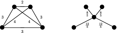
2 Linear Programming Formulation
In this section we formally define the overall minimum dilation star problem and describe how to solve it directly using linear programming. Our eventual algorithm never solves nor even constructs this linear program directly; however stating the underlying linear program and its related terminology will aid our later exposition.
The input to our algorithm is a finite metric space. Formally, a metric space is a tuple , where is a set of sites and the function maps any pair of sites to the nonnegative, real distance between them. The following metric conditions also hold for any :
- 1.
if and only if (positivity);
- 2.
(symmetry); and
- 3.
(the triangle inequality).
The input to our algorithm is a finite metric space ; we assume that the distance between any may be reported in constant time, for instance by a lookup matrix.
A star is a connected graph with one center vertex. A star contains an edge between the center and every other vertex, but no other edges. Hence any star is a tree of depth 1, and every vertex except the center is a leaf. Our algorithm must output a weighted star whose leaves are the elements from the input. The edge weights in must be at least as large as the distances in , and must obey reflexivity and the triangle inequality. In other words, if is the length of a shortest path from to in , then , , and for any vertices in .
We also ensure that the dilation of is minimized. For any two vertices in some weighted graph whose vertices are points in a metric space, the dilation between and is
The dilation of the entire graph is the largest dilation between any two vertices, i.e.
Our output graph is a star; hence every path between two leaves has two edges, so if we apply the definition of dilation to , we obtain
where is the weight of the edge connecting and in . Hence the dilation of may be computed by
This equation lays the foundation for our formulation of the minimum dilation star problem as a linear program.
Definition 1
Let be the following linear program, defined over the variables and for every :
Minimize
such that for any ,
| (1) |
and for any ,
| (2) | |||||
| (3) |
Let be the value assigned to in the optimal solution to . In other words, is the smallest dilation admitted by any set of distances satisfying all the constraints of .
is clearly feasible. For example, if , then the solution and is a feasible, though poor, solution.
Lemma 1
For any optimal solution of , the value of gives the minimum dilation of any star network spanning , and the values give the edge lengths of an optimal star network spanning .
Proof
Each variable corresponds to the weight of the edge between and in . Inequality 1 ensures that the distances are nonnegative, Inequality 2 ensures that they obey the triangle inequality, and Inequality 3 dictates that is a largest dilation among any pair of sites from . The value of is optimal since is defined to minimize .
Unfortunately contains variables and constraints. Such a program could be solved using general purpose techniques in a number of steps that is a high-order polynomial in and the number of bits of precision used, but our objective is to obtain a fast algorithm whose running time is strongly polynomial in . Megiddo showed [19] that linear programs with at most two variables per inequality may be solved in strongly polynomial time; however our type (3) inequalities have three variables, so those results cannot be applied to our problem.
3 Reduction to Parameteric Negative Weight Cycle Detection
In this section we describe a subroutine that maps the set of sites to a directed, parametrically-weighted -graph . Every edge of is weighted according to a nondecreasing linear function of a single graph-global variable . An important property of is that the set of values of that cause to contain a negative weight cycle is identical to the set of values of that cause the linear program to be infeasible. Thus any assignment of for which contains no negative weight cycles may be used in a feasible solution to .
Definition 2
A -graph is a connected, weighted, directed graph, where the weight of any edge is defined by a linear function in the form
where and are real numbers and .
Definition 3
Let be the -graph corresponding to a particular set of input sites . has vertices and for each . For , has an edge of length from to , and for , has an edge of length from to .
Note that an edge from to has weight when . An example -graph for is shown in Figure 2.

Lemma 2
may be constructed in time.
Proof
has vertices and edges, each of which may be initialized in constant time.
Lemma 3
If is assigned such that has a feasible solution, then contains no negative weight cycle.
Proof
Since is bipartite, any sequence of edges traversed by a cycle in has even length. Depending on which partition begins with, the sequence either takes the form
or
where are vertices from . In either case, the cycle has weight
| (4) |
by the commutativity of addition. Since is feasible, there exists some set of distances satisfying the constraints of , i.e.
| (5) |
and
| (6) |
Substituting (5) and (6) into (4), we obtain
Theorem 3.1
Any set of sites from a metric space may be mapped to a -graph with vertices, such that for any , contains a negative weight cycle if and only if is infeasible for that value of . The mapping may be accomplished in time.
Proof
By Lemma 2, may be created in time, and by Lemma 3, feasibility of implies an absence of negative cycles in . Section 5 describes an algorithm that, given a value for which has no negative cycle, generates an edge length for every that obeys the constraints of . Thus, by the correctness of that algorithm, an absence of negative cycles in implies feasibility of .
4 Searching for
We now turn to the problem of computing the quantity . This problem is an example of parametric negative weight cycle detection: given a -graph , find , the smallest value such that contains no cycles of negative weight. Our algorithm functions by maintaining a range which is known to contain . Initially the range is ; over iterations, the range is narrowed until it is small enough that may be calculated easily. This approach is similar in spirit to Megiddo’s general parametric search framework [17, 18], which, in loose terms, searches for the solution to an optimization problem by simulating the execution of a parallel algorithm for the corresponding decision problem.
Our algorithm is presented in Listing 1. It is an adaptation of a parallel all pairs shortest paths algorithm based on matrix squaring [20]. The original algorithm uses a matrix , which stores the weight of the shortest path from to among paths with at most edges. Each may be defined as the smallest sum of two cells of , and defines the shortest paths in the graph. In the context of that original algorithm, edges and paths had real-number lengths, so it was sufficient to store real numbers in . In the context of this paper, an edge’s weight is a linear function of a variable ; hence the weight of a path is a linear function of . Unfortunately the minimum-cost path between and may be different for varying values of , so the weight of the shortest path from to is defined by the minima of one or more linear functions of . Such a lower envelope of linear functions may be represented by a piecewise linear function; hence each element of must store a piecewise linear function. Without further attention the number of breakpoints in these piecewise linear functions would grow at every iteration, and eventually operating on them would dominate our algorithm’s running time. To address this, at every iteration we choose a new interval that contains no breakpoints, so that every may be compacted down to a single linear function.
Lemma 4
For any , the function as computed in the listing evaluates to the weight of the shortest path from to among paths with at most edges, or if no such path exists.
Proof
We argue by induction on . In the base case , must represent the weight of shortest path from to that includes up to edges. The only such paths are trivial paths, for which and , and single edge paths, for which the path length equals the edge length.
For , each is first defined as the lower envelope of two entries of in line 10, then redefined as a strictly linear function over the new smaller range in line 16, so we argue that the lemma holds after each assignment. In the first assignment, is defined to be the lower envelope of for all ; in other words, every is considered as a potential “layover” vertex, and is defined as a piecewise linear function that may be defined by differing layover vertices throughout the range . By the inductive hypothesis, the values represent weights of minimum cost paths with at most edges; hence the resulting values represent weights of minimum cost paths with at most edges.
When is reassigned in line 16, the range endpoints and have been contracted such that no entry of contains breakpoints in the range . Hence any individual has no breakpoints in that range, and is replaced by a simple linear function. This transformation preserves the condition that represents the weight of the shortest path from to for any .
Lemma 5
Given two values and such that , it is possible to decide whether , , or , in time.
Proof
By Lemma 3, for any value , if contains a negative cycle when , then . So we can determine the ordering of , and using the Bellman–Ford shortest paths algorithm [1, 11] to detect negative cycles, as follows. First run Bellman–Ford, substituting to evaluate edge weights. If we find a negative cycle, then report that . Otherwise run Bellman–Ford for ; if we find a negative cycle, then must be in the range . If not, then . This decision process invokes the Bellman–Ford algorithm once or twice, and hence takes time.
Lemma 6
The algorithm presented in Listing 1 runs in time.
Proof
Each is a linear function, so each is a linear function as well. is defined as the lower envelope of such linear functions, which may be computed in time [5]. So each may be computed is time, and all iterations of the first inner for loop take total time. Each represents the lower envelope of lines, and hence has breakpoints. So the entries of contain a total of breakpoints, and they may all be collected and sorted into in time. Once sorted, any duplicate elements may be removed from in time.
Next our algorithm searches for a new, smaller range that contains . Recall that is the value of for which contains no negative weight cycle, and every entry of is a piecewise linear function comprised of non-decreasing linear segments; so it is sufficient to search for the segment that intersects the line. We find this segment using a binary search in . At every step in the search, we decide which direction to seek using the decision process described in Lemma 5. Each decision takes time, and a binary search through the elements of makes decisions, so the entire binary search takes time.
Replacing an entry of with a (non-piecewise) linear function may be done naively in time by scanning the envelope for the piece that defines the function in the range . So the second inner for loop takes total time, and the outer for loop takes a total of time.
The initialization before the outer for loop takes time. The last step of the algorithm is to compute , the smallest value in the range such that for every . At this point each is a non-piecewise increasing linear function, so this may be done by examining each of the linear functions , solving for its -intercept, and setting to be the largest intercept. This entire process takes time, so the entire algorithm takes time.
Theorem 4.1
The algorithm presented in Listing 1 calculates in time.
5 Extracting the Edge Weights
Once has been calculated, all that remains is to calculate the weight of every edge in the output star. Our approach is to create a new graph , which is a copy of with the addition of a new source node with an outgoing weight 0 edge to every (see Figure 3). We then compute the single source shortest paths of starting at , and define each to be a function of the shortest path lengths to and . This process is a straightforward application of the Bellman–Ford algorithm, and hence takes time. The remainder of this section is dedicated to proving the correctness of this approach.

Definition 4
Let be a copy of the graph described in Definition 3, with all edge weights evaluated to real numbers for , and the addition of a source vertex with an outgoing 0-weight edge to every . Let be a shortest path from to for any vertex , and let be the total weight of any such . The operation yields the path formed by appending the edge to .
Definition 5
Define
We now show that our choice of satisfies all three metric space properties.
Lemma 7
Every satisfies .
Proof
For each vertex there exists an edge from to with weight 0.
Lemma 8
Every distinct and satisfy
Proof
By the definition of shortest paths, we have
and by symmetric arguments,
Adding these inequalities, we obtain
Lemma 9
Every distinct and satisfy
Proof
Observe that the path is a path to with weight , and that the path is a path to with weight . By definition is a shortest path to , and similarly is a shortest path to , so we have
and
Adding these inequalities, we obtain
By assumption , so
Theorem 5.1
Given and the corresponding and , a set of edge lengths for each , such that for every
and for every distinct
may be computed in time.
6 Conclusion
Finally we codify the main result of the paper as a theorem.
Theorem 6.1
Given a set of sites from a metric space , it is possible to generate a weighted star such that the distances between vertices of obey the triangle inequality, and such that has the smallest possible dilation among any such star, in time.
Acknowledgements
This work was supported in part by NSF grant 0830403 and by the Office of Naval Research under grant N00014-08-1-1015.
References
- [1] R. Bellman. On a routing problem. Quarterly in Applied Mathematics, 16(1):87–90, 1958.
- [2] P. J. Carstensen. Parametric cost shortest chain problem. Manuscript, Bellcore, 1984.
- [3] O. Cheong, H. Haverkort, and M. Lee. Computing a minimum-dilation spanning tree is NP-hard. In Proc. 13th Australasian Symp. Theory of Computing, pages 15–24, 2007.
- [4] A. Dasdan, S. Irani, and R. Gupta. An experimental study of minimum mean cycle algorithms. Technical report, University of California, Irvine, 1998.
- [5] M. de Berg, M. van Kreveld, M. Overmars, and O. Schwarzkopf. Computational Geometry: Algorithms and Applications. Springer-Verlag, 2nd edition, 1998.
- [6] A. W. M. Dress, K. T. Huber, and V. Moulton. Metric spaces in pure and applied mathematics. In Proc. Quadratic Forms LSU, Documenta Mathematica, pages 121–139, 2001.
- [7] Z. Drezner and H. Hamacher. Facility Location: Applications and Theory. Springer, 2002.
- [8] J. Edmonds. Embedding into is Easy, Embedding into is NP-Complete. Discrete and Computational Geometry, 39(4):747–765, June 2008.
- [9] D. Eppstein. Spanning trees and spanners. In J.-R. Sack and J. Urrutia, editors, Handbook of Computational Geometry, chapter 9, pages 425–461. Elsevier, 2000.
- [10] D. Eppstein and K. A. Wortman. Minimum dilation stars. Computational Geometry, 37(1):27 – 37, 2007. Special Issue on the Twenty-First Annual Symposium on Computational Geometry - SoCG 2005.
- [11] L. R. Ford and D. Fulkerson. Flows in Networks. Princeton University Press, 1962.
- [12] D. Gusfield. Sensitivity analysis for combinatorial optimization. Technical Report UCB/ERL M80/22, Electronics Research Laboratory, Berkeley, 1980.
- [13] R. M. Karp. A characterization of the minimum cycle mean in a digraph. Discrete Mathematics, 23(3):309–311, 1978.
- [14] R. M. Karp and J. B. Orlin. Parametric Shortest Path Algorithms with an Application to Cyclic Staffing. Technical Report OR 103-80, MIT Operations Research Center, 1980.
- [15] R. Klein and M. Kutz. Computing geometric minimum-dilation graphs Is NP-hard. In Proc. 14th Int. Symp. Graph Drawing, volume 4372 of Lecture Notes in Computer Science, pages 196–207, 2007.
- [16] N. Linial. Finite metric spaces–combinatorics, geometry and algorithms. In Proc. International Congress of Mathematicians, Beijing, volume 3, pages 573–586, 2002.
- [17] N. Megiddo. Combinatorial optimization with rational objective functions. In Proc. 10th ACM Symp. Theory of computing, pages 1–12. ACM, 1978.
- [18] N. Megiddo. Applying Parallel Computation Algorithms in the Design of Serial Algorithms. J. ACM, 30(4):852–865, 1983.
- [19] N. Megiddo. Towards a Genuinely Polynomial Algorithm for Linear Programming. SIAM Journal on Computing, 12(2):347–353, 1983.
- [20] C. Savage. Parallel Algorithms for Graph Theoretic Problems. PhD thesis, University of Illinois, Urbana-Champaign, 1977.