Ratios of maximal concurrence-parameterized separability functions, and generalized Peres-Horodecki conditions
Abstract
The probability that a generic real, complex or quaternionic two-qubit state is separable can be considered to be the sum of three contributions. One is from those states that are absolutely separable, that is those (which can not be entangled by unitary transformations) for which the maximal concurrence over spectral orbits () is zero. The other two contributions are from the states for which , and for which . We have previously (arXiv:0805.0267) found exact formulas for the absolutely separable contributions in terms of the Hilbert-Schmidt metric over the quantum states, and here advance hypotheses as to the exact contributions for . A crucial element in understanding the two contributions for is the nature of the ratio () of the -parameterized separability function for the complex states to the square of the comparable function for the real states–both such functions having clearly displayed jump discontinuities at . For , the ratio appears to be of the form , except near , while for , there is strong numerical evidence that it equals 2 (thus, according to the Dyson-index pattern of random matrix theory). Related phenomena also occur for the minimally-degenerate two-qubit states and the qubit-qutrit states. Our results have immediate application to the computation of separability probabilities in terms of other metrics, such as the Bures (minimal monotone) metric. The paper begins with continuous embeddings of the separability probability question in terms of four metrics of interest, using ”generalized Peres-Horodecki conditions”.
Mathematics Subject Classification (2000): 81P05; 52A38; 15A90; 28A75
Keywords:
eigenvalues, , two qubits, separability probabilities, Euler-angle parameterization, quasi-Monte Carlo, numerical integration, Hilbert-Schmidt metric, Bures metric, minimal monotone metric, Wigner-Yanase metric, Kubo-Mori metric, quasi-Bures metric, concurrence, maximal concurrence, Dyson indices, random matrix theorypacs
Valid PACS 03.67.Mn, 02.30.Cj, 02.40.Ky, 02.40.FtI Introduction
One possibly productive strategy to pursue when confronted with an apparently intractable problem, is to embed it in some broader class of problems. Doing so, hopefully, may lead to new insights and progress, including ones regarding the original (smaller) problem. In the first of the two basic parts of this paper (secs. II-VII), we adopt such embedding strategies for the task of determining the probabilities–with regard to a number of metrics of quantum-mechanical interest–that certain generic forms of or quantum system are separable [1, 2, 3, 4, 5, 6, 7, 8]. (As computers presumably grow more powerful, these readily-formulated, but high-dimensional [9, 15, …] and high-degree [e. g., quartic] problems may eventually lose their apparent present-day intractability (cf. [9, 10])–much as did the famous four-color planar map theorem of Appel and Haken [11, 12]. Nevertheless, it would certainly be appealing to address these problems with more theoretical understanding than is required by ”brute force” computation (cf. [13, 14, 15, 16]).)
In the second basic part (secs. VIII-X), building upon our recent work in [17], we attempt to gain insight–using manifest relations to random matrix theory–into the very same separability probability questions by determining the nature of certain eigenvalue-parameterized separability functions. These are expressed as univariate functions of the maximal concurrence over spectral orbits.
The fundamental question being addressed here of determining the probability that a generic bipartite quantum state is separable or not was first raised by Życzkowski, Horodecki, Sanpera and Lewenstein in a pioneering, much-cited 1998 paper [1]. As motivation they wrote: ”One of the fundamental questions concerning these subjects is to estimate how many entangled (disentangled) states exist among all quantum states. More precisely, one can consider the problem of quantum separability or inseparability from a measurement theoretical point of view, and ask about relative volumes of both sets. There are three main reasons of importance in this problem. The first reason, of some philosophical implication, may be contained in the questions ÔÔIs the world more classical or more quantum? Does it contain more quantum-correlated (entangled) states than classically correlated ones?ÕÕ The second reason has a more practical origin. Analyzing some features of entanglement, one often has to rely on numerical simulations. It is then important to know to what extent entangled quantum states may be considered as typical. Finally, the third reason has a physical origin. The physical meaning of separability has recently been associated with the possibility of partial time reversal” [1, p. 883].
In sec. II, in the first basic part of the paper, we analyze the cases of generic 9-dimensional real and 15-dimensional complex two-qubit systems. For our calculations, we utilize the Euler-angle parameterizations of the real (developed by S. Cacciatori [8, App. A]) and of the complex density matrices () [18], as well as the Tezuka-Faure (TF) procedure [19, 20] for generating low-discrepancy sets of (9- and 15-dimensional) points. These points are employed for quasi-Monte Carlo numerical integration with respect to the product of the (6- or 12-dimensional) Haar measure over the Euler angles and (3-dimensional) metric-specific measures over the eigenvalues of the density matrices. In sec. III, we turn our attention to parallel ”continuous embedding” analyses pertaining to the 14-dimensional (rank-3) boundary of the 15-dimensional generic complex density matrices.
In sec. IV, we make use of the -based Euler-angle parameterization of the 35-dimensional generic complex qubit-qutrit density matrices [21, sec. XI] to investigate the corresponding rank-6 and rank-5 problems. In sec. V, we investigate formally extending the range of our basic parameter ()–used in forming convex combinations–from beyond [0,1] to . In sec. VI, we depart from our initial paradigm, employing the parameter , and evaluate the separability probabilities of the generic complex and real two-qubit states for which the entanglement measure concurrence () [22, 23] is less than some threshold. (There we observe some interesting behavior, involving the intersection of the curves for different metrics. For , we obtain the usual separability probabilities.)
The concept of maximal concurrence () over spectral orbits [24]
| (1) |
(a quantity which can not be increased under unitary transformations) of a two-qubit density matrix (), where the ’s are the ordered eigenvalues of , is used in the second basic set of analyses of the paper (sec. VIII). There, we importantly add to certain findings [17] concerning the strong goodness-of-fit to two-qubit eigenvalue-parameterized separability functions (ESFs) of piecewise functions of . We find evidence of adherence over a half-domain to a Dyson-index pattern both for the generic rank-4 (first investigated in [17]) and generic rank-3 (as found here [sec. VIII.5.1]) real and complex two-qubit states. We, further, undertake an analogous examination of: (a) the generic rank-5 qubit-qutrit states in sec. VIII.6, observing interesting jump discontinuities in the ESFs; and (b) the generic full rank qubit-qutrit states in sec. VIII.7, where, again, the Dyson-index pattern appears to emerge over a restricted domain . Additionally, in sec. IX.1, we are able to present new simple exact results pertaining to certain components of the desired Hilbert-Schmidt separability probabilities. In these regards, let us draw the reader’s attention, particularly, to (the titular) Figs. 34 and 35
Since when we had earlier addressed the issue of two-qubit separability probabilities in terms of diagonal-entry-parameterized separability functions (DESFs) [7], we found apparently total agreement with Dyson-index behavior, the need (remaining unmet) to reconcile these two forms of Dyson-index patterns (full and partial) is obvious.
Remarks relevant to the two primary sets of analyses–which share the use of concurrence and are devoted to the determination of separability probabilities–are given in secs. VII and X.
I.1 Separability functions
Let us state here that the concept of a separability function–both in its eigenvalue-parameterized (ESF) and diagonal-entry-parameterized (DESF) forms–has been developed in order to reduce the intrinsically high dimensionalities of the generic separability probability questions. By integrating over the majority of parameters–for example, Euler angles or off-diagonal entries–one reduces–the problems (at least, in the two-qubit case) to ones of (only!) a three-dimensional nature. It also appears possible to further reduce the three-dimensional problems to single-dimensional ones by finding an appropriate parameter–known to be the ratio of the product of the 11- and 44-diagonal entries to the product of the 22- and 33-diagonal entries in the DESF-case, and apparently (as numerics strongly indicate) the maximal concurrence over spectral orbits in the ESF-case.
I.2 Metrics employed
The metrics of quantum-mechanical interest that we utilize to form (via their Riemannian volume elements) measures over the quantum systems are the (Euclidean or flat, non-monotone [25]) Hilbert-Schmidt [13], and three monotone metrics [26]–the (minimal monotone) Bures [14], Wigner-Yanase [27] and Kubo-Mori [28] metrics. (We also attempted to include the information-theoretically significant monotone ”quasi-Bures” [Grosse-Krattenthaler-Slater] metric [29, 5, 30], which yields the minimax/maximin asymptotic redundancy for universal quantum coding, but encountered some initial, at least, numerical difficulties in this regard.)
I.3 Prior conjectures
In [7], we were led by a combination of numerical and theoretical [Dyson-index-related] arguments, involving diagonal-entry-parameterized separability functions (DESFs), to conjecture that the Hilbert-Schmidt separability probabilities are, respectively, for the generic complex two-qubit systems and for its real counterpart. (The supporting evidence appeared particularly strong for the figure.) Also, it has been further conjectured that for the generic quaternionic two-qubit systems, the corresponding probability is [31, eq. (15)] [8, p. 25]).
We had also earlier advanced in [4, Table VI], the ”silver mean” (that is, ) conjectures that the generic complex two-qubit Bures separability probability is
| (2) |
and the corresponding Kubo-Mori analogue is
| (3) |
(Additionally, for the ”average monotone metric”–not employed in this paper-it was conjectured in [4] that the associated separability probability is . Further still, the Wigner-Yanase separability probability was hypothesized to equal the ratio of to the not-yet-determined Wigner-Yanase volume of the generic [entangled and separable] complex two-qubit states.)
In [7, sec. X], again studying the corresponding DESFs, the conjectures were put forth that the generic real and complex qubit-qutrit Hilbert-Schmidt separability probabilities are, and (agreeing very closely with the numerics) , respectively.
II Generic full-rank real and complex two-qubit cases
II.1 First set of constraints–convex combinations of determinants of and
II.1.1 Real two-qubit density matrices
In Fig. 1 we show as a function of the probabilities (), in terms of the four metrics under consideration, that for a generic (9-dimensional) real two-qubit system
| (4) |
Here is the partial transpose of and , its determinant. Of course, here and throughout we incorporate into our analyses, the original, notable Peres-Horodecki necessary and sufficient conditions for separability in terms of the nonnegativity of [32, 33]. The partial transpose of a density matrix can have at most one negative eigenvalue, so the condition is fully equivalent to having a single negative eigenvalue [34]. (Also, obviously, the nonnegativity condition is always satisfied.)

The order of dominance of the four monotonically-decreasing curves in Fig. 1, as well as all the other analogous curves below, turns out–with the important exception of those in sec. VI.2, where we observe intersecting behavior–to be
| (5) |
This, of course, will imply that the associated two-qubit separability probabilities (corresponding to ) adhere to the same ordering. Since the Bures metric is also the minimal monotone metric, it is not surprising that it is extremal among the three monotone metrics under consideration. In estimating these curves, as well as all others displayed below involving –except Fig. 14–we subdivided the unit interval into one thousand subintervals.
We can fit the Hilbert-Schmidt curve in Fig. 1 rather well–the integral over of the sum of squares of the differences being only 0.00026557–while exactly achieving the conjectured separability probability of , with the simple function
| (6) |
II.1.2 Complex two-qubit density matrices
In Fig. 2 we analogously show as a function of , the four probabilities () for a generic (15-dimensional) complex two-qubit system that the inequality constraint (4) is satisfied.
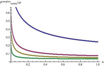
We can fit the Hilbert-Schmidt curve here very well–the integral over of the sum of squares of the differences being only 0.00030092–while achieving our conjectured separability probability of [7] with the function
| (7) |
where . Also, the square of the real counterpart (6) does provide a close fit to the Hilbert-Schmidt curve in Fig. 2. (However, our conjectured complex two-qubit separability probability of is not equal to the square, , of the conjectured real separability probability of , so conformity to a Dyson-index pattern is not total.)
Additionally, we can very well fit the Bures curve in Fig. 2 and our corresponding conjectured ”silver mean” separability probability (2) [4] by the function (of the seventh root of )
| (8) |
(The sum-of-squares measure of fit between the two curves is 0.000739208. However, the [exact] square root of (8)–deviating substantially from a Dyson-index-like pattern–does not at all provide a close fit [as in the HS case] to the real Bures counterpart in Fig. 1.)
II.2 Second set of constraints–convex combinations of minimum eigenvalues of and
II.2.1 Real two-qubit density matrices
In Fig. 3 we show as a function of , the probabilities for a generic (9-dimensional) real two-qubit system that
| (9) |
where the subscript denotes the smallest of the corresponding four eigenvalues () of either or . (As noted, having all eigenvalues nonnegative is fully equivalent to having a nonnegative determinant for the partial transpose of a density matrix [34]. The entanglement measure negativity is equal to [16, p. 401]. The Hilbert-Schmidt distance of an entangled state to the set of all partially transposed sets can be expressed as a function of the negative eigenvalues of the partial transpose of the entangled state [35].)
II.2.2 Complex two-qubit density matrices
In Fig. 4 we show as a function of , the probabilities for a generic (15-dimensional) complex two-qubit system that the inequality constraint (9) holds.


One can fit the complex HS curve rather closely by the square of the corresponding real HS curve, particularly so if one adds a small linearly increasing correction of the form to this square.
II.3 Third set of constraints–determinants of convex combinations of and
II.3.1 Real two-qubit density matrices
In Fig. 5 we show as a function of , the probabilities for a generic (9-dimensional) real two-qubit system that the positive ”twofold partial” transpose condition,
| (10) |
holds. The Hilbert-Schmidt curve is highly linear in character. The line closely approximates it, as well as reproducing the conjectured separability probability of .
II.3.2 Complex two-qubit density matrices
In Fig. 6 we show as a function of , the four probabilities () for a generic complex two-qubit system that the inequality (9) holds.
In computing Figs. 5 and 6, we solve the quartic equation and assume that there can not be more than one solution . (Numerically, this did appear to be the case, except for some isolated instances in which two positive [essentially identical] roots both very close to zero were found.)
Another possible generalized Peres-Horodecki condition–that is, that the minimum eigenvalue of be nonnegative–appeared to be considerably more problematical (time-consuming) than (10) to investigate, though we do, in fact, implement such a condition for the generic complex qubit-qutrit systems (sec. IV) and in generating Fig. 14.
Let us note that all the curves displayed so far in this communication appear to correspond to convex functions, but for the last two Hilbert-Schmidt curves.


II.4 Comparison of metric-specific curves for the first three sets of constraints
In Fig. 7 we show in a single plot, the three Hilbert-Schmidt curves plotted above (one per figure) for the generic real 9-dimensional two-qubit systems, while in Fig. 8 we show in a single plot, the three Bures curves plotted above for the generic complex 15-dimensional two-qubit systems. In both these figures the order of dominance of the curves is the same–the curve based on the constraint (10) dominates that based on (9), which, in turn, dominates that based on (4).


Of course, we find in both of these figures that the three curves have common points-of-intersection at , corresponding to the ”ordinary” separability probability (as well as ).
III Generic rank-3 complex two-qubit case
The ”twofold” volume-to-area-ratio theorem of Szarek, Bengtsson and Życzkowski [36] allows us to immediately extend our conjecture [7] of Hilbert-Schmidt separability probability of for the 15-dimensional generic complex two-qubit states to the fully equivalent conjecture that the HS separability probability of the states on the 14-dimensional boundary is one-half of this, that is, . In Figs. 9 and 10 we show our corresponding estimation of the -separabilities based on certain obvious modifications of the determinant constraint (4) and the minimum eigenvalue constraint (9). That is, rather than using the (zero) determinant of the rank-three density matrix, we use its generically nonzero principal minor. Further, rather than using the minimum (zero) eigenvalue, we employ the minimum of the generically three nonnegative eigenvalues.


In Fig. 11 we display the rank-3 -separability probability estimates based on the application of the constraint (10). Here we notice some unusual behavior near due to the degeneracy (zero determinant) of a rank-3 two-qubit () density matrix.

IV Generic full-rank complex qubit-qutrit case
Of the three distinct sets of constraints considered in the two-qubit case, only (9) seemed immediately adoptable to the qubit-qutrit case associated with density matrices. In our computations, we now employ the associated Euler-angle parameterization [21, sec XI]. In Fig. 12 we show the corresponding plot.
Further, by specifically checking nonnegativity at each value of , we were able to enforce the condition that the minimum eigenvalue of the matrix convex combination be nonnegative. (Nonnegativity of the determinant of the partial transpose is no longer equivalent–as it is in the two-qubit case [34]–to having no negative eigenvalues, since two negative eigenvalues yields a positive determinant.) The corresponding plot is displayed in Fig. 13.


We can ”sandwich” the Hilbert-Schmidt curve in Fig. 12 between two curves, corresponding to exact squares, both of which yield the conjectured separability probability of . These functions are
| (11) |
V Extending range of -parameter
We have, so far, considered our primary variable as extending over the unit interval [0,1]. However, it appears quite interesting and possibly more natural to formally view its range as the real line . In a further analysis, we developed a plot (Fig. 14) over , of the estimated -probability that the matrix , where is a generic complex two-qubit density matrix, has all its four eigenvalues nonnegative.

VI Concurrence-related analyses
VI.1 Generalized Peres-Horodecki conditions
In all the analyses reported above, the nonnegativity convex combination constraints (”generalized Peres-Horodecki conditions”) utilized, have been expressed either in terms of the determinant or the minimum eigenvalue of . In the two-qubit case, we have also been able to investigate similiarly-motivated conditions using, in conjunction, the maximal concurrence over spectral orbits (1) [24] of a two-qubit density matrix (), and its concurrence [22]
| (12) |
(Here, the ’s are the ordered eigenvalues of and the ’s are the ordered eigenvalues of , where , and is a Pauli matrix, and denotes conjugation. Throughout the reminder of the paper, the symbol –consistently with our previous notation–will denote a ”separability function, and not a Pauli matrix.) The corresponding constraint we employ is
| (13) |
Since , the constraint holds trivially for . In Figs. 15 and 16, we show for the half-interval , the curves for the generic real and complex two-qubit states, respectively, based on (13), while in Figs. 17 and 18, we display the corresponding plots for the generic rank-3 real and complex two-qubit states, respectively.


VI.2 Separability probabilities as functions of concurrence–intersecting curves
In this section, we depart from the basic paradigm so far employed in first basic part (”generalized Peres-Horodecki conditions”) of the paper, in which we use convex combinations of quantum-mechanical terms to form nonnegativity constraints.
Now, we simply estimate–again, with respect to the four metrics in question–the separability probability of two-qubit states for which the concurrence is less than some threshold . We show our results in Figs. 19 and 20.


In all four of these cases, the Hilbert-Schmidt curve intersects the curves for the three monotone metrics from below. In this regard, it has been noted by Bengtsson and Życzkowski that the ”Bures measure is concentrated at the states of higher [than the Hilbert-Schmidt] purity” [16, p. 356], since . Our (intersecting) results in this set of concurrence-based analyses is clearly consistent–but now taking a separability-related form–with that assertion.
VII Remarks
Our motivation in undertaking the first principal part of this study reported above has been to examine whether it might be feasible to shift the question of determining the two-qubit separability probabilities with respect to various metrics of quantum-mechanical interest to the (perhaps more tangible, addressable) question of characterizing the curves that interpolate between such separability probabilities and the (unit) probabilities that a two-qubit state is either separable or entangled (cf. [13, 14]). We intend to study the curves generated in still greater detail, as additional computations render them more precise. (The Tezuka-Faure procedure is not amenable to use of statistical tests, though variants of this quasi-Monte Carlo method have been developed that are.) In particular, it would be of interest to see if the differences between the curves for the three monotone metrics studied could be explained directly in terms of the Chentsov-Morozova functions for those metrics [26, 37]. These are , and , for the Bures, Wigner-Yanase and Kubo-Mori metrics, respectively. (The associated operator monotone functions, , for which are , and , respectively.) The possible relevance of the Dyson-index-ansatz to explain differences between results for the generic real and generic complex systems–as in sec. VIII below–should also be examined [7, 17].
Conceiveably, our attempted generalizations here of the Peres-Horodecki conditions and introduction of the concept of ”-separability” might prove productive in some manner parallel to the well-studied concepts (also based on generalizations/extensions/embeddings) of -Rényi-entropy [38] and of escort distributions [39, 40].
VIII Separabilities as piecewise continuous functions of maximal concurrence
VIII.1 Objective
Here, we begin the second basic part of our paper. We importantly amend a certain parenthetical remark made in our recent paper [17], to the effect that although two-qubit diagonal-entry-parameterized separability functions (DESFs) had been shown [7, 31] to clearly conform to a pattern dictated by the “Dyson indices” ( [real], 2 [complex], 4 [quaternionic]) of random matrix theory, this did not appear to be the case with regard to eigenvalue-parameterized separability functions (ESFs). (We remark here that the ”value of is given by the number of independent degrees of freedom per matrix element and is determined by the antiunitary symmetries …It is a concept that originated in Random Matrix Theory and is important for the Cartan classification of symmetric spaces” [41, p. 480]. The Dyson index corresponds to the “multiplicity of ordinary roots”, in the terminology of symmetric spaces [42, Table 2].) But upon further examination of the extensive numerical analyses reported in [17], we found quite convincing evidence that adherence to the Dyson-index pattern does also hold for ESFs, at least as regards the upper half-range of the maximal concurrence over spectral orbits (1).
To be specific, it strongly appears that in this upper half-range, the real two-qubit ESF is equal to to , and its complex counterpart–in conformity to the Dyson-index pattern–proportional to the square of the real ESF, that is, . The previously documented piecewise continuous (“semilinear”) behavior in the lower half-range appeared to lack any particular Dyson-index-related interpretation–which seemed somewhat paradoxical in terms of our DESF-findings [7, 31]. However, we report new insights into this problem below (sec. IX.3).
VIII.2 Previous ESF findings
The study [17] had been devoted to the question of determining for the generic (9-dimensional) real and (15-dimensional) complex two-qubit systems, the nature of certain trivariate “eigenvalue-parameterized separability functions” (ESFs). These (metric-independent) ESFs, it was argued, could substantially assist in the determination of separability probabilities in terms of certain metrics (the Hilbert-Schmidt and Bures being the most conspicuous examples). (In [7], DESFs were successfully used in the Hilbert-Schmidt case, but they do not seem as useful for the Bures and other montone metrics, the standard formulas for which are expressed in terms of eigenvalues, and not diagonal entries.) We further investigated in [17] the possibility that these prima facie trivariate functions of the eigenvalues of density matrices , were expressible as univariate functions
| (14) |
of the maximal concurrence –given by (1)–over spectral orbits [24, sec. VII] [43, 44]. (At this point in our presentation, let us–motivated by Dyson-index conventions–regard in (14) only as a notational [dummy variable], not calculational device taking the values 1 [real], 2 [complex], 4 [quaternionic].)
VIII.3 Jump discontinuities
Our main conclusions in [17] were that–if the reducibility-to-univariance property (14) held, as our extensive numerical evidence appeared to suggest might be the case (being able to explain almost of the variance [17, Sec. II.B.1])–the associated real and complex univariate functions both had jumps of approximately magnitude at , as well as a number of additional discontinuities (remarkably coincident in both the real and complex cases) in the lower half-range . (The joint jumps at were displayed in [17] in Figs. 2 and 6. We have since found a small programming error that caused the two curves in Fig. 2 there to be slightly more misaligned–by –than they should have been.) Also, both univariate functions appeared to be simply linear between certain of these discontinuities. The upper half-range –in which the univariate functions of took lesser values–did not command our attention in [17], seeming to be of relatively less interest. Our only pertinent observation there was that there did not appear to be any discontinuities in that segment.
VIII.4 New Dyson-index-related findings
Now, in fact, turning our attention more closely to this upper half-range , we readily find strong evidence for a very interesting Dyson-index-type phenomenon. If we normalize our extensive numerical estimates from [17] of and to both equal 1 at the jump discontinuity point , then a joint plot (Fig. 23) of the latter normalized (complex) function versus the square of the former normalized (real) function for remarkably shows no perceptible difference between the two resulting curves. (The sample [quasi-Monte Carlo] estimate of is 0.0651586 and that of is 0.1803748.)
In Fig. 24, we show–on a much finer scale than used in Fig. 23–the actual (very small) numerically-obtained differences
| (15) |
between them.
Of further considerable importance, Fig. 25 is a repetition of Fig. 23, but along with the insertion now of the function
| (16) |
which we see fits our two estimates very well.
Assuming that (16) is the correct form (up to the still not exactly-known normalization factor) of over , we can estimate the associated contribution to the separability probabilities from density matrices corresponding to this half-range to the Hilbert-Schmidt and Bures separability probabilities of generic complex two-qubit systems to be 0.0100578 and 0.0194829, respectively. (The real counterparts of these separability probabilities are, then, 0.0254346 and 0.0100578, respectively [cf. (29), (30)].)
Let us further note that our sample estimate of the ratio
| (17) |
is very close (and possibly theoretically exactly equal) to 2.
Over , the range of primary interest in [17], the estimates of the real and complex two-qubit separability functions intersect (near ), and appear to have linear segments over the same subintervals [17, Figs. 1, 5, 7]. These features appeared to make any immediate application of the Dyson-index pattern problematical in this lower half-range. So, the behaviors of the univariate functions , ( [real], 2 [complex]), over the two indicated regimes of seem to be highly distinct. The point clearly serves as a point of major behavioral transition, with the lower half-range, then, appearing perhaps to be the more theoretically challenging of the two. (We will observe what appears to be similarly dichotomous Dyson-index behavior in the qubit-qutrit case [Fig. 31]. Perhaps one might view the two regimes as semiclassical and quantum in nature.)
An outstanding question is what are the specific values of and , which we used as normalization factors in our analyses above. The nearness to 2 of the ratio (17) may be a helpful guide in this regard. In fact, let us take this opportunity to further indicate that in our ongoing supplemental analyses–in which we use 5,000, rather than 500 sampling points in the interval [0,1]–we have obtained for the ratio (17) the estimate
| (18) |
This ratio would be exactly 2 if we took for the numerator of (18) the value and for the denominator, . We will, in fact, assume these exact values in seeking to ascertain in sec. IX, the exact contributions over to the total Hilbert-Schmidt two-qubit generic real and complex separability probabilities.
VIII.5 Rank-three complex and real two-qubit cases
Here, we straightforwardly apply the same maximal-concurrence ansatz (14) just discussed and applied to the full (rank-4) complex and real two-qubit cases, to the minimally degenerate (rank-3) counterparts. The main conceptual point to note is that the formula for the maximal concurrence (1) now degenerates to
| (19) |
In Fig. 26 we show the joint plot of the corresponding real and complex curves. The estimated complex (red) curve initially dominates the estimated real (blue) curve (cf. [17, Fig. 1]).

VIII.5.1 Close resemblance to generic rank-4 Dyson-index pattern
It appears now–as a plot (Fig. 27) parallel to that displayed in Fig. 25 indicates–that the Dyson-index pattern continues to hold for the range in the two-qubit generic rank-3 cases, but with the replacement of by .

To test the possible applicability of the rank-3 version of the univariance hypothesis (14), we estimated the real and complex rank-3 two-qubit Hilbert-Schmidt separability probabilities using the ESFs displayed in Fig. 26. The values we obtained were 0.208172 and 0.104852, respectively (while the correponding conjectured values were perhaps somewhat disappointingly different, calling for further analysis, that is and ). We can express these results as one-dimensional integrals over of the product of the real function displayed in Fig. 26, and (using ) the univariate marginal Hilbert-Schmidt probability distribution (Fig. 28)
| (20) |
and the integral over of the product of the complex function displayed in Fig. 26, and the univariate marginal Hilbert-Schmidt probability distribution (Fig. 28)
| (21) |
(These distributions are ”marginal”, in the sense that they are obtained by integrating the HS or Bures measure defined on the three-dimensional simplex of eigenvalues–obtainable from the papers of Życzkowski and Sommers [13, 14]–over two of the three coordinates [the third coordinate being ] used to parameterize the simplex.) Also, we have for ,
| (22) |
(The quaternionic expression for is somewhat more cumbersome in nature to present.) To obtain these univariate functions, we have transformed one of the eigenvalues, say to (the jacobian of the transformation being unity) and integrated (restricted to the Weyl chamber of ordered eigenvalues) the corresponding (bivariate in this case) Hilbert-Schmidt measures (over the eigenvalues) [13, eqs. (4.1), (6.5), (7.8)] over . Fitting the means and variances of ((20)-(22)), we can obtain beta distribution approximations to the real, complex and quaternionic probability distributions using the paired sets of parameters and , respectively. Beta distributions, defined over the unit interval, are a general type of statistical distribution, related to the gamma distribution, and have two free parameters.
The Hilbert-Schmidt (total–separable and nonseparable) probability that a minimally-degenerate two-qubit state has maximal concurrence within the range is for real states, for complex states, and for quaternionic states. (For the [smaller] full-rank counterparts see sec. IX.4.)


Let us assume (cf. Fig. 27) that the ESF in the real case is proportional over to and in the complex case to the square of this. Then, we have that the contributions over this half-domain to the Hilbert-Schmidt real and complex separability probabilities, respectively, are (multiplied by a normalization constant approximately 0.177365) and (multiplied by a normalization constant approximately 0.086232).
VIII.6 Rank-five complex qubit-qutrit case
For the full-rank qubit-qutrit case, the counterpart–although not enjoying all the properties–of the two-qubit maximal concurrence formula (1) is [24, p. 16]
| (23) |
which, obviously (since ), degenerates (using the same eigenvalue-ordering) to
| (24) |
In Fig. 30–again under the hypothesis (ansatz) that the corresponding eigenvalue-parameterized-separability function is a (univariate) function of the maximal concurrence expression (24)–we show the analogue of Fig. 26 for the minimally-degenerate (rank-5) generic real and complex qubit-qutrit case. (Again, in the complex case we used the -Euler-angle parameterization of S. Cacciatori [8, App. A], while we used a yet unpublished Euler-angle parameterization of his of for the real case.) There are evident jumps in the real (blue) curve at and . (The still erratic nature of the complex [red] curve–we used 1,000 [not 500] equally-spaced points in [0,1]–makes it, at this point of sampling, difficult to gauge the applicability of the Dyson indices.)

To test the applicability of the rank-5 version of the univariance hypothesis (14), we estimated the real and complex rank-5 qubit-qutrit Hilbert-Schmidt separability probabilities using the ESFs displayed in Fig. 30. The values we obtained were 0.097232 and 0.0226654, respectively, while the corresponding conjectures were–again somewhat disappointingly different– and .
VIII.7 Full-rank real and complex qubit-qutrit cases
In the two-qubit case, we had evolved a computational strategy in which we used the Mathematica command FindInstance to systematically generate random sets of three or four eigenvalues that yielded values of the maximal concurrence ((1) or (19)) at equally-spaced intervals –and, similarly, in the rank-5 qubit-qutrit case (24). However, due to greater complexity in the rank-6 case, this strategy did not prove at all feasible for generating random sets of six eigenvalues yielding equally-spaced values of the maximal concurrence (23).
So, we altered our approach, now simply randomly generating density matrices (again using the same quasi-Monte Carlo routines [20]) and recording their associated values of concurrence. We ”binned” these concurrence values into intervals of length , and averaged the total measures recorded by the number of observations within the individual bins. We interpolated these average values to obtain the associated eigenvalue-parameterized separability functions (ESFs). We have generated the corresponding curves for both the full-rank real and complex generic qubit-qutrit cases, but they are still somewhat crude/rough in character. Nevertheless, we plot in Fig. 31 (cf. Figs. 23 and 27) normalized forms of the complex (red) curve and the square of the real (blue) curve. They appear to indicate possible adherence to the Dyson-index ansatz, since the two curves closely ”track” each other, at least (as our generally observed pattern in the two-qubit case would suggest) for the higher values of . (It seems that this domain of possibly strict Dyson-index behavior may be , while in the full-rank two-qubit case (Fig. 23) it highly convincingly appeared to be . Our level of binning is perhaps too coarse for the detection of possible discontinuities in the two curves.)

We were interested in seeing how close the plotted curves came–under the rank-6 qubit-qutrit version of the univariance hypothesis (14)–to yielding the conjectured HS real and complex separability probabilities of and [7, sec. X], but the requisite numerical integrations proved quite problematical to perform. In Fig. 32 we plot the two functions in Fig. 31 over the interval , along with the interweaving curve .

.
IX Separability probability decompositions over regions
IX.1 domain
One can–in an apparently natural manner–consider the two-qubit real, complex and quaternionic Hilbert-Schmidt separability probabilities to be the sum of three components: (1) the Hilbert-Schmidt absolute separability probabilities (corresponding to ); (2) the probabilities over the range ; and (3) the probabilities over the range . (For a contour plot of the three-dimensional body , see [8, Fig. 2].) Now, we have previously been able to compute the absolutely separable components [8, eqs. (34), (35)]. These are
| (25) |
| (26) |
(the Bures [minimal monotone] metric analogue being considerably smaller, 0.000161792 [8, p. 25]) where
and
| (27) |
where
| (28) |
(These are ”conjecture-free” results, not dependent on any Dyson-index ansatz. In [8, eqs. (36), (37)] we gave a considerably lengthier, but fully equivalent, expression for . One might seek to find explanations for the large integers displayed above in terms of gamma functions. The computational challenges to computing analogous absolute separability results for the qubit-qutrit states appear to be highly formidable.)
IX.2
Further, accepting the strongly-supported Dyson-index ansatz (Fig. 25 and (18)) that and for , we can now add to the absolute separability probabilities () listed immediately above, the conjectured probability contributions
| (29) |
and
| (30) |
Further, using the Dyson-index ansatz with , we obtain
| (31) |
where
| (32) |
and is the unknown and yet-unconjectured analogue of the presumed real and complex constants and . (In computing (29)-(32), we found a joint transformation of the form and to be helpful.)
IX.2.1 Corollaries to the ”twofold” SBZ-Theorem
Since the probability is zero that a generic minimally-degenerate two-qubit state is absolutely separable (that is, )–as can be immediately deduced from (24)–we have simple corollaries to the twofold-theorem of Szarek, Bengtsson and Życzkowski [36] of the form
| (33) |
where the ’s are Hilbert-Schmidt separability probabilities, for the real, complex or quaternionic two-qubit states.
IX.3
So, the most conspicuous missing parts in the Hilbert-Schmidt separability probability ”puzzle” appear to us to be formulas for and . Of course, we can subtract the sums of the other two parts (, and ) from our overall conjectures of and to obtain ”induced” conjectures about these third components.
Since it now appears crucial to, additionally, model the eigenvalue-parameterized separability functions over the domain , we present in Fig. 33, for the convenience of the interested reader, the previously-generated [17, Fig. 1] estimates of these functions. The real (blue) curve is close to linear (). Also, we have noted that the complex (red) curve is quite well-fitted by and . However, we appear here to lack a strictly similar Dyson-index ansatz to serve as a guide in constructing these two functions (cf. [7]). Also, there were indications given in [17, Figs. 3-5] that these two functions have multiple (matching) points of discontinuity in . (These were .)

The lack of a Dyson-index pattern strictly similar to that found apparently for to exploit for is immediately apparent from Fig. 34. A flat line over at least some subdomain of would indicate such a Dyson-index pattern. Clearly, no such flatness appears there. However, it now seems that there is a pattern of the approximate form
| (34) |
(We have already noted that in this half-domain.) The highly interesting nature of Fig. 34 led us to similarly re-examine the minimally degenerate rank-3 two-qubit scenarios (Fig. 26). Thus, we obtained Fig. 35. Now serves as an excellent linear approximation, and we have a relation analogous to (34)
| (35) |


If we plot vs. and also vs. over the half-domain, the two curves within each set are essentially indistinguishable. We have investigated analogous plots of the same form for the minimally-degenerate qubit-qutrit (Fig. 30) and full-rank (Fig. 31) cases over . They are much rougher in nature, due to our limited sampling, but still indicate initial monotonically-increasing (non-flat) behavior over .
IX.4 Total probabilities over regions
Let us also point out that the Hilbert-Schmidt probability () that a generic two-qubit real state (separable or entangled) lies in the domain is
| (36) |
with the complex counterpart being
| (37) |
and the quaternionic analogue being
| (38) |
where
| (39) |
(The comparable total probabilities for the minimally-degenerate two-qubit states have been given in sec. VIII.5.1.) Since for the absolutely separable states (), the two probabilities and are equivalent, we can immediately determine (by subtracting from 1 our known HS probabilities and ) the complementary probabilities, . Numerically, these are and .
X Concluding remarks
Our analyses of two-qubit diagonal-entry-parameterized separability functions (DESFs) [45, 7, 31] and eigenvalue-parameterized separability functions (ESFs) [8, 17] completely share a common goal: the determination of two-qubit separability volumes and probabilities (in terms of various metrics). As pieces of these formidable objectives begin to be assembled, we can pose a further challenge–to find transformations between the two different sets of coordinates used–that is, (1) the diagonal entries and (2) the eigenvalues of density matrices–that will map one set of separability functions into the other. The Schur-Horn Theorem, which asserts that the decreasingly-ordered vector of eigenvalues of an Hermitian matrix majorizes the decreasingly-ordered vector of its diagonal entries [46, chap. 4] (cf. [47, 48]), would appear to be of possible relevance in this regard, particularly since the maximal concurrence over spectral orbits (12) is expressed in terms of the ordered eigenvalues.
In terms of the diagonal entries () of two-qubit density matrices, we can express the conjectured Hilbert-Schmidt separability probability [7], , of generic complex states in the form
| (40) |
where , and the integration extends over the unit simplex, but with the restriction . (We note that . Let us also observe that the variable conveniently ranges over the entire real axis and is symmetric about the origin.)
Additionally, in terms of the eigenvalues () of two-qubit density matrices, we can express this same separability probability as (cf. (14))
| (41) |
and the integration extends over that part (Weyl chamber [16]) of the unit simplex for which . (We note that, interestingly, in light of the just previous factorization, .) Here is the (two-qubit complex []) eigenvalue-parameterized separability function that we have previously sought to determine [17, Fig. 1], and was found to be very well-fitted by for (Fig. 25 and (18)). (It is possible to reexpress these two last integrals so that both are taken over the same complete 3-dimensional unit simplex.) Further still, our generic complex two-qubit Bures separability probability conjecture (2) [4, Table VI] takes the form
| (42) |
It is abundantly clear: (a) that this (piecewise continuous) function has a jump discontinuity at (as well as does its real counterpart ; and (b) that in the diagonal-entry-parameterized scenario, the value is a locus of special symmetry. In this regard, we might speculate that if one can find a coordinate transformation between the two separability probability expressions ((40) and (41)), then those values of the ’s for which will be mapped to those values of the ’s for which .
Through the use of the jacobian transformation of the diagonal entry (say) to [45, eq. (11)], and subsequent integration over and , it is possible to explicitly reduce the computation of the trivariate integral (40) to that of a univariate integral in . In Fig. 36, we show–based on numerical calculations–the univariate marginal probability distributions of the Hilbert-Schmidt measure over the real and complex two-qubit states in terms of (cf. (20)-(22)). Similarly to their rank-3 counterparts( Fig. 28), these curves have differently-positioned peaks, and are not symmetric, but skewed to the right. (We take the range of to be , to accord with actual values, rather than the conventional [cf. (12)].) In Fig. 37, we show the Bures-metric counterpart, although we encounter some ”glitch” in displaying the real curve here.


The counterparts to the formulas (40) and (41), in light of our conjecture [7] that the Hilbert-Schmidt separability probability of the generic real two-qubit states is , are (the domains of integration being the same)
| (43) |
and
| (44) |
(Here, and . It appears [Fig. 27 and (18)) that possibly for .)
Let us point out the possible relevance of the concept of the Thouless energy [49, p. 734] in the modeling of the threshold or crossover effect we have numerically observed for eigenvalue-parameterized separability functions in both the full generic real and complex two-qubit and qubit-qutrit cases. There, the Dyson indices () of random matrix theory only seemed to apply above a certain value of the maximal concurrence (that is, in the two-qubit case, and possibly in the qubit-qutrit instance). (It remains to formally reconcile these observations with the ones that, in terms of diagonal-entry-parameterized separability functions, Dyson-index behavior appear to be strictly followed [7].)
Acknowledgements.
I would like to express appreciation to the Kavli Institute for Theoretical Physics (KITP) for computational support in this research, as well as to K. Życzkowski for his interest and for a number of suggestions concerning the analyses and their presentation.References
- [1] K. Życzkowski, P. Horodecki, A. Sanpera, and M. Lewenstein, Phys. Rev. A 58, 883 (1998).
- [2] P. B. Slater, J. Phys. A 32, 5261 (1999).
- [3] P. B. Slater, Euro. Phys. J. B 17, 471 (2000).
- [4] P. B. Slater, J. Geom. Phys. 53, 74 (2005a).
- [5] P. B. Slater, Phys. Rev. A 71, 052319 (2005b).
- [6] P. B. Slater, J. Phys. A 39, 913 (2006a).
- [7] P. B. Slater, J. Phys. A 40, 14279 (2007a).
- [8] P. B. Slater, J. Geom. Phys. 59, 17 (2009).
- [9] L. M. Ioannou, Quant. Inform. Comput. 7, 335 (2007).
- [10] D. Ye, eprint arXiv:0902.1505.
- [11] K. Appel and W. Haken, Ill. J. Math. 21, 439 (1977).
- [12] A. Soifer, The mathematical coloring book (Springer, New York, 2009).
- [13] K. Życzkowski and H.-J. Sommers, J. Phys. A 36, 10115 (2003).
- [14] H.-J. Sommers and K. Życzkowski, J. Phys. A 36, 10083 (2003).
- [15] A. Andai, J. Phys. A 39, 13641 (2006).
- [16] I. Bengtsson and K. Życzkowski, Geometry of Quantum States (Cambridge, Cambridge, 2006).
- [17] P. B. Slater, J. Phys. A 41, 505303 (2008a).
- [18] T. Tilma, M. Byrd, and E. C. G. Sudarshan, J. Phys. A 35, 10445 (2002).
- [19] H. Faure and S. Tezuka, in Monte Carlo and Quasi-Monte Carlo Methods 2000 (Hong Kong), edited by K. T. Tang, F. J. Hickernell, and H. Niederreiter (Springer, Berlin, 2002), p. 242.
- [20] G. Ökten, MATHEMATICA in Educ. Res. 8, 52 (1999).
- [21] T. Tilma and E. C. G. Sudarshan, J. Phys. A 35, 10467 (2002).
- [22] W. K. Wootters, Phys. Rev. Lett. 80, 2245 (1998).
- [23] T. Iwai, J. Phys. A 40, 1361 (2007).
- [24] R. Hildebrand, J. Math. Phys. 48, 102108 (2007).
- [25] M. Ozawa, Phys. Lett. A 268, 158 (2000).
- [26] D. Petz and C. Sudár, J. Math. Phys. 37, 2662 (1996).
- [27] P. Gibilisco and T. Isola, J. Math. Phys. 44, 3752 (2003).
- [28] D. Petz, J. Math. Phys. 35, 780 (1994).
- [29] C. Krattenthaler and P. B. Slater, IEEE Trans. Info. Theory 46, 801 (2000).
- [30] M. Hayashi, eprint arXiv:0806.1091.
- [31] P. B. Slater, J. Geom. Phys. 58, 1101 (2008b).
- [32] A. Peres, Phys. Rev. Lett. 77, 1413 (1996).
- [33] M. Horodecki, P. Horodecki, and R. Horodecki, Phys. Lett. A 223, 1 (1996).
- [34] R. Augusiak, R. Horodecki, and M. Demianowicz, Phys. Rev. 77, 030301(R) (2008).
- [35] F. Verstraete, J. Dehaene, and B. D. Moor, J. Mod. Opt. 49, 1277 (2002).
- [36] S. Szarek, I. Bengtsson, and K. Życzkowski, J. Phys. A 39, L119 (2006).
- [37] A. Lesniewski and M. B. Ruskai, J. Math. Phys. 40, 5702 (1999).
- [38] R. Alicki and M. Fannes, Open Syst. Inform. Dyn. 11, 339 (2004).
- [39] S. Abe, Phys. Rev. E 68, 031101 (2003).
- [40] P. B. Slater, J. Math. Phys. 47, 022104 (2006b).
- [41] J. B. Kogut, M. A. Stephanov, D.Toublan, J. J. M. Verbaarschot, and A. Zhitnitsky, Nucl. Phys. B 582, 477 (2000).
- [42] M. Caselle and U. Magnea, Phys. Rep. 394, 41 (2004).
- [43] S. Ishizaka and T. Hiroshima, Phys. Rev. A 62, 022310 (2000).
- [44] F. Verstraete, K. Audenaert, and B. DeMoor, Phys. Rev. A 64, 012316 (2001).
- [45] P. B. Slater, Phys. Rev. A 75, 032326 (2007b).
- [46] R. A. Horn and C. R. Johnson, Matrix Analysis (Cambridge Univ., New York, 1991).
- [47] M. A. Nielsen and G. Vidal, Quant. Inform. Comput. 1, 76 (2001).
- [48] E. A. Carlen, eprint math.FA/0904.0734.
- [49] C. W. J. Beenakker, Rev. Mod. Phys. 69, 731 (1997).