The one-loop pentagon to higher orders in $\epsilon$Preprint: IPPP/09/25
CP3-09-15

In the planar $\cal N=4$ supersymmetric Yang-Mills theory, Anastasiou, Bern, Dixon and Kosower (ABDK) [2] proposed an iterative structure for the colour-stripped two-loop scattering amplitude with an arbitrary number $n$ of external legs in a maximally-helicity violating (MHV) configuration. The proposed iteration formula for the two-loop MHV amplitude $m_{n}^{(2)}(\epsilon)$ is

$$m_{n}^{(2)}(\epsilon)=\frac{1}{2}\left[m_{n}^{(1)}(\epsilon)\right]^{2}+f^{(2)}(\epsilon)\,m_{n}^{(1)}(2\epsilon)+C^{(2)}+\cal O(\epsilon)\,,$$

(1)

thus the two-loop amplitude is determined in terms of the one-loop MHV amplitude $m_{n}^{(1)}(\epsilon)$ evaluated through to $\cal O(\epsilon^{2})$ in the dimensional-regularisation parameter $\epsilon$, a constant, $C^{(2)}$, and a function, $f^{(2)}(\epsilon)$, which is related to the cusp [3, 4] and collinear [5, 6] anomalous dimensions.

Subsequently, Bern, Dixon and Smirnov (BDS) proposed an all-loop resummation formula [7] for the colour-stripped $n$-point MHV amplitude, which implies a tower of iteration formulæ, allowing one to determine the $n$-point amplitude at a given number of loops in terms of amplitudes with fewer loops, evaluated to higher orders of $\epsilon$. BDS checked that the ansatz was correct for the three-loop four-point amplitude, by evaluating analytically $m_{4}^{(3)}(\epsilon)$ through to finite terms, as well as $m_{4}^{(2)}(\epsilon)$ through to $\cal O(\epsilon^{2})$ and $m_{4}^{(1)}(\epsilon)$ through to $\cal O(\epsilon^{4})$. The BDS ansatz has been proven to be correct also for the two-loop five-point amplitude [8, 9], for which $m_{5}^{(2)}(\epsilon)$ has been computed numerically through to finite terms, as well as $m_{5}^{(1)}(\epsilon)$ through to $\cal O(\epsilon^{2})$.

In the strong-coupling limit, Alday and Maldacena showed that the ansatz is violated for amplitudes with six or more legs [10]. This provoked the numerical calculation of $m_{6}^{(2)}(\epsilon)$ through to finite terms and of $m_{6}^{(1)}(\epsilon)$ through to $\cal O(\epsilon^{2})$, where the BDS ansatz was demonstrated to fail in Ref. [11], and where it was shown that the finite pieces of the parity-even part of $m_{6}^{(2)}(\epsilon)$ are incorrectly determined by the ansatz¹¹ 1 It was subsequently shown that the parity-odd part of $m_{6}^{(2)}(\epsilon)$ does satisfy the ansatz [12].. In particular, it was shown that the remainder function,

$$R_{n}^{(2)}=m_{n}^{(2)}(\epsilon)-\frac{1}{2}\left[m_{n}^{(1)}(\epsilon)\right]^{2}-f^{(2)}(\epsilon)\,m_{n}^{(1)}(2\epsilon)-C^{(2)}\,,$$

(2)

is different from zero for $n=6$, where $R_{n}^{(2)}$ may be a function of the kinematical parameters of the $n$-point amplitude, but a constant with respect to $\epsilon$. Because the calculation of Ref. [11] is numerical, the analytic form of $R_{6}^{(2)}$ is unknown.

Using the AdS/CFT correspondence, Alday and Maldacena [13] showed that in the strong-coupling limit planar scattering amplitudes exponentiate like in the BDS ansatz, and suggested that in the weak-coupling regime the vacuum expectation value of the $n$-edged Wilson loop could be related to the $n$-point MHV amplitude in $\cal N=4$ super Yang-Mills theory. The agreement (up to a constant) between the light-like Wilson loop and the (parity-even part of the) MHV amplitude has been verified for the one-loop four-edged [14] and $n$-edged [15] Wilson loops, and for the two-loop four-edged [16], five-edged [17] and six-edged [18, 19] Wilson loops. Furthermore, it was shown that the light-like Wilson loop exhibits a conformal symmetry, and that the BDS ansatz is a solution of the ensuing Ward identities, up to functions of conformally invariant cross-ratios, which are present for $n\geq 6$ [17]. Recently, also the two-loop seven-edged and eight-edged Wilson loops have been computed numerically [20], although no corresponding $\cal N=4$ MHV amplitudes are known. Thus, also the remainder functions $R_{7}^{(2)}$ and $R_{8}^{(2)}$ (for the Wilson loops, as well as for the MHV amplitudes, if we suppose that the agreement between them and the Wilson loops holds for seven or more points) are known numerically, and the numerical evidence [20] seems to confirm that they are functions of conformally invariant cross-ratios only. However, their analytic form is unknown.

Through to finite terms, one-loop $\cal N=4$ MHV amplitudes, $m_{n}^{(1)}(\epsilon)$, are parity-even and can be expressed in terms of box functions, which are massless for $n=4$, one-mass for $n=5$ and two-mass easy box functions for $n\geq 6$ [21]. For $n\geq 5$, parity-odd contributions and one-loop $n$-edged polygons occur in the higher orders in $\epsilon$ [22]. For example, an irreducible massless pentagon occurs in the parity-odd part of the one-loop five-point amplitude, which to all orders in $\epsilon$ is [8]

$$m_{5}^{(1)}=-\frac{1}{4}\sum_{\rm cyclic}s_{12}s_{23}I_{4}^{1m}(1,2,3,45,\epsilon)-\frac{\epsilon}{2}\epsilon_{1234}I_{5}^{6-2\epsilon}(\epsilon)\,,$$

(3)

where $m_{5}^{(1)}$ denotes the one-loop coefficient, i.e., the one-loop amplitude rescaled by the tree-level amplitude, and where the cyclicity is over $i=1,\ldots,5$, $I_{4}^{1m}(1,2,3,45,\epsilon)$ is the one-mass box with the massive leg of virtuality $s_{45}$, $I_{5}^{6-2\epsilon}(\epsilon)$ is a pentagon evaluated in $6-2\epsilon$ dimensions, and the parity-odd factor is $\epsilon_{1234}={\rm tr}[\gamma_{5}\!\!\not\!k_{1}\!\!\not\!\!k_{2}\!\not\!\!k_{3}\!\!\not\!k_{4}]$. A massless hexagon occurs in the parity-even part [11, 22], as well as a pentagon in the parity-odd part [12, 22], of the one-loop six-point amplitude at $\cal O(\epsilon)$. The hexagon may be reduced to one-mass pentagons. Thus, it seems fair to guess that the analytic form of the remainder function $R_{6}^{(2)}$ may be somewhat linked to the properties of the special functions occurring in the hexagon of the one-loop six-point amplitude.

Because very little is known in the literature about the analytic properties of pentagons and hexagons to higher orders in $\epsilon$, in this paper we perform a first study of the pentagon occurring in the parity-odd part of the one-loop five-point amplitude (3). A massless pentagon can in general be reduced to quadruple sums dependent on the four independent ratios of the kinematic invariants. In order to simplify matters, we choose a particular kinematic realm, the multi-Regge kinematics, where the quadruple sums reduce to double sums, which we proceed to study and expand to $\cal O(\epsilon^{2})$.

Our paper is organised as follows. As a prelude to our main objective which is the evaluation of the scalar massless pentagon integral in $D=6-2\epsilon$ dimensions in the multi-Regge limit, we first give a short review of multiple hypergeometric functions in Section 2. In general one may encounter a multiple hypergeometric function in several different representations - as a multiple sum, an Euler integral, a Mellin-Barnes representation or a Laplace integral. We then discuss in Section 3 different representations of Feynman integrals and show how they naturally match onto the various representations for hypergeometric functions. For example, in the Negative Dimension approach (NDIM) [23, 24] based on Schwinger parameters, one naturally finds the hypergeometric functions in the form of multiple sums. On the other hand, starting from Feynman parameters and utilising the Mellin-Barnes identity one naturally finds the hypergeometric functions as multiple Mellin-Barnes integrals. The one-loop pentagon integral and multi-Regge kinematics are defined in Section 4. In Euclidean kinematics, there are three distinct regions which we call I, II(a) and II(b). Regions II(a) and II(b) are related by symmetry. Regions I and II(a) are related by analytic continuation. We use two distinct methods to compute the massless pentagon integral in $D=6-2\epsilon$ dimensions in each of these regions and show (a) that the solutions in each region are the same for the two approaches and (b) that the solutions in region I and II(a) are related by analytic continuation. In Section 5, we use NDIM to write the integral as multiple hypergeometric sums. In the multi-Regge kinematics these sums collapse to hypergeometric sums of two variables. It is straightforward to make a Laurent expansion around $\epsilon=0$ and find that hypergeometric sums can be written in terms of transcendental double sums which we denote by ${\cal M}$ functions. In Section 6, we revisit the problem starting from the Mellin-Barnes representation of the pentagon integral. In the multi-Regge kinematics we obtain two Mellin-Barnes integrals. We show that by summing the residues, one recovers exactly the same hypergeometric sums as in NDIM. Alternatively, by performing the Mellin-Barnes integrals sequentially one can write the pentagon integral in terms of Goncharov’s polylogarithms. In Section 7 we perform the analytic continuation of the pentagon to the physical region where all $s$-type invariants are positive. Appendices with more details concerning the generalised hypergeometric functions, nested harmonic sums, ${\cal M}$ functions and Goncharov’s multiple polylogarithms we encounter in the calculation are enclosed. Further appendices contain some of the technical details omitted from Sections 5 and 6 of the main text.

In this section we briefly review the different representations of hypergeometric functions. We focus on Gauss’ hypergeometric function,

$${{}_{2}F_{1}}(a,b,c;x)=\sum_{n=0}^{\infty}{(a)_{n}(b)_{n}\over(c)_{n}}\,{x^{n}\over n!},$$

(4)

and for generalized hypergeometric functions we refer to Appendix C and to the literature [25, 26, 27]. Eq. (4) defines the series representation of the hypergeometric function. The series is absolutely convergent inside the unit disc $|x|<1$. The hypergeometric function however is defined over the complex plane, so we need to analytically continue the series (4) outside the unit disc according to the prescription $x\to 1/x$. Furthermore, in physical applications, one often encounters special cases where the indices $a$, $b$ and $c$ are of the form $\alpha+\beta\epsilon$, $\alpha,\beta$ being integers²² 2 In some applications, also half-integer values can be found. In the following we restrict the discussion to integer values., and it is desired to have the hypergeometric function in the form of a Laurent expansion up to a given order in $\epsilon$. We review in the following several other representations of the hypergeometric function, sometimes more suitable for specific problems.

Let us first turn to the Euler integral representation,

$${{}_{2}F_{1}}(a,b,c;x)={\Gamma(c)\over\Gamma(b)\Gamma(c-b)}\,\int_{0}^{1}\mathrm{d}t\,t^{b-1}\,(1-t)^{c-b-1}\,(1-xt)^{-a}.$$

(5)

This identity follows immediately from the fact that for $|x|<1$, we can insert the series expansion of $(1-xt)^{-a}$ in the integrand,

$$\begin{split}{\Gamma(c)\over\Gamma(b)\Gamma(c-b)}&\,\int_{0}^{1}\mathrm{d}t\,t^{b-1}\,(1-t)^{c-b-1}\,(1-xt)^{-a}\\ =&\,\sum_{n=0}^{\infty}{(a)_{n}\over n!}\,x^{n}\,{\Gamma(c)\over\Gamma(b)\Gamma(c-b)}\,\int_{0}^{1}\mathrm{d}t\,t^{b+n-1}\,(1-t)^{c-b-1}\\ =&\,\sum_{n=0}^{\infty}{(a)_{n}\over n!}\,x^{n}\,{\Gamma(c)\over\Gamma(b)\Gamma(c-b)}\,{\Gamma(b+n)\Gamma(c-b)\over\Gamma(c+n)}\\ =&\,{{}_{2}F_{1}}(a,b,c;x),\end{split}$$

(6)

and the identity follows by analytic continuation for $|x|>1$. Note however that the Euler integral representation is meaningless if $x$ is real and greater than 1 and $a$ is a positive integer, since in that case the integral (5) is divergent. The Euler integral has the nice property that in the situation where all indices are of the form $\alpha+\beta\epsilon$, the expansion in $\epsilon$ can be easily performed using integration-by-parts identities and the Laporta algorithm [28]. Indeed, since $t$ and $(1-t)$ vanish at the integration limits, we can write,

$$\int_{0}^{1}\mathrm{d}t\,{\partial\over\partial t}\,\Big(t^{b-1}\,(1-t)^{c-b-1}\,(1-xt)^{-a}\Big)=0,$$

(7)

and carrying out the derivative on the integrand generates a set of recursive relations for the hypergeometric function. Using the Laporta algorithm we can solve the recursion and express every integral of Euler type in terms of a small set of master integrals. We can write down a set of differential equations for the master integrals that can be solved order by order in $\epsilon$ in terms of harmonic polylogarithms (See Appendix B for a review of generalized polylogarithms). Note that in the case of Gauss’ hypergeometric function this procedure might look like an overkill, since we could as well expand the Pochhammer symbols in the series (4) and sum the resulting series in terms of nested sums. However, for more general hypergeometric functions, this naive approach might lead to series for which the sum is not necessarily known.

A third way of representing a hypergeometric function is in terms of a Mellin-Barnes integral,

$${{}_{2}F_{1}}(a,b,c;x)={\Gamma(c)\over\Gamma(a)\Gamma(b)}\,\int_{-i\infty}^{+i\infty}\mathrm{d}z\,\Gamma(-z)\,{\Gamma(a+z)\Gamma(b+z)\over\Gamma(c+z)}\,(-x)^{z},$$

(8)

where the contour is chosen according to the usual prescription, i.e. the contour should separate the poles in $\Gamma(-z)$ from the poles in $\Gamma(\ldots+z)$. The identity (8) follows simply from the fact that for $|x|<1$ we can close the integration contour to the left and sum up the residues of $\Gamma(-z)$, which immediately results in the series (4). The Mellin-Barnes representation is however much more general, because the integral (8) is valid even for $|x|>1$, in which case it suffices to close the contour to the right. In this sense, the integral (8) really represents the hypergeometric function, because it is valid in all the regions³³ 3 In Ref. [29], Appell and Kampé de Fériet propose for this reason to define the hypergeometric function through the Mellin-Barnes integral (8).. This property gives us at the same time an effective way to perform the analytic continuation of the hypergeometric function outside the unit disc. Closing the integration contour to the right and taking residues at $z=-a-n$ and $z=-b-n$, $n\in\mathbb{N}$, we find

$$\begin{split}{{}_{2}F_{1}}(a,b,c;x)=&\,{\Gamma(c)\Gamma(b-a)\over\Gamma(b)\Gamma(c-a)}\,(-z)^{-a}\,{{}_{2}F_{1}}(a,1+a-c,1+a-b;{1/z})\\ +&\,{\Gamma(c)\Gamma(a-b)\over\Gamma(a)\Gamma(c-b)}\,(-z)^{-b}\,{{}_{2}F_{1}}(b,1+b-c,1+b-a;1/z),\end{split}$$

(9)

where we used the formula

$$\Gamma(a-n)=(-1)^{n}\,{\Gamma(a)\over(1-a)_{n}}.$$

(10)

Finally, let us also mention the Laplace integral representation,

$${{}_{2}F_{1}}(a,b,c;x)={\Gamma(c)\over\Gamma(b)}\,\int_{0}^{\infty}\mathrm{d}t_{1}\,\mathrm{d}t_{2}\,e^{-t_{1}-t_{2}}\,t_{1}^{b-1}\,t_{2}^{c-1}\,(1-t_{1}\,t_{2}\,z)^{-a},$$

(11)

which follows directly from the integral representation of the $\Gamma$ function,

$$\Gamma(z)=\int_{0}^{\infty}\mathrm{d}t\,e^{-t}\,t^{z-1}.$$

(12)

Since however in the following we do not use this representation explicitly, we do not comment on it further, but only quote it for completeness.

The lesson to learn from this is that depending on what one wants to do, a given representation of the same hypergeometric function might be more convenient than another.

In this section we review the different representations for $n$-point scalar one-loop Feynman integrals in $D=D_{0}-2\epsilon$ dimensions, $D_{0}$ being a positive integer,

$$I_{n}^{D}\Big(\{\nu_{i}\};\{Q^{2}_{i}\};\{M_{i}\}\Big)=e^{\gamma_{E}\epsilon}\,\int{\mathrm{d}^{D}k\over i\pi^{D/2}}\,\prod_{i=1}^{n}\,{1\over D_{i}^{\nu_{i}}},$$

(13)

where the external momenta $k_{i}$ are incoming such that $\sum_{i=1}^{n}k_{i}=0$ and the propagators have the form

$$\begin{split}D_{1}=&\,k^{2}-M_{1}^{2}+i0,\\ D_{i}=&\,\left(k+\sum_{j=1}^{i-1}k_{j}\right)^{2}-M_{i}^{2}+i0,\qquad i=2,\ldots,n.\end{split}$$

(14)

The external momentum scales are the Mandelstam variables $Q_{i}^{2}$, and we work in the Euclidean region, $Q_{i}^{2}<0$.

Feynman integrals can often be expressed in terms of (generalized) hypergeometric functions. In the previous section we showed that different representations of hypergeometric functions are useful to derive different properties. In the following we will argue that the different parametrizations used to evaluate Feynman integrals, Schwinger and Feynman parameters, series and Mellin-Barnes representations, are the equivalents to the four representations of the representations of the hypergeometric function, and switching from one parametrization to another might allow one to obtain valuable information about the Feynman integral. In the rest of this section we briefly review the different parametrizations, and in the rest of this work we give two examples how representations for Feynman integrals can be combined when computing Feynman integrals.

In the rest of this work we compute the scalar massless pentagon in $D=6-2\epsilon$ dimensions in multi-Regge kinematics. The scalar pentagon corresponds to the integral

$$I_{5}^{D}(\nu_{1},\nu_{2},\nu_{3},\nu_{4},\nu_{5};{Q_{i}^{2}})=e^{\gamma_{E}\epsilon}\,\int\frac{\mathrm{d}^{D}k}{i\pi^{D/2}}\,\frac{1}{D_{1}^{\nu_{1}}D_{2}^{\nu_{2}}D_{3}^{\nu_{3}}D_{4}^{\nu_{4}}D_{5}^{\nu_{5}}},$$

(35)

where the external momenta $k_{i}$ are lightlike, $k^{2}_{i}=0$, and are incoming so that $\sum^{5}_{i=1}k^{\mu}_{i}=0$. The external momentum scales are the Mandelstam variables $Q^{2}_{i}=s_{12},s_{23},s_{34},s_{45},s_{15}$ with $s_{ij}=(k_{i}+k_{j})^{2}$, and we work in the Euclidean region, $s_{ij}<0$. Let us introduce the shorthands

$$\begin{split}s=s_{12},\quad s_{1}=&s_{45},\quad s_{2}=s_{34},\\ t_{1}=s_{51},&\quad t_{2}=s_{23}.\end{split}$$

(36)

We are concerned with the one-loop pentagon in the very peculiar kinematics,

$$-s\gg-s_{1},\,-s_{2}\gg-t_{1},\,-t_{2}.$$

(37)

The hierarchy of scales is such that

$$s_{1}s_{2}\sim st_{1}\sim st_{2}.$$

(38)

Equivalently, we can define the limit by the scaling

$$s\rightarrow\,s,\qquad s_{1}\rightarrow\lambda\,s_{1},\qquad s_{2}\rightarrow\lambda\,s_{2},\qquad t_{1}\rightarrow\lambda^{2}\,t_{1},\qquad t_{2}\rightarrow\lambda^{2}\,t_{2},$$

(39)

where $\lambda\rightarrow 0$ . The Euclidean region is itself divided into three other regions, in which the pentagon is represented by different analytic expressions. For later convenience let us introduce the following definitions,

$$x_{1}={st_{1}\over s_{1}s_{2}}={t_{1}\over\kappa}{\rm~~and~~}x_{2}={st_{2}\over s_{1}s_{2}}={t_{2}\over\kappa},$$

(40)

where we introduced the transverse momentum scale

$$-\kappa={(-s_{1})\,(-s_{2})\over(-s)}.$$

(41)

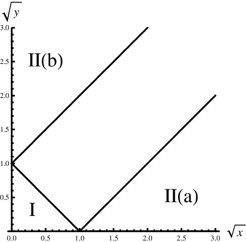
Note that $\kappa$ behaves as a $t$-type invariant under the scaling Eq. (39). In terms of these quantities the Euclidean region can be divided into three regions

1. 1.

   Region I, where $\sqrt{x_{1}}+\sqrt{x_{2}}<1$.

2. 2.

   Region II(a), where $-\sqrt{x_{1}}+\sqrt{x_{2}}>1$.

3. 3.

   Region II(b), where $\sqrt{x_{1}}-\sqrt{x_{2}}>1$.

A graphical representation of these three regions in the $(x_{1},x_{2})$ plane can be found in Fig. 1. Note that Region I is symmetric in $x_{1}$ and $x_{2}$, whereas Regions II(a) and II(b) exchange their roles under an exchange of $x_{1}$ and $x_{2}$. It is easy to see that Regions II(a) and II(b) can be furthermore characterized by

1. 1.

   Region II(a): $(-t_{1})<(-t_{2})$.

2. 2.

   Region II(b): $(-t_{1})>(-t_{2}).$

Note that the region where $k_{4}$ is soft, $s_{1},s_{2}\rightarrow 0$, corresponds to $x_{1},x_{2}\rightarrow+\infty$ in the $(x_{1},x_{2})$-plane.

References

• [1] V. Del Duca, C. Duhr, and E. W. N. Glover, The five-gluon amplitude in the high-energy limit, [0905.0100].
• [2] C. Anastasiou, Z. Bern, L. J. Dixon, and D. A. Kosower, Planar amplitudes in maximally supersymmetric Yang-Mills theory, Phys. Rev. Lett. 91 (2003) 251602, [hep-th/0309040].
• [3] G. P. Korchemsky and A. V. Radyushkin, Renormalization of the Wilson Loops Beyond the Leading Order, Nucl. Phys. B283 (1987) 342–364.
• [4] N. Beisert, B. Eden, and M. Staudacher, Transcendentality and crossing, J. Stat. Mech. 0701 (2007) P021, [hep-th/0610251].
• [5] L. Magnea and G. Sterman, Analytic continuation of the Sudakov form-factor in QCD, Phys. Rev. D42 (1990) 4222–4227.
• [6] G. Sterman and M. E. Tejeda-Yeomans, Multi-loop amplitudes and resummation, Phys. Lett. B552 (2003) 48–56, [hep-ph/0210130].
• [7] Z. Bern, L. J. Dixon, and V. A. Smirnov, Iteration of planar amplitudes in maximally supersymmetric Yang-Mills theory at three loops and beyond, Phys. Rev. D72 (2005) 085001, [hep-th/0505205].
• [8] Z. Bern, M. Czakon, D. A. Kosower, R. Roiban, and V. A. Smirnov, Two-loop iteration of five-point N = 4 super-Yang-Mills amplitudes, Phys. Rev. Lett. 97 (2006) 181601, [hep-th/0604074].
• [9] F. Cachazo, Sharpening The Leading Singularity, [0803.1988].
• [10] L. F. Alday and J. Maldacena, Comments on gluon scattering amplitudes via AdS/CFT, JHEP 11 (2007) 068, [0710.1060].
• [11] Z. Bern et al., The Two-Loop Six-Gluon MHV Amplitude in Maximally Supersymmetric Yang-Mills Theory, Phys. Rev. D78 (2008) 045007, [0803.1465].
• [12] F. Cachazo, M. Spradlin, and A. Volovich, Leading Singularities of the Two-Loop Six-Particle MHV Amplitude, [0805.4832].
• [13] L. F. Alday and J. M. Maldacena, Gluon scattering amplitudes at strong coupling, JHEP 06 (2007) 064, [0705.0303].
• [14] J. M. Drummond, G. P. Korchemsky, and E. Sokatchev, Conformal properties of four-gluon planar amplitudes and Wilson loops, Nucl. Phys. B795 (2008) 385–408, [0707.0243].
• [15] A. Brandhuber, P. Heslop, and G. Travaglini, MHV Amplitudes in N=4 Super Yang-Mills and Wilson Loops, Nucl. Phys. B794 (2008) 231–243, [0707.1153].
• [16] J. M. Drummond, J. Henn, G. P. Korchemsky, and E. Sokatchev, On planar gluon amplitudes/Wilson loops duality, Nucl. Phys. B795 (2008) 52–68, [0709.2368].
• [17] J. M. Drummond, J. Henn, G. P. Korchemsky, and E. Sokatchev, Conformal Ward identities for Wilson loops and a test of the duality with gluon amplitudes, [0712.1223].
• [18] J. M. Drummond, J. Henn, G. P. Korchemsky, and E. Sokatchev, The hexagon Wilson loop and the BDS ansatz for the six- gluon amplitude, [0712.4138].
• [19] J. M. Drummond, J. Henn, G. P. Korchemsky, and E. Sokatchev, Hexagon Wilson loop = six-gluon MHV amplitude, [0803.1466].
• [20] C. Anastasiou et al., Two-Loop Polygon Wilson Loops in N=4 SYM, [0902.2245].
• [21] Z. Bern, L. J. Dixon, D. C. Dunbar, and D. A. Kosower, One loop n point gauge theory amplitudes, unitarity and collinear limits, Nucl. Phys. B425 (1994) 217–260, [hep-ph/9403226].
• [22] Z. Bern, L. J. Dixon, D. C. Dunbar, and D. A. Kosower, One-loop self-dual and N = 4 superYang-Mills, Phys. Lett. B394 (1997) 105–115, [hep-th/9611127].
• [23] I. G. Halliday and R. M. Ricotta, Negative Dimensional Integrals. 1. Feynman Graphs, Phys. Lett. B193 (1987) 241.
• [24] R. M. Ricotta, Negative Dimensions in Quantum Field Theory, in J.J. Giambiagi Festschrift (H. Falomir, ed.), p. 350, 1990. IFT/P-33/89-SAO PAULO.
• [25] H. Exton, Multiple Hypergeometric Functions and Applications. Ellis Horwood, 1976.
• [26] A. P. Prudnikov, Y. A. Brychkov, and O. Marichev, Integrals and Series. Gordan and Breach, 1990.
• [27] A. Erdélyi, Higher Transcendental Functions, vol. 1 and 2. McGraw-Hill, 1954.
• [28] U. Aglietti, V. Del Duca, C. Duhr, G. Somogyi, and Z. Trocsanyi, Analytic integration of real-virtual counterterms in NNLO jet cross sections I, JHEP 09 (2008) 107, [0807.0514].
• [29] Appell, P. and Kampé de Fériet, J., Fonctions Hypergéométriques et Hypersphériques, Polynômes d’Hermite. Gauthiers-Villars, 1926.
• [30] N. N. Bogoliubov and D. V. Shirkov, Quantum Fields. Benjamin Cummings Pub. Co., 1982.
• [31] C. Itzykson and J. B. Zuber, Quantum Field Theory. McGraw-Hill, 1980.
• [32] V. A. Smirnov, Evaluating Feynman Integrals. Springer Tracts Mod. Phys. 211, 2004.
• [33] V. A. Smirnov, Feynman Integral Calculus. Springer, 2006.
• [34] S. Moch and P. Uwer, XSummer: Transcendental functions and symbolic summation in Form, Comput. Phys. Commun. 174 (2006) 759–770, [math-ph/0508008].
• [35] J. A. M. Vermaseren, Harmonic sums, Mellin transforms and integrals, Int. J. Mod. Phys. A14 (1999) 2037–2076, [hep-ph/9806280].
• [36] S. Moch, P. Uwer, and S. Weinzierl, Nested sums, expansion of transcendental functions and multi-scale multi-loop integrals, J. Math. Phys. 43 (2002) 3363–3386, [hep-ph/0110083].
• [37] Z. Bern, M. Czakon, L. J. Dixon, D. A. Kosower, and V. A. Smirnov, The Four-Loop Planar Amplitude and Cusp Anomalous Dimension in Maximally Supersymmetric Yang-Mills Theory, Phys. Rev. D75 (2007) 085010, [hep-th/0610248].
• [38] V. Del Duca, C. Duhr, and E. W. N. Glover, Iterated amplitudes in the high-energy limit, JHEP 12 (2008) 097, [0809.1822].
• [39] T. Gehrmann and E. Remiddi, Numerical evaluation of harmonic polylogarithms, Comput. Phys. Commun. 141 (2001) 296–312, [hep-ph/0107173].