Multiple-Bases Belief-Propagation Decoding
of High-Density Cyclic Codes Thanks: Parts of the results were presented at the IEEE International Symposium on Information Theory (ISIT), Nice, France, 2007. The work was supported in part by the NSF grant CCF 0644427 awarded to Olgica Milenkovic.

Classical algebraic codes of short block length have large minimum distance and efficient soft-decision decoding algorithms [1, 2, 3]. Consequently, these codes represent a good choice for low-delay applications where high transmission reliability is required. Algebraic codes are also frequently used as components of product codes and parts of concatenated coding schemes. In modern storage and communication systems, low-density parity-check (LDPC) codes are most often used as the inner coding scheme. For this reason it is desirable to implement a soft-input soft-output decoder for algebraic codes as a belief-propagation (BP) algorithm. This is a reasonable choice as the decoder can handle both types of codes. Since algebraic block codes have dense parity-check matrices with a large number of short cycles [4, 5], BP decoders offer poor error-correcting performance for such codes.

The use of redundant parity-check matrices for iterative decoding schemes when signaling over the binary erasure channel (BEC) has been excessively studied. Several authors proposed using a high number of redundant checks [6, 7, 8, 9] to improve the decoding performance. This type of decoding has also drawn the attention of researchers who studied this concept in the context of the AWGN channel. Other authors proposed adaptive BP algorithms [10, 11], which iteratively optimize the matrix representation during the decoding process. Such schemes have large implementation complexity due to the required matrix reduction after each iteration. The random redundant decoding (RRD) [4] algorithm does not require this type of processing and obtains very promising results. This is accomplished by serially altering the applied matrix representation within the decoding process. Another closely related approach was described in [12], where a simple simulation-based study using randomly chosen parity-check matrices of the $[24,12,8]$ extended Golay code was performed. This approach offers poor performance when compared both to the performance of the RRD algorithm and the algorithms described in this work.

The approach followed in this paper draws upon the prior work of the authors on BEC decoding [13] and introduces a novel decoding method that operates in parallel and iterative fashion on a collection of parity-check matrices. Using this set of decoder representations, the algorithm performs joint output processing in order to estimate the transmitted codeword. This output processing can occur at various stages of decoding and it may have various degrees of complexity. We distinguish between techniques where the BP algorithms run separately and compare them to schemes where the decoders are allowed to exchange information. In the latter case, we investigate processing of the form of metric and complexity selection, averaging of probabilities [14], information combining [15], as well as certain reliability-based schemes.

As the different representations of the parity-check matrix form bases of the dual code, we refer to the proposed approaches as Multiple-Bases Belief-Propagation (MBBP) decoding. For the purpose of MBBP decoding, one needs to identify classes of parity-check matrices that jointly offer good decoding performance. In order to accomplish this task, we propose using parity-check matrix design techniques originally developed for the BEC but subsequently used for signaling over the AWGN channel. This approach leads to good performance results, as observed both by the authors and other researchers [16]. Moreover, this method relies on the fact that the performance of a parity-check matrix for the BEC is completely characterized by combinatorial entities termed stopping sets [17]; and, that pseudocodewords for linear programming decoders of several classes of channels represent stopping sets for any channel in the Tanner graph [18, 19]. Although we focus our attention on parity-check matrix construction techniques for cyclic codes, the described concepts can be generalized for other classes of codes as well.

The main differences between the existing RRD algorithm and the proposed MBBP scheme are that RRD operates in a serial fashion in terms of periodically permuting the received word, while MBBP works in a parallel manner. Further, the RRD algorithm uses message scaling processing between iterations that tends to increase the overall complexity of the scheme. Contrary, the MBBP algorithm deploys the standard update rules defined by message passing decoding within its parallel cores. Finally, the RRD algorithm uses a greedy search over the Tanner graphs to find a representation which offers good performance as well as random shuffling techniques of the variable nodes. The MBBP algorithm relies on specially designed parity-check matrix families for a given code.

The paper is organized as follows. Section 2 introduces relevant definitions and terminology, while Section 3 contains a description of the bases selection process. Section 4 presents a set of different variations of MBBP decoding algorithms. Simulation results are presented in Section 5.

We start by introducing the terminology related to stopping sets and the BEC. We also provide the terminology needed for describing the MBBP decoding approach.

When transmitting over the BEC, stopping sets completely determine the failure modes of iterative decoders. For completeness we define these sets below [17].

Clearly, a codeword is a stopping set and consequently the size of the smallest stopping set of any given parity-check matrix cannot exceed $d$.

In order to compare different parity-check matrix representations with respect to their decoding performance, we restrict our attention to a simple evaluation criteria: the number of stopping sets of size less than or equal to $\sigma$, for some predefined value $1\leq\sigma\leq d$. Given a parity-check matrix $\textstyle H$, the number of its stopping sets of size $\sigma$ will henceforth be denoted by $\left|{\mathcal{S}}_{\sigma}\left({\mathchoice{\mbox{\boldmath$\displaystyle H$}}{\mbox{\boldmath$\textstyle H$}}{\mbox{\boldmath$\scriptstyle H$}}{\mbox{\boldmath$\scriptscriptstyle H$}}}\right)\right|$. Although stopping sets are known to completely characterize the performance of iterative decoders only for the BEC, they also represent a partial performance indicator for transmission over the AWGN channel. This is due to the intimate connection between stopping sets and pseudocodewords [18, 20].

As we focus our attention on codes with parity-check matrices of cyclic form, a code category that includes cyclic codes, we also provide the following definitions.

For a code with at least one parity-check matrix of cyclic form, we introduce the notion of a partition of the set of codewords of ${\mathcal{C}}^{\perp}$ and the notion of a cyclic orbit generator (cog).

Throughout the paper we focus our attention on cogs of minimum Hamming weight. Little technical modifications are required in the above definition to encompass parity-check matrices that are of cyclic form when restricted to a proper subset of columns, e.g. extended cyclic codes.

Let ${\mathcal{G}}$ be the set of cyclic orbit generators with Hamming weight equal to the minimum distance of the dual code, $d^{\perp}$. A cyclic orbit generator $\mathrm{cog}\,_{\ell}\in{\mathcal{G}}$, $\ell=1,\dots,\left|{\mathcal{G}}\right|$, is used to construct a parity-check matrix ${\mathchoice{\mbox{\boldmath$\displaystyle H$}}{\mbox{\boldmath$\textstyle H$}}{\mbox{\boldmath$\scriptstyle H$}}{\mbox{\boldmath$\scriptscriptstyle H$}}}_{\ell}$, $\ell=1,\dots,\left|{\mathcal{G}}\right|$, of size $m\times n$, $n-k\leq m\leq n$, such that the row-rank of the matrix is $n-k$¹¹ 1 Here, and throughout the paper, we only consider cogs that generate parity-check matrices with row-rank $n-k$. As a consequence, we use the word bases to describe the underlying matrices, although the considered structures are actually frames. Frames are over-complete systems in which every element of a vector space can be represented in a not necessarily unique manner [21].. This matrix consists of $m$ consecutive right shifts of $\mathrm{cog}\,_{\ell}$. To avoid identical rows in ${\mathchoice{\mbox{\boldmath$\displaystyle H$}}{\mbox{\boldmath$\textstyle H$}}{\mbox{\boldmath$\scriptstyle H$}}{\mbox{\boldmath$\scriptscriptstyle H$}}}_{\ell}$ even if $m=n$ holds, only cogs with a period of $n$, i.e. cogs with a cyclic orbit that consists of $n$ distinct shifts, are considered for the construction process.

Note that a redundant parity-check matrix of cyclic form can have at most $n$ distinct rows²² 2 Cyclic matrices with $m=n$ rows are also referred to as circulant matrices.. The larger the value of $m$, the larger the hardware implementation complexity of the BP decoder. Nevertheless, based on extensive computer simulations, it was observed that for decoding of algebraic codes signaled over the AWGN channel the best decoding performance is achieved for $m=n$. This finding holds for both the bit error rate ($\mathrm{BER}$) and frame error rate ($\mathrm{FER}$). The reason supporting this observation is intuitively clear. Consider a parity-check matrix of cyclic form for which $m=n-k$, as shown in (1) for $m=3,n=7$. Here, the symbol $x$ serves as placeholder for the bits of the generating cog of the matrix.

As can be seen from (1), not all of the seven bits participate in the same number of parity-check equations - the column degrees of the parity-check matrix vary with the column. There exist at least two bits (including the first and last) that participate in only one parity-check, and therefore have very low probability of being correctly decoded. Depending on the particular choice of the cog, the set of symbols at the beginning and at the end of the codeword is strongly restricted with respect to the maximum number of parity-checks it can participate in. This problem can be solved by setting $m=n$: such a row-redundancy allows for achieving equal error protection for all code symbols [22]. Therefore, square parity-check matrices will be used throughout the remainder of this paper.

We conclude this section by introducing the notion of a cog family of a set of parity-check matrices.

Recall that a linear $[n,k,d]$ code ${\mathcal{C}}$ is uniquely defined by a parity-check matrix $\textstyle H$ of rank $n-k$ or a generator matrix $\textstyle G$ of rank $k$. There usually exists a large number of generator and parity-check matrices for the same code. For BP decoding over AWGN channels, one usually seeks a sparse parity-check matrix $\textstyle H$. The performance of the algorithm strongly depends on some additional structural properties of $\textstyle H$, such as the number and weight of pseudocodewords.

Adding redundant rows to parity-check matrices improves the performance of iterative decoding for the BEC, but usually has detrimental effects on BP decoders correcting data signaled over the AWGN channel. This can be attributed to the increase of the number of short cycles and the density of the matrix. But, as was shown by the authors in [23], adding judiciously chosen redundant rows may increase the minimum weight of pseudocodewords (and trapping sets) of the given parity-check matrix.

In order to exploit the benefits offered by redundant parity-check matrices with respect to pseudocodeword performance, while controlling the negative effects on the cycle lengths, the following approach can be used. Rather than decoding a received word in terms of only one parity-check matrix, one can use a collection of parity-check matrices, each with small row-redundancy, in parallel. The results of the decoders operating on different parity-check matrices can then be appropriately combined. This is the main idea behind MBBP decoding, and for this purpose, we propose to develop good heuristic techniques for identifying parity-check matrices which offer both good individual and joint decoding performance.

For cyclic algebraic codes, we proved in a companion paper [13] that parity-check matrices that consist of cyclic shifts of carefully chosen cogs offer excellent stopping set properties [24]. In what follows, we focus on identifying families of cogs that obtain very good decoding performance for the AWGN channel. As already pointed out, the iterative decoding performance of a fixed parity-check matrix used over the AWGN channel is, to a certain extent, strongly correlated with its BEC performance, so that we use the total number of stopping sets of size up to $d$ as our cog family optimization criteria.

Since cogs from the same family define parity-check matrices of cyclic form with identical properties for the BEC and comparable properties for the AWGN channel, it is desirable to identify the family with the best performance and then exclusively use cogs from this family to build matrices for MBBP decoding. Identifying all families along with its members by counting stopping sets in the corresponding matrices is computationally expensive [25]. Also, storing all cogs used for decoding can be prohibitively costly, especially for long codes and MBBP decoders with many bases. In order to avoid these problems, we propose to use a cog mapping technique that relies on the notion of the automorphism group of a code.

It is straightforward to prove that there exists a set of permutations ${\mathcal{P}}$ in the automorphism group of a cyclic code which map one cog into another cog from the same family. Fixing one cog, and then applying a subset of permutations from ${\mathcal{P}}$ to it, represents a convenient way for generating redundant parity-check matrices with identical densities and comparable performance under MBBP decoding.

We provide next a partial characterization of the set $\mathcal{P}$ for cyclic codes. More precisely, we describe how to find a large set of permutations $\mathcal{P}$ for which $\left|{\mathcal{S}}_{\sigma}\left({\mathchoice{\mbox{\boldmath$\displaystyle H$}}{\mbox{\boldmath$\textstyle H$}}{\mbox{\boldmath$\scriptstyle H$}}{\mbox{\boldmath$\scriptscriptstyle H$}}}_{a}\right)\right|=\left|{\mathcal{S}}_{\sigma}\left({\mathchoice{\mbox{\boldmath$\displaystyle H$}}{\mbox{\boldmath$\textstyle H$}}{\mbox{\boldmath$\scriptstyle H$}}{\mbox{\boldmath$\scriptscriptstyle H$}}}_{b}\right)\right|$, for $\sigma\leq n$, where the generating cogs of ${\mathchoice{\mbox{\boldmath$\displaystyle H$}}{\mbox{\boldmath$\textstyle H$}}{\mbox{\boldmath$\scriptstyle H$}}{\mbox{\boldmath$\scriptscriptstyle H$}}}_{a}$ and ${\mathchoice{\mbox{\boldmath$\displaystyle H$}}{\mbox{\boldmath$\textstyle H$}}{\mbox{\boldmath$\scriptstyle H$}}{\mbox{\boldmath$\scriptscriptstyle H$}}}_{b}$ satisfy $\mathrm{cog}\,_{b}=\kappa(\mathrm{cog}\,_{a})$, and where $\kappa(\cdot)\in{\mathcal{P}}$. Here, $\kappa(\mathrm{cog}\,_{a})$ is used to denote the action of the permutation $\kappa$ on the vector $\mathrm{cog}\,_{a}$. Note that the same framework can be used when only stopping sets up to a size smaller than or equal to $d$ are considered.

It is well known that the automorphism group of a cyclic code contains two classes of permutations [26]:

• $P_{1}$:

  The class of cyclic permutations $\alpha^{0},\alpha^{1},\ldots,\alpha^{n-1}$, where

  	$\displaystyle\alpha:i$	$\displaystyle\to$	$\displaystyle(i+1)\,\,\mathrm{mod}\,n,\;i=0,\ldots,n-1,$
  	$\displaystyle\alpha({\mathchoice{\mbox{\boldmath$\displaystyle c$}}{\mbox{\boldmath$\textstyle c$}}{\mbox{\boldmath$\scriptstyle c$}}{\mbox{\boldmath$\scriptscriptstyle c$}}})$	$\displaystyle=$	$\displaystyle(c_{n-1},c_{0},c_{1},\ldots,c_{n-2}).$

• $P_{2}$:

  The class of permutations $\beta^{0},\beta^{1},\ldots,\beta^{h-1}$, where

  	$\displaystyle\beta:i$	$\displaystyle\to$	$\displaystyle(2\cdot i)\,\,\mathrm{mod}\,n,\;i=0,\ldots,n-1,$		(2)
  	$\displaystyle\beta({\mathchoice{\mbox{\boldmath$\displaystyle c$}}{\mbox{\boldmath$\textstyle c$}}{\mbox{\boldmath$\scriptstyle c$}}{\mbox{\boldmath$\scriptscriptstyle c$}}})$	$\displaystyle=$	$\displaystyle(c_{0}\,c_{(n+1)/2}\,c_{1}\,\ldots c_{(n-1)/2}),$

  and where $h$ denotes the cardinality of the cyclotomic coset of the $n$-th roots of unity that contains one. Above, all subscripts are taken modulo $n$. For extended cyclic codes, the described permutations are only to be applied to the cyclic part of the codeword.

We find the following definition useful for our subsequent derivations.

The following straightforward results provide a partial characterization of the set of permutations $\mathcal{P}$ of cyclic codes. All proofs rely on the fact that $\alpha^{j}\,\theta=\theta\,\alpha^{j^{\prime}}$, for any integer $j$ and some integer $j^{\prime}$, and for $\theta\in\mathcal{A}(n)$, the affine group of order $n$.

The lemma asserts that cyclic permutations commute (up to a cyclic shift) with all affine permutations in a symmetric group.

We conclude that $\mathcal{A}(n)\cap{\mathrm{Aut}}(\mathcal{C})\subseteq\mathcal{P}$: in other words, applying affine transforms from the automorphism group of the code to one chosen cog in the family produces cogs that generate parity-check matrices with identical stopping set distributions. Therefore, the MBBP decoder does not have to store all redundant bases, but rather a set of permutations, along with a low number of cog vectors that are known to have good stopping set properties. Note that this is a desirable property for practical applications: in order to generate a set of matrices with almost identical and good decoding performance, one only needs to determine the stopping set properties of the cog families rather than that of all individual cogs.

Let $\hat{f}$ denote the index of the optimal or near-optimal family. One vector $\mathrm{cog}\,_{\hat{l}}$, $\hat{l}\in{\mathcal{F}}_{\hat{f}}$, and a subset of permutations in ${\mathrm{Aut}}({\mathcal{C}})$ suffice to generate a set of cogs from ${\mathcal{F}}_{\hat{f}}$. Depending on the set of available permutations, multiple cogs may be required to generate all cogs from the family ${\mathcal{F}}_{\hat{f}}$. With all these cogs at hand, one can construct the matrices ${\mathchoice{\mbox{\boldmath$\displaystyle H$}}{\mbox{\boldmath$\textstyle H$}}{\mbox{\boldmath$\scriptstyle H$}}{\mbox{\boldmath$\scriptscriptstyle H$}}}_{\ell}$, $\ell\in{\mathcal{F}}_{\hat{f}}$, required for MBBP decoding, by cyclically shifting the corresponding cogs, cf. Section 2.

For some classes of cyclic codes, stronger results are available on the structure of the automorphism group. For example, it is known that the automorphism group of a primitive BCH code contains the affine group - and BCH cog families are invariant under the action of every element of the affine group. On the other hand, the family of binary extended quadratic residue (QR) codes [26] with lengths $p+1$, where $p$ is a prime, is known to have automorphism groups that contain permutations from the projective special linear group $PSL(p)$. For $p=8m\pm 1$, the elements of this group can be written as

A non-affine permutation in this group transforms cogs from one family into cogs that belong to a different family. As a result, the image of the original cog generates a parity-check matrix with different stopping set properties compared to the one generated by the original cog.

We describe next in more detail the operating principles of the MBBP decoders, and modifications thereof - as depicted in Figure 1 and 2, respectively. The basic components of an MBBP decoder are collections of (possibly redundant) parity-check matrices, and logical units that combine and process outputs of BP decoders operating on the matrices of the collection. We distinguish two basic MBBP architectures: one, which allows information exchange between decoders (MBBP-X) and another, where the decoder outputs are obtained without exchange of information (MBBP-NX). The decoders in the former category have the feature that information on the reliability of the received symbols can be exchanged during the process of iterative BP decoding; decoders in the latter class can only combine their results upon termination of their individual decoding processes. Both types of decoders can be implemented by storing a set of parity-check matrices. However, if only matrices based on one family of cogs are used, one needs to store only a low number of cogs, along with a set of permutations from ${\mathcal{P}}$.

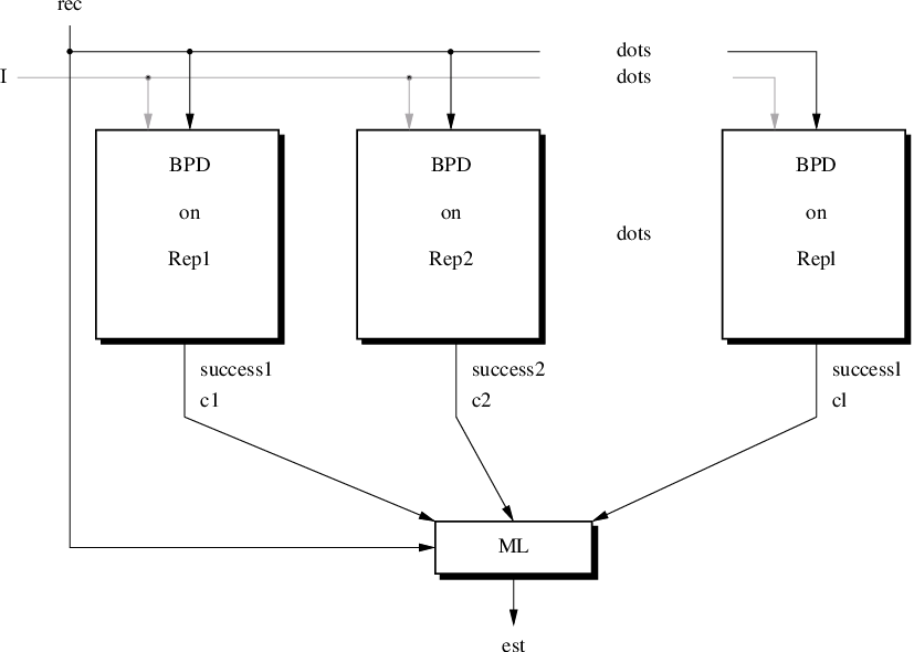
The simplest architecture of an MBBP decoder is depicted in Figure 1, where the outputs of individual decoders are jointly processed only at the end of the decoding cycle. We refer to this technique as standard MBBP decoding (henceforth, MBBP-NX-S decoding).

As already pointed out, parity-check matrices that offer good performance when used for decoding signals transmitted over the BEC may also be good candidates for BP decoding over the AWGN channel [28]. The same characteristic of parity-check matrices was observed through extensive computer simulations for the variants of MBBP decoders, used over the AWGN channel.

In this section, we present performance results for MBBP decoders. Whenever possible, we provide a comparison of the error rates of MBBP decoders with those of a full search algorithm (maximum-likelihood, ML, decoding). If performing full search is computationally infeasible, but results on the weight distribution $\{A_{i}\},i=0,1,\ldots,n$, of the underlying code are available, we plot the union bounds for the $\mathrm{BER}$ and $\mathrm{FER}$ as given by the expressions below:

Here, it is tacitly assumed that the transmitted codeword is the all-zero word, and $A_{i}$ is used to denote the number of codewords of weight $i$ in the given code. Furthermore, we compare our results to the Gallager bound (random coding bound) [29]. This bound considers an ensemble of block codes with length $n$ and rate $R$ and provides a tight upper bound on the average $\mathrm{FER}$, denoted by $\mathrm{E}\{\mathrm{FER}\}$. In this context, the expectation is taken over the ensemble of codes. According to [29], the upper bound reads

where $\rho$, $0\leq\rho\leq 1$, is a design parameter and ${\mathrm{Pr}}({\mathchoice{\mbox{\boldmath$\displaystyle X$}}{\mbox{\boldmath$\textstyle X$}}{\mbox{\boldmath$\scriptstyle X$}}{\mbox{\boldmath$\scriptscriptstyle X$}}})$ denotes the probability vector of the possible channel inputs. Let us specialize this bound for the AWGN channel, which has discrete inputs and an SNR-dependent transition density function $f_{y}(y\mid x_{i})$. Here, $x_{i}$ is chosen from a finite set of cardinality $M_{x}$ and $y$ is a continuous variable, and thus

We illustrate our findings on four short-to-moderate length codes; these codes belong to the class of cyclic and extended cyclic codes, and they include the $[24,12,8]$ extended Golay code, the $[47,24,11]$ quadratic residue (QR) code, the $[31,16,7]$-BCH code, as well as the $[127,64,21]$-BCH code. The maximum number of iterations is set to $N=100$ for all codes and decoding approaches considered. Furthermore, $N_{p}$ is set to $10$ whenever MBBP-X approaches are simulated.

Throughout the remainder of this section, $l$ is used to denote the number of parallel BP decoders in the MBBP architecture. For comparison, simulation results for standard BP decoding are presented as well. Also shown are the performance results of a BP decoder using the union of all parity-check equations in ${\mathchoice{\mbox{\boldmath$\displaystyle H$}}{\mbox{\boldmath$\textstyle H$}}{\mbox{\boldmath$\scriptstyle H$}}{\mbox{\boldmath$\scriptscriptstyle H$}}}_{\ell},\,\ell=1,\dots,l$, simultaneously, for the case of the $[31,16,7]$-BCH code.

We introduced a class of decoding algorithms that operate in parallel on a judiciously chosen family of parity-check matrices. We considered two variants of this class of techniques: one, in which the decoders are not allowed to exchange information during individual runs of the BP algorithm, and another, in which periodic information exchange is allowed. Algorithms in the first class were shown to offer significant performance improvements when compared to the standard BP technique. The approaches in the second class often compare favorably to standard BP, but do not match the performance of algorithms that do not make use of periodic information exchange. Possible reasons for this behavior include the fact that “cycles” are created during the process of information exchange. These cycles “in-between” the graphs of the representations negatively affect the performance of each decoder.

The presented approaches were shown to work for classical high-density codes and are applicable to cyclic and extended cyclic codes. It is possible to generalize the introduced methods to codes like the progressive edge-growth (PEG) [33] family. For this class of codes, significant gains in performance can be obtained [34].

References

- [1] Y. Han, C. Hartmann, and C. Chen, “Efficient maximum-likelihood soft-decision decoding of linear block codes using algorithm A*,” in Proceedings of the IEEE International Symposium on Information Theory (ISIT), (San Antonio, Texas, USA), p. 27, January 1993.
- [2] M. Fossorier and S. Lin, “Soft-decision decoding of linear block codes based on ordered statistics,” IEEE Transactions on Information Theory, vol. 41, pp. 1379–1396, September 1995.
- [3] R. Lucas, M. Bossert, and M. Breitbach, “On iterative soft-decision decoding of linear binary block codes and product codes,” IEEE Journal on Selected Areas in Communications, vol. 16, pp. 276–296, February 1998.
- [4] T. Halford and K. Chugg, “Random redundant soft-in soft-out decoding of linear block codes,” in Proceedings of the IEEE International Symposium on Information Theory (ISIT), (Seattle, Washington, USA), pp. 2230–2234, July 2006.
- [5] T. Halford, A. Grant, and K. Chugg, “Which codes have 4-cycle-free Tanner graphs?,” IEEE Transactions on Information Theory, vol. 52, pp. 4219–4223, September 2006.
- [6] M. Schwartz and A. Vardy, “On the stopping distance and stopping redundancy of codes,” IEEE Transactions on Information Theory, vol. 52, pp. 922–932, March 2006.
- [7] J. Han and P. Siegel, “Improved upper bounds on stopping redundancy,” IEEE Transactions on Information Theory, vol. 53, pp. 90–104, January 2007.
- [8] K. Abdel-Ghaffar and J. Weber, “Complete enumeration of stopping sets of full-rank parity-check matrices of Hamming codes,” IEEE Transactions on Information Theory, vol. 53, pp. 3196–3201, September 2007.
- [9] H. Hollmann and L. Tolhuizen, “On parity-check collections for iterative erasure decoding that correct all correctable erasure patterns of a given size,” IEEE Transactions on Information Theory, vol. 53, pp. 823–828, February 2007.
- [10] A. Kothiyal, O. Y. Takeshita, W. Jin, and M. Fossorier, “Iterative reliability-based decoding of linear block codes with adaptive belief propagation,” IEEE Communications Letters, vol. 9, pp. 1067–1069, December 2005.
- [11] J. Jiang and K. Narayanan, “Iterative soft-input soft-output decoding of Reed-Solomon codes by adapting the parity-check matrix,” IEEE Transactions on Information Theory, vol. 52, pp. 3746–3756, August 2006.
- [12] K. Andrews, S. Dolinar, and F. Pollara, “LDPC decoding using multiple representations,” in Proceedings of the IEEE International Symposium on Information Theory (ISIT), (Lausanne, Switzerland), p. 456, June 2002.
- [13] T. Hehn, O. Milenkovic, S. Laendner, and J. Huber, “Permutation decoding and the stopping redundancy hierarchy of cyclic and extended cyclic codes,” IEEE Transactions on Information Theory, vol. 54, pp. 5308–5331, December 2008.
- [14] S. Laendner and O. Milenkovic, “Algorithmic and combinatorial analysis of trapping sets in structured LDPC codes,” in Proceedings of the International Conference on Wireless Networks, Communications, and Mobile Computing (WirelessComm), (Maui, Hawaii), pp. 630–635, June 2005.
- [15] I. Land and J. Huber, “Information combining,” Foundations and Trends in Communications and Information Theory, vol. 3, pp. 227–330, November 2006.
- [16] L. Zeng, L. Lan, Y. Y. Tai, S. Lin, and K. Abdel-Ghaffar, “Construction of LDPC codes for AWGN and binary erasure channels based on finite fields,” in Proceedings of IEEE Information Theory Workshop (ITW), (Rotorua, New Zealand), pp. 273–276, August 2005.
- [17] C. Di, D. Proietti, I. Telatar, T. Richardson, and R. Urbanke, “Finite-length analysis of low-density parity-check codes on the binary erasure channel,” IEEE Transactions on Information Theory, vol. 48, pp. 1570–1579, June 2002.
- [18] J. Feldman, Decoding Error-Correcting Codes via Linear Programming. PhD thesis, Massachusetts Institute of Technology, Cambridge, MA, USA, 2003.
- [19] C. Kelley and D. Sridhara, “Pseudocodewords of Tanner graphs,” IEEE Transactions on Information Theory, vol. 53, pp. 4013–4038, November 2007.
- [20] R. Koetter and P. Vontobel, “Graph covers and iterative decoding of finite-length codes,” in Proceedings of the 3rd International Symposium on Turbo Codes & Related Topics, (Brest, France), pp. 75–82, September 2003.
- [21] J. Kovacevic and A. Chebira, “Life beyond bases: The advent of frames (Part I),” IEEE Signal Processing Magazine, vol. 24, pp. 86 – 104, July 2007.
- [22] S. Lin and D. Costello, Error Control Coding. Pearson Education, Inc., second ed., 2004.
- [23] S. Laendner, T. Hehn, O. Milenkovic, and J. Huber, “When does one redundant parity-check equation matter?,” in Proceedings of the 49th annual IEEE Global Telecommunications Conference (GlobeCom), (San Francisco, USA), November 2006.
- [24] T. Hehn, S. Laendner, O. Milenkovic, and J. B. Huber, “The stopping redundancy hierarchy of cyclic codes,” in Proceedings of the 44th Annual Allerton Conference on Communication, Control and Computing, (Monticello, USA), pp. 1271–1280, September 2006.
- [25] A. McGregor and O. Milenkovic, “On the hardness of approximating stopping and trapping sets in LDPC codes,” in Proceedings of the IEEE Information Theory Workshop (ITW), (Lake Tahoe, California, USA), pp. 248–253, September 2007.
- [26] F. MacWilliams and N. Sloane, The Theory of Error-Correcting Codes. Amsterdam, The Netherlands: North-Holland Publishing Company, 1977.
- [27] T. Hehn and J. Huber, “LDPC codes and convolutional with equal structural delay: A comparison,” Accepted for publication in IEEE Transactions on Communications, September 2008.
- [28] T. Richardson, M. Shokrollahi, and R. Urbanke, “Design of capacity-approaching irregular low-density parity-check codes,” IEEE Transactions on Information Theory, vol. 47, pp. 619–637, February 2001.
- [29] R. G. Gallager, Information Theory and Reliable Communication. John Wiley and Sons, 1968.
- [30] X.-Y. Hu, M. Fossorier, and E. Eleftheriou, “On the computation of the minimum distance of low-density parity-check codes,” in Proceedings of the IEEE International Conference on Communications (ICC), (Paris, France), pp. 767–771, June 2004.
- [31] T. Hehn, J. Huber, S. Laendner, and O. Milenkovic, “Multiple-bases belief-propagation decoding for short block-codes,” in Proceedings of the IEEE International Symposium on Information Theory (ISIT), (Nice, France), pp. 311–315, June 2007.
- [32] M. Fossorier and S. Lin, “Chase-type and GMD coset decodings,” IEEE Transactions on Communications, vol. 48, pp. 345–350, March 2000.
- [33] X.-Y. Hu, E. Eleftheriou, and D. M. Arnold, “Regular and irregular progressive edge-growth Tanner graphs,” IEEE Transactions on Information Theory, vol. 51, pp. 386–398, January 2005.
- [34] T. Hehn, Optimized Belief-Propagation Decoding for Low-Delay Applications in Digital Communications. PhD thesis, University of Erlangen-Nuremberg, Germany, 2009.