Melting properties of a simple tight-binding
model of transition metals: I. The region of half-filled -band
Abstract
We present calculations of the free energy, and hence the melting properties, of a simple tight-binding model for transition metals in the region of -band filling near the middle of a -series, the parameters of the model being designed to mimic molybdenum. The melting properties are calculated for pressures ranging from ambient to several Mbar. The model is intended to be the simplest possible tight-binding representation of the two basic parts of the energy: first, the pairwise repulsion due to Fermi exclusion; and second, the -band bonding energy described in terms of an electronic density of states that depends on structure. In addition to the number of -electrons, the model contains four parameters, which are adjusted to fit the pressure dependent -band width and the zero-temperature pressure-volume relation of Mo. We show that the resulting model reproduces well the phonon dispersion relations of Mo in the body-centred-cubic structure, as well as the radial distribution function of the high-temperature solid and liquid given by earlier first-principles simulations. Our free-energy calculations start from the free energy of the liquid and solid phases of the purely repulsive pair-potential model, without -band bonding. The free energy of the full tight-binding model is obtained from this by thermodynamic integration. The resulting melting properties of the model are quite close to those given by earlier first-principles work on Mo. An interpretation of these melting properties is provided by showing how they are related to those of the purely repulsive model.
I Introduction
Many years ago, a combination of experiments, first-principles calculations and simple models led to the comprehensive understanding of the low-temperature energetics of transition metals that we have today. [1] Much more recently, advances in experimental and first-principles techniques have started to open the possibility of achieving the same thing for the high-temperature phase diagrams, including melting curves, of transition metals over a wide range of pressures. However, the data obtained so far are fragmentary and sometimes conflicting, [2] and we believe there is now a clear need to develop simple models analogous to those used to interpret low temperature data. These models are needed in order to elucidate the fundamental mechanisms that determine high-temperature phase diagrams, while providing a framework within which to interpret and unify experimental and first-principles data. We describe here how a simple parameterised tight-binding model can be used to calculate the high-temperature free energies of liquid and solid transition metals, and hence their melting properties, and we show how the model can help to interpret the available data. In the present work, we confine ourselves to the case of an approximately half-filled -band, focusing particularly on the interpretation of data for molybdenum.
Shock measurements gave the first experimental information about melting curves at Mbar pressures, and data are available for several transition metals, including Fe, Mo, Ta and W. [3, 4, 5, 6, 7, 8] The thermodynamic states accessible in traditional shock experiments lie on a trajectory called the principal Hugoniot, which provides only a single point on the melting curve. On the other hand, major advances in static compression techniques, based on the diamond anvil cell (DAC), in principle allow entire melting curves and other phase boundaries to be mapped at pressures and temperatures up to GPa and K. Melting data from static techniques have been reported for Fe, Mo, Ta, W, V and Y. [9, 10, 11, 12, 2] There appear to be enormous differences between the melting curves of some transition metals from dynamic and static techniques, with the latter giving much lower melting slopes. The resulting differences of at Mbar pressures can be several thousand K.
Melting curves from first-principles modelling began to appear over 10 years ago, [13, 14] and there are now several well established approaches, including the calculation of solid and liquid free energies, the “reference coexistence” method, and the explicit first-principles simulation of coexisting solid and liquid. [15, 16, 17, 18, 19, 20, 21, 22] For Fe, all three approaches have been used, and the agreement between them is excellent. [23, 24] Since DFT calculations are parameter-free, and reproduce very accurately key quantities such as cold compression curves, phonon frequencies, Hugoniot curves, and the zero-pressure melting temperatures of transition metals, there is every reason to expect that their predictions of melting properties will also be reliable, and there is considerable evidence that this is the case. For transition metals for which static and dynamic measurements disagree seriously, first-principles calculations support the correctness of the dynamic measurements. [25, 30]
Molybdenum is one of the transition metals that have been intensively studied by DFT simulation, and it illustrates the recent controversies. Two independent sets of first-principles calculations [25, 21, 26, 27, 28] agree rather closely with each other and support the high melting curve deduced from shock measurements, this curve rising far more steeply with pressure than the flat melting curve obtained from DAC data. [11] However, the shock measurements [6] also indicate a solid-solid phase boundary, which may be the transition interpreted as melting in the DAC work. [29] A similar conflict between high shock and first-principles melting curves and a low DAC melting curve is also found in Ta, [11, 12, 30] and it has been proposed that the transition seen in DAC may also be a solid-solid transition. We believe that simple models may help to resolve these controversies, by allowing the melting properties of transition metals to be related to the fundamental mechanisms that determine their energetics.
Models for the energetics of transition metals are generally built on the principle that the total energy can be approximated as the sum of the electronic band energy and a repulsive pairwise interaction. The many different models that have been proposed differ mainly in their representation of the band energy. To explain the broad features of transition-metal energetics on a scale of several eV, including the roughly parabolic variations of cohesive energy, lattice parameter and bulk modulus with band filling, it suffices to assume a structureless -band density of states (DOS), whose band width depends only on atomic volume (and chemical element). [31, 1] The simplest total-energy model based on this idea consists of a sum of repulsive pair potentials plus a position-independent bonding term depending on the average atomic volume. We will refer to this as the REP+VOL model. More sophisticated types of total-energy models, including the closely related second-moment, [32] embedded-atom and Finnis-Sinclair models, [33, 34] allow the second moment of the local DOS on each atom to depend on the distances to near neighbours. However, such models do not contain the physics needed to account for the well-known low-temperature structural sequence that occurs through all the transition-metal series, from hexagonal close-packed (hcp), to body-centred cubic (bcc), to hcp, and finally to face-centred cubic (fcc). The energy differences of typically a few tenths of an eV between these structures are clearly essential for any discussion of phase diagrams, but they arise from the structure dependent form of the DOS. There are models that account for this by working with higher moments of the DOS than the second, [1] but a more straightforward approach is to express the total energy function directly in terms of a tight-binding (TB) model. [35, 36] In the present work, we use the simplest possible TB total-energy model, consisting of repulsive pair interactions plus the sum of single-electron energies calculated from a canonical -band TB model, without bands. We refer to this as the REP+TB model. With this simple model, we sacrifice the ability to describe the effect on the DOS of hybridisation, and the pressure dependent transfer of electrons between and bands. We make this sacrifice in order to simplify the analysis.
The principal question addressed in this paper is: What are the main parameters that determine the melting curves and other melting properties of transition metals, and what are the roles of these parameters? As part of this overall question, we would like to know at what level of detail we need to describe the -band bonding. In particular, do we need a detailed description of the structure-dependent electronic DOS in order to understand melting, or is a simpler model, such as REP+VOL, sufficient? In trying to answer these questions, our strategy will be to relate the melting properties of the REP+TB models to those of the pure REP model.
Ultimately, we want to use parameterised tight-binding models to achieve a systematic overall understanding of the melting properties of the entire family of transition metals. However, even the simple models used here require rather extensive calculations to treat melting for a single metal, and for that reason we confine ourselves here to a narrow range of -band filling in the region of half filling. We shall present a simple scheme for fixing the parameters of our model by fitting to zero-temperature first-principles data, and we shall see that, for the case of Mo treated here, we reproduce high-temperature first-principles results reasonably well.
The remainder of the paper is organised as follows. In Section II, we present our REP+TB model for the total energy function, and we describe the scheme we use to fix the model parameters using information from K DFT calculations. In Section III, we present a variety of tests of the model against DFT, both at K and for high-temperature solid and liquid Mo. The procedures used to calculate the free energies of the pure REP and REP+TB systems are described in Section IV, where we also report our results for the melting curves and the volume and entropy of melting. This is followed in Section V by an analysis of the relationships between the melting properties of the REP and REP+TB systems. Discussion and conclusions are in Section VI .
II The tight-binding total-energy model
The total energy of our tight-binding (TB) model for a system of atoms having position is:
| (1) |
where is a repulsive pair potential and . In conventional TB treatments, the energy represents the sum of single-electron energies of occupied states, but here we include the effect of thermal excitation of electrons, so that is actually a free energy, defined as:
| (2) |
where is the Fermi-Dirac occupation number of energy eigenstate at temperature , and is the electronic entropy, given by:
| (3) |
The factors of 2 in Eqns (2) and (3) account for spin. The TB Hamiltonian used to calculate the is described next, and the repulsive pair potential is described after that.
II.1 The canonical -band tight-binding Hamiltonian
Since we include only -electrons in our model, the Hamiltonian matrix elements (, label atoms, , label atomic orbitals) characterize hopping transitions of electrons between the d-orbitals , , , , on each atom. We employ an orthogonal TB model, in which . The dependence of the matrix elements on interatomic distance is taken to be exponential, so that:
| (4) |
The factor depends on the unit vector in the direction from to , and it is well known that it can be expressed in terms of three basic matrix elements dd, dd and dd. Here, we assume the canonical ratios [37] dd : dd : dd = : : . For convenience, and without loss of generality, we assume the diagonal elements to be zero. In order to simplify the numerical simulations, we cut off the matrix elements so that they vanish beyond a distance . The exponential is replaced by a cubic polynomial in the interval , the polynomial coefficients being chosen to ensure continuity of and its first derivative at and . For the Mo model developed here, we chose Å and Å.
The TB density of states (DOS) , defined as:
| (5) |
is normalized so that . Since the trace of is zero, the first moment of the DOS, defined as:
| (6) |
is zero. To fix the values of and , we require that the second moment of the DOS of our model, defined as:
| (7) |
should agree with the volume dependent -band second moment given by DFT.
To apply this procedure to bcc Mo, we performed DFT calculations using the full-potential linearized augmented plane-wave method (FP-LAPW) [38, 39, 40, 41] as implemented in the WIEN2k code. [42] We used the Wu-Cohen [43] form of generalized gradient approximation (GGA), which is known to perform well for transition metals. [44, 45] Local orbitals are added to the standard LAPW basis in order to describe valence and semicore states. The technical parameters in the calculations were set as in Ref. [45] . The total and projected -channel densities of states were obtained by using the modified tetrahedron method of Blöchl et al. [46], and for the projection we used an atomic sphere radius of typically Å. We found that eV and Å give very good agreement with the DFT results for at and GPa (see Table I) and these values are used throughout this work.
The quantity is closely related to the width of the -band , which is the difference between the lowest and highest energy levels, and respectively, in the -band DOS. In DFT calculations, the bottom of the -band can be determined by direct inspection of the DOS, whereas may be difficult to identify because of hybridization of states with different angular momenta (see Fig. 1). Here we identify with an abrupt drop in the projected -DOS at high energies followed by a smooth continuum. For Mo, we find that at equilibrium and are and eV, respectively, while at a pressure of GPa they are and eV (see Fig. 1). As shown in Table I, these values compare well with the tight-binding results obtained with the and values quoted above.
In order to reproduce the energy difference between the Fermi level and bottom of the -band and the form of the -DOS near , we treat the number of electrons as an adjustable parameter. [47] This is important, since many properties of transition metals are understood in terms of the form of the electronic DOS near the Fermi level (e.g. the relative stability of different structures, electronic specific heat, etc). For Mo, we find that , rather than , reproduces quite well the DFT results over a range of pressures (see Fig. 1). We use this value of , unless stated otherwise.
II.2 The repulsive pair potential
The pair potential is also assumed to have an exponential form:
| (8) |
The parameters and are chosen so as to reproduce as closely as possible the measured - curve of bcc Mo at low temperatures. This is essentially the same as fitting to DFT, since with the Wu-Cohen functional the DFT and experimental - curves are almost identical. The values eV and Å give excellent agreement with experimental data of Ref. [6], and DFT calculations (Fig. 2), and we use them throughout this work. The same spatial cut-off distance and smoothing as used for the Hamiltonian matrix elements is applied to the repulsive pair potential.
III Simulation techniques and tests of the model
III.1 Molecular dynamics simulation
All the calculations on our TB model were performed with the OXON code, [48, 49, 50, 51] using diagonalization of the Hamiltonian for each set of ionic positions. In the molecular dynamics (m.d.) simulations, we used the Verlet algorithm to integrate Newton’s equations of motion, with a typical time step of fs. The total force acting on each atom is the exact derivative of the total energy with respect to its atomic position. Our m.d. simulations were performed in the canonical NVT ensemble, using Andersen’s thermostat to avoid errors due to lack of ergodicity. [52] In using this thermostat, the atomic velocities were randomized by drawing them from a Maxwellian distribution every ps. A typical m.d. run consisted of ps for equilibration, followed by ps for the calculation of averages. The m.d. simulations were performed on a supercell containing atoms, and -point sampling was used to integrate over the first Brillouin zone. Pressure was obtained directly in each run using the virial formula.
III.2 Tests of the model
We have performed a series of zero and finite-temperature tests of our model in order to assess its accuracy compared with first-principles results and experimental data. In our first test, we evaluated the relative stability of the different crystal structures at different volumes. To this end, we computed the energy differences of the hcp and fcc structures with respect to the bcc structure at equilibrium ( Å3/atom) and a pressure of GPa ( Å3/atom) . At equilibrium, we found fcc-bcc and hcp-bcc differences of 0.40 and 0.46 eV with DFT, compared with 0.26 and 0.42 with TB. We thus reproduce correctly the relative zero-pressure stability of the different crystal structures, though we predict the fcc phase to be appreciably more stable than hcp. At GPa, we found fcc-bcc and hcp-bcc differences of 0.30 and 0.32 eV with DFT, compared with 0.42 and 0.30 eV with TB. At this pressure, we thus predict that the energy of the hcp phase is lower than that of the fcc phase, but bcc is correctly predicted to be the most stable structure. We note that at both pressures the agreement between the values of obtained with DFT and TB is very good.
We have also computed the phonon frequencies of bcc Mo at the experimental equilibrium volume Å3/atom . [6] Our calculations are based on the small-displacement method, [53, 54] and we have used a supercell containing atoms and -point grid over the first Brillouin zone. In Fig. 3 , we show our results together with experimental data from Ref. [6] and ab initio calculations from Ref. [25] for comparison; the agreement between the TB curves and the others is unexpectedly good, given the simplicity of our model. We note that the experimental phonon anomaly near the H point is not well reproduced by either TB or DFT. [25, 56] We have calculated the phonon frequencies also for the fcc and hcp structures of our TB model. We find that for and there are always imaginary frequencies, so that these structures are unstable, at least at . It worth noting that for slightly larger values the fcc and hcp phases become stable at high pressures; for instance, for fcc becomes stable at GPa.
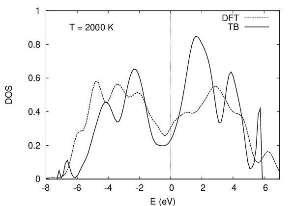
The finite-temperature tests of our model include an analysis of the structure of the solid and liquid at different pressures. In Fig. 4 , we plot the radial distribution function obtained from long (total simulation time ps) DFT and TB m.d. runs. The solid phase is simulated at K and GPa , while the liquid is at K and GPa. (These are states well below and above the melting curve of Mo given by first-principles calculations.) [25, 21] In both phases, the DFT and TB curves agree very well, the main difference being that TB gives interatomic distances slightly smaller than those from DFT simulations.
In Fig. 5 , we show the electronic DOS of solid and liquid Mo obtained at the same thermodynamic conditions as for the radial distribution function. Although the DOS’s obtained with TB and DFT are not identical, the corresponding band-widths and energy differences are very similar, especially for the crystal.
The main conclusion from all these tests is that, in spite of the formal simplicity of our TB model, it reproduces quite reliably many important properties of solid and liquid Mo.
IV Free energy and melting properties of the model
Our overall strategy to obtain the melting properties of our model is based on the calculation of the Helmholtz free energy of the solid and liquid phases. To obtain , we start from the Helmholtz free energy of the purely repulsive system described by the pair potential , and use thermodynamic integration to determine the difference at fixed . This thermodynamic integration is based on the general principle that for total-energy functions and , the difference of the corresponding free energies and at state point is given by
| (9) |
where and denotes the thermal average in the ensemble governed by the total energy function . In practice, we use this type of thermodynamic integration to determine at a set of states, the value of at other states being obtained by integrating the relations and , where and is the total internal energy of the system. The starting point of all the calculations is the free energy of the pure exponential system. Surprisingly, the thermodynamic properties of this system appear not to have been studied before, so we have performed our own calculations of , as described next.
IV.1 Free energy and phase diagram of the pure exponential model
Details of the calculations of the free energy of the pure exponential model will be reported elsewhere, and here we give only a brief summary. Our values of were obtained by thermodynamic integration (Eq. (9)), using as reference system the inverse-6 system interacting with pair potential . We take the Helmholtz free energy of this system from Ref. [57] for the liquid, bcc and fcc phases, and from Ref. [58] for the hcp phase. The thermodynamic integration calculations were performed at a series of points in which the free-energy difference was calculated by averaging over long molecular dynamics runs in which (see Eq. (9)) was varied continuously at a switching rate that guaranteed reversibility (that is, adiabatically). For the solid phase, we considered volumes distributed uniformly over the interval Å3/atom, and the temperature was set to K in all cases. For the liquid phase, points within the same volume range as used for the solid and temperatures taken at intervals of K from initial guessed melting temperatures up to K , were considered. We determined at the other state points by performing thermodynamic integration with respect to pressure and internal energy.
Our calculated values were cross-checked against simulations in which the liquid coexists with the bcc, fcc or hcp solid. These coexistence simulations were performed in the ensemble, and we used the techniques explained in Refs. [25] and [18] . Simulation boxes containing up to atoms were used in the calculations. For each pair of coexisting phases, the pressure dependence of the melting temperature was fitted to the equation
| (10) |
which resembles the so-called Simon equation [59], but is adjusted to ensure that at . Results for the bcc, hcp and fcc melting curves are shown in Fig. 6 . For the bcc melting curve, the values are accurately reproduced with parameters K, GPa and . The volumes and enthalpies per atom of the coexisting solid and liquid were obtained from independent molecular dynamics simulations performed on supercells containing atoms at points on the melting curve. The melting volumes and entropy of fusion for the bcc melting curve are given in Table II. In fact, the melting curves obtained from the coexistence simulations were not perfectly consistent with the Helmholtz free energy results. We have searched carefully for the source of these errors, and we think it is possible that they may come from small imprecisions of the free energies of the inverse-6 system. To correct for these errors, we shifted the free energies of the bcc, hcp and fcc phases with respect to that of the liquid; the corrections depend solely on temperature, and are typically meV/atom. We note that differences between energy shifts of all three crystal structures amount to less than meV/atom, so therefore, total free energy differences between the bcc, fcc, and hcp phases, or equivalently their relative stability, are not affected appreciably by our corrections.
As a further cross-check, we calculated the free energies of the bcc and fcc phases by thermodynamic integration, starting from a different reference system. For this, we took a harmonically vibrating solid, with the harmonic force-constant matrix calculated for a system of particles interacting via the repulsive pure exponential pair potential at volume Å3/atom ( GPa). These calculations are based on the small-displacement method. [53, 54] For both the bcc and the fcc phases, the small discrepancies between the free energies obtained from the inverse-6 and harmonic reference systems are typically meV/atom at temperatures near melting.
IV.2 Free energy and melting properties of the TB model
Our thermodynamic integration calculations to determine the difference were performed by varying adiabatically from to over a time of ps. Simulation boxes containing atoms and -point sampling over the first Brillouin zone were used. The quantity in these calculations (see Eq. (9)) is the TB band free-energy (see Eqs. (2) and (3)). In order to reduce errors due to non-adiabaticity, we perform a complete cycle in which goes from to and back again, and to reduce statistical errors this whole cycle is repeated. The thermodynamic integral is obtained as the average of the values in the four half-cycles. The typical standard deviation of these values is less than meV/atom . An example of the values obtained over a whole run at Å3/atom and temperature K is shown in Fig. 7. We note that varies typically by eV/atom as varies between and .
These thermodynamic integration calculations were performed at ten states in each of the liquid and solid phases. For the solid phase, a temperature of K was chosen for all the volumes; volumes were drawn uniformly from the interval - Å3/atom. For the liquid phase, temperatures of typically K above the melting curve of the repulsive potential were chosen and the same set of volumes as for the solid was used. The value of at the other thermodynamic states was obtained by thermodynamic integration with respect to pressure and internal energy.
In Fig. 8 , we report the melting line of our TB model for -band fillings and , obtained from the Helmholtz free energy calculations described above. We have considered different values in order to assess the effect of this on the melting properties. Since our harmonic calculations showed that only the bcc structure is vibrationally stable, we will report only results for melting from the bcc structure. In practice, once the free energies of the liquid and solid phases are known, we have determined the melting pressure and volumes of the liquid and solid phases at each temperature by the Maxwell double-tangent construction. The Simon formula was then used to fit our results and interpolate at any desired pressure. For , the values of the Simon parameters are K, GPa and . In Table III, we report results for the fractional change of volume and entropy of fusion at points on the melting curves.
In Fig. 8, we also plot the melting curves of the pure exponential system and of Mo obtained from DFT calculations. [25] Although accurate reproduction of real-world data is not the main objective of this work, we note that our model (case ) gives very good agreement with the melting temperatures for Mo of K from experiment [61], and K from DFT simulations. [25] With increasing , significant discrepancies between the TB () and DFT melting curves appear. However, good agreement is partly recovered at high- and high- for .
V Analysis of melting relationships
We pointed out in the Introduction that the gross features of transition metal energetics at K can be understood on the basis of a model in which the structure of the electronic density of states DOS is ignored. This suggests that the simplest possible model for understanding the melting behaviour of transition metals is to add to the free energy of the pure exponential model a bonding term that depends only on volume and does not depend on temperature or on the phase of the system. To test this idea, we have carried out numerical calculations in which we have set equal to the bonding energy contribution to the total energy of the bcc solid at zero temperature (). As expected, varies between and eV/atom over the volume range of interest. The resulting melting curve is shown in Fig. 9 . This very simple model necessarily shifts the melting curve upwards, and our results show that the computed melting temperatures are seriously overestimated, typically by around % . This result shows that there must be a significant dependence of the bonding energy on structure for given volume in the region of the melting curve. To illustrate this, we show in Fig. 10 (Top) the bonding free energy as a function of volume at K for the liquid and bcc solid. Remarkably, the difference between for liquid and solid is rather constant and has a value of eV/atom, being lower in the liquid. This means that the structure dependence of the bonding stabilizes the liquid phase over the solid and therefore lowers the melting curve.
It is interesting to ask whether is significantly influenced by the response of the structure to the presence of the tight-binding energy. To answer this, we show in Fig. 10 (Bottom) the quantity where is the thermal average of evaluated in the ensemble of the potential. The results show that is quite significant in both phases. Moreover, the difference of this quantity for the liquid and solid indicates that the structure of the liquid responds significantly more than the solid to the presence of the TB energy. This effect contributes significantly to the lowering of the melting curve.
VI Discussion and conclusions
The present work is intended as a step towards developing an overall understanding of the phase diagrams of entire transition-metal series over a wide range of pressures and temperatures. At K, generalized phase diagrams (GPD) as a function of pressure and atomic number can be computed by DFT, and we recently reported a phase diagram of this kind for the 4d series. [45] The construction of a complete GPD as a function of , and using DFT is too difficult at present, but we believe that it should be feasible using TB models of the kind described here. With this in mind, it is encouraging that our REP+TB model for Mo, parameterized using only K data, reproduces quite well the melting curve and properties of the high- solid and liquid known from DFT. We have used the same REP+TB model, parameterized using the same scheme, for most of the other 4d metals, and we hope to report - phase diagrams for them in due course. We note that corresponding-states arguments will allow the free energies and melting data for the pure REP model reported here to be used to obtain the free energies of all these transition metals by thermodynamic integration.
Since the properties of Mo over a wide range of and seem to be quite well described by our REP+TB model, it is natural to ask how the melting properties of the model are related to those of the pure REP model, consisting only of exponential repulsion. The melting temperature of REP goes to zero as , so it is clear that the TB energy is crucial in determining the of transition metals at ambient . However, we might expect the repulsion to be increasingly dominant at high . There is an interesting connection here with the melting properties of the Lennard-Jones (LJ) model for rare gases. It was recognised long ago [60] that as , the attractive potential of LJ has diminishing influence on the properties of the coexisting solid and liquid, so that the volume and entropy of fusion tend to those the soft-sphere repulsion model. As we have shown, the melting curves of our REP+TB model for Mo with and do become close to that of pure REP at high . Furthermore, the relative melting volumes of REP+TB for both values decrease steadily with increasing , in a way that is consistent with convergence towards the melting volume of pure REP. However, this convergence is slow, since even at GPa, for REP is 1.1, while for REP+TB it is and 1.5 for and 5.0 respectively. The entropy of fusion is 0.74 for REP over the whole pressure range studied. For , decreases steadily towards this value with increasing , while for it remains a little above this value for all .
In the Introduction, we asked what are the main parameters that determine the melting properties of transition metals. The success of our REP+TB model for Mo suggests that the two parameters and specifying the strength and range of the interatomic repulsion, the strength and range and of the TB matrix elements, and the number of -electrons, may be enough. (Firm conclusions must, of course, await TB calculations on other transition metals.) Our simulations show clearly that a description of the volume-dependent -band width by itself is not enough. The very large d-bonding energy is described by the very simple REP+VOL model, but we have shown that this always raises the melting curve well above that of REP, and gives predictions that agree poorly with the actual melting curves of REP+TB. The melting curves are substantially reduced below those of REP+VOL by the rather small shifts of relative free energies of solid and liquid included in the full REP+TB model. We have seen that a significant contribution to these shifts comes from the response of the system (particularly the liquid) to the presence of the TB energy.
The present work may shed light on recent interpretations of the flat melting curves inferred from DAC measurements. It has been proposed that the directional bonding associated with partially filled -bands may give rise to “preferred local structures” having icosahedral short-range order in the liquid phase. [62, 63] It was suggested that the formation of these local structures lowers the free energy of the liquid, and hence depresses . By contrast with simpler models, such as the embedded-atom model, the TB model we use fully includes directional d-bonding, and our simulated liquid would presumably exhibit the effects of “preferred local structures”, if they were present. The same can be said of the DFT simulations that have been reported on Mo. Nevertheless, both the present TB calculations and the earlier DFT simulations give much steeper melting curves than the DAC measurements, and this indicates that the full inclusion of directional d-bonding does not lead to low melting curves, in contradiction with the suggestions of Refs. [62, 63] .
Our TB model represents only the -band, and ignores the band. This means that, although it mimics the pressure-dependent width of the -band and gives the main features of the DOS, it cannot reproduce the fine details, since it neglects hybridization of d-states with sp-states. It also means that the number of -electrons has to be treated as an adjustable parameter, and we do not include the dependence of this number on pressure or structure. It has been suggested [64] that the dependence of on structure might lead to the very flat melting curves inferred from DAC experiments. However, these ideas are not supported by DFT simulations, which fully include structure-dependent sp-d transfer, but nevertheless give melting curves that rise much more steeply than those from DAC. The fact that the present -band-only TB models give melting curves in reasonable agreement with DFT confirms that sp-d transfer is not expected to give flat melting curves.
A possible resolution of the conflict between shock and first-principles melting curves on one side and DAC melting curves on the other side has emerged recently, at least for some transition metals. [21, 26, 65] DFT simulations of Mo have shown that, although bcc is the most stable structure at low up to over 600 GPa, another structure, perhaps fcc or hcp, is likely to become more stable than bcc at much lower and temperatures well below the melting curve. The suggestion is that the transition interpreted as melting in DAC experiments on Mo may actually be the transition between bcc and this other structure.
Our main conclusions are as follows: A simple tight-binding model, parameterized using data for the volume-dependent -band width and the cold compression curve of Mo reproduces reasonably well the melting curve and the properties of high-/high- solid and liquid Mo known from DFT simulations; the model allows us to analyse the physical mechanisms that determine the melting properties, and to assess suggested explanations for the anomalously low melting curves inferred from static compression experiments. We hope to report soon on TB calculations of melting properties across the whole 4d series.
Acknowledgements.
The work was supported by EPSRC-GB Grant No. EP/C534360, which is 50% funded by DSTL(MOD). The work was conducted as part of a EURYI scheme award to DA as provided by EPSRC-GB (see www.esf.org/euryi).References
- [1] D. Pettifor in Bonding and Structure of Molecules and Solids, Ch. 7 (Clarendon Press, Oxford, 1995).
- [2] D. Errandonea, Physica B 357, 356 (2005).
- [3] C. S. Yoo, N. C. Holmes, M. Ross, D. J. Webb and C. Pike, Phys. Rev. Lett. 70, 3931 (1993).
- [4] J. M. Brown and R. G. McQueen, J. Geophys. Res. 91, 7485 (1986).
- [5] J. H. Nguyen and N. C. Holmes, AIP Shock Compression Condens. Matter 505, 81 (2000).
- [6] R. S. Hixson and J. N. Fritz, J. Appl. Phys. 71, 4 (1992).
- [7] A. C. Mitchell and W. J. Nellis, J. Appl. Phys. 52, 3363 (1981).
- [8] J. H. Nguyen and N. C. Holmes, Nature 427, 339 (2004).
- [9] G. Shen, H. Mao, R. J. Hemley, T. S. Duffy and M. L. Rivers, Geophys. Res. Lett. 25, 373 (1998).
- [10] A. P. Jephcoat and S. P. Besedin, Phil. Trans. R. Soc. A 354, 1333 (1996).
- [11] D. Errandonea, B. Schwager, R. Ditz, C. Gessman, R. Boehler and M. Ross, Phys. Rev. B 63, 132104 (2001).
- [12] D. Errandonea, M. Somayazulu, D. Häusermann and H. K. Mao, J. Phys.: Condens. Matter 15, 7635 (2003).
- [13] G. A. Wijs, G. Kresse and M. J. Gillan, Phys. Rev. B 57, 8223 (1998).
- [14] D. Alfè, M. J. Gillan and G. D. Price, Nature 401, 462 (1999).
- [15] D. Alfè, M. J. Gillan and G. D. Price, Phys. Rev. B 65, 165118 (2002).
- [16] M. J. Gillan, D. Alfè, J. P. Brodholt, L. Vočadlo and G. D. Price, Rep. Prog. Phys. 69, 2365 (2006).
- [17] L. Vočadlo and D. Alfè, Phys. Rev. B 65, 214105 (2002).
- [18] L. Vočadlo, D. Alfè, G. D. Price and M. J. Gillan, J. Chem. Phys. 120, 2872 (2004).
- [19] D. Alfè, M. J. Gillan and G. D. Price, J. Chem. Phys. 116, 6170 (2002).
- [20] D. Alfè, L. Vočadlo, G. D. Price and M. J. Gillan, J. Phys.: Condens. Matter 16, S973 (2004).
- [21] A. B. Belonoshko, L. Burakovsky, S. P. Chen, B. Johansson, A. S. Mikhaylushkin, D. L. Preston, S. I. Simak and D. C. Swift, Phys. Rev. Lett. 100, 135701 (2008).
- [22] D. Alfè, Phys. Rev. B 68, 064423 (2003).
- [23] D. Alfè, G. D. Price and M. J. Gillan, J. Phys. Chem. of Solids 65, 1573 (2004).
- [24] D. Alfè, unpublished.
- [25] C. Cazorla, M. J. Gillan, S. Taioli and D. Alfè, J. Chem. Phys. 126, 194502 (2007).
- [26] C. Cazorla, D. Alfè and M. J. Gillan, Phys. Rev. Lett. 101, 049601 (2008).
- [27] C. Cazorla, M. J. Gillan, S. Taioli and D. Alfè, J. Phys.: Conf. Series 121, 012009 (2008).
- [28] A. B. Belonoshko, S. I. Simak, A. E. Kochetov, B. Johansson, L. Burakovsky and D. L. Preston, Phys. Rev. Lett. 92, 195701 (2004).
- [29] Z. Xiu-Lu, C. Ling-Cang, C. Jun, X. Ji-An and J. Fu-Qian, Chinese Phys. Lett. 25, 2969 (2008).
- [30] S. Taioli, C. Cazorla, M. J. Gillan and D. Alfè, Phys. Rev. B 75, 214103 (2007).
- [31] J. Friedel in The Physics of Metals, ed. J. M. Ziman (London: Cambridge University Press, 1969).
- [32] D. Tomanek, A. Aligia and C. Balseiro, Phys. Rev. B 32, 5051 (1985).
- [33] M. S. Daw and M. I. Baskes, Phys. Rev. B 29, 6443 (1984).
- [34] M. W. Finnis and J. E. Sinclair, Phil. Mag. A 50, 45 (1984).
- [35] C. M. Goringe, D. R. Bowler and E. Hernández, Rep. Prog. Phys. 60, 1447 (1997).
- [36] J. C. Slater and G. F. Koster, Phys. Rev. 94, 1498 (1954).
- [37] O. K. Andersen, Solid State Communications 13, 133 (1973).
- [38] O. K. Andersen, Phys. Rev. B 12, 3060 (1975).
- [39] D. D. Koeling and G. O. Arbman, J. Phys. F 5, 2041 (1975).
- [40] D. D. Koeling and B. N. Harmon, J. Phys. C 10, 3107 (1977).
- [41] D. Singh, in Planewaves, Pseudopotentials and the LAPW method (Kluwer Academic Publishing, Boston 1994).
- [42] P. Blaha, K. Schwarz, G. K. Madsen, D. Kvasnichka and J. Luitz, WIEN2k: An Augmented Plane Wave plus Local Orbital Program for Calculating Crystal Properties, Technical University of Vienna (2001).
- [43] Z. Wu and R. E. Cohen, Phys. Rev. B 73, 235116 (2006).
- [44] F. Tran, R. Laskowski, P. Blaha and K. Schwarz, Phys. Rev. B 75, 115131 (2007).
- [45] C. Cazorla, D. Alfè and M. J. Gillan, Phys. Rev. B 77, 224103 (2008).
- [46] P. Blöchl, O. Jepsen and O. K. Anderson, Phys. Rev. B 49, 16223 (1994).
- [47] A. T. Paxton, J. Phys. D 29, 1689 (1996).
- [48]
OXON : The Oxford Order-N Tight-Binding Package
at
http://www-mml.materials.ox.ac.uk/facilities/oxon.shtml - [49] C. M. Goringe, D. R. Bowler and E. Hernández, Rep. Prog. Phys. 60, 1447 (1997).
- [50] A. P. Horsfield, A. M. Bratkovsky, D. G. Pettifor and M. Aoki, Phys. Rev. B 53, 1656 (1996).
- [51] A. P. Horsfield, A. M. Bratkovsky, M. Fearn, D. G. Pettifor and M. Aoki, Phys. Rev. B 53, 12694 (1996).
- [52] H. C. Andersen, J. Chem. Phys. 72, 2384 (1980).
- [53] G. Kresse and J. Furthmüller, Europhys. Lett. 32, 729 (1995).
- [54] D. Alfè (1998), PHON program available at http://chianti.geol.ucl.ac.uk/dario .
- [55] J. Zarestky, C. Stassis, B. N. Harmon, K. M. Ho and C. L. Fu, Phys. Rev. B 28, 697 (1983).
- [56] P. Souvatzis and O. Eriksson, Phys. Rev. B 77, 024110 (2008).
- [57] B. B. Laird and A. D. J. Haymet, Molec. Phys. 75, 71 (1992).
- [58] S. Prestipino, F. Sija and P. V. Giaquinta, J. of Chem. Phys. 123, 144110 (2005).
- [59] F. E. Simon and G. Glatzel, Z. Anorg. Allgem. Chem. 178, 309 (1929).
- [60] J-P. Hansen, Phys. Rev. A 2, 221 (1970).
- [61] J. W. Shaner, G. R. Gathers and C. Minichino, High Temp. High Press. 9, 331 (1977).
- [62] M. Ross, R. Boehler and D. Errandonea, Phys. Rev. B 76, 184117 (2007).
- [63] M. Ross, D. Errandonea and R. Boehler, Phys. Rev. B 76, 184118 (2007).
- [64] M. Ross, L. H. Yang and R. Boehler, Phys. Rev. B 70, 184112 (2004).
- [65] A. S. Mikhaylushkin, S. I. Simak, L. Burakovsky, S. P. Chen, B. Johansson, D. L. Preston, D. C. Swift and A. B. Belonoshko, Phys. Rev. Lett. 101, 049602 (2008).
| (GPa) | (K) | (Å3) | (Å3) | (%) | |
|---|---|---|---|---|---|
| (GPa) | (K) | (Å3) | (Å3) | (%) | |
|---|---|---|---|---|---|
Figure Caption List
FIG. 1 : -component of the electronic density of states of bcc Mo calculated at K using DFT and TB at pressures of GPa (top panel) and GPa (bottom panel). The Fermi energy is set to zero (vertical lines).
FIG. 2 : Equation of state of bcc Mo obtained from the present TB model (solid line) and DFT (dashed line); experimental data (dots) from Ref. [6] are shown for comparison
FIG. 3 : Phonon dispersion relations of bcc Mo calculated with the present tight-binding model (solid lines) and DFT (dashed lines) at the experimental equilibrium volume Å-3 . Experimental data (dots) from Ref. [55] are shown for comparison.
FIG. 4 : Radial distribution function of solid bcc Mo at K and GPa from long DFT and TB m.d. runs. Bottom: Radial distribution function of liquid Mo at K and GPa obtained from long DFT and TB m.d. runs.
FIG. 5 : -band electronic density of states calculated by DFT and TB m.d. simulation for bcc Mo at GPa, K (top panel) and for liquid Mo at GPa, K (bottom panel).
FIG. 6 Phase diagram of the pure exponential model obtained from coexisting solid and liquid phase ( , , ) simulations. The solid line in the figure corresponds to the bcc-liquid phase boundary while the dashed and dotted lines are the fcc-liquid and hcp-liquid ones, respectively. Dots simbolize points obtained directly from the phase coexistence simulations.
FIG. 7 : Thermal average of the tight-binding energy as function of in an adiabatic thermodynamic-integration calculation of the free energy difference between the REP+TB and REP systems. The plot shows from a simulation in which executes a double cycle , the rate of variation being ps-1.
FIG. 8 : Melting curve of TB model at -band fillings (dashed line) and (dotted line). The melting curve of the pure exponential model and that of Mo from DFT simulations [25] are show for comparison.
FIG. 9 : Melting curve of the repulsive pure exponential potential (solid line), pure exponential potential plus a bonding energy term depending just on volume (short-dashed line), and full tight-binding model at (long-dashed line) and (dotted line) .
FIG. 10 : Top: Free energy difference of the total tight-binding model and repulsive pure exponential potential in the liquid and solid phases at temperature K and for . Bottom: Quantity in the liquid and solid phases at temperature K and for .