Stacking Gravitational Wave Signals from Soft Gamma Repeater Bursts
Abstract
Soft gamma repeaters (SGRs) have unique properties that make them intriguing targets for gravitational wave (GW) searches. They are nearby, their burst emission mechanism may involve neutron star crust fractures and excitation of quasi-normal modes, and they burst repeatedly and sometimes spectacularly. A recent LIGO search for transient GW from these sources placed upper limits on a set of almost 200 individual SGR bursts. These limits were within the theoretically predicted range of some models. We present a new search strategy which builds upon the method used there by “stacking” potential GW signals from multiple SGR bursts. We assume that variation in the time difference between burst electromagnetic emission and burst GW emission is small relative to the GW signal duration, and we time-align GW excess power time-frequency tilings containing individual burst triggers to their corresponding electromagnetic emissions. Using Monte Carlo simulations, we confirm that gains in GW energy sensitivity of are possible, where is the number of stacked SGR bursts. Estimated sensitivities for a mock search for gravitational waves from the 2006 March 29 storm from SGR 1900+14 are also presented, for two GW emission models, “fluence-weighted" and “flat" (unweighted).
pacs
04.80.Nn, 07.05.Kf 95.85.SzI Introduction
Soft gamma repeaters (SGRs) are promising potential sources of gravitational waves (GWs). They sporadically emit brief ( s) intense bursts of soft gamma-rays with peak luminosities commonly up to erg/s. Three of the five known galactic SGRs have produced rare “giant flare” events with initial bright, short ( s) pulses followed by tails lasting minutes, with peak luminosities between and erg/s. According to the “magnetar” model SGRs are neutron stars with extreme magnetic fields G [1]. Bursts may result from the interaction of the star’s magnetic field with its solid crust, leading to crustal deformations and occasional catastrophic cracking [2, 3, 4] with subsequent excitation of nonradial star modes [5, 6, 7] and the emission of GWs [9, 8, 6, 7]. For reviews, see [10, 11].
The LIGO Scientific Collaboration recently completed a search for transient gravitational waves associated with almost 200 individual electromagnetic SGR triggers [12]. That search did not detect GW, but it explicitly targeted neutron star -modes, placed the most stringent upper limits on transient gravitational wave amplitudes at the time it was published, and set isotropic emission energy upper limits that fell within the theoretically predicted range of some SGR models [7].
In this paper we extend that work and describe a new electromagnetically triggered search method for gravitational waves from multiple SGR bursts. Triggered gravitational wave searches assume that gravitational waves associated with an electromagnetic astrophysical event would reach earth at approximately the same time as light from the event. In addition, source sky location is also known.
Knowledge of time and sky position can be a great advantage to gravitational wave searches [13]. It allows us to calculate the detector response functions, allowing us to estimate more relevant upper limits on GW emission using simulated signals from the source. Also, upper limits are typically lower than for untriggered all-sky searches, largely because they are more robust to loud glitches. Finally, searches can target known astrophysical events. If the distance to the source is known, results can be given in terms of isotropic gravitational wave energy emitted from the source instead of strain amplitude at the detector. This ties the search to the astrophysical source instead of the detector on Earth. All of these advantages apply to searches for gravitational waves from SGR bursts.
The new analysis method described here, “Stack-a-flare,” builds upon the analysis pipeline (“Flare pipeline”) used in [12] and described in [14, 15] by attempting to “stack" potential gravitational wave signals from multiple SGR bursts. To stack bursts, we first generate excess power time-frequency tilings. These are 2-dimensional matrices in time and frequency generated from the two detectors’ data streams. Each tiling element gives an excess power estimate in the GW detector data stream in a small period of time and a small range of frequency . The time range of each tiling is chosen to be centered on the time of one of the target EM bursts in the storm. We then align these tilings along the time dimension so that times of the target EM bursts coincide, and perform a weighted addition according to a particular GW emission model.
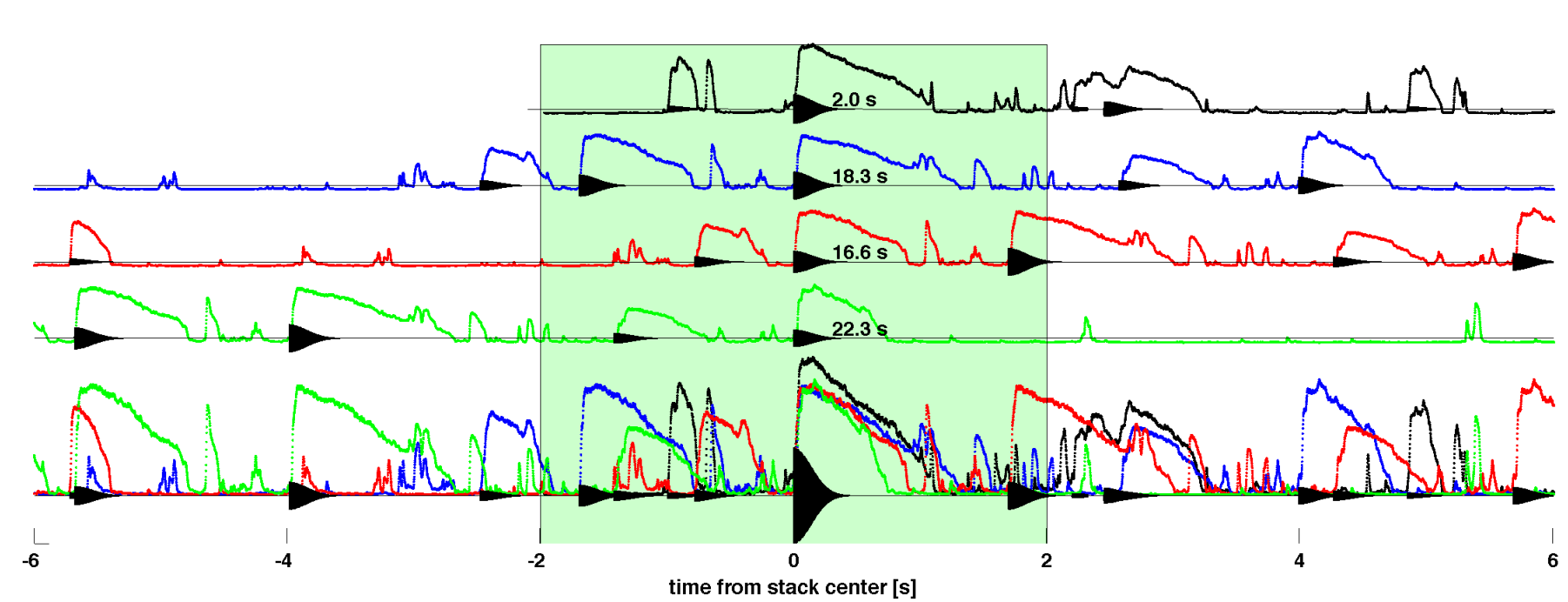
We hope to improve the search sensitivity by combining potential gravitational wave signals from separate bursts in an attempt to increase the signal-to-noise ratio, increasing the probability of detection and placing more stringent constraints on theoretical models via upper limits. We expect that this method would be suitable for performing searches using data from interferometric detectors such as LIGO’s, for gravitational waves associated with SGR storm events such as the 2006 March 29 SGR 1900+14 storm. Figure 1 shows the storm light curve obtained by the BAT detector aboard the Swift satellite [16], and Figure 2 illustrates the stacking procedure with the four most energetic bursts from the storm, showing the main search timescales.
This paper is organized as follows. In Section II we discuss the general strategy of multiple SGR burst searches. In Section III we describe two versions of the analysis method (“Stack-a-flare”), both of which are built upon the Flare pipeline. One version coherently stacks GW time series associated with electromagnetic bursts in the storm, while the other stacks incoherently. We characterize the two versions using simulations in gaussian noise, demonstrating the strengths and weaknesses of each and showing that relatively weak signals which could not be detected in the individual burst search can easily be detected with the new method. Gains in GW energy sensitivity of are feasible with the incoherent version even in the presence of realistic relative timing uncertainties between SGR bursts, where is the number of stacked SGR bursts. Finally, in Section IV we examine the SGR 1900+14 storm light curve of Figure 1 in detail and present estimated search sensitivities for a simulated search for gravitational waves from the storm, for two GW emission models: “fluence-weighted" and “flat" (unweighted).
II Strategy
Before discussing Stack-a-flare method implementation details, in this section we discuss the strategy of a generalized multiple SGR GW search. Due to similarities between the individual burst and multiple burst searches in terms of astrophysics, goals, and implementation, the search choices will be similar to those followed in [12].
II.1 Parameter space of the target GW signals
As in the individual SGR search, multiple SGR searches could target neutron star fundamental mode ringdowns (RDs) predicted in [5, 6, 7, 17] as well as unknown short-duration GW signals. The former are interesting targets because fundamental modes are the modes most efficiently damped by GW emission. The latter are interesting targets because the flare mechanism may involve some other violent motion inside the star, for example matter carried along with magnetic field lines as they rearrange themselves inside the crust. We assume that given a neutron star, -mode frequencies and damping timescales would be similar from event to event, and that unknown signals would at least have similar central frequencies and durations from event to event.
We thus focus on two distinct regions in the target signal time-frequency parameter space. The first region targets (100-400) ms duration signals in the (1–3) kHz band, which includes -mode RD signals predicted in [18] for ten realistic neutron star equations of state. We choose a search band of (1–3) kHz for RD searches, with a 250 ms time window which was found to give optimal search sensitivity [15]. The second region targets (5–200) ms duration signals in the (100–1000) Hz band. The target durations are set by prompt SGR burst timescales (5 ms to 200 ms) and the target frequencies are set by the detector’s sensitive region. We search in two bands: (100–200) Hz (probing the region in which the detectors are most sensitive) and (100–1000) Hz (for full spectral coverage below the RD search band) using a 125 ms time window. In all, we could search in three frequency bands.
We could explore these areas in the parameter space using the same twelve simulated waveform types used for setting upper limits in the individual SGR burst search, described in [12, 15]: linearly and circularly polarized RDs with ms and frequencies in the range 1–3 kHz; and band- and time-limited white noise bursts (WNBs) with durations of 11 ms and 100 ms and frequency bands matched to the two low frequency search bands. Polarization angle will be chosen randomly for every compound injection in initial searches.
It seems plausible to assume that, for a given neutron star, -mode frequencies and damping timescales would be similar from event to event. For pure -modes these quantities depend only on the global structure of the star, essentially the mean density [5], and the magnetic corrections depend on integrals of the field over the entire stellar interior (e.g. [19]). However, the major motivation for the low frequency unknown-waveform portion of the parameter space is stochastic gravitational wave emission arising from violent events in the neutron star crust. Therefore, we will not assume similar waveforms from event to event in the unknown-waveform portion, although we will assume similar central frequencies and durations.
II.2 On-source region
In a search, we divide the GW data into an on-source time region, in which GWs associated with a given burst could be expected, and a background time region. On-source and background segments are analyzed identically resulting in lists of analysis events.
For the individual SGR search, trigger timing precision on the order of a second was handled with 4 s on-source regions. For a multiple SGR search, significantly higher precision in relative trigger times between burst events in the stack will be required. However, a common bias in trigger times shared by all bursts in the stacking set (absolute timing) can be handled with an adequately large (e.g. 4 s) on-source region.
In general, imprecision in trigger times comes principally from two sources: satellite to geocenter light crossing delay and arbitrariness of the satellite trigger point in the light curve. It is possible to decrease both uncertainties through careful analysis of satellite data. If necessary, light crossing times at satellites can be propagated to the geocenter (and subsequently to any given interferometer) using the appropriate ephemeris. If satellite data is public, light curve analysis can yield a specific timing point, for example the start of the steep burst rise. Increased absolute timing precision could allow us to use smaller on-source regions with durations set by theoretical predictions of time delay between electromagnetic and gravitational wave emission from SGR bursts. However, this could exclude astrophysical models with larger timing delays, for instance if the initial excitation transfers energy to the -mode through some slow and inefficient mode-mode coupling due to selection rules. And it turns out there is little benefit to be gained: We have performed Monte Carlo simulations comparing s and s on-source regions. Reducing the on-source region from 4 s to 2 s resulted in only a 2% reduction in amplitude upper limits, on average over 24 trials with various waveform types.
We make one new assumption about the nature of individual bursts of gravitational waves from SGRs: that the time delay between each gamma-ray burst and the associated GW burst does not vary by more than about 100 ms, less than duration of the shortest coherently modeled signal and comparable to the star’s Alfvén crossing time. A variation this large would severely degrade detection efficiency in the case of 11 ms duration WNBs, but as we shall see in Section III.6, detection of neutron star RDs (with s) remains robust.
II.3 Background region
As with the individual burst search, the background region serves three purposes [14, 15]:
- 1.
it is used to estimate statistics of the power tiling as a function of frequency for use in the Flare pipeline;
- 2.
it provides false alarm rate (FAR) estimates from which the significance of the loudest on-source analysis event can be determined;
- 3.
it is representative noise into which simulated waveforms can be injected for estimating upper limits.
In the course of validating the individual SGR search we showed that 1000 s of data on either side of an on-source region produce sufficient estimates of the power tiling statistics [15]. This requirement and the estimation procedure are unchanged in the multiple SGR search, so s of data will again suffice for this purpose. The background region required for injecting simulations to estimate upper limits may depend on the system being modeled and the desired statistical precision; for the mock SGR 1900+14 storm search we describe below, s of background is sufficient. The background region required for FAR estimates depends on the desired precision of FAR estimates. Estimating the FAR of a very large on-source analysis event requires a larger background than estimating the FAR of a small on-source analysis event, for a given level of precision.
II.4 GW emission models
In a multiple burst search we must choose which bursts to include in the set and how to weight them. Since GW energy is unknown we are left to attempt to choose weightings via other observables which we hope will correlate to it. As with the individual burst search, we assume that the SGR burst sample is comprised of bursts occurring within some specified time range defined by the observatory’s science run schedule, and not necessarily from the same SGR source. We will refer to a set of SGR bursts to be included in the multiple burst search, along with a weighting strategy, as a GW emission model.
We could use Occam’s razor to select GW emission models such as the following:
- s1.
flat model — use every detected and confirmed burst from a given SGR source within the time range, with equal weighting. In practice we need to choose a cutoff on which bursts to include;
- s2.
inclusive model — use every detected and confirmed burst within the time range, from any SGR source, with equal weighting;
- s3.
fluence-weighted model — use every detected and confirmed burst from a given SGR source within the time range, weighted proportional to fluence;
- s4.
use a subset of component bursts from a multi-episodic burst event such as the SGR 1900+14 storm, with some weighting scheme.
We note that the inclusive model s2 could benefit from a search method that was insensitive to variations between SGR sources. For example, we would expect two different sources to have -modes at different frequencies, which may not brighten corresponding pixels in a time-frequency tiling. We do not attempt to solve this problem here.
We can also imagine stacking GW emission models based on specific theoretical models. A theory may predict that there is no correlation between and . Such a prediction corresponds to the flat model and is tested below. Or a theory may predict that there is one emission mechanism with a constant mechanical efficiency, and thus is always proportional to . This is treated in the fluence-weighted model and tested below. A theory may predict that is some more complicated function of , the simplest example being a step function—for instance, a theory that small flares originate from magnetic reconnections far out in the magnetosphere and only large flares from reconnections in or near the star itself [21]. However the Swift/BAT spectra of the SGR 1900+14 storm indicate that the neutron star surface participates in all flares [22], and therefore we do not address such a model below (although it might be interesting at a later date). A theory may also predict that the time delay between electromagnetic and gravitational emission varies from burst to burst. Some variation, up to the target signal durations of tens or hundreds of milliseconds, is accounted for in the searches described below. Larger variations could potentially be treated by sweeping over some range of time delays for each burst, a more complicated search which we do not yet address.
We will neglect for the time being complicating factors such as: multiple injections of energy into a single burst, with possible correlation in gravitational wave emission energy; qualitatively different gravitational wave emission in the case of intermediate flares and common bursts; and beaming issues. We also neglect other possibilities such as correlating with flare peak luminosities or rise times.
III Analysis method
Both versions of the Stack-a-flare pipeline, “T-Stack” and “P-Stack,” consist of an extension to the Flare pipeline [15, 14], a simple but effective search pipeline based on the excess power detection statistic of [23].
III.1 Flare pipeline
The Flare pipeline can process streams of data from either one or two GW detectors. First data is conditioned, then excess power tilings are created, and finally analysis events are constructed via clustering elements in the tilings.
Data conditioning consists of zero-phase digital filtering in the time domain [24], first with a bandpass filter and then with a composite notch filter. The raw calibrated LIGO power spectrum is colored, and is characterized by a sensitive region between 60 Hz to 2 kHz which includes a forest of narrow lines, with increasingly loud noise on either side of the sensitive band. Search sensitivity is increased by removing these insensitive regions from the data, which would otherwise dominate weak signals and destroy bandwidth after transformation to frequency domain. We remove narrow lines associated with the power line harmonics at multiples of 60 Hz, the violin modes of the mirror suspension wires, calibration lines, and persistent narrow band noise sources of unknown origin.
Time-frequency spectrograms are then created from conditioned data for individual detectors from a series of Blackman-windowed discrete Fourier transforms, of time length set by the target signal duration. A tile is an estimate of the short-time Fourier transform of the data at a specific time and frequency. Each column in the tiling corresponds to a time bin of width and each row corresponds to a frequency bin of width , both linearly spaced, with . Adjacent time bins overlap by to guard against mismatch between prospective signals and tiling time bins. Larger overlaps require more computation and do not noticeably improve sensitivity [15].
In a one-detector search, we then have a complex-valued time-frequency tiling from which we calculate the real-valued one-sided PSD for every time bin. To do this we multiply each tile value by its complex conjugate and normalize the result to account for sampling frequency and windowing function. We discard frequency bins outside of the chosen search band.
In a two-detector search, we have two complex time-frequency tilings (one for each detector) from which we calculate
| (1) |
where represents a tiling matrix and and are time and frequency bin indices, and and denote the detector. Here is the gravitational wave crossing time difference between detectors; this term takes care of applying the appropriate time difference between detector data streams in the Fourier space, with the advantage of permitting sub-sample time delays, which significantly increases the sensitivity at higher frequencies. The real part is kept, and normalization is applied as in the one-detector case. To obtain a positive-definite statistic we take the absolute value of each tile; this allows sensitivity to both strongly correlated and strongly anti-correlated signals in the two (potentially misaligned) detectors.
Next, we use off-source data to remove the background noise power from each element of the PSD time-frequency tiling. The elements are fit to a gamma distribution [15], and outliers above a threshold (typically four standard deviations) are discarded. The resulting estimate on the mean is subtracted from each element of the corresponding frequency bin in the PSD matrix, giving a matrix of excess power (or “cross excess power” in the two-detector case).
To create analysis events we use a simple 2-dimensional clustering algorithm, allowing retention of signal energy which might otherwise be fragmented in the case of extended signals in the time-frequency plane. Analysis events correspond to discrete clusters found by the algorithm, and include information on cluster central frequency, central time, bandwidth, duration, and so forth. The detection statistic (event loudness) is the sum over the cluster of tile significance.
III.2 T-Stack-a-flare pipeline
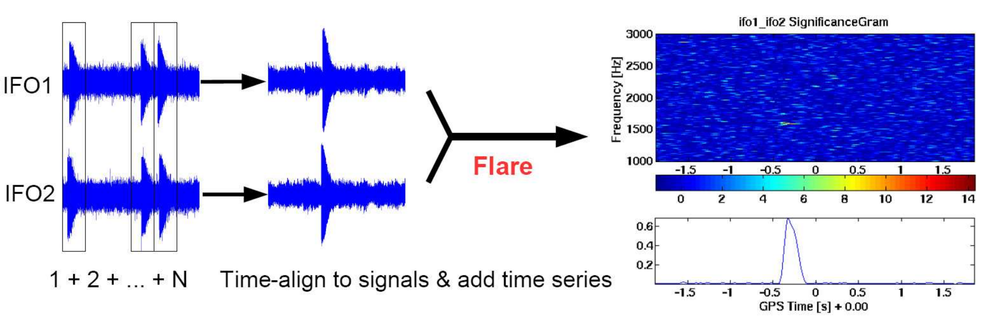
The T-Stack pipeline combines burst events in the time domain.
For each of burst events a trigger time is determined. For a given GW detector, time series segments containing those trigger times are then aligned to the trigger times, weighted according to antenna factor, and added together. The resulting summed time series (either one or two, depending on how many detectors are included in the search) are then fed to the Flare pipeline.
As will be described below, the T-Stack pipeline has the advantage of achieving higher sensitivity in gaussian noise, but the disadvantage of being extremely sensitive to timing inaccuracies and variations in GW signal waveform from burst to burst.
This makes it a potentially viable choice for analyzing multi-episodic events — in which a single contiguous 100 s-binned light curve might provide adequate timing precision — but a poor choice for analyzing isolated burst events or incoherent signals such as band-limited WNBs.
III.3 P-Stack-a-flare pipeline
The P-Stack pipeline combines burst events in the frequency domain.
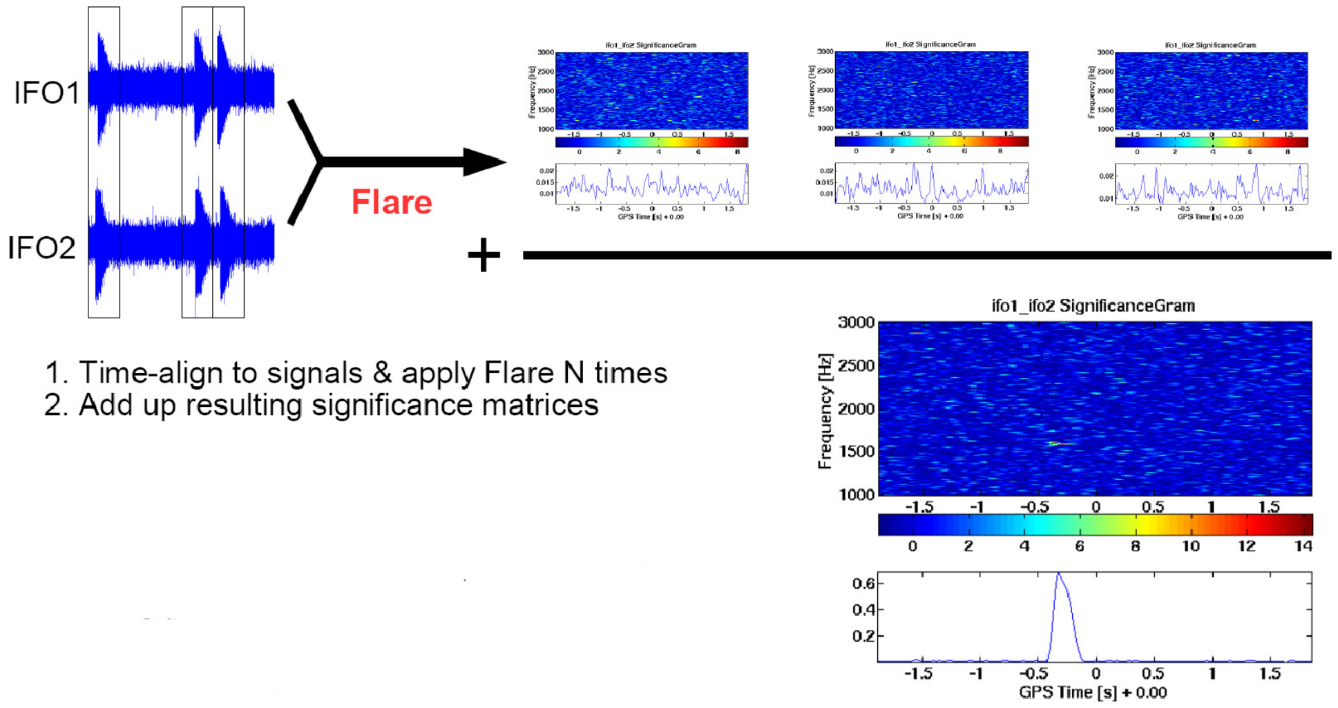
We determine a trigger time for each of burst events based on gamma-ray data. Each of time series containing those triggers is processed with the Flare pipeline, up to the clustering algorithm, exactly as in an individual SGR burst search. Antenna factors are applied at this time. The result is time-frequency significance tilings, with different noise but hopefully with similar or identical signals. The significance tilings are then aligned to the trigger time and added together. The combined significance tiling is then fed through the Flare pipeline clustering algorithm with a fixed fraction of tiles to include in the clustering (e.g. 0.1%). A fixed fraction of tiles is used instead of a fixed loudness threshold value because the variance of the tile loudness distribution at a given frequency increases with .
As will be described below, the P-Stack pipeline has the advantage of being relatively insensitive to timing inaccuracies or differences in waveform from burst to burst, but it has less sensitivity than the T-Stack pipeline for the (possibly unrealistic) precisely-known timing case, with deterministic waveforms.
III.4 Loudest event upper limits
As in the individual SGR search, in the absence of a detection we can estimate loudest event upper limits [25] on GW root-sum-squared strain incident at the detector, and GW energy emitted isotropically from the source assuming a nominal source distance.
We estimate loudest-event upper limits [25] on GW root-sum-squared strain incident at the detector. We can construct simulations of impinging GW with a given . Following [26]
| (2) |
where e.g.
| (3) |
and are the two GW polarizations. The relationship between the GW polarizations and the detector response to an impinging GW from a polar angle and azimuth and with polarization angle is:
| (4) |
where and are the antenna functions for the source at [27]. At the time of the storm, the polarization-independent RMS antenna response , which indicates the average sensitivity to a given sky location, was 0.39 for LIGO Hanford observatory and 0.46 for the LIGO Livingston observatory.
We can also set upper limits on the emitted isotropic GW emission energy at a source distance associated with and via [28]
| (5) |
The upper limit is computed in a frequentist framework following the commonly used procedure of injecting simulated signals in the background data and recovering them using the search pipeline (see for example [29, 30]).
An analysis event is associated with each injected simulation, and compared to the loudest on-source analysis event. The GW strain or isotropic energy at e.g. 90% detection efficiency is the strain or isotropic energy at which 90% of injected simulations have associated events louder than the loudest on-source event.
“Efficiency curves” are constructed by the Flare pipeline by repeatedly analyzing 4 s background segments, each containing a single simulation created with a range of values, and comparing the loudest simulation analysis event within 100 ms (for RDs) or 50 ms (for WNBs) of the known injection time to the loudest on-source analysis event [15]. An example efficiency curve is shown in Figure 5. The range of values must be chosen so that the smallest value produces simulations that are always lost in the noise, and the largest value produces simulations that are typically detected with large signal-to-noise ratios. The or value at 90% detection efficiency ( or ) occurs where 90% of the loudest simulation analysis events are larger than the loudest on-source event.
For any given on-source region this results in four arrays of numbers, each of which has length equal to the number of injected simulations used to estimate the upper limit. The first contains the values of injected simulations. The second contains the calculated values of injected simulations, or if the distance to the source is not known. The third contains the loudness of the analysis event associated with the injected simulation. The fourth contains boolean values indicating whether the associated analysis event was larger then the loudest on-source analysis event or not.
The and boolean (or the and boolean) arrays can be used to construct the efficiency curve, with the (or ) values on the x-axis. The y-axis indicates the fraction of analysis events associated with an injected simulation of as given by the x-axis which are louder than the loudest on-source event. In the case of simulation values which range over a discrete set of scale factors, the y-axis value is simply this fraction. Binomial error bars may be added to these data points.
However, we are typically interested in the or value, that is the of simulations whose associated analysis event is louder than the loudest on-source analysis event 90% or 50% of the time. Since we don’t know this value ahead of time, it is necessary to interpolate between the values associated with the discrete scale factors; we do this by fitting with a sigmoid function. The Flare efficiency curve fitting routine uses two functions to perform these fits: a four-parameter fit based on the logistics function, and a five-parameter fit based on the complementary error function. The models were chosen on empirical grounds, and details are given in [15].
We can follow the same procedure for the multiple burst search. The only difference is the need to measure the or of a compound injection, instead of a simple (single) injection.
III.5 Sensitivity dependence on
The matched filter amplitude signal-to-noise ratio (SNR) is defined in the frequency domain as [31]
| (6) |
where is the Fourier transform of the signal time series and is the noise power spectral density. Here, the numerator is the square root of the power in the signal. In gaussian noise with zero mean, , a constant. Since the standard deviation of gaussian noise goes as the square root of and the amplitude of identical stacked signals goes as , we expect the SNR of the optimal T-Stack algorithm for the recovery of identical signals from noise to go as .
Whereas the T-Stack pipeline stacks amplitude, the P-Stack pipeline stacks power. The background tiles in the power tiling at each individual frequency bin can be modeled as Gamma-distributed noise [15], for which the variance also goes as , so we expect the power signal-to-noise ratio to increase as . Since the amplitude goes as the square root of the power, we expect the P-Stack amplitude sensitivity to increase as .
We tested these predictions by injecting stacked 1590 Hz 200 ms ringdowns into gaussian noise with . We then constructed efficiency curves determining the injection at 50% and 90% detection efficiency. Each efficiency curve was constructed using 20 amplitude scaling factors and 20 trials at each amplitude. An example efficiency curve is shown in Figure 5. We then fit the 50% and 90% detection efficiency level results as functions of to a two-parameter power law of the form . The results for both the T-Stack and P-Stack pipelines are shown in Figure 6 at 90% detection efficiency. The fit for the T-Stack pipeline gives a sensitivity dependence in amplitude at both detection efficiency levels of nearly ( and for 50% and 90% detection efficiencies respectively), confirming our prediction. This corresponds to an improvement in energy of a factor of . The fit for the P-Stack pipeline gives a sensitivity dependence in amplitude at both detection efficiency levels of nearly ( and for 50% and 90% detection efficiencies respectively), confirming our prediction. This corresponds to an improvement in energy of a factor of .
We repeated the experiment for 100 ms duration 100–1000 Hz band-limited WNBs. In this case, we expected the coherent T-Stack pipeline to underperform the the P-Stack pipeline on these independently-generated stochastic incoherent signals. As expected, we found that the T-Stack pipeline shows no improvement as increases, while the P-Stack pipeline show the same sensitivity dependence seen in the coherent ringdown case ( and for 50% and 90% detection efficiencies respectively) . The results are shown in Figure 7; they illustrate the relative model-independence of the P-Stack pipeline.
III.6 Sensitivity dependence on timing errors
The T-Stack pipeline attains optimal sensitivity gains with increasing because it performs a phase coherent addition of signals. We have shown that the P-Stack pipeline attains its energy sensitivity performance even in the case of stacked signals that are not coherent such as independently-generated white noise bursts. For identical signals such as ringdowns, errors in the relative times between stacked signals cause breakdown of phase coherence.
We performed Monte Carlo simulations using a simulated burst series with equal-amplitude ringdowns, and allowing the timing error to range. We characterized 1090 Hz ms and 2590 Hz ms circularly polarized ringdowns, corresponding to the low and high frequency ranges in the signal parameter space. Timing errors were randomly chosen for each ringdown from a normal distribution with ranging from 10 s to 100 ms, and were applied as a timing shift to the given ringdown. At each timing uncertainty we constructed efficiency curves using 20 amplitude scaling factors and 20 trials at each amplitude.
The results are displayed in Figure 8 (1090 Hz ringdowns) and Figure 9 (2590 Hz ringdowns) at 90% detection efficiency. As expected, the P-Stack method is independent of timing error, up until large timing errors on the order of the signal duration. The T-Stack pipeline, on the other hand, shows a pronounced dependence on timing error, especially in the case of high frequency simulations. Each plot shows data for both T-Stack and P-Stack pipelines, and finds the equal-sensitivity timing error (P-Stack and T-Stack curve intersection point) using polynomial fits.
For the T-Stack pipeline to be effective at 1090 Hz, apparently, timing error must be s at one- sigma. For the T-Stack pipeline to be effective at 2590 Hz, timing error must be s at one-sigma. For the case shown, with no timing error the T-Stack pipeline is about 1.5 times more sensitive than the P-Stack pipeline.


III.7 Implications of the pipeline characterization
We summarize the implications from characterizing the T-Stack and P-Stack pipelines. We envision four possible types of stacked SGR searches:
- 1.
High frequency (1000–3000 Hz) searches for ringdown burst emission, for single SGR storm events (ringdown upper limits);
- 2.
Low frequency (100–1000 Hz) searches for stochastic burst emission, for single SGR storm events (band- and time-limited WNB upper limits);
- 3.
High frequency (1000–3000 Hz) searches for ringdown burst emission, for isolated, time-separated SGR bursts (ringdown upper limits);
- 4.
Low frequency (100–1000 Hz) searches for stochastic burst emission, for isolated, time-separated SGR bursts (band- and time-limited WNB upper limits).
We distinguish storm events from isolated events because it is much easier to get precise relative times for storm events.
We have found that the P-Stack pipeline should be effective in any of these cases, with an energy sensitivity gain over the individual burst search of approximately . The T-Stack pipeline shows an energy sensitivity improvement of approximately , but only if the target signals are coherent, and only if the relative timing between SGR GW burst events can be known to high precision (100 s at 1090 Hz and 50 s at 2590 Hz). As we will see, this timing precision requirement is stringent. In the future we might search for a method of overcoming the T-Stack timing precision limitation, possibly by using additional computational resources to perform time shifts between the time series in the stack.
IV SGR 1900+14 storm mock search
In this section we describe a mock stacking search with the P-Stack pipeline, using simulated LIGO data, for GW associated with the 2006 March 29 SGR 1900+14 storm event. We first describe a procedure for estimating burst start times and fluences from the light curve. We then discuss GW emission models. We finally present sensitivity estimates.
IV.1 Light curve and GW emission models
Data from the BAT detector on the Swift satellite are publicly available. In Figure 1, we show the storm light curve in photon counts in the 15–100 keV band with 1 ms time bins. SGR bursts lasting longer than 500 ms are typically considered “intermediate flares”; the storm contained both intermediate flares and common bursts.
Before choosing GW emission models for stacking, we gathered information from the light curve, most importantly consistent relative burst times. Though the BAT timing resolution is 100 s, additional resolution would not improve our estimates of relative burst times as we shall see. We also measured integrated counts under each burst, a quantity roughly proportional to fluence. These efforts were complicated by overlapping and non-uniform bursts in the noisy light curve. We found that a 30-sample running average of the 1 ms-binned light curve aided aspects of the analysis.
| no. | time | delay | counts | fluence | rise | dur. |
|---|---|---|---|---|---|---|
| [s] | [ms] | [erg cm-2] | [counts/s] | [s] | ||
| 1 | 0.975 0.001 | 17.48 | 1.1e+05 | 5.0e-06 | 1.64e+04 | 0.16 |
| 2 | 1.273 0.002 | 17.46 | 2.9e+04 | 1.4e-06 | 3.30e+04 | 0.06 |
| 3 | 1.973 0.003 | 17.46 | 5.0e+05 | 2.4e-05 | 1.58e+04 | 0.94 |
| 4 | 4.067 0.003 | 17.43 | 2.3e+04 | 1.1e-06 | 1.51e+04 | 0.09 |
| 5 | 4.170 0.006 | 17.43 | 7.9e+04 | 3.7e-06 | 1.08e+04 | 0.15 |
| 6 | 4.423 0.018 | 17.43 | 2.6e+05 | 1.2e-05 | 2.51e+03 | 0.57 |
| 7 | 6.819 0.003 | 17.41 | 9.1e+04 | 4.3e-06 | 1.61e+04 | 0.20 |
| 8 | 7.179 0.001 | 17.40 | 2.4e+04 | 1.1e-06 | 2.10e+04 | 0.08 |
| 9 | 10.883 0.002 | 17.36 | 1.1e+05 | 5.1e-06 | 2.28e+04 | 0.26 |
| 10 | 15.287 0.004 | 17.30 | 2.2e+04 | 1.0e-06 | 9.58e+03 | 0.11 |
| 11 | 15.822 0.003 | 17.30 | 1.8e+05 | 8.4e-06 | 7.45e+03 | 0.47 |
| 12 | 16.603 0.004 | 17.29 | 3.7e+05 | 1.7e-05 | 1.60e+04 | 0.77 |
| 13 | 17.632 0.002 | 17.28 | 3.2e+04 | 1.5e-06 | 2.81e+04 | 0.10 |
| 14 | 18.298 0.009 | 17.27 | 4.7e+05 | 2.2e-05 | 1.08e+04 | 1.22 |
| 15 | 19.718 0.000 | 17.25 | 3.1e+04 | 1.4e-06 | 2.78e+04 | 0.11 |
| 16 | 20.865 0.013 | 17.24 | 1.7e+05 | 8.1e-06 | 3.60e+03 | 0.62 |
| 17 | 22.284 0.011 | 17.22 | 2.9e+05 | 1.4e-05 | 9.43e+03 | 0.57 |
| 18 | 30.335 0.001 | 17.12 | 3.4e+04 | 1.6e-06 | 1.65e+04 | 0.15 |
We chose the point of intersection of the rapid rising edges of each burst with the light curve noise floor as plausible and consistent estimates of the times at which possible progenitor catastrophic neutron star events occurred. So long as GW emission is shifted less than 1.5 s before or after this time, it should be well within the on-source region. We first used a generic peak-finding routine to fit and find approximate peak locations; the smallest peaks were ignored as insignificant given the GW emission stacking models we ultimately chose. Local maxima were found by exploring the neighborhoods around the fitted peaks. Walking left from local maxima, a tuned first derivative threshold was used to determine the top and bottom of each burst’s rising edge. The rising edge between these bounds was then fit with a line. Figure 11 shows the fits on all bursts considered for inclusion in the analysis. We then corrected each burst time for the light travel time to the geocenter using the known SGR 1900+14 sky position and known satellite positions. The light travel delay at the beginning of the light curve is 17.48 ms (arriving at the satellite first) and at the end is 17.12 ms, a change of 0.35 ms over a course of 30.5 s. A histogram of one-sigma uncertainty estimates is shown in Figure 12. These uncertainty estimates were applied individually to respective simulations in the Monte Carlo.
Integrated counts under each burst were also estimated, by walking to the right along the smoothed light curve from peak markers until nearly reaching the noise floor or encountering the beginning of the next burst’s rising edge. The light curve with boundaries used in the integrated counts estimate indicated is shown in Figure 10.
Burst integrated count uncertainties were conservatively though qualitatively estimated to be less than 5%, except for one overlapping burst with a burst rise at about 4.2 s. Uncertainty in the overlapping peak is astrophysical in nature and no larger than 3% of the total storm ßuence. The Konus-Wind team reported a conservative storm total fluence of erg cm-2 in the 20–200 keV range [32]. To convert integrated counts to fluences, we used the most conservative estimate of erg cm-2 and the total integrated counts in the entire storm to obtain fluence per count and thus fluences for each burst in the storm. In doing so we assume bursts exhibit spectral uniformity. We wish to know the absolute fluence in order to set upper limits on . Uncertainty in from integrated counts estimates is negligible compared to the uncertainty from the conversion, and so we simply absorb it there. Burst measurements are given in Table 1.


We chose to explore two GW emission stacking models in this mock search: an flat model which sets GW energy emission constant; and a fluence-weighted model comprised of the 18 brightest bursts in the light curve which sets to be constant. The cutoff in the flat model (making it a step function) is motivated by burst integrated counts (Figure 13). The cutoff in the fluence-weighted model was motivated by Figure 14. Including the most energetic 18 bursts accounts for 95% of the counts in the 42 bursts considered for the analysis. After the 15 most energetic bursts, each additional burst (when ordered by energy) contributes less than 1% to the total. In Monte Carlo simulations we observed only a 3% difference (averaged over amplitude sensitivity estimates set via the 12 injection waveforms) between fluence-weighted models with cutoffs at and .
We chose a fluence-weighted GW emission model to explore the constant- hypothesis. We chose not to pursue GW emission models weighted to e.g. burst peak heights or burst rising edge slopes. The cross-correlation between estimated burst peak counts and burst integrated counts is 0.75 in a normalization where auto-correlations are unity. In the fluence-weighted emission model, assuming that GW emission energy is proportional to fluence we weight compound simulations with the square root of integrated counts, and then normalize so that the weight of the most energetic burst is unity. We weight significance tilings on the other hand according to burst integrated counts before stacking them.

IV.2 Results
In this section we present the results of a mock search with the P-Stack pipeline for GW associated with the 2006 March 29 SGR 1900+14 storm, using simulated data. At the time of the storm, all three LIGO detectors were taking science-quality data. Simulated data modeled on data from the two LIGO 4 km detectors were created from gaussian noise by matching power spectra with the LIGO data in the frequency domain. Therefore, the sensitivity estimates should be similar to upper limit estimates from real data.
In Figure 15 we show example cumulative histograms showing false alarm rates versus analysis event loudness for the background and the stacked on-source region. There are three such plots for each emission model, one per search band. Since the stacked livetime is 4 s here, the loudest on-source event occurs once per 4 s, and is plotted at a y-value of 0.25 Hz. We can estimate the FAR of this loudest on-source analysis from the background.
If only one emission model yields a significant event, or if the case is marginal, we can gain additional information by making a joint statement of probability. We can examine the background probability density function in a 2-dimensional space comprised of duples of loudest events from corresponding background segments analyzed under emission models and , and determine constant probability contours , where is a normalizing constant found with a linear fit of the background scatter plot constrained to pass through the origin. These contours then assign a joint probability to the loudest event duple .
Table 2 shows sensitivity estimates on GW amplitude and GW isotropic emission energy assuming a distance of 10 kpc to SGR 1900+14, at 90% detection efficiency, for the flat model and the fluence- weighted model. Sensitivity estimates from simulated data (in which there could be no GW signal) are produced using the identical procedure for producing upper limit estimates in a real search. Sensitivity estimates with are also shown for the sake of comparison; when the Stack-a-flare pipeline reduces to the individual burst search pipeline (Flare pipeline). Superscripts in Table 2 give a systematic error and uncertainties at 90% confidence. The first and second superscripts account for systematic error and statistical uncertainty in amplitude and phase of the detector calibrations, estimated via Monte Carlo simulations, respectively. The third is a statistical uncertainty arising from using a finite number of injected simulations, estimated with the bootstrap method using 200 ensembles [33]. The systematic error and the quadrature sum of the statistical uncertainties are added to the final sensitivity estimates. Methods used to estimate these uncertainties are further described in [15]. As mentioned in Section IV.1, one-sigma burst timing uncertainties as measured by fits of burst rising edges are built into the Monte Carlo. We present the energy sensitivity estimates graphically in Figure 16.
We also present sensitivity estimates on , a measure of the extent to which an energy upper limit probes the GW emission efficiency. Estimates of , being ratios of energies, do not depend on the distance to SGR 1900+14.
V Discussion and conclusion
We have presented the Stack-a-flare method for searching for GW associated with multiple SGR bursts that extends the individual SGR burst search presented in [12, 15]. We have characterized both the T-Stack and the P-Stack versions of the Stack-a-flare pipeline, demonstrating sensitivity dependence on stacking number and uncertainty in relative timing between bursts. The P-Stack pipeline is robust to timing errors, and we have used it to estimate GW amplitude, isotropic emission energy, and search sensitivities for a mock SGR 1900+14 storm multiple SGR search, using simulated data modeled after LIGO data from the science run which was ongoing at the time of the SGR storm. We considered two GW emission models to inform the stacking: flat with ; and fluence-weighted with .
Two other searches for GWs associated with SGR events, besides [12], have been published previously; neither claimed detection. The AURIGA collaboration searched for GW bursts associated with the SGR 1806 giant flare in the band 850–950 Hz with damping time 100 ms, setting upper limits on the GW energy of erg [34]. The LIGO collaboration also published on the same giant flare, targeting times and frequencies of the quasi-periodic oscillations in the flare’s x-ray tail as well as other frequencies in the detector’s band, and setting upper limits on GW energy as low as erg for quasi-periodic signals lasting tens of seconds [35].
Based on the pipeline characterization, we expect to gain a factor of in energy sensitivity in the flat model over the case. We observe a gain of 3.8 averaged over results obtained with the 12 injection waveforms. Comparing these estimated sensitivities to the individual burst search results for the SGR 1900+14 storm published in [12], which analyzed the entire storm in a single s on-source region, we observe a gain in energy sensitivity of an order of magnitude. The best values of in [12], for the 2004 December SGR 1806–20 giant flare, are in the range – depending on injection waveform. These upper limits are about a factor of lower than the estimated sensitivities presented here. However, the Advanced LIGO detectors promise an improvement in by more than a factor of 10 over S5, corresponding to an improvement in energy sensitivity by more than a factor of 100. A stacking search similar to this mock search in Advanced LIGO data could thus conceivably beat the SGR 1806–20 giant flare upper limits. Furthermore, on 2008 August 22, a new SGR was discovered [36, 37, 38] which may be located at a distance of only 1.5 kpc in the direction of the galactic anti-center [39, 40]. A stacking analysis on bursts from this SGR could therefore gain almost 2 additional orders of magnitude in energy and upper limits.
This method would be suitable for a multiple burst search for GW associated with the SGR 1900+14 storm using real LIGO data. A real search would be similar to the mock search in simulated data presented here, although detector collaborations may choose to explore different or additional stacking emission models. This method would also be suitable for multiple SGR burst searches on isolated bursts spanning months or years. We expect this method to continue to be useful when advanced detectors with greater sensitivity come on line.
Acknowledgements.
LIGO was constructed by the California Institute of Technology and Massachusetts Institute of Technology with funding from the National Science Foundation and operates under cooperative agreements PHY-0107417 and PHY-0757058. The authors are also grateful for the support of the National Science Foundation under grants PHY-0457528/0757982, PHY-0555628, the California Institute of Technology, Columbia University in the City of New York, and the Pennsylvania State University. We are indebted to many of our colleagues for fruitful discussions, in particular Richard O’Shaughnessy for his valuable suggestions. This paper has been assigned LIGO Document Number LIGO-P0900001.References
- [1] R. C. Duncan and C. Thompson, ApJ Lett. 392, L9 (1992).
- [2] C. Thompson and R. C. Duncan, MNRAS 275, 255 (1995).
- [3] S. J. Schwartz et al., ApJ Lett. 627, L129 (2005), eprint astro-ph/0504056.
- [4] C. J. Horowitz and K. Kadau, ArXiv e-prints (2009), eprint 0904.1986.
- [5] N. Andersson and K. D. Kokkotas, MNRAS 299, 1059 (1998), eprint gr-qc/9711088.
- [6] J. A. de Freitas Pacheco, Astronomy and Astrophysics 336, 397 (1998), eprint astro-ph/9805321.
- [7] K. Ioka, MNRAS 327, 639 (2001), eprint astro-ph/0009327.
- [8] J. E. Horvath, Modern Physics Lett. A 20, 2799 (2005).
- [9] B. J. Owen, Phys. Rev. Lett. 95, 211101 (2005), eprint astro-ph/0503399.
- [10] S. Mereghetti, A&A Rev. 15, 225 (2008).
- [11] P. M. Woods and C. Thompson, in Compact Stellar X-Ray Sources, edited by W. G. H. Lewin and M. van der Klis (Cambridge Univ. Press, Cambridge, 2004), eprint astro-ph/0406133.
- [12] B. Abbott et al., Phys. Rev. Lett. 101, 211102 (pages 6) (2008), URL http://link.aps.org/abstract/PRL/v101/e211102.
- [13] B. Abbott et al. (LIGO Scientific), Class. Quant. Grav. 25, 114051 (2008a), eprint 0802.4320.
- [14] P. Kalmus et al., Class. Quant. Grav. 24, S659 (2007), eprint astro-ph/0602402.
- [15] P. Kalmus, PhD thesis, Columbia University (2008), arXiv:0904.4394.
- [16] S. Barthelmy et al., Space Sci. Rev. 120, 143 (2005).
- [17] N. Andersson, Class. Quant. Grav. 20, 105 (2003), eprint astro-ph/0211057.
- [18] O. Benhar, V. Ferrari, and L. Gualtieri, Phys. Rev. D 70, 124015 (2004), eprint astro-ph/0407529.
- [19] K. Glampedakis and N. Andersson, Mon. Not. Roy. Astron. Soc. 377, 630 (2007), eprint astro-ph/0702382.
- [20] http://heasarc.nasa.gov/docs/swift/.
- [21] M. Lyutikov, ApJ Lett. 580, L65 (2002), eprint arXiv:astro-ph/0206439.
- [22] G. L. Israel, P. Romano, V. Mangano, S. Dall’Osso, G. Chincarini, L. Stella, S. Campana, T. Belloni, G. Tagliaferri, A. J. Blustin, et al., ApJ 685, 1114 (2008), eprint 0805.3919.
- [23] W. G. Anderson, P. R. Brady, J. D. Creighton, and É. É. Flanagan, Phys. Rev. D 63, 042003 (2001), eprint gr-qc/0008066.
- [24] R. Hamming, Digital Filters (Dover Publications, New York, 1998).
- [25] P. R. Brady, J. D. E. Creighton, and A. G. Wiseman, Class. Quant. Grav. 21, S1775 (2004), eprint gr-qc/0405044.
- [26] B. Abbott et al. (LIGO Scientific Collaboration), Phys. Rev. D 72, 062001 (2005a).
- [27] K. S. Thorne, in 300 Years of Gravitation, edited by S. W. Hawking and W. Israel (Cambridge University Press, Cambridge, 1987), p. 417.
- [28] S. Shapiro and S. Teukolsky, Black Holes, White Dwarfs, and Neutron Stars (Wiley, New York, 1983).
- [29] B. Abbott et al. (LIGO Scientific Collaboration), Phys. Rev. D 72, 082001 (pages 22) (2005b), URL http://link.aps.org/abstract/PRD/v72/e082001.
- [30] B. Abbott et al. (LIGO Scientific Collaboration), Phys. Rev. D 77, 062004 (pages 22) (2008b), URL http://link.aps.org/abstract/PRD/v77/e062004.
- [31] B. Abbott et al., Phys. Rev. D 69, 122001 (2004).
- [32] S. Golenetskii et al., GRB Coordinates Network 4946 (2006).
- [33] B. Efron, Ann. Statist. 7, 1 (1979).
- [34] L. Baggio, M. Bignotto, M. Bonaldi, M. Cerdonio, L. Conti, M. D. Rosa, P. Falferi, P. Fortini, M. Inguscio, N. Liguori, et al. (AURIGA Collaboration), Phys. Rev. Lett. 95, 139903 (pages 1) (2005), URL http://link.aps.org/abstract/PRL/v95/e139903.
- [35] B. Abbott et al. (LIGO Scientific Collaboration), Phys. Rev. D 76, 062003 (2007), eprint astro-ph/0703419.
- [36] S. T. Holland et al., GRB Coordinates Network 8112 (2008).
- [37] S. Barthelmy et al., GRB Coordinates Network 8113 (2008).
- [38] D. Palmer and S. Barthelmy, GRB Coordinates Network 8115 (2008).
- [39] B. M. Gaensler and S. Chatterjee, GRB Coordinates Network 8149 (2008).
- [40] D. A. Leahy and B. Aschenbach, A&A 293, 853 (1995).
| N=1 | N=11 Flat | Fluence-weighted | |||||||||||||
|---|---|---|---|---|---|---|---|---|---|---|---|---|---|---|---|
| Simulation type | ] | [erg] | ] | [erg] | ] | [erg] | |||||||||
| WNB 11ms 100-200 Hz | 3.9 | 1.4 | 2.3 | ||||||||||||
| WNB 100ms 100-200 Hz | 2.9 | 1.4 | 2.2 | ||||||||||||
| WNB 11ms 100-1000 Hz | 6.6 | 4.0 | 5.8 | ||||||||||||
| WNB 100ms 100-1000 Hz | 6.3 | 4.1 | 6.5 | ||||||||||||
| RDC 200ms 1090 Hz | 9.9 | 4.7 | 6.2 | ||||||||||||
| RDC 200ms 1590 Hz | 13 | 6.2 | 11 | ||||||||||||
| RDC 200ms 2090 Hz | 23 | 9.0 | 16 | ||||||||||||
| RDC 200ms 2590 Hz | 20 | 9.3 | 17 | ||||||||||||
| RDL 200ms 1090 Hz | 16 | 10 | 16 | ||||||||||||
| RDL 200ms 1590 Hz | 32 | 15 | 21 | ||||||||||||
| RDL 200ms 2090 Hz | 35 | 18 | 23 | ||||||||||||
| RDL 200ms 2590 Hz | 51 | 29 | 38 | ||||||||||||