How long can a quantum memory withstand depolarizing noise?
Abstract
We investigate the possibilities and limitations of passive Hamiltonian protection of a quantum memory against depolarizing noise. Without protection, the lifetime of a single qubit is independent of , the number of qubits composing the memory. In the presence of a protecting Hamiltonian, the lifetime increases at most logarithmically with . We construct an explicit time-independent Hamiltonian which saturates this bound, exploiting the noise itself to achieve the protection.
pacs
03.67.Pp,03.67.AcA cornerstone for the majority of applications in quantum information processing is the ability to reliably store quantum information, protecting it from the adversarial effects of the environment. Quantum Error Correcting Codes (QECC) achieve this task by using a redundant encoding and regular measurements which allow for the detection, and subsequent correction, of errors [1, 2, 3, 4]. An alternative approach uses so-called protecting Hamiltonians [5, 6], which permanently act on the quantum memory and immunize it against small perturbations. Its most attractive feature is that, in contrast to QECC, it does not require any active action on the quantum memory, just encoding and decoding operations at the time of storing and retrieving the information. Whereas this approach may tolerate certain types of perturbation [7, 8], it is not clear if it is suitable in the presence of depolarizing noise, something which QECC can deal with.
In this Letter, we give a complete answer to this question. More specifically, we consider the situation where a logical qubit is encoded in a set of qubits and allowed to evolve in the presence of depolarizing noise and a protecting Hamiltonian. The goal is to find the strategy delivering the longest lifetime, , after which we can apply a decoding operation and reliably retrieve the original state of the qubit. By adapting ideas taken from [9], it is established that the lifetime cannot exceed . An analysis of the case in which no protecting Hamiltonian is used presents markedly different behavior depending on whether we intend to store classical or quantum information. Finally, we construct a static protecting Hamiltonian that saturates the upper bound . To this end, we first show how to achieve this bound using a time–dependent Hamiltonian protection which emulates QECC. We then introduce a clock gadget which exploits the noise to measure time–similar to radiocarbon dating–thus allowing us to simulate the previous time dependent protection without explicit reference to time.
We consider a system of qubits, each of which is independently subject to depolarizing noise at a rate . The total state evolves as
| (1) |
Furthermore, we shall allow for an arbitrary encoding of the initial state as well as a final decoding procedure to recover the information.
Protection limitations.—Using purely Hamiltonian protection, a survival time of is the maximum achievable. Intuitively, this is due to the fact that the depolarizing noise adds entropy to the system at a constant rate, while any reversible operation (i.e., Hamiltonian/unitary evolution) will never be able to remove this entropy from the system. Rather, in the best case, it can concentrate all the entropy in a subsystem, keeping the remaining part as clean as possible. This entropic argument was first presented in [9], where the authors investigated the power of reversible computation (both classical and quantum) subject to noise in the absence of fresh ancillas. To this end, they considered the information content of the system, with the number of qubits and . The information content upper bounds the number of classical bits extractable from , and thus ultimately also the number of qubits stored in . While the original statement about the decrease of is for discrete-time evolution, it can be straightforwardly generalized to the continuous time setting of Eq. (1), where it states that
which yields that the information of the system is smaller than after a time .
Having established an upper bound for the scaling of with , let us analyze whether this bound can be reached under different circumstances. We start out with the simplest case where we use no Hamiltonian protection (i.e., ) and show that is independent of ; that is, no quantum memory effect can be achieved. For that, we note that the effect of Eq. (1) on each qubit may be expressed in terms of a depolarizing channel
where . For , where , the resulting channel is entanglement breaking [10]. This remains true if one incorporates encoding and decoding steps. It is simple to prove that for entanglement breaking qubit channels, the average fidelity [11] is upper-bounded by . Thus, the lifetime is smaller than , which is independent of .
The previous argument does not apply to classical information, for which an optimal storage time that is logarithmic in may be achieved. The classical version of Eq. 1, taking , is a system of classical bits subject to bit flipping noise (each bit is flipped at a rate ). In this case, encoding in a repetition code, and decoding via majority voting, yields an asymptotically optimal information survival time . Using optimal estimation [12] and this classical protocol in the encoding phase, the bound may be asymptotically reached for the quantum case.
Time dependent protection.—We will now use the ideas of QECC to build a simple circuit based model that reaches the upper bound on the protection time. This model assumes that unitary operations can be performed instantaneously, which is equivalent to having a time–dependent protecting Hamiltonian with unbounded strength; we will show how to remove both requirements later on. Instead of using a repetition code, we encode the qubit to be protected in an level concatenated QECC [2, 3, 4] (i.e., levels of the QECC nested into each other), which requires qubits, where is the number of qubits used by the code. Each level of the QECC can provide protection for a constant time , and thus, after one layer of decoding needs to be executed. Each decoding consists of a unitary on each -tuple of qubits in the current encoding level; after the decoding, only one of each of the qubits is used further (Fig. 1). The total time that such a concatenated QECC can protect a qubit is given by , as in the classical case.
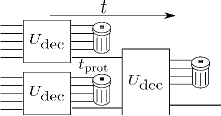
Time-independent protection.—In the following, we show that the same protection time which we can achieve using a time-dependent protection circuit can also be obtained from a time-independent protecting Hamiltonian. The basic idea of our construction is to implement the time-dependent Hamiltonian presented before in a time independent way. To this end, a clock is built which serves as control. The time-independent version performs the decoding gates conditioned on the time estimate provided by the clock. In order to obtain a clock from (1) with a time-independent , we will make use of the noise acting on the system: we add a number, , of “clock qubits” which we initialize to and let the depolarizing noise act on them. The behavior of the clock qubits is thus purely classical; they act as classical bits initialized to which are being flipped at a rate . Thus, the polarization , defined by the number of “” bits minus the number of “” bits has an average expected value of at time . Conversely, this provides the time estimate
| (2) |
Here, is the maximum time for which we expect the estimate to be reliable which depends on and the precision of the estimate, cf. (5) below. Particular realizations of this random process of bit flips can be described by a polarization trajectory . Good trajectories are defined to be those such that
| (3) |
for all . For appropriate parameters and , the following theorem states that almost all trajectories are good and can provide accurate time estimates.
Theorem (Depolarizing clock): For , good trajectories have a probability
| (4) |
Furthermore, for any good trajectory , the time estimate returned by the clock will differ from the real time by at most
| (5) |
(For fixed , this implies that will scale logarithmically with the number of qubits.)
Note that the theorem does not simply state that any time evolution will be outside (3) for an exponentially small amount of time (which is easier to prove), but that there is only an exponentially small number of cases in which (3) is violated at all. Although the former statement would in principle suffice to use the clock in our construction, the stronger version of the theorem makes the application of the clock, and in particular the error analysis, more transparent and will hopefully lead to further applications of the clock gadget.
Proof. To prove the theorem, note that each of the bits undergoes an independent exponential decay, so that the total polarization is the sum of identical independent random variables. We can thus use Hoeffding’s inequality [13] to bound the probability of finding a polarization far from the expected average value ,
| (6) |
This already implies that most of the trajectories violate (3) for no more than an exponentially small amount of time. To see why (6) implies that most trajectories are good trajectories, we bound the average number of times a trajectory leaves the region (3) of good trajectories. Since a non-good trajectory must leave (3) at least once, it is also an upper bound on the probability of non-good trajectories. Hence, it suffices to consider the average rate at which processes leave (3), and integrate over to obtain a bound on the probability of trajectories which are not good.

The rate at which a process leaves the set of good trajectories has two sources, as illustrated in Fig. 2: First, the system can undergo a spin flip, thus leaving the region defined by (3) vertically (rate ), and second, it can leave it horizontally if the time passes the maximum time allowed by (3) for the current value of the polarization (rate ). A vertical leave can occur only if , provided (a spin flip changes by ). Eqn. (6) thus gives an average bound
A horizontal leave can only occur at discrete times extremizing (3),
and the probability of a trajectory fulfilling may again be bounded using (6), such that
The inequality (4) follows immediately by integrating from to .
Assuming that corresponds to a good trajectory, the accuracy of the time estimate (2) may be bounded by applying the mean value theorem to :
Clock dependent Hamiltonian.—Let us now show how the decoding circuit can be implemented using the clock gadget. The circuit under consideration consists of the decoding unitaries (decoding the ’th encoded qubit in level , acting on qubits each); after a time interval (the time one level of the code can protect the qubit sufficiently well), we perform all unitaries at the current level —note that they act on distinct qubits and thus commute. Each of these unitaries can be realized by applying a -qubit Hamiltonian for a time . Thus, we have to switch on all the for , where .
In order to control the Hamiltonian from the noisy clock, we define clock times and , and introduce a time-independent Hamiltonian which turns on the decoding Hamiltonian for level between ,
| (7) |
The left part of the tensor product acts on the code qubits, the right part on the clock (qu)bits, and
where is an -bit string with Hamming weight . The initial state of the system is, as for the circuit construction, the product of the encoded qubit in an -level concatenated code and the maximally polarized state on the clock gadget.
Error analysis.—We now perform the error analysis for the protecting Hamiltonian (7). In order to protect the quantum information, we will require that the error probability per qubit in use is bounded by the same threshold after each decoding step is completed (i.e. at ). We will restrict to the space of good trajectories, since we know from the clock theorem that this accounts for all but an exponentially small fraction, which can be incorporated into the final error probability.
We will choose large enough to ensure that the error in the clock time satisfies . In this way, we ensure that the decoding operations are performed in the right order 11 1 The noisy clock has the potential to run backwards in time within its accuracy. and with sufficient precision. We may thus account for the following error sources between and :
i) Inherited errors from the previous rounds which could not be corrected for. By assumption, these errors are bounded by .
ii) Errors from the depolarizing noise during the free evolution of the system. The system is sure to evolve freely for a time , i.e., the noise per qubit is bounded by .
iii) Errors during the decoding. These errors affect the decoded rather than the encoded system and stem from two sources: On the one hand, the time the Hamiltonian is active has an uncertainty , which gives an error in the implemented unitary of not more than . On the other hand, depolarizing noise can act during the decoding for at most a time . In the worst case, noise on any of the code qubits during decoding will destroy the decoded qubit, giving an error bound . Thus, the error on the decoded qubit is
Since the noise is Markovian (i.e. memoryless), the clock does not correlate its errors in time. In summary, the error after one round of decoding is at most , which we require to be bounded by again. Here, is a property of the code, and returns the error probability of the decoded qubit, given a probability of error on each of the original qubits; for example, for the 5-qubit perfect QECC [14], .
We will now show that it is possible to fulfill the required conditions by appropriately defining the control parameters. First, we choose to have the QECC [14] work well below threshold. We may take and . To minimize imprecision in the implemented unitaries, the decoding Hamiltonians are chosen of minimal possible strength, . Finally we take . Inserting the proposed values in the derived bounds, it is straightforward to show that .
The number of code qubits required is , with . The required logarithmic clock lifetime and the precision are obtained by taking and , by virtue of Eq. (5) of the clock theorem. For any fixed and , this allows a lifetime .
Conclusions.—In this paper, we have considered the ability of a Hamiltonian to protect quantum information from decoherence. While without a Hamiltonian, quantum information is destroyed in constant time, the presence of time-dependent control engenders protection for logarithmic time, which is optimal. As we have shown, the same level of protection can be attained with a time-independent Hamiltonian. The construction introduced a noise-driven clock which allows a time dependent Hamiltonian to be implemented without explicit reference to time.
Since depolarizing noise is a limiting case of local noise models, it is expected that the time-independent Hamiltonian developed here can be tuned to give the same degree of protection against weaker local noise models, although these models may admit superior strategies. For instance, noise of certain forms (such as dephasing) allows for storage of ancillas, potentially yielding a linear survival time by error correcting without decoding. In the case of amplitude damping noise, the noise itself distills ancillas so that the circuit can implement a full fault-tolerant scheme, which gives an exponential survival time, assuming that one can redesign the clock gadget to also benefit from these properties.
Whether the same degree of protection can be obtained from a Hamiltonian which is local on a 2D or 3D lattice geometry remains an open question 22 2 A first step is to incorporate the notion of boundedness. By controlling each decoding unitary in a given round from a different clock (which does not affect the scaling properties), a constant bound to the sum of Hamiltonian terms acting on any given finite subsystem can be shown. . However, intuition suggests this might be impossible; the crucial point in reversibly protecting quantum information from depolarizing noise is to concentrate the entropy in one part of the system. Since the speed of information (and thus entropy) transport is constant due to the Lieb-Robinson bound [15], the rate at which entropy can be removed from a given volume is proportional to its surface area, while the entropy increase goes as the volume. It thus seems impossible to remove the entropy sufficiently quickly, although this argument is not fully rigorous, and the question warrants further investigation.
We acknowledge the DFG for support (projects MAP and FOR635), and the EU (QUEVADIS and SCALA). ASK is also supported by Clare College, Cambridge.
References
- [1] P. Shor, in Foundations of Computer Science, 1996. Proceedings., 37th Annual Symposium on (1996), pp. 56–65.
- [2] D. Aharonov and M. Ben-Or, quant-ph/9611025 (1996).
- [3] D. Gottesman, Phys. Rev. A 57, 127 (1998).
- [4] D. Gottesman, arXiv:0904.2557 (2009).
- [5] A. Y. Kitaev, Annals of Physics 303, 2 (2003).
- [6] D. Bacon, Phys. Rev. A 73, 012340 (2006).
- [7] E. Dennis, A. Kitaev, A. Landahl, and J. Preskill, J. Math. Phys. 43, 4452 (2002).
- [8] R. Alicki, M. Horodecki, P. Horodecki, and R. Horodecki, arXiv:0811.0033 (2008).
- [9] D. Aharonov, M. Ben-Or, R. Impagliazzo, and N. Nisan, quant-ph/9611028 (1996).
- [10] M. Horodecki, P. W. Shor, and M. B. Ruskai, Rev. Math. Phys. 15, 629 (2003).
- [11] M. A. Nielsen, Phys. Lett. A 303, 249 (2002).
- [12] S. Massar and S. Popescu, Phys. Rev. Lett. 74, 1259 (1995).
- [13] W. Hoeffding, J. Amer. Statistical Assoc. 58, 13 (1963).
- [14] R. Laflamme, C. Miquel, J. P. Paz, and W. H. Zurek, Phys. Rev. Lett. 77, 198 (1996).
- [15] E. H. Lieb and D. W. Robinson, Commun. Math. Phys. 28, 251 (1972).