Search for Gravitational Wave Bursts from
Soft Gamma Repeaters
Peter M. Kalmus
Submitted in partial fulfillment of the
requirements for the degree
of Doctor of Philosophy
in the Graduate School of Arts and Sciences
COLUMBIA UNIVERSITY
2008
LIGO-P080079-00-Z
©2008
Peter M. Kalmus
All Rights Reserved
ABSTRACT
Search for Gravitational Wave Bursts from
Soft Gamma Repeaters
Peter M. Kalmus
We present the results of a LIGO search for short-duration gravitational waves associated with soft gamma repeater (SGR) bursts, and a method for calibrating gravitational wave detectors via photon actuators.
Photon calibrators provide an independent calibration of LIGO’s three gravitational wave detectors. Their nominal confidence error bars are currently estimated to be 3%. The photon calibrators have provided a valuable check on the official calibration, uncovering problems that may otherwise have gone unnoticed.
We also present the first gravitational wave search sensitive to neutron star -modes, usually considered the most efficient gravitational wave emitting modes. We find no evidence of gravitational waves associated with any SGR burst in a sample consisting of the 2004 December 27 giant flare from SGR 1806 and 190 lesser events from SGR 1806 and SGR 1900+14 which occurred during the first year of LIGO’s fifth science run. Gravitational wave strain upper limits and model-dependent gravitational wave emission energy upper limits are estimated for individual bursts using a variety of simulated waveforms. The unprecedented sensitivity of the detectors allows us to set the most stringent limits on transient gravitational wave amplitudes published to date. We find upper limit estimates on the model-dependent isotropic gravitational wave emission energies (at a nominal distance of 10 kpc) between and erg depending on waveform type, detector antenna factors and noise characteristics at the time of the burst. These upper limits are within the theoretically predicted range of some SGR models.
Finally, we propose a new method which extends the initial SGR burst search, exploring the possibility that SGR sources emit similarly in gravitational waves from burst to burst by “stacking" potential gravitational wave signals. We show that gains in gravitational wave energy sensitivity of are possible, where is the number of stacked SGR bursts. Estimated sensitivities for a mock search for gravitational waves from the 2006 March 29 storm from SGR 1900+14 are presented for two stacking scenarios: the “fluence-weighted" scenario and the “flat" (unweighted) scenario.
Contents
List of Tables
List of Figures
Acknowledgments
What a privilege it is to do science! I’m grateful to live in a time and a place where I could have this opportunity. Science stands not only on the shoulders of giants, but of all people.
Hundreds of folks in LIGO and at Columbia have helped me fulfill this dream in one way or another. I’m especially grateful to two groups: the people who worked to make the LIGO detectors sensitive enough to allow this work to be interesting; and the Burst Working Group, whose members forced me to defend my ideas and ultimately supported my work. I am also grateful for the support of the United States National Science Foundation under cooperative agreements PHY-04-57528/PHY-07-38147/PHY-07-57982, the LIGO Scientific Collaboration, Columbia University, and the California Institute of Technology.
A handful of individuals have been especially helpful. Foremost among them is my advisor, Szabolcs Márka, who guided me through the perilous phase transitions needed to become a scientist. Szabi rarely lost patience explaining something to me for the time, and provided a foundation on which to do good work. I also owe thanks to Sergey Klimenko at the University of Florida, who was a kind of second advisor. Sergey generously taught me much of what I know about gravitational wave burst analysis. I am grateful to Kipp Cannon and Ben Owen, who formally reviewed the SGR search presented in Chapter 8 on behalf of the LSC, a huge job which they performed efficiently. The work in Chapter 8 relied on S. Barthelmy, N. Gehrels, K. C. Hurley, G. Lichti, S. Mereghetti, D. Palmer, D. Smith, and the Konus-Wind team for electromagnetic SGR burst data. It was a pleasure working with these satellite folks, and I look forward to further collaboration. I thank Yoichi Aso for comments on Chapter 3, and Drew Keppel for comments on Chapter 2. I am grateful to Andy Millis and Amber Miller at Columbia for helping me find my way back to physics. I am also grateful to Lyman Page at Princeton, for showing me that physics is fun, for encouraging me to return to graduate school, and for his benediction as I started this segment of my life: “Do good work.” Finally, and above all, I thank Sharon for putting up with this project as we started our family.
To my parents, who never stop believing in me
And to Sharon, for insight in the dark and celebrating when the light shines down
Chapter 1 The Universe Through New Eyes
We are poised to enter the age of gravitational wave astrophysics. Gravitational waves are perturbations in the spacetime metric propagating at the speed of light, predicted by Einstein in 1914 by his theory of general relativity [1]. In GR, massive objects cause a curvature distortion in four-dimensional spacetime, and gravitational force is our perception of something trying to follow a geodesic in the curved spacetime. When a massive object moves it drags the distortion with it, sending out ripples in spacetime. Due to the weakness of the gravitational force, gravitational waves have not yet been directly detected. An attempt to directly detect gravitational waves, and to extract science from upper limits on gravitational wave emission, is the subject of this work.
We do have indirect evidence for the existence of gravitational waves. In a beautiful observational confirmation of Einstein’s prediction, R. Hulse and J. Taylor measured the time derivative of the orbital period of PSR 1913+16, a pulsar in a binary system with a second neutron star, by observing the Doppler shifting of the pulsar signals due to orbital velocity. They confirmed that the orbital velocity increase due to loss of gravitational potential energy matches what would be expected in general relativity if the system were losing energy due to gravitational wave emission to within experimental precision, better than 0.5% (Figure 1.1) [2, 3, 4, 5, 6]. More recent observations place the agreement to within about 0.2% [7]. These stars will collide and merge in about 300 million years due to losses from gravitational wave emission.

Because of this indirect detection of gravitational waves, and also because of other experimental verifications of general relativity [6], we are confident that gravitational waves do exist. One of the biggest goals in physics today is to directly detect gravitational waves in order to see what the information they carry can teach us about the universe. The science that will come from such a discovery is thrilling to contemplate.
For the first time, the LIGO Scientific Collaboration has gathered more than a year of data with laser interferometric gravitational wave detectors with sensitivities and frequency bands such that a detection might not require an extraordinary event [8]. By 2009 planned upgrades on these detectors are expected to improve amplitude sensitivity by a factor of , and additional upgrades planned to be completed by 2013 will give us advanced detectors about 10 times more sensitive to gravitational wave strain than current detectors, and therefore with about 1000 times the reach in terms of astrophysical volume [9]. Meanwhile, plans for both new and existing detectors in other countries will strengthen the emerging global interferometeric gravitational wave detector network (see Table 1.1). Global networks reduce the false detection rate and improve the source sky localization.
| detector | location | date | arm length [m] |
|---|---|---|---|
| LIGO [10] H1 | Hanford, WA | operational | 4000 |
| L1 | Livingston, LA | operational | 4000 |
| H2 | Hanford, WA | operational | 2000 |
| GEO600 [11] | Hannover, Germany | operational | 600 |
| Virgo [12] | Cascina, Italy | operational | 3000 |
| TAMA300 [13] | Mitaka, Japan | operational | 300 |
| LCGT [14] | Kamioka Mine, Japan | not clear | 3000 |
| LISA [15, 16] | space | 2018 |
Lack of a detection with the network of advanced detectors would be very interesting. The more likely scenario of routine detection may revolutionize astrophysics. Each new portion of the electromagnetic spectrum, when opened to astrophysical observation, has resulted in unimagined discoveries. Observing the universe through gravitational radiation ought to be even more radical than looking with a new color of light. Table 1.2 compares gravitational waves to electromagnetic waves as carriers of astrophysical information.
| characteristic | gravitational wave | electromagnetic waves |
|---|---|---|
| medium | spacetime | space |
| source | coherent quadrupole motions of black holes, stars, galaxies, etc. | incoherent dipole motions of electrons, other charged particles |
| interaction with intervening matter | insignificant; could probe supernova centers, very early universe, etc. | absorbed and scattered by intervening matter; carry information from outer layer of objects only. |
| frequency | Hz | Hz |
| detectors | omnidirectional | unidirectional |
| quantum mechanics | spin 2 graviton | spin 1 photon |
We have contributed to this massive effort in both the hardware and data analysis domains. We have improved the LIGO gravitational wave detectors through advancement of a calibration technique that uses photons to drive the interferometer test masses. In the course of this work we discovered significant discrepancies in measurements of the response function magnitude with the official calibration via coil actuators, which ultimately led to an improved understanding of the detector calibration. We also used the photon calibrators to help uncover a significant error in the official timing calibration.
We have also developed and used novel data analysis techniques to search LIGO data for gravitational wave bursts associated with soft gamma repeaters (SGRs), a bizarre and enigmatic class of astrophysical sources and a promising source for gravitational waves. Soft gamma repeaters sporadically emit short energetic bursts of soft gamma rays. The bursts may be driven by violent interaction between the most intense magnetic fields known in the universe and the solid crust of a neutron star [17, 18]. These catastrophic events could excite the star’s nonradial modes [19, 20, 21] which are damped via gravitational wave emission [22, 23, 20, 21]. We have performed an electromagnetically triggered search for gravitational waves associated with SGR burst events in a sample which includes 214 bursts from the first year of LIGO’s fifth science run (S5y1) and the 2004 December 27 giant flare from SGR 1806–20. This is the first search sensitive to -modes, usually considered the most efficient gravitational wave emitters [19]. The unprecedented sensitivity of the detectors and of our analysis pipeline allows us to set the most stringent limits on transient gravitational wave amplitudes published to date. These upper limits already begin to constrain some SGR models.
There is a possibility that potential gravitational wave emission from SGR bursts is similar from burst to burst. We have also developed a search method which explores this possibility, by attempting to “stack" potential gravitational wave signals from multiple SGR bursts with the aim of digging deeper into the noise and increasing the probability of a detection. This new method extends the individual burst search described in the last paragraph.
This thesis is organized as follows.
In Chapter 2 we give a brief theoretical description of gravitational waves to facilitate understanding of gravitational wave detectors and searches. We also discuss some of the sources of potentially detectable gravitational waves.
In Chapter 3 we briefly describe laser interferometric gravitational wave detectors as implemented by LIGO, the Laser Interferometric Gravitational Observatory. While other types of detectors exist, such as bar[24] and spherical [25] detectors, we believe that interferometric detectors are currently most likely to yield interesting science, and we limit our discussion to them. We focus in particular on the methods used to measure relative length changes in an interferometer that are 1000 times smaller than a proton diameter, the sensitivity required to begin to have some chance of detecting gravitational waves.
In Chapter 4 we describe the LIGO photon calibrator system, and compare photon calibrator measurements to measurements made with the traditional coil calibrators. These measurements revealed a significant discrepancy with the official detector response calibration magnitude. We also describe photon calibrator measurements of the detector timing, which revealed a significant discrepancy with the official timing calibration. We discuss the future utility of photon calibrators in LIGO, suggesting that they could be a candidate for the Advanced LIGO primary calibration system.
In Chapter 5 we describe in detail a simple but powerful general purpose coherent gravitational wave analysis pipeline for externally triggered searches, the Flare pipeline. We present the Flare pipeline as a complete and automated analysis system which, given inputs including data from one or two interferometric gravitational wave detectors and information describing one or more electromagnetic triggers, produces a statement of detection or non-detection and upper limits for a variety of simulation waveform types on gravitational wave strain and isotropic gravitational wave emission energy from the source.
In Chapter 6 we describe careful characterization and validation of the Flare pipeline which was carried out before and during official review by the LIGO Scientific Collaboration (LSC).
In Chapter 7 we describe soft gamma repeaters. Knowledge of SGRs was used in designing a compelling search for gravitational waves associated with their bursts.
In Chapter 8 we describe the search for gravitational waves associated with individual SGR bursts using the Flare pipeline. We describe the sample of SGR triggers and give the results of the search.
In Chapter 9 we describe the search for gravitational waves associated with multiple SGR bursts using the Stack-a-flare pipeline. This is forward-looking work with interesting problems which will benefit from collaboration with the community of SGR theorists. We describe and characterize the pipeline, and we present estimated sensitivities for a mock search for gravitational waves from the 2006 March 29 storm from SGR 1900+14.
Finally, in Chapter 10 we summarize our work, describe potential future extensions, and conclude our thesis.
Chapter 2 Gravitational Waves
In this chapter we give a brief introduction to the theory of gravitational waves. The intention here is to provide a foundation for understanding gravitational wave detectors and data analysis. We then survey interesting potential astrophysical sources of gravitational wave emission.
An introduction to general relativity is given in Schutz [26]; an intermediate treatment is given in Carroll [27]; and a definitive reference is Misner, Thorne and Wheeler [28]. We have followed these texts in our discussion.
2.1 Gravitational waves in general relativity
In general relativity Einstein sought to present a self-consistent theory of gravity in which no frame of reference is favored, based upon the postulates of special relativity: the relativity of velocity and the universality of a finite speed of light. In so doing he revolutionized intuitive conceptions of space and time.
Newton’s theory of gravity predicts instantaneous transmission of information. Einstein’s field equations in general relativity allow wave solutions, with gravity propagating at the speed of light. These gravitational wave solutions are analogous to electromagnetic waves described by Maxwell, and the wave solutions which emerge from the descriptions of gravity and electromagnetism propagate at the same speed.
Though there is a deep connection between the forces, there are major differences on the surface. For one, gravity is much weaker than electromagnetism: the ratio of electromagnetic force to the gravitational force between the proton and electron in a hydrogen atom is . This is why detection of gravitational waves has been beyond our technology until now. For another, there is only one sign of gravitational charge, which is also the source of inertia. It is from this dual role of gravitational charge that the unique connection between gravity and the geometry of spacetime arises.
2.1.1 Perturbations in spacetime
Far from their source, we can treat gravitational waves as small perturbations propagating through an otherwise flat four-dimensional manifold called spacetime. The interval between two spacetime events is coordinate-independent, and is given in a specific coordinate system by
| (2.1) |
where is the metric tensor describing the geometry of the spacetime. We will use Einstein’s summation convention, let Greek spacetime indices run from 0 to 3 with 0 representing the time coordinate, and let latin indices will run from 1 to 3. For flat spacetime in Cartesian coordinates the metric has components
| (2.2) |
Equation 2.1 for the interval with the Minkowski metric for flat space expands to
| (2.3) |
Here we have written explicitly, but in what follows we sometimes use geometrized units in which the speed of light and the gravitational constant .
Einstein’s field equations describe the relationship between sources of gravity and the geometry of the spacetime manifold. This relationship is analogous to the relationship between mass and the gravitational potential in Newtonian gravity,
| (2.4) |
where is the mass density and is the potential. General relativity must reduce to this form in the Newtonian limit, where gravity is weak and velocities are small. We therefore seek a generalization of both the second-order differential operator on the left and the source term on the right.
We first consider the source term. GR prefers no reference frame, so the generalization we seek must be coordinate-independent. In special relativity the mass density generalizes to the energy density, which is the component of the symmetric stress-energy tensor – . is not a coordinate-independent quantity, however, and Einstein’s insight was to take as the source the whole second rank symmetric stress-energy tensor , which is coordinate-independent. The components represent pressure, the components represent momentum density, and the components represent shear stress. These can all be thought of as sources of the field in addition to energy density.
Having chosen a plausible source term which is a symmetric rank 2 tensor, we need to equate it to a second-order differential operator which produces a rank 2 symmetric tensor encoding the spacetime geometry, which we can call . The natural choice for is the Ricci tensor, a second rank tensor which is a contraction of the Riemann tensor,
| (2.5) |
The Riemann tensor gives the geodesic deviation in a curved spacetime, and may be written in terms of the metric connection as
| (2.6) |
Here, indices following a comma indicate partial differentiation with respect to the coordinate represented by the index. The connection, in turn, may be written in terms of the metric as
| (2.7) |
Thus the Ricci tensor involves second order derivatives of the metric, as sought. We can raise the indices of the Ricci tensor using the metric,
| (2.8) |
The conservation laws for energy and momentum can be expressed in terms of as
| (2.9) |
where the semicolon indicates covariant differentiation with the metric connection, that is
| (2.10) |
for some tensor . In a flat space the covariant derivative reduces to the partial derivative. The conservation laws require that must also vanish. This is not true of the Ricci tensor; but the Bianchi identity
| (2.11) |
makes it clear that the tensor
| (2.12) |
fulfills our requirements. We thus have
| (2.13) |
where the Einstein tensor encodes the geometry of spacetime, and the constant was chosen to give Equation 2.4 in the Newtonian limit.
We can represent gravitational waves as weak perturbations to flat spacetime. In this case a convenient coordinate system can be found where
| (2.14) |
with throughout spacetime. We now want to see what form the Einstein equations take in the weak field approximation, where only terms to first order in are kept.
In the vacuum , and we have
| (2.15) |
After some manipulation, we have to first order in
| (2.16) |
A convenient choice of gauge is the transverse traceless (TT) gauge, in which coordinates are determined by world lines traced in spacetime by freely falling masses. In the TT gauge, and in the weak field limit where higher order terms in are dropped, Einstein’s equations take the form
| (2.17) |
which has solutions of the form
| (2.18) |
with , describing a wave propagating in the direction of the wave vector at the speed of light. It is only natural that gravitational waves must propagate with speed , as is the only relevant speed in the theory, appearing in the spacetime interval itself. The explicit component form in the wave frame is
| (2.19) |
with and representing the two polarization states (“plus” and “cross”) of the wave.
2.1.2 Effect of gravitational waves on free test particles
We now wish to use the metric to describe how a passing gravitational wave measurably affects free test particles. Imagine two free massive test particles, separated by a distance . Define a coordinate system such that the first mass is at the origin and the second mass is at . We can measure the distance between the two particles by timing light emitted from the first mass, reflecting off of the second mass, and returning to the first mass. If space is flat, the Minkowski metric allows us to relate the measured time to a distance using the speed of light, that is, .
One way to think about this is as a calculation of the interval
| (2.20) |
where and the spatial terms were not written since the worldline begins and ends at the same spatial coordinates. Instead, let’s think directly in terms of the proper distance between the two masses
| (2.21) |
If there is a perturbation in spacetime due to a passing gravitational wave, we need to use the appropriately perturbed metric given by Equations 2.14 and 2.19 instead. If the gravitational wave has the plus polarization, , then
| (2.22) | ||||
| (2.23) | ||||
| (2.24) | ||||
| (2.25) |
where in the penultimate step we have used the fact that the perturbation is small. We can express the ratio
| (2.26) |
We conventionally refer to and as gravitational wave “strains.”
We can now repeat this thought experiment for a pair of test masses oriented along the y-direction, finding
| (2.27) |
The situation is illustrated in the top portion of Figure 2.1, with the addition of many more test masses. A similar logic could be applied to the case of a cross-polarized gravitational wave (), illustrated in the bottom portion of Figure 3.8.
We emphasize that the coordinate positions of these particles are not changed by the gravitational wave. The particles sit at their respective positions in spacetime, but spacetime changes and we can measure the changes in proper distances between the particles. The masses therefore experience no acceleration in the conventional sense.

We could also think of these changes in proper distances in terms of their effect on the phase of the plane wave traveling between the test masses. This is the fundamental principle behind interferometric gravitational wave detectors.
2.1.3 What gravitational waves can we expect?
Now that we have developed some understanding of the nature of gravitational waves, a natural question to ask is, how strong can we reasonably expect them to be? This is an important question for direct gravitational wave detection.
The three conservation laws, energy, momentum, and angular momentum, eliminate the monopole, dipole, and magnetic dipole gravitational radiation moments, respectively. If we assume that a typical source emits gravitational waves only via its leading term (the quadrupole moment), we can estimate a strain amplitude upper bound using a dimensional argument [29]. The dimensionless strain amplitude of gravitational waves is defined as the ratio of the fractional change in a proper distance (as opposed to coordinate distance, which gravitational waves preserve):
| (2.28) |
The strain by our assumption is proportional to the second time derivative of the quadrupole moment and by conservation of energy must go as :
| (2.29) |
We need an estimate for the magnitude of . We can identify as the spherically asymmetric part of the source kinetic energy , and then we can write
| (2.30) |
is the non-symmetric kinetic energy, and 16 Mpc is the distance to the center of the Virgo cluster. From this we see that we are much better off searching for gravitational waves of astrophysical origin rather than gravitational waves we could produce ourselves in a laboratory. Imagine a quadrupolar source (e.g. a spinning dumbell) with 1000 kg weights fixed 1 m apart spinning at 100 Hz, placed m from an interferometric detector. The ratio of 16 Mpc to 2.5 m gives a gain of about , but the ratio of gives a loss of about , making the manmade gravitational wave source some 16 orders of magnitude less detectable than the perhaps optimistic event in Virgo. Even at a source distance of 2.5 m, test mass displacement due to gravitational radiation at twice the spin frequency would be less than m. However, the situation is actually much worse: in the near field, such a device would produce easily detectable periodic gravitational gradients at twice the spin frequency (which could be used to very precisely calibrate an interferometric gravitational wave detector [30]). These local gradients, which go as , would dominate the gravitational radiation until the source is a few hundred kilometers from the detector.
Since gravitational waves are produced by motions of entire astrophysical objects such as stars, black holes and galaxies, we do not expect gravitational wave periods shorter than the light travel time around the circumference of the smallest scale associated with a source, given by the source’s Schwarzschild radius , where is the source mass. This gives an upper bound on the frequency
| (2.31) |
2.2 Astrophysical sources of gravitational waves
In this work we are principally interested in specific burst sources (SGRs) which will be described in more detail later. However, we wish to put these sources into a context of gravitational wave sources.
In this section we briefly describe some of the most promising non-SGR sources of gravitational waves. (For a detailed surveys of astrophysical gravitational wave sources see [31].) We classify the astrophysical sources in the subsections below according to the four major LIGO Scientific Collaboration data analysis working groups: Burst, Compact Binary Coalescence, Continuous, and Stochastic.
2.2.1 Burst
Burst sources, such as GRBs and supernovae, are characterized by transient gravitational wave signals of duration 1 s. Typically, emission from these sources is difficult to predict with precision. Often the information from theorists involves a frequency range and duration and not much more. The notable exception is compact binary coalescence, which can be approached from a burst perspective and is such an important source class that it has a dedicated working group within the LSC.
Searches for gravitational waves associated with GRBs are quintessential burst-type searches. GRBs are the most electromagnetically luminous events in the universe after the Big Bang. Given their typical cosmological distances, the energies involved could be larger than erg. However, the mechanism behind them is still mysterious, and there are no precise models of gravitational emission. Long duration (2 s) bursts are thought to be massive stars collapsing into black holes, and short duration bursts may be CBC events. There is the intriguing possibility that some portion of the short burst population could be due to SGR giant flares. A LIGO gravitational wave search (see Section 6.7) added compelling evidence to this hypothesis, as it excludes the possibility that GRB 070201 coincident with the Andromeda Galaxy was a CBC event, to high confidence [32].
Supernovae are attractive gravitational wave source candidates because of the possibility of nearly relativistic aspherical collapse of large amounts of matter ( or more) potentially followed by energetic ejection of stellar matter. If the collapse or bounce has a quadrupole moment gravitational waves will be emitted. The events are accompanied by electromagnetic and neutrino emission so some advantages of triggered searches can be reaped; however, the events often go unnoticed until some point late in the light curve, making extrapolation back to the collapse event problematic. Detection of gravitational waves from a supernova event would shed light on these events, as it would provide information from the core impossible to obtain otherwise, even from neutrino observations.
Attempts to predict gravitational wave emission from supernova have been made [33, 34, 35]. However, such predictions are still far from the precision and certainty necessary for templated searches. Therefore, burst search methods such as the one at the core of this work are necessary for supernova gravitational wave searches.
Burst searches can increase sensitivity by partitioning the two-dimensional time/frequency search space in such a way that single units (sometimes “tiles” or “pixels”) of the space can contain the target signal with a minimum of extra noise. Clustering algorithms which can join adjacent significant pixels, and multi-resolution analysis are common techniques used to accomplish this partitioning despite lack of precise prior knowledge of the extent of the expected signal in time and frequency.
Burst searches come in two varieties: all-sky searches and externally triggered searches. All-sky searches operate over long durations of data such as an entire science run, and treat all sky locations equally. Externally triggered searches use non-gravitational wave observations, from gamma ray satellites, telescopes or neutrino detectors for example, to reduce the scope of the search in the time dimension and possibly the sky location dimension as well. The SGR search which forms the core of this work is an externally triggered burst search.
Either variety of burst search can attempt to be sensitive to a wide parameter space which includes most model predictions of most source classes. This can be considered an advantage of searches for excess power in the gravitational wave data; they trade sensitivity for generality, as compared to templated searches such are used for CBC sources. For a quantitative comparison of burst searches to CBC templated searches in a limited portion of the CBC search space see Section 6.8.
2.2.2 Compact binary coalescence
Compact binary coalescence (CBC) events, the inspiral and merger of binary systems of compact objects, are a primary target for gravitational wave searches [36, 37, 38, 39, 40, 41, 42, 32]. Searches for gravitational waves from mergers of compact binary systems have been performed for systems of two neutron stars (BNS), two black holes (BBH), neutron star and black hole (NS-BH), and primordial black holes (PBH). CBC sources are among the most promising for a first direct gravitational wave detection. The gravitational wave emission from some parts of the life cycle of compact binary systems is well-modeled relative to other burst sources, and the expected frequencies of some systems are near the sweet spot of ground-based interferometric gravitational wave detectors [43].
Compact binary systems are expected to emit gravitational waves in three distinct stages: the inspiral stage, the merger stage, and the ringdown stage. During the inspiral stage, the members of the binary system are well-separated in space and the system evolves in an orderly fashion as the binary orbit decays due to loss of energy via gravitational wave emission. Gravitational wave emission from the inspiral stage is modeled well enough that searches relying on signal templates are feasible. For non-spinning systems the inspiral strain waveform at the Earth can be written [41]
| (2.32) |
The functions and depend on the masses and spins of the binary members and is an unknown phase parameter. The effective distance is the distance at which a merger event could be detected if the binary system would be optimally oriented and located relative to the gravitational wave detector — that is, at a sky position directly on zenith or nadir and orbiting in a plane parallel to the detector’s plane. is always greater than or equal to the physical distance,
| (2.33) |
where and are the detector’s antenna responses to the plus and cross polarizations [31] and is the inclination angle between the binary system and the detector. Matched filter searches typically ignore the effects of spin [41], arguing that it not significant [44]. Effects from tidal coupling and other effects which depend on the component objects’ equations of state are also thought to be insignificant [45]. Thus, in practice, the parameter phase space for templated merger searches is defined by the binary system masses. Extrinsic parameters such as source effective distance, the inclination of the system , and the unknown orbital phase do not increase the dimensionality of the template space. In the LIGO S3-S4 inspiral search [41], for the PBH and BNS cases, search templates implementing Equation 2.32 are constructed from second order restricted post-Newtonian approximations [46, 47, 48]. For the BBH case the template family was phenomenological as described in [49] due to uncertainties in the templates.
During the merger stage, the two compact objects fall into each other’s event horizons and merge into a single black hole. This stage is difficult to model, and is the focus of much ongoing research. During the ringdown stage, the single black hole is in an excited state and decays through gravitational wave emission from damped non-spherically-symmetric ringdown modes. In this work we focus on the inspiral stage.
The gravitational wave energies emitted in compact binary coalescence (CBC) events are large because the second derivative of the quadrupole moment is large. This is due to the compactness of the systems. Neutron stars, for example, have radii of order 10 km and members of a BNS pair can orbit at close range and at high frequencies of up to Hz. Before merger, the frequency of the system and the gravitational wave amplitude increase with time, resulting in a “chirp” signal.
Rates for such events are typically given in terms of , times the blue solar luminosity. The Milky Way Galaxy has a luminosity of about 1.7. Merger rates are assumed to depend on the rate of star formation in a volume, which is measured by the blue luminosity in that volume. BNS merger rates can be estimated from four binary pulsar systems, and are between at 95% confidence in one plausible model [41, 50]. Merger rates for BBH systems and hybrid NS-BH systems are based on theoretical populations studies (for a review see [51]) and are between and at 95% confidence, respectively [41]. Converting these rates into LIGO detection rates is complicated, as the detection range depends on the choice of SNR threshold, on the detector sensitivity as a function of frequency and the component masses which set the frequencies tracked by the inspiral waveform. To give a sense, the LIGO S3-S4 inspiral paper [41] gives an S4 horizon distance (the distance at which the detector would detect an optimally oriented and located binary merger with SNR of 8) for the 4 km Hanford LIGO detector of 15 Mpc for compact binary systems with 2.8 total mass. This horizon distance corresponds roughly to an effective cumulative blue luminosity (the cumulative blue luminosity as a function of effective distance, as opposed to physical distance) of . In terms of volume, the reach of the LIGO detectors improved by an order of magnitude between S4 and S5 [8, 52]. Very roughly, this implies that the S5 detectors could expect to detect a BNS at SNR of 8 at a rate of , assuming 100% duty cycle. The Advanced LIGO detectors are expected to give an additional factor of in volume, which would give an SNR 8 detection rate of .
When CBC event inspiral waveforms are finally observed by gravitational wave detectors, we will be able to extract information about the source system parameters, such as the masses of the compact objects, their spins, the eccentricity of the orbits, and event the compact object equation of state.
2.2.3 Continuous
No astrophysical source of gravitational waves is truly monochromatic, as the emission of gravitational waves removes energy from the mechanism which is producing them. The gravitational waves are coupled to the spinning system and will increase its period in the case of orbital systems where the energy reservoir is gravitational potential energy, or decrease its period in the case of rotating objects where the energy reservoir is rotational kinetic energy.
One source for continuous nearly monochromatic gravitational waves is binary star systems. Systems comprised of ordinary stars will emit gravitational waves at twice their orbital frequency; as this is typically less than Hz these sources are not available to ground-based detectors, though they will be available to LISA.
Spinning neutron stars comprise a more promising class of sources for LIGO. A non-axisymmetric spinning neutron star is a spinning quadrupole, and to the extent that its spin rate is constant, it would emit gravitational waves continuously at . Deviation from axial symmetry could be caused by misalignment of the principle axis with the spin axis, by strong magnetic fields, or by a “mountain” on the neutron star. The gravitational wave strain from such a source is approximately [31]
| (2.34) |
where is the distance to the spinning star and is the ellipticity.
Searches for gravitational waves from such a source are referred to as “pulsar searches,” and have several advantages over other gravitational wave searches:
- 1.
is precisely known for gravitational wave searches involving known pulsars, which is the typical case. Therefore, the expected signal is well understood;
- 2.
Integration over entire gravitational wave detector science runs is possible, allowing much smaller gravitational wave strain amplitudes to emerge from the noise than other types of searches;
- 3.
Historically, the rate limiting step in gravitational wave analysis has often been completion of detector calibration. It is much easier to produce a detector calibration at a single frequency than over the entire band of the detector.
Observations of pulsars show that their spin rates decrease over time (spindown). This decrease is thought to be due to a combination of mechanisms: magnetic dipole radiation, particle acceleration in the magnetosphere, and emission of gravitational waves [53]. An upper limit on gravitational wave emission can thus be set by measuring the spindown rate via electromagnetic observation.
2.2.4 Stochastic
There are two main classes of stochastic gravitational wave sources, confusion noise stochastic backgrounds and primordial stochastic backgrounds.
Since interferometric gravitational wave detectors have such a wide antenna pattern, a sufficiently sensitive detector would suffer from a continuous and unpredictable bubbling of a large number of discrete foreground events, including events of the types we have already described — supernovae, GRBs, SGRs, CBC events, etc. In fact, a major challenge anticipated by LISA data analysts is sorting through this confusion noise stochastic background in the detector’s sensitive frequency band in order to extract interesting information [55]. For LISA, gravitational wave confusion noise is expected to be the dominant noise source at some frequencies [56].
The other major expected source of a stochastic gravitational wave background is primordial: gravitational waves left over from the very early universe, just after the Big Bang. A primordial stochastic gravitational wave background could be caused by inflation-amplified zero-point quantum mechanical metric fluctuations, by cosmic strings, and by phase transitions in the early universe.
Analysis strategies with cross-correlation between two or more detectors can help distinguish both foreground and cosmological stochastic gravitational wave backgrounds from non-astrophysical stochastic processes causing noise in the detectors, after accounting for different antenna factors, different gravitational wave crossing times for a given sky location due to different detector locations, and different detector sensitivities. For the case of two equivalent detectors with search bandwidth and integration time , cross-correlation can increase search sensitivity by a factor of over a single detector. This strategy was used in the LIGO S3 cosmological gravitational wave stochastic background analysis setting an upper limit on [57].
When (and if) the primordial stochastic background is finally detected, the cosmological implications will be astounding. Whereas photons began free streaming some years after the Big Bang when electrons and protons condensed into atomic hydrogen, the last scattering of gravitational waves occurred about s after the Big Bang [58]. Gravitational waves are therefore an excellent way to shed light on the very early universe.
Chapter 3 Interferometric Gravitational Wave Detectors
In this chapter we introduce interferometric gravitational wave detectors, and describe the LIGO detectors at the time of LIGO’s fifth science run. One goal of this chapter is to communicate the remarkable technical achievement of modern gravitational wave interferometry: the ability to measure relative displacement changes several orders of magnitude smaller than the diameter of a proton occurring over kilometer-scale lengths. As we saw in Section 2.1.3, we require this sensitivity in order to have some chance of detecting gravitational waves.
3.1 Overview of the LIGO detectors
The LIGO detectors [8] are sensitive Michelson interferometers. Since Michelson interferometers are good at measuring differential length changes between their two arms, they are ideal for detecting passing gravitational waves, which cause time-dependent quadrupolar spatial deformations as discussed in Chapter 2. In principle, turning an interferometer into a gravitational wave detector only requires the interferometer optics to double as test masses. Such detectors are made on Earth, for example, by suspending the optics from wires. However, making a detector sufficiently sensitive to have a reasonable chance of observing astrophysical gravitational wave signals is difficult.
The LIGO observatory includes three detectors at two sites. The Hanford, Washington site is home to a 4 km arm-length detector (H1) and a 2 km arm-length detector (H2), which share the same ultra-high-vacuum beamtube enclosures. The Livingston Parish, Louisiana site is home to a single 4 km arm-length detector (L1). The L1 detector is slightly misaligned relative to the H1 and H2 detectors, primarily due to the Earth’s curvature.
LIGO finished its fifth science run (S5) on 11 November 2007. S5 met a major goal of the initial phase of the LIGO project: collecting one year’s worth of triple-coincident data at design sensitivity across the sensitive band. The detectors measure gravitational wave strain amplitude (a unitless quantity), so sensitivity as a function of frequency is characterized by the amplitude spectral density of strain equivalent noise, in units of . Figure 3.1 shows improvement of the LIGO 4 km interferometers’ noise floors as a function of frequency over the five science runs. The initial sensitivity goals were detection of gravitational wave strain amplitudes as low as [8], and instrument strain noise as low as rms integrated in the 100–200 Hz range [59, 60]. This sensitivity level requires interferometers capable of detecting differential displacements on the order of m, approximately one thousandth the diameter of a proton. Achieving this goal required several engineering “tricks” and perseverance in reducing noises in the detectors. Noises are discussed in detail in Section 3.2; here we describe the basic interferometer configuration, shown in Figure 3.2.


A key extension to the basic Michelson interferometer configuration is the addition of multiple coupled optical cavities. These cavities increase sensitivity, but maintaining resonances poses a significant control problem. The interferometers consist of three primary resonant cavities. The first is the power recycling cavity, which sends light from the symmetric port back into the interferometer. The power recycling cavity is thus contained between the power recycling mirror (PRM) an the beamsplitter (BS).
The other two resonant cavities are Fabry-Perot cavities in the two interferometer arms, contained between an end test mass (ETM) and in input test mass (ITM). The ETMs have a multilayer highly reflective coating, and the ITMs are designed to let a small fraction of light into and out of the cavities. When the cavities are on resonance, the laser light is trapped for order of hundreds of round trips, depending on the quality of the optical coatings. Relative phase differences (for gravitational waves of adequately low frequencies) are amplified by a factor on the order of the finesse of the cavity. Power in the arms is also amplified, which reduces photon shot noise (Section 3.2).
The light source for the S5 interferometers is nominally a 10 W Nd:YAG stabilized laser at 1064 nm [62]. The laser is pre-stabilized in frequency against a reference cavity using the Pound-Drever-Hall technique [63] and passed through a spatial mode cleaner before entering the interferometer [64].
Power is split into two sets of sidebands which are used as error signals to control the interferometer optics’ degrees of freedom. The carrier controls the differential arm (DARM) degree of freedom, i.e. the relative difference in length between the two interferometer arms. The interferometer is operated so that the antisymmetric port is maintained, or “locked,” on a dark fringe, and the antisymmetric error signal is used as the gravitational wave signal readout.
3.2 Noise

Any phenomenon other than a passing gravitational wave that breaks symmetry between the interferometer’s two arms and moves the antisymmetric port from the dark fringe will cause noise. Noises fall into one of two types: force noise — extraneous motions of the test masses; and sensing noise — noise inherent in measuring the test mass displacement. In general force noises dominate at lower frequencies and sensing noises dominate at higher frequencies, with the transition at order 100 Hz. The major technical effort in creating gravitational wave interferometers with astrophysical sensitivity is understanding and overcoming these noises.
There are two noises which primarily limit the sensitivity of the LIGO detectors: seismic and acoustic noise at low frequencies, and photon shot noise in the antisymmetric port photodetector at high frequencies. Figure 3.3 shows the S5 noise budget for H1 [8].
3.2.1 Seismic noise
Seismic noises are fundamental limiting noises for all ground-based interferometric detectors at low frequencies. They arise from anthropogenic activity, wind coupling to the ground through various mechanisms, earthquakes, waves lapping against distant shorelines (producing the “microseism”), and the like. One of the principle reasons for putting an interferometric gravitational wave detector in space (the LISA project) is to escape these noises.
Seismic/acoustic noises couple into the interferometer through the suspension to the optics, which must be adequately isolated from the seismically active ground and from the external acoustic environment. They make the interferometer cavities more difficult to bring into resonance via the various control systems(“lock”), they can cause loss of lock, and they can limit the sensitivity to gravitational waves. Isolation is provided by stacks supporting the optic suspensions. The L1 detector has an additional active pre-isolation stage, due to higher levels of anthropogenic and microseismic noises at the Louisiana site. This pre-isolation senses seismic motions and compensates by moving in the opposite direction.
3.2.2 Shot noise
Photon shot noise arises from the quantum mechanical discreteness of light and is characterized by poisson statistics. The shot-noise amplitude noise density for the detector is [65, 8]
| (3.1) |
where is the arm cavity storage time in the Fabry-Perot cavities, is the gravitational wave frequency, is the power incident on the beamsplitter, is the frequency of the interferometer carrier light, and is the photodetector quantum efficiency. Shot noise can thus be reduced both by increasing , the photon number density at the beamsplitter, and by increasing the finesse in the Fabry-Perot cavities, which increases . This is the reason for the power recycling resonant cavities described in Section 3.1.
3.2.3 Intrinsic thermal noise
A mechanical system such as a LIGO optic or its suspension is coupled to the external heat reservoir. Mechanical vibrations in the systems can be damped dissipatively through this connection, but thermal fluctuations in the reservoir can also couple back into mechanical energy. This connection is quantified in the fluctuation dissipation theorem [66].
The thermal noise power spectrum is proportional to the temperature, and this is the reason some advanced detectors propose to use cryogenically cooled optics and suspensions[14]. It also depends on the quality factor of the system. A higher quality factor means lower dissipative loss, which conversely means less coupling to the external reservoir and less thermal fluctuation forcing to the mechanical system. Therefore, designs with high quality factors are sought for the optics and suspensions.
Suspension thermal noise appears most obviously in the spectrum from the interferometer’s gravitational wave channel as forests of peaks at around 350 Hz, and their harmonics. Mirror resonances tend to be at higher frequencies outside of the band relevant to this work.
3.2.4 Laser noise
Noise from the laser originates upstream from the beamsplitter, and in a perfect interferometer laser frequency and intensity noises would both be “common mode” in the arms and would not appear in the gravitational wave channel. However, due to asymmetries for example in alignment this is not the case. Therefore the laser is stabilized both in frequency and in amplitude.
3.2.5 Other noises
There are many other potential sources of noise. Gas and dust in the interferometer beams could cause transient symmetry breaking between the arms by obfuscating the interferometer beam, resulting in sensing noise. Enclosing the beam in ultra-high vacuum ( Torr) effectively solves this problem. Control system circuits introduce noise. Gravitational gradients from sources such as clouds and density changes in the crust under the site produce low frequency noises in the regime that is already dominated by seismic noises. Ambient magnetic field gradients could couple to the magnets affixed to optics as part of the coil driving system. Ambient electric fields could couple to static charges on the optics. Sources of noise such as these become prevalent from time to time in the system, and must be chased down by commissioning workers.
3.3 Detector calibration
The LIGO detectors are designed to sense passing gravitational waves by monitoring the induced differential separation of suspended test masses [67, 68]. A detector calibration response function is necessary to interpret the detector’s output signal, obtained from a photodetector at the interferometer’s antisymmetric port, as differential length changes measured in meters and thus the relative strain where is the average arm length. Fiducial detector response functions as a function of frequency are occasionally measured by moving test masses by a known amount determined by counting fringes. The detector response changes by small amounts due to drifting optical alignment which affects the light power in the arms, laser power drift, and other causes. These changes are monitored via constant sinusoidal calibration lines injected via actuation of test masses.
The LIGO detectors are conventionally calibrated via voice coil actuators coupled to magnets directly affixed to the test masses [69, 70, 71]. This procedure is discussed in Section 3.3.2. An alternative actuation technique makes use of so-called “photon calibrators,” which we discuss in detail in Chapter 4. Before discussing these particular calibration techniques, we describe in Section 3.3.1 the differential arm servo loop which produces the error signal we wish to calibrate.
3.3.1 DARM servo loop
We now present a brief description of the DARM (differential arm) loop, the primary control loop that maintains the differential interferometer arm length [70]. The gravitational wave output signal obtained from the photodetector at the interferometer’s antisymmetric port, is used as the loop error signal. We relate this signal () to gravitational wave strain by
| (3.2) |
where is the strain, is the differential test mass displacement due to an externally induced motion, is the interferometer arm length and is the interferometer response function in units of strain per count.
A detector block diagram is shown in Figure 3.4. is the corrective displacement due to the servo which attempts to drive the residual displacement to zero. The components of the loop are the interferometer sensing transfer function relating differential test mass displacement to the gravitational wave output; the digital filter transfer function relating gravitational wave output counts to voice coil drive counts; and the voice coil actuation transfer function relating voice coil drive counts to test mass displacement.
Following the loop (Figure 3.4), we find
| (3.3) |
where the open loop gain, , is the (dimensionless) product of the three loop transfer functions,
| (3.4) |
Using Equation 3.2, we find the detector’s response function,
| (3.5) |

3.3.2 Calibration via coil actuators
The goal of calibrating the detector is to produce the response function of Equation 3.5. If a technique is available for displacing the test mass by a known magnitude and phase, then can be measured directly. This is the situation with the photon calibrator, as will be described in Chapter 4.
However, such direct measurement is not possible with conventional calibration via coil actuators. Instead, the response function is calculated from measurements of the open loop gain and the actuation function and knowledge of the digital filter transfer function via equations 3.5 and 3.4. This procedure is described in detail in [71, 72, 73, 70, 74].
This can be done using the coil actuators affixed to the test masses, as follows. The coil actuator transfer function (converting coil drive counts to displacement in meters) can be estimated for the input test masses at frequencies below 40 Hz, at a reference time. Measurement techniques used (for example fringe counting and sign toggling [74]) require test mass displacements on the order of nm. Input test masses are used instead of end test masses because the interferometer must be placed in a “simple Michelson” configuration consisting only of the beamsplitter and the input test masses.
is assumed to be linear down to displacements relevant to astrophysical gravitational wave events, m, some 12 orders of magnitude. It is extrapolated from near-DC up to 7 kHz to cover the bandwidth of the detector. This transfer function for the input test mass is then bootstrapped to the end test masses by closing a feedback loop on the optical cavity of a single interferometer arm, driving the input test mass at a known amplitude, and measuring the response of the end test mass. With an estimate of in hand, is estimated at all frequencies at the reference time.
The interferometer sensing function is sensitive to angular alignment and heating of the test masses, and changes slightly on a timescale of minutes. Injected calibration lines are used to track changes in due to these changes in relative to the fiducial calibration at , . Calibration lines are produced in the gravitational wave channel output by constant excitation of an end test mass at chosen frequencies. Changes in the amplitudes of the lines in the gravitational wave channel output are monitored. Assuming that fluctuations in the sensing function can be parameterized by a scalar multiplicative factor [71], where is taken to be 1, the calibration line amplitude is given by
| (3.6) |
where is the amplitude of the calibration line the gravitational wave channel output and is the strain due to the calibration line, which is constant in time and will factor in the ratio . This ratio determines from directly measurable quantities. The digital filter transfer function also changes occasionally when digital filters are changed; these changes can be parameterized in a second scalar coefficient . Then the response function propagated to a time from the fiducial transfer functions is given by
| (3.7) |
3.3.3 S5 strain-calibrated data
The raw gravitational wave signal from the interferometer’s dark port must be calibrated before astrophysical interpretation is possible. This can be done once the detector response function is known (Section 3.3. To facilitate analysis of data collected during S5, a strain-calibrated time series referred to as “h(t)” was produced from the raw signal and stored in the data archives [75]. This calibrated data may then be used as the input to an S5 analysis. The Flare pipeline can use either strain-calibrated data or raw data plus the detector response functions.
3.4 Data quality flags
During data collection during a science run, a detector and its environment are continuously monitored by multiple channels. Abnormalities observed in these auxiliary channels can be used to flag data segments that should not be used in astrophysical analysis, or that should only be used with care.
Some data quality (DQ) flags are set in real time by data monitoring tools, while others are set after research by the Detector Characterization Group. There are four categories of DQ flags. For the purposes of the S5 SGR search presented in Chapter 8, category 1 and category 2 flags mean science is impossible with the flagged data (e.g. H1:OUT_OF_LOCK). If active category 1 or 2 flags are found in an on-source region, that search is aborted. If they are found in a background region those portions are excluded. Category 3 and category 4 flags (e.g. H1:WIND_OVER_30MPH) are less serious and can be handled in post-processing. We chose to ignore them for upper limits, as they will tend to make loudest event upper limits more conservative. Candidate detection analysis events in on-source regions would need to consider them in the follow-up. Lists of DQ flags used in the analysis may be obtained from [76].
3.5 Antenna pattern of interferometric detectors
Passing gravitational waves causing spatial distortions aligned with the interferometer’s arms will be optimally detected; such is the case with waves arriving from the detector’s zenith or nadir with polarization aligned to the detector arms. Passing gravitational waves arriving from a location along the arm bisector in the plane of the interferometer, on the other hand, cannot be detected. Thus, sensitivity to gravitational waves depends on the gravitational wave source location relative to the detector. The relevant angles are defined in Figure 3.5.

The incoming gravitational wave is subject to antenna functions describing the detector response and given by [78]
| (3.8) | ||||
| (3.9) |
The detector response is then
| (3.10) |
We have plotted the antenna factors in spherical coordinates below. Figure 3.6 shows the detector response to a linearly plus-polarized gravitational wave in coordinates defined in Figure 3.5. Figure 3.7 shows the detector response to a linearly cross-polarized gravitational wave. Figure 3.8 shows the detector response to unpolarized waves, that is, gravitational waves with equal amplitudes in plus and cross polarizations.


3.6 Future interferometric gravitational wave detectors
Because interferometric gravitational wave detectors are sensitive to gravitational wave strain amplitudes and have an omnidirectional antenna pattern, increase in astrophysical reach – the volume of space in which an astrophysical event of a particular class could be detected – goes as the cube of the detector’s sensitivity.
Here we briefly describe two major advances in the state-of-the-art of interferometeric gravitational wave detectors which are currently being implemented. Both are improvements to the initial LIGO interferometers used in the SGR search presented here: “Enhanced LIGO” (2009) [79] and “Advanced LIGO” (2014) [80, 9].
Advanced LIGO’s goal is to provide routine detection of gravitational waves, based in current predictions, by increasing amplitude sensitivity of the initial LIGO detectors by a factor of 10. This will be accomplished by reducing noise sources, by lengthening the Hanford 2 km interferometer to 4 km, and by building in flexibility to the optical configuration to allow optimization of the noise spectrum for different target sources. The laser power will be increased to almost 200 W, reducing shot noise. More massive optics, improved optical coatings, larger beam sizes on the test masses, and improved suspensions incorporating fused silica fibers will be used, to decrease thermal noise. A more stable lock acquisition system will improve uptime. Active seismic isolation, possibly including SPI, will decrease seismic noise across the seismic band and also push the “seismic wall” down to about 10 Hz. An output mode cleaner and DC readout will reduce noise. Table 3.1 compares initial LIGO and advanced LIGO. Figure 3.9 gives a schematic of the Advanced LIGO configuration. Science operation is currently planned for 2014.
| initial LIGO | Advanced LIGO | |
|---|---|---|
| Minimum strain noise | Hz-1/2 | Hz-1/2 |
| NS inspiral range | 15 Mpc | 175 Mpc |
| Input laser power | 10 W | 180 W |
| Power in arm cavities | 15 kW | 800 kW |
| Test masses | 10 kg glass | 40 kg glass |
| Test mass Q | ||
| Suspension fiber Q |

Enhanced LIGO is an intermediate station on the way to Advanced LIGO, with two goals. First, Enhanced LIGO will double initial LIGO’s amplitude sensitivity in the two 4 km interferometers. This sensitivity increase will then be used in an S6 science run, which will have about an order of magnitude higher probability of a detection per unit time (roughly determined by the cube of the sensitivity improvement). Second, the Enhanced LIGO upgrades will also be used in Advanced LIGO. These include a 35 W laser (the first stage of the Advanced LIGO laser); an advanced Electro-optic modulator for the laser frequency pre-stabilization system; active seismic isolation; a DC readout; and an improved thermal compensation system. Therefore, Enhanced LIGO provides an opportunity to develop and test these technologies.
Chapter 4 Photon Calibrators
In this chapter we describe the LIGO photon calibrator (“pcal”) system [82, 83, 84] and discuss advances we have made in detector calibration.
Radiation pressure provides a relatively straightforward means of calibrating an interferometric gravitational wave detector. Photons from a laser transfer momentum to a test mass whose displacement can be easily calculated. Radiation pressure calibration has significant advantages in addition to providing a physically independent check on the conventional voice coil calibration. Photon calibrators have also been implemented at the Glasgow 10 m gravitational wave detector [85] and the GEO600 gravitational wave detector [86].
Section 4.1 continues discussion of the calibration of the LIGO detectors begun in Section 3.3, focusing on photon calibrators. Section 4.2 describes the LIGO photon calibrator implementation. Section 4.3.3 presents early measurements leading to discovery and characterization of a discrepancy with the conventional voice coil calibration. Section 4.4 describes a recent use of the photon calibrators to precisely calibrate the time delay in the detector response, uncovering a second discrepancy with the conventional calibration. Section 4.5 briefly describes the current status and suggests future directions.
4.1 Principles of operation
The goal of calibration is knowledge of the detector’s response function , which converts the detector’s gravitational wave output signal to differential changes in arm length at any frequency in the detector’s band, making physical and astrophysical interpretation possible. Both the voice coil and pcal calibration methods rely on an absolute calibration of the actuator used to move the test mass.
4.1.1 A photon actuator
A beam of photons of frequency reflecting with angle of incidence from the surface of a test mass transfers momentum
| (4.1) |
where is Planck’s constant and is the speed of light. The beam induces a force
| (4.2) |
where is the total reflected power. If we drive the test mass sinusoidally,
| (4.3) |
where is the angular frequency of the beam power modulation. pushes the test mass with a constant force which is compensated for by the detectors’s length sensing and control system, and is therefore unimportant in principle.
The test mass equation of motion, assuming a simple pendulum, is
| (4.4) |
where is the mass of the test mass, is a damping coefficient, and . If is much greater than the pendulum resonance frequency, the solution is
| (4.5) |
Finally, we correct for beam positions on the test mass. If the photon calibrator beam is not centered horizontally (vertically) on the test mass, it will cause an angular motion of the test mass at frequency in yaw (pitch). If the main interferometer beam is perfectly centered there will be no net effect in the gravitational wave output signal; however, if the main beam is not centered, the interferometer will interpret the angular motion as longitudinal motion. For photon calibrator beam offsets and , and main interferometer beam offsets and , we have (to lowest order in the offsets)
| (4.6) |
where and are the test mass moments of inertia around the yaw and pitch axes. The yaw term is illustrated in Figure 4.1 with measurements we took in the summer of 2005. In practice, it is difficult to precisely know the location of the interferometer beam, and these correction terms are treated as a source of uncertainty.


4.1.2 Advantages of the photon calibrator
With the photon calibrator, we have an estimate for the test mass displacement for the duration of an excitation at a frequency via equation 4.6 and we only need measure the gravitational wave output to obtain via equation 3.2. Repeating this procedure at frequencies across the detector’s sensitive band allows interpolation of the response function at the time of measurement.
In the case of calibration via voice coil actuators [71, 70], which are part of the servo loop unlike the photon actuators, is estimated from measurements of and and knowledge of as described in Section 3.3 and Equation 3.5. is estimated for the input test masses at a reference time. Measurement techniques use the interferometer laser wavelength as a standard and require test mass displacements on the order of nm [74]. is assumed to be linear down to displacements relevant to astrophysical gravitational wave events, m, some 12 orders of magnitude. The transfer function for the input test mass is then propagated to the end test masses by closing a feedback loop on the optical cavity of a single interferometer arm, driving the input test mass at a known amplitude, and measuring the response of the end test mass [71, 70].
The photon calibrator excitations, on the other hand, occur on a length scale similar to expected test mass motions due to passing gravitational waves. Furthermore, excitations are applied directly to the end test mass, not the input test mass, so no bootstrapping is required. Finally, unlike the voice coil calibration method, the pcal method works with the detector in the same state as used for collection of science quality data. This turns out to be significant, as described in Section 4.5.
Other advantages of photon calibrators include actuation without any need to attach objects to the interferometer’s test masses; actuation via devices located outside of the test mass vacuum enclosure; ability to precisely measure and calibrate the interferometer delay in a relatively simple way (see Section 4.4, and production of calibration results relatively quickly.
4.2 Implementation
Two photon calibrator units are mounted on each of the three LIGO interferometers, one near each end test mass. The laser of each photon calibrator is aimed at an end test mass high reflectivity (HR) surface. Either photon calibrator can be used to measure the response function of the given interferometer; one on each end test mass provides redundancy and a consistency check.
The major components of the system are a mW 1047 nm Nd:YLF laser; an acousto-optic modulator (AOM) which modulates the laser beam power; and a photodetector which monitors a small fraction of the beam power transmitted by a partially reflecting mirror. Monitoring of the sample beam allows estimation of the output power of the system, and thus the amount of test mass displacement, via Equation 4.6.
The setup is shown in Figure 4.5. First, the beam is sent through a polarizer to prevent drift in beam polarization. The beam is then focused onto the AOM which modulates the power into the deflected beam. Either the undeflected beam or the first order deflected beam (H1X, H1Y and H2X use the deflected beam while H2Y, L1X and L1Y use the undeflected beam) encounters a pickoff mirror that transmits a small fraction of the beam to the photodetector and reflects the rest out of the enclosure, through the vacuum viewport, and onto the center of the test mass as shown in Figure 4.2. The beam is focused so that the spot size on the test mass is cm in diameter. We note here that there are alternatives to sending the beam onto the center of the test mass. For example, it has proven useful to split the beam into two spots around the center of the optic, as illustrated in Figure 4.3 and this choice is discussed further in Section 6.8.2.
These components are mounted on an optical table which is enclosed in a box attached to the beam tube near a fused silica glass viewport (see Figure 4.4) which provides a view of the test mass at an angle of incidence of less than 10 degrees.
Two dedicated fast DAQ channels (16384 samples per second) have been commissioned for each unit. One channel carries an excitation signal which drives the AOM, thereby controlling the laser power; the other carries the output from the photodetector readout. These channels are stored to tape.


4.3 Discovering a discrepancy
In this section, we summarize results of early pcal calibration measurements of the LIGO detectors, estimate precision, and make a comparison with the conventional calibration with voice coil actuators. This is work we carried out between the summer of 2005 and the summer of 2006.
4.3.1 Initial photon calibrator commissioning
We commissioned all four photon calibrator systems at the LIGO Hanford observatory in the summer of 2005 [87]. These commissioning decisions were then replicated at the two Livingston photon calibrator systems. Commissioning involved installation of the systems, development of robust measurement techniques, and characterization of the systems and measurements made with them. The six the photon calibrators were ready in time for the start of the S5 run, although outstanding mysteries remained.
After installing the Hanford pcal systems, we calibrated the immediate laser power out of the pcal units (before the beam enters the vacuum system, hereafter “immediate power”), in terms of the AOM drive input DAQ channel counts, using a hand held laser power meter. We refer to this as the “photodetector calibration,” and it produces a number – the calibration factor .
The calibration factor is directly proportional to the power incident on the optic, which is related to the immediate power
| (4.7) |
where the two multiplicative factors, viewport transmission and test mass reflectivity are slightly less than 1, and it is assumed that there is no other power loss between the enclosure and the optic. , the immediate power emerging from the enclosure, can be written in terms of the directly measurable photodetector readout channel:
| (4.8) |
where is the number of analog-to-digital converter counts returned by the photodetector readout channel, and is a conversion factor, which is also measurable.
Any uncertainty or error in either or therefore contributes to the overall uncertainty or error in the calibration. Uncertainty and error in is negligible, but is a principle source of both error and uncertainty at low frequencies Hz.
To measure , a handheld power meter was placed in front of the beam immediately before it leaves the enclosure. ADC counts from the photodetector and the power (in mW) measured by the power meter were recorded for several DC AOM driver inputs. These measurements were made at DC; the transfer function between the input to the AOM driver and the beam power incident on the power meter is flat from DC up to the highest frequency we are interested in, 2 kHz. These measurements are plotted, and fit with a line. An example is given in Figure 4.6.

We measured on each of the pcal units several times during the course of the summer to begin quantifying the uncertainty in this measurement, which dominates the pcal uncertainty error budget due to the uncertainty in the laser power measurement using the hand held power meter. We initially set the statistical uncertainty at 3% at a level (Table 4.2). In addition to the statistical uncertainty in measurements, there is a 3% systematic error due to the absolute calibration of the power meter used in the measurement.
We next quantified the transmission of the immediate power to power reflected off of the test mass, in Equation 4.6, for each of the four units. The immediate power suffers losses through the vacuum viewport and imperfect reflectivity of the test mass. We inferred the transmission through each of the four pcal viewports by measuring a reflected pcal laser beam from the outer surface with the hand held power meter. The results are shown in Table 4.1; surprisingly, we determined that one of the Hanford viewports was flawed and had much higher reflectivity than the others, though this had only a small effect on the pcal uncertainty. Both Livingston viewports were later found to suffer from the same effect. We inferred the reflectivity of the test mass optic by direct measurements of test mass witness plates in the laboratory. The small optical witness plates were given identical coatings to the actual optics at fabrication time. The results of these measurements are shown in Figure 4.7. Both of these effects are accounted for in the pcal displacement calculation; uncertainties in these measured values increase the uncertainty in the final pcal displacement, and hence calibration.
| Viewport | Reflectivity [%] | Uncertainty [%] |
|---|---|---|
| H1X | 7.1 | 1 or less |
| H1Y | 1.1 | negligible |
| L1X | 6.7 | 1 or less |
| L1Y | 7.1 | 1 or less |
| H2X | 1.1 | negligible |
| H2Y | 0.8 | negligible |

We then made initial estimates of uncertainties from other measured quantities in Equation 4.6. Uncertainty in measurements of the detector response to the input excitation in the AS_Q gravitational wave channel depend on the SNR of the pcal signal; the test mass displacement amplitudes from the 300 mW beam excitations fall of as , affecting the SNR proportionally. This uncertainty was estimated from populations of measurements, and ranged from negligible at the lower frequencies to dominant at higher frequencies. Estimates of the masses of the optics were carefully checked to avoid systematic errors. Determination of the mass of the optics introduces an estimated random error of % which is not significant compared to the other errors. The same is true of the angle of incidence ; uncertainty in the length measurements from the LIGO as-built drawings negligibly affect the pcal calibration. However, we were forced to use beams which did not strike the center of the test mass at both EndX and EndY due to baffles support frames installed in the beam tubes between the viewport and the optic. In this initial measurement, we did not account for this affect, although we developed the means for doing so in the future. Using the measurements in Figure 4.1, we estimated systematic error from this source, for these two pcal systems, to be 3%. These initial estimates, summarized in Table 4.2, were conservative; follow-up measurements were planned for the future.
| H1X | H1Y | H2X | H2Y | |
|---|---|---|---|---|
| Photodetector Calibration | 3 | 3 | 3 | 3 |
| Viewport Transmission | 1 | - | - | - |
| Power Meter Systematic | 3 | 3 | 3 | 3 |
| Off-centered Beam Systematic | 3 | 3 | 0 | 0 |
| Overall | 10 | 9 | 6 | 6 |
Next, we developed software capable of making response function measurements with the photon calibrators in an automated fashion from the control room. This software performed excitations and measured their response using “tdsresp,” [88] a simple channel excitation and readback code in C; and reduced those measurements in a Matlab script with specific knowledge of the various pcal units.
Finally, we used these tools and measurements to create plots of , and compare them to the coil calibration numbers [87]. Figure 4.8 shows the ratio of the pcal measurements to the propagated coil actuator measurements. A significant systematic discrepancy is readily apparent. The pcal response measurements put the detector sensitivities lower than the conventional coil actuator response measurements. Furthermore, it is clear that the discrepancy grows with frequency.
This 2005 result was the first measurement of a significant discrepancy between calibration via photon calibrators and calibration via coil actuators of an interferometric gravitational wave detector. Other documented photon calibrator measurements did not uncover a significant discrepancy, although the setups were subject to the same underlying problem. In [85], measurements made with the Glasgow 10 m interferometer are not compared with coil calibration. Measurements made with the GEO600 interferometer and published in 2006 found “reasonably good agreement,” although the coil calibration measurements of the detector response did “tend to be lower” than the photon calibrator measurements [86]. It would take a few years for this situation to be resolved.

4.3.2 Towards resolving the discrepancy
While still in Hanford during the summer of 2005, we noticed that there was a 10% disagreement in measuring photon calibrator beams between the power meter used in the pcal calibration measurements (made by Ophir Optronics), and another hand-held power meter (made by Scientech Inc.). After the eventual recalibration of both units by Scientech it was found that the Scientech unit had been reading 6.70% low in laser power measurements and the Ophir unit had been reading 4.04% high in power [89]. This accounted for 4% of the H1 and H2 photon calibrator discrepancies with the conventional coil calibration. It also made it clear that a better absolute laser power measuring system for determination of would be beneficial.
Back in New York in the autumn of 2005, we requested that sinusoidal excitations be inserted into the interferometers near 1600 Hz, using each of the six photon calibrators during the early months of S5. The purpose of these lines was twofold: to monitor the detector responses with an alternative method, and to continue characterizing the discrepancy. The line locations are given in Table 4.3; we chose operating frequencies near 1600 Hz to be high enough to limit harmonics below 2 kHz, but to be low enough for reasonable integration times (1000 s). Access to the interferometers during S5 for experiments leading to the resolution of the discrepancy was restricted; a handful of lines across the spectrum would have been useful, but would have polluted the S5 noise spectra.
To efficiently utilize continuous excitations, we developed an automated data monitoring tool (DMT) named PhotonCal with which we could examine archived data remotely and calculate the interferometer response function as measured by any photon calibrator unit. This tool builds on the Matlab tool we created for local use at the Hanford site, but it is implemented within the C DMT framework [90] which provides standardized services for data acquisition, graphical display and distribution of measurements. PhotonCal repeatedly measures at any pcal excitation frequency by measuring the DARM_ERR gravitational wave channel and one of the four pcal excitation channels, and reducing the measurements with dictionary files constructed by a Matlab script containing measured pcal system parameters specific to each of the six units (H1X, H1Y, H2X, H2Y, L1X, and L1Y) . In addition, PhotonCal monitors the detector state vector, so that pcal measurements made while a detector is out of lock or otherwise not in science mode can be flagged and discarded. An example of measurements made with 1024 s integrations at 1618.9 Hz using the L1Y pcal is shown in Figure 4.9.
PhotonCal provides the capability to monitor trends in the long running 1600 Hz pcal lines over periods of months or years. Using PhotonCal we found the discrepancy to be stable to better than 10% over a 6.5 month period from the beginning of the pcal lines in early November 2005 until mid-May 2006 [91].

With the PhotonCal tool in hand, we made large collections of pcal measurements near 1600 Hz for each of the six pcal units, and compared them to the conventional coil response function at the corresponding pcal frequency (Table 4.3). Large collections allowed us to measure a time-averaged pcal response function near 1600 Hz with precision limited by the pcal systems themselves, not by the SNR ratio of the pcal excitation in the gravitational wave channel DARM_ERR. Results for the three interferometers are shown in Figures 4.11, 4.12, and 4.10, and are summarized in Table 4.3. We note that the X and Y pcal units agree to 12% in H1, 1% in H2, and 3% in L1. This agreement between X- and Y-arm pcals is within the uncertainty budget given in Table 4.2. The relatively large disagreement in H1 could be related to the constraint imposed on the H1 systems by the beam tube baffle supports, which require a significantly de-centered pcal beam location on the test masses. This could cause the pcal beam to overlap the main interferometer beam more or less, which would affect the magnitude of the discrepancy as described below.
| H1X | H1Y | H2X | H2Y | L1X | L1Y | |
| [Hz] | 1605.7 | 1609.7 | 1622.9 | 1626.7 | 1613.9 | 1618.9 |
| 1.36 | 1.56 | 1.62 | 1.61 | 1.38 | 1.33 | |
| [%] | 8 | 7 | 10 | 8 | 9 | 8 |
| N | 235 | 126 | 214 | 148 | 49 | 76 |
| [Hz] | 719.1 | 719.1 | 719.1 | 719.1 | ||
| 1.34 | 1.29 | 1.05 | 1.09 | |||
| [%] | 2 | 2 | 2 | 1 | ||
| N | 27 | 75 | 77 | 75 |


We then set out to make more detailed measurements of the discrepancy dependence on frequency, which was difficult due to restrictions on access to the S5 detectors. We obtained permission to place lines at 719.1 Hz in H1 and H2 for a short time (day). The results of these measurements and comparisons to the measurements near 1600 Hz are shown in Figures 4.13 and 4.14 and summarized in Table 4.3. The H2 detector results show the same increase in discrepancy with frequency evident in Figure 4.8. The H1 results on the other hand show less of a dependence on frequency (which was also evident in Figure 4.8). This relative lack of frequency dependence compared to the H2 detector is also likely related to the off-centered pcal beams in the H1 detector.


The 719.1 Hz measurements allowed us to convince the S5 Run Committee to give us IFO maintenance time to repeat the “swept sine” measurements made in the summer of 2005 (Figure 4.8) with relatively high frequency resolution. In the summer of 2006, in collaboration with R. Savage and E. Goetz at the Hanford site and B. O’Reilly at the Livingston site, we made swept sine pcal measurements at multiple frequencies up to about 1500 Hz. The results are shown in Figure 4.15. These measurements confirmed the growth of the discrepancy with frequency. They also confirmed that the discrepancy has a minimum value frequency near 400 Hz, which may depend on the detector. We began to think in terms of a bipartite discrepancy, composed of a frequency dependent part and a constant bias, possibly with different underlying mechanisms.

As work progressed and our confidence in the pcal measurements grew, we continued to search for explanations for the discrepancy. One possibility for the frequency dependent part was thermal expansion in the test mass substrate and HR coating. Since the pcal beam was nominally coincident with the main interferometer beam on the optic, any bulges it caused could be sensed by the interferometer and interpreted as a relative length change. We used the formalism in [92] to make a simple model of the substrate bulging, which we found to be negligible. We then used the formalism in [93] to model a bulge in the HR coating, assuming a “worst case” 180 degree phase relative to the test mass displacement. We found that this effect could not be ruled out by our simple model. We therefore decided to see whether aiming the pcal spot away from the IFO beam would affect the discrepancy [94].
A “split beam” pcal configuration was implemented by R. Savage and E. Goetz at Hanford [95] (see Figure 4.3). Measurements made in this configuration showed that it eliminates the frequency dependent component of the discrepancy with the coil calibration. The accepted explanation, however, turned out not to be thermal expansion effects, but mechanical deformations in the test mass caused by radiation pressure [96]. The frequency dependent mechanism in the long-standing discrepancy had been found.
The low-frequency part of the discrepancy as of 2007 April is summarized in Table 4.4. These measurements were made by R. Savage and E. Goetz using a procedure that involves performing two swept-sine transfer function measurements between an actuator drive signal and DARM_ERR, one with the photon actuator and the other with the voice coil actuator. The ratio of photon actuator transfer function and voice coil actuator transfer function measurements yields the coil actuator calibration in meters per drive count, which can be compared to measurements made via voice coil actuators.
| Test Mass | Pcal ETM Cal | V2 Standard ETM Cal | Pcal / Standard |
|---|---|---|---|
| [nm/ct] | [nm/ct] | ||
| H1 ETMX | N/A | 0.470 | N/A |
| H1 ETMY | 0.567 | 0.489 | 1.16 |
| H2 ETMX | 0.559 | 0.482 | 1.16 |
| H2 ETMY | 0.612 | 0.523 | 1.17 |
| L1 ETMX | 0.291 | 0.255 | 1.14 |
| L1 ETMY | 0.258 | 0.239 | 1.08 |
4.3.3 Recent advances
After the S5 run ended on 2008 October 1, the detectors were available for a few weeks before the interferometer rebuild for Enhanced LIGO and S6. During this period we worked with R. Savage and E. Goetz to test and improve the precision of the photon calibrators. At the Hanford site, we helped to characterize two new Labsphere (http://www.labsphere.com/) integrating spheres. A “gold standard” integrating sphere was calibrated at the National Institute of Standards and Technology (NIST) with an accuracy of 0.88% at the level [97]. We used the gold standard to calibrate a “working standard,” which we carried to the end stations to calibrate the pcal systems. These integrating sphere measurements of are good to about 1% at the level. This advance gives an overall estimated photon calibrator precision of 3% at the level [98]. This precision is much higher than what can be acheived with the voice coil calibrators (6%–8% at 1).
Work done during this period by R. Savage and E. Goetz provides evidence that the residual frequency independent part of the discrepancy might be due to an error in the official calibration caused by assuming that measurements made with electronics in “acquire” mode are valid in “science” mode [98].
4.4 Time delay measurement
Precise absolute timing is crucial for coherent analysis of gravitational wave data, for example the analysis we present in Chapter 8. In Section 8.6.2 we show that a residual 30 s timing error between pairs of detectors degrades the performance of our search by more than 10% at the highest frequencies. This error was uncovered with the photon calibrators.
The photon calibrators were used to make a precise time delay measurement in the interferometer [99]. We performed this measurement on the Hanford 4 km detector during a trip to the site immediately following the S5 science run, in October of 2007, and Y. Aso subsequently performed the analysis. The idea was to check the time delay considerations used in the conventional calibration used to generate strain-calibrated data (so-called h(t), mentioned in Section 3.3), before the initial LIGO detectors entered their violent commissioning transformation enroute to becoming Enhanced LIGO a few weeks after the end of S5. What we found with the photon calibrator measurements was both surprising and important.
The measurement was straightforward. In principle, a sine wave injected into the photon calibrator AOM input causes a sine-modulated laser to excite the ETM, thereby inducing a sine wave response in the detector’s gravitational wave output channel, which is recorded and then converted into h(t) using the conventional detector calibration at some later time. The photon calibrator excitation is also recorded digitally. The relative phases between the recorded photon calibrator excitation and strain-calibrated data h(t) can be measured to determine the time delay at that frequency. In practice, we injected two superposed sine waves, at 110 and 111 Hz, so that we could determine time delays as large as s by using the beats between the sinusoids. A single sine wave at 110 Hz would only allow a time delay measurement modulo a half cycle, or about ms, at best. We make no assumption about the sign of the relative delay. There could be errors in the calibration model used to generate h(t) from the raw gravitational wave data. Furthermore, delays in the pcal pickoff photodetector readback path, or data acquisition system, could be relatively large. Details of the measurement and analysis are given in [99].
The h(t) stream attempts to record the strain measured by the detector via differential test mass motions as a function of time. Therefore it accounts for sensing delays in the interferometer. These delays include a data acquisition (DAQ) delay, and the light travel delay of 13.3 s. The h(t) should be advanced by this amount, so that it is synchronized with the test mass excitations. On the other hand, there are also delays in the pcal excitation record, relative to the actual test mass excitations: a separate DAQ delay and 4 s in the pcal pickoff photodetector. The pcal DAQ had been determined to be 25.5 s slower than the gravitational wave channel DAQ [100]. Therefore, we expect the pcal excitation record to be delayed by s relative to h(t). Instead we measured a time difference between the recorded pcal excitation and h(t) of 211.4 s, with an uncertainty in the relative timing of about 1 s, with h(t) advanced relative to the pcal drive. This implies an error of 182 s in the h(t) timing.
There turned out to be two errors in the calibration model. First, the model had incorrectly assigned two additional delays to the interferometer sensing: a computer processing delay of 122 s, and a sample and hold delay of the digital-to-analog (DAC) converters driving the coils of 30.5 s. Second, the DAC delay had been assigned twice due to a sign error. The total mis-assigned delay from these causes is thus 183 s. The actual delay used in the model was 187 s and the correct delay should be 13.3 s, for a systematic error of 173.7 s. This means that there are still about s of error that is not completely understood. This is just within LIGO’s original requirement of 10 s.
This discovery resulted in a revised version of h(t). The photon calibrator once again provided an invaluable independent calibration check.
4.5 Future photon calibrators
Photon calibrators provide an independent calibration of LIGO’s three gravitational wave detectors. Their nominal confidence error bars are currently estimated to be 3%, which is significantly more precise than the conventional voice coil calibration, which has error bars of between 6% and 8% at the level (see Section 8.6.2). Agreement with the official calibration via voice coil actuators has been achieved to within error bars.
The photon calibrators have provided a valuable check on the voice coil calibration. They have uncovered a significant timing error. They may also have uncovered an error due to assuming that measurements made with electronics in “acquire” mode are valid in “science” mode. In general they have helped us to better understand the detector calibration.
Advanced LIGO plans call for photon calibrators as a key element in the detector calibration chain [101]. One of the limitations with the photon calibrators as implemented in initial LIGO was pcal SNR at high frequencies. Advanced LIGO’s order of magnitude amplitude sensitivity improvement will give an SNR improvement to the photon calibrators, although we expect the improvement to be closer to a factor of 3, since advanced LIGO optics are more massive than current optics. SNR could be further improved by upgrading the pcal lasers. This simple calibration system, now well-understood, which operates while the detectors are in their science-taking mode, which uncovered problems with the coil actuation calibration, and which offers significantly higher precision should be considered as the primary Advanced LIGO detector calibration system.
Chapter 5 Flare Analysis Pipeline
In this chapter we describe the Flare analysis pipeline [102], an excess power type search method [103, 104, 78] designed to search for gravitational wave signals and using loudest event statistics to estimate upper limits [105] on gravitational wave emission associated with astrophysical triggers. The Flare pipeline (Figure 5.1) searches in data from either one or two detectors, and was the tool used to complete the individual SGR burst search for the SGR 1806–20 giant flare and bursts occurring during the first year of S5 (S5y1), described in Chapter 8. It is also the foundation of the multiple SGR burst search pipeline, Stack-a-flare, described in Chapter 9.
Inputs to the Flare pipeline include gravitational wave detector data, information describing the set of astrophysical trigger events, and pipeline parameters. The astrophysical trigger events and the pipeline parameters are stored in text files which are read by the pipeline, so it is not necessary to change code or recompile before running a new externally triggered search. This allows future externally triggered searches to be published with minimal LSC review.
Processing includes generation of analysis events (the fundamental objects used in comparisons of signals to noise and signals to other signals), determination of the significance of the loudest on-source analysis event relative to the background, and estimation of upper limits.
Outputs include lists of characteristic properties of on-source analysis events, including their significance relative to the background in terms of false alarm rates (FARs); upper limit estimates for gravitational wave strain amplitude at the detector and (if source distance is known) upper limit estimates for isotropic gravitational wave emission energy from the source, set using various simulation waveform types; and a variety of plots and lists useful in establishing confidence in the on-source analysis event significances and upper limits.

5.1 A pipeline for triggered searches
It is often the case that astrophysical sources of potential transient gravitational waves emit electromagnetic bursts coincidentally or nearly so. Since electromagnetic and gravitational waves both travel at the speed of light, knowledge of the Earth crossing time of the electromagnetic event is thus knowledge of the Earth crossing time of the gravitational wave. (Because electromagnetic waves interact with intervening matter, over cosmological distances the electromagnetic burst could arrive significantly after the gravitational wave, but this is not a concern for events occurring in our cosmic neighborhood.) In addition, modern electromagnetic observations typically reveal the sky position of the event, as is the case in the search which is the subject of this work.
Knowledge of time and sky position can be a great advantage to gravitational wave searches. It allows us to calculate the detector response functions, allowing us to estimate upper limits using simulated signals from the source. Furthermore, in the case of a global network of gravitational wave detectors, a consistency cut can be applied to gravitational wave candidate analysis events based on sky position. This knowledge also significantly decreases the computation resources necessary for the analysis. Also, strain upper limits are typically lower than for untriggered “all-sky” searches, largely because they are more robust to loud glitches. Finally, searches can be more scientifically interesting as they target specific events. In fact it is possible with triggered searches to know the distance to the source, which means that the results can be given in terms of isotropic gravitational wave energy emitted from the source instead of strain amplitude at the detector. This ties the search to the astrophysical source instead of the detector on Earth, which is bound to be more scientifically interesting. All of these advantages apply to our search for gravitational waves from SGR bursts (Chapter 8).
5.2 Overview
The Flare pipeline can be used to find gravitational wave candidates and to estimate upper limits using data from gravitational wave detectors. Available detector data are first divided into an on-source region in which we might expect to find the gravitational wave signal associated with the astrophysical trigger, and an off-source (or background) region which provides a background for the search. The on-source region, which is a parameter of the search, should be large enough to include most model predictions of the source. The off-source region should be close enough to the on-source region to ensure similar detector behavior, and large enough to provide adequate statistics.
On-source and background segments are analyzed identically resulting in lists of analysis events. The background is used to estimate the significance of on-source analysis events; significant events, if any, are subject to additional environmental vetoes and consistency checks. Significance is given in terms of FARs estimated from the background. Calculating FARs in a two-detector search may be facilitated if necessary by time shifting data streams to increase the size of the background ensemble, if we assume that the noises are ergodic. This assumption is commonly made in current LIGO searches, which use time shifting techniques [106].
It is useful to compare the loudest on-source event to pre-determined FAR detection and non-detection thresholds. These thresholds are essentially subjective. A reasonable non-detection threshold might be one false detection in 10 years; an analysis event less significant than this is unlikely to persuade the larger community of a detection. A reasonable detection threshold might be one false detection in 100 years of sky observation; an analysis event more significant than this which passes the detection checklist tests might persuade the larger community of a detection. This corresponds to much less than 100 years of data in an externally triggered search such as ours in which small regions of data around relatively rare astrophysical triggers are analyzed.
We can also use the Flare pipeline to estimate upper limits on gravitational wave strain at the Earth via simulated signals injected into raw data (Section 5.6.1.) If distance to the astrophysical source is known, upper limits on isotropic gravitational wave emission energy can also be estimated. The on-source loudest event is used as a threshold for creating efficiency curves from the simulations in both cases. (This efficiency curve threshold is unrelated to the non-detection and detection thresholds mentioned above.) We note that upper limit estimates are in general sensitive to the size of the on-source region, since longer stretches of noise are likely to produce larger loudest events. Upper limits also depend on search pipeline parameter tuning choices, detector sensitivity and antenna factors at the time of the burst, the loudest on-source analysis event, and the simulation waveform class used.
These procedures will be explained in detail below.
5.3 Input: Astrophysical trigger events list
Any Flare pipeline externally triggered search is controlled by an ASCII file referred to as an “events list,” which gives information about the astrophysical electromagnetic trigger events used in the search. The events list for Flare pipeline is implemented with one line per upper limit. Thus there are M lines per astrophysical trigger, where M is the number of simulation waveform classes with which to set upper limits. Each line contains the following columns:
- 1.
astrophysical trigger name
- 2.
astrophysical trigger GPS time
- 3.
detector network that observed the event, after data quality cuts through category 2
- 4.
source right ascension (degrees)
- 5.
source declination (degrees)
- 6.
distance to source (kpc)
- 7.
on-source region seconds before and after trigger GPS time (two numbers separated by a comma)
- 8.
background region after data quality cuts through category 2 (Section 3.4) (comprised of multiple segments separated by semicolons, each segment defined by start and end GPS times separated by a dash)
- 9.
simulation waveform code, which determines what simulation config file the pipeline chooses.
Below is a line excerpted from the events list controlling the S5 first year SGR search presented in Chapter 8 (the line has been wrapped to fit in the pagewidth):
827345255 827345255.000 L1H1H2 286.80970 9.32225 1.0000e+04 2,2
827344252-827344724;827344725-827346257 RDL_200ms1090Hz
The S5y1 SGR events list has 2280 such lines, controlling 190 distinct search on-source regions each with 12 upper limits for 12 distinct waveform classes.
The detector network and background region are determined by consulting lists of data quality segments for the individual detectors.
5.4 Processing: Generation of analysis events
Analysis events can be produced from either a single stream of raw detector data or two synchronized (or time-shifted) streams from two detectors.
First, data are conditioned via digital filters. In two-detector searches a time delay is applied as appropriate for the relative locations of astrophysical source and gravitational wave detectors. The power spectral density (PSD) or cross PSD is then calculated. The mean PSD value from off-source data at each frequency bin is subtracted from elements of that frequency bin to estimate excess power.
The pipeline can be run with the analysis event generator (AEG) in a time series mode or in a clustering mode. In the time series mode the AEG produces as output an excess power type time series (one detector) or a cross excess power time series (two detectors). This time series is a projection of a time-frequency matrix onto the time axis, and this projection can be accomplished by selecting pixels in different frequency bins at a given time in a variety of ways, as is optimal for the expected signal. In the clustering mode the AEG produces a set of disconnected clusters, which are the analysis events. The clustering mode typically gives higher sensitivity for signals that are extended in both the time and frequency dimensions, as less noise is integrated along with the signal. The time series mode is faster and has much tamer memory requirements.
5.4.1 Data conditioning
Data conditioning consists of zero-phase digital filtering in the time domain [107], first with a bandpass filter and then with a composite notch filter. The raw calibrated LIGO power spectrum is colored, and is characterized by a sensitive region between 60 Hz to 2 kHz which includes a forest of narrow lines, with increasingly loud noise on either side of the sensitive band (see Figure 3.1). Search sensitivity is increased by removing these insensitive regions from the data, which would otherwise dominate weak signals and destroy bandwidth after transformation to frequency domain. We therefore bandpass and notch the raw data with a 12th-order IIR bandpass filter with 64–2048 Hz passband and a notch filter “trained” on off-source data. Training consists of creating a high resolution power spectrum and iteratively finding and removing lines above a specified significance threshold.
Long duration narrow band signals are not targeted by our search and their removal in the time domain maximizes the useful bandwidth of the search. We remove narrow lines associated with the power line harmonics at multiples of 60 Hz, the violin modes of the mirror suspension wires, calibration lines, and persistent narrow band noise sources of unknown origin. In a two-detector search, lines are found separately for each detector’s data stream, and the union of both sets of lines are used to create a single notch filter.
A buffer interval of 10 seconds on each side of filtered data is discarded. This buffer is significantly longer than the characteristic impulse and step response of the filters, as discussed in Section B.1.
After the data conditioning procedure the loudest lines have been attenuated (Figure 5.2), and power on either side of the sensitive region has been removed.

5.4.2 Measuring excess power
Time-frequency spectrograms are then created from conditioned data for individual detectors from a series of Blackman-windowed discrete Fourier transforms, of time length set by the target signal duration. A tile is an estimate of the short-time Fourier transform of the data at a specific time and frequency. Each column in the tiling corresponds to a time bin of width and each row corresponds to a frequency bin of width , both linearly spaced, with . Adjacent time bins overlap by to guard against mismatch between prospective signals and tiling time bins. Larger overlaps require more computation and do not noticeably improve sensitivity (see Section 6.3.1).
In a one-detector search, we then have a complex-valued time-frequency tiling from which we calculate the real-valued one-sided PSD for every time bin. To do this we multiply each tile value by its complex conjugate and normalize the result to account for sampling frequency and windowing function. We discard frequency bins outside of the chosen search band.


In a two-detector search, we have two complex time-frequency tilings (one for each detector) from which we calculate
| (5.1) |
where represents a tiling matrix and and are time and frequency bin indices, and and denote the detector. Here is the gravitational wave crossing time difference between detectors; this term takes care of applying the appropriate time difference between detector data streams in the Fourier space, with the advantage of permitting sub-sample time delays, which significantly increases the sensitivity at higher frequencies. The real part is kept, and normalization is applied as in the one-detector case. To obtain a positive-definite statistic we take the absolute value of each tile; this allows sensitivity to both strongly correlated and strongly anti-correlated signals in the two (potentially misaligned) detectors.
Next, we use off-source data to remove the background noise power from each element of the PSD time-frequency tiling. The elements are fit to a gamma distribution, and outliers above a threshold (typically four standard deviations) are discarded. This process repeats until no outliers remain.
In the one-detector case the data model could be a chi-square distribution, which is a special case of the gamma distribution; in the two-detector case the data model could be a folded normal product distribution. The gamma distribution fits the data well in both cases, with 90% confidence interval values on the maximum likelihood estimates for the fit parameters constraining those parameters at the percent level at every frequency bin in typical tilings.
The resulting estimate on the mean is subtracted from each element of the corresponding frequency bin in the PSD matrix, giving a matrix of excess power (or “cross excess power” in the two-detector case). We can also normalize each frequency bin element in the excess power matrix by the resulting estimate on the standard deviation, giving a significance matrix.
To create an analysis event with a statistic of event loudness out of the excess power time-frequency tiling, we project the tiling onto the time axis. For monochromatic target signals (such as neutron star ringdowns) we take the two loudest adjacent frequency tiles in every time bin. Taking two tiles instead of one guards against mismatch between tiling frequency bin boundaries and signal location. For wide-band target signals (such as WNBs) we include all frequency bins within the search band in the projection.
We can also use a density-based clustering algorithm [108] which allows retention of signal energy which might otherwise be fragmented in the case of extended signals in the time-frequency plane. The analysis events correspond to discrete clusters found by the algorithm, and include information on cluster central frequency, central time, bandwidth, duration, and so forth. The statistic in this case is the sum over the cluster of tile significance.
5.5 Processing: Significance of on-source analysis events
We then have an algorithm capable of converting gravitational wave detector data streams into analysis events with a loudness statistic. We can run the implementation of this algorithm on a search on-source region and on a search background, producing on-source analysis events and background analysis events. We can use the background analysis events to determine the significance of the loudest on-source analysis event.
Our assumption when choosing the background region was that analysis events there are not due to gravitational waves associated with the astrophysical trigger we are examining, and therefore represent false alarms. We thus determine from the background region the FAR in Hz as a function of analysis event loudness. We can use this knowledge to assign a false rate to the loudest on-source analysis event, resulting in a statement such as “We would expect an event as loud or louder than the loudest on-source event once per seconds of on-source data analyzed,” where is the FAR corresponding to the loudness statistic of the loudest on-source event. We note here that the statement “once per 10 years of on-source data analyzed” is a different statement, for an externally triggered search, than the statement “once per 10 years.” The first statement does not take into account the rate of astrophysical triggers, whereas the second does. For example, if the astrophysical trigger rate is 200 per year and the on-source size is 4 s, the first statement says we would need to keep our detectors running at 100% duty cycle for about years before we would expect another false on-source analysis event of that loudness, making such an event well above the detection threshold of once per 100 years.
On the other hand, if we analyze 100 4 s on-source regions (400 on-source seconds total) and the loudest analysis event from all these on-source regions is approximately “once per 400 seconds of on-source data analyzed,” then we cannot claim a detection. This illustrates how proximity to an external astrophysical trigger increases the significance of an analysis event.

5.6 Processing: Estimating upper limits
Upper limits on gravitational wave strain and gravitational wave energy can be estimated via simulated signals injected into the detector noise.
5.6.1 Simulations
The magnitude of the response excited in an interferometric detector by a passing wave depends on the direction from which the wave arrives relative to the detector, and its polarization state, and is customarily described by the antenna functions and . Here is the altitude of the source relative to the detector’s horizon, is the azimuth of the source relative to the detector’s x-arm, and is the polarization angle (see Figure 3.5). In a triggered search the source location is well-known.
Our goal is to simulate incoming gravitational waves chosen from the “signal space.” The pipeline measures the detector output consisting of the detector signal response in the presence of detector noise (assuming a perfectly calibrated detector):
| (5.2) |
where the detector response is given by
| (5.3) |
with two independent polarization states and , and with the antenna functions given by [78]
| (5.4) | ||||
| (5.5) |
Note that [31] uses a different coordinate definition gives the antenna functions in a slightly different form.
We simulate a detector response by first generating waveforms and . Generation of waveforms is discussed for the case of white noise bursts in Section 5.6.5 and for the case of ringdowns in Section 5.6.4. In this work the energy in and is chosen to be the same, where the energy in any localized discrete signal is defined as the square of the root sum square (rss) strain
| (5.6) |
where is the sampling frequency and is the discrete time index. The total simulation is then defined as
| (5.7) |
The sensitivities discussed throughout this work are estimates of the of an incident wave.
For some polarization angle we next calculate the antenna factors and , and explicitly construct the simulated detector response
| (5.8) |
The simulated response is then injected at a random time location into 4 s noise segments, which themselves are located randomly in time in the off-source region. In a two-detector search this process is performed for each detector, with identical simulated waveforms and and polarization angle .
5.6.2 Frequency domain gravitational wave crossing time delays
Because gravitational wave crossing times for gravitational waves from a particular source in the sky will be different at non-co-located detectors, it is necessary for simulations to have the correct gravitational wave crossing time delays applied. We apply delays relative to the crossing time at the geocenter.
It is perhaps more intuitive to apply delays in the time domain, by simply shifting the simulation start time relative to a given detector data stream. However, this necessarily limits the delay resolution to s. At 3 kHz, this is equivalent to 66 degrees of phase, which is not acceptable for a coherent analysis method.
To circumvent this limitation we apply the gravitational wave crossing time delay in the frequency domain. This requires Fourier transformation of the simulation time series, application of the frequency-dependent term to the Fourier series, and inverse Fourier transformation back to the time domain.
The Flare frequency domain time-of-flight delay routine has been incorporated into the BurstMDC simulation production package [109], which is the standard simulations engine used in LIGOÊ all-sky burst searches as well as triggered searches.
5.6.3 Gravitational wave emission energy of a simulation
The upper limit estimates correspond to gravitational wave emission energy upper limits. The characteristic isotropic gravitational wave emission energy associated with a burst depends on the simulation waveform and can be estimated via
| (5.9) |
This follows from the equation for the gravitational wave energy flux in the direction of propagation [110]. Here is the distance to the source.
After the simulation has been constructed, is calculated from the simulation time series and stored. In post processing, efficiency curves can be constructed from these values; if is known, efficiency curves can be constructed for . This is beneficial, as gravitational wave strain is less familiar to the general astrophysical community than energy. Energy efficiency curves are a major innovation of the Flare pipeline.
5.6.4 Generating ringdowns
Raw Flare pipeline ringdowns are generated as follows. First, the basic ringdown is created from a sine wave with the requested frequency convoluted with an exponentially decaying envelope with the requested . Then a second envelope (half of a Hanning window) is applied to the beginning of the basic ringdown in order to cause a gradual ramp-up over the course of one cycle. The simulation is then normalized to have an equal to 1.
5.6.5 Generating white noise bursts
Raw Flare pipeline white noise bursts are generated as follows. First, an adequately long white noise time series is randomly generated. This time series is iteratively convoluted with a Blackman window and a bandpass filter. The Blackman window limits the white noise in time, and the bandpass filter limits the white noise in frequency. The Blackman window is designed to give the requested WNB duration after iteration with the bandpass filter, such that 90% of the final signal energy is contained within the requested duration. The bandpass filter has six second order sections and a passband equal to the requested WNB frequency band. The time- and band-limited WNB is then normalized to have an equal to 1.
5.6.6 Estimating detection efficiencies
Post processing consists of constructing efficiency curves by repeatedly analyzing 4 s segments, each containing a single simulation created with a range of values, and comparing the loudest simulation analysis event within 100 ms (for RDs) or 50 ms (for WNBs) of the known injection time to the loudest on-source analysis event (see Section 6.3.2). The range of values must be chosen so that the smallest value produces simulations that are always lost in the noise, and the largest value produces simulations that are typically detected with very large SNRs. The or value at 90% detection efficiency ( or ) occurs where 90% of the loudest simulation analysis events are larger than the loudest on-source event.
For any given on-source region this results in four arrays of numbers, each of which has length equal to the number of injected simulations used to estimate the upper limit. The first contains the values of injected simulations. The second contains the calculated values of injected simulations, or if the distance to the source is not known. The third contains the loudness of the analysis event associated with the injected simulation. The fourth contains boolean values indicating whether the associated analysis event was larger then the loudest on-source analysis event or not.
The and loudness arrays can be used to make a plot of injected versus detected loudness. We refer to this as a “conversion curve,” since it allows an empirical conversion from analysis event loudness to waveform . At very high energies the loudest analysis event associated with an injection is likely due to the simulation. At very low energies the simulations are lost in the noise and the loudest associated analysis event is likely due to a local noise. The conversion curve is a useful diagnostic tool; technical problems preventing efficient detection of simulations are readily revealed in the conversion curve. Examples of conversion curves are given in Figure 5.5 and Figure 5.6. The dotted lines indicate the threshold used in constructing the efficiency curve, set by the loudest analysis event in a 4 s on-source region. The dark solid lines are a curve fit to the data, shown for reference.
The and boolean (or the and boolean) arrays can be used to construct the efficiency curve, with the (or ) values on the x-axis. The y-axis indicates the fraction of analysis events associated with an injected simulation of as given by the x-axis which are louder than the loudest on-source event. In the case of simulation values which range over a discrete set of scale factors, the y-axis value is simply this fraction. Binomial error bars may be added to these data points using
| (5.10) |
where is the total number of simulations at a given value.
However, we are typically interested in the or value, that is the of simulations whose associated analysis event is louder than the loudest on-source analysis event 90% or 50% of the time. Since we don’t know this value ahead of time, it is necessary to interpolate between the values associated with the discrete scale factors. This is best done by fitting with a sigmoid function. The Flare efficiency curve fitting routine uses two functions to perform these fits: a four-parameter fit based on the logistics function, and a five-parameter fit based on the complementary error function. The models were chosen on empirical grounds.
The logistics function fit is given by
| (5.11) |
where , and are fit parameters. The variable is first scaled by a fourth parameter before being given to Matlab’s nlinfit routine with the above three-parameter fit model. This model works well for efficiency curves with steep transitions between the no-detection regime and the easily-detected regime, such as circularly-polarized ringdowns. An example efficiency curve made with the logistics function fit is given in Figure 5.5.
The complementary error function fit uses the variable
| (5.12) |
with the model given by
where fit parameters. It works well for efficiency curves with shallow transitions between the no-detection regime and the easily-detected regime, such as linearly-polarized ringdowns. An example efficiency curve made with the logistics function fit is given in Figure 5.6.
In the case of simulation values which range over continuous and randomly chosen values, a sigmoid fit is required to interpret the array of boolean values. The sigmoid fit models work well with continuous or discrete simulation values. However, use of randomly ranging simulation values typically ensures a robust sigmoid fit with fewer simulations than use of discrete scale factors, especially for efficiency curves with steep transitions. For a good fit it is necessary to have at least one measurement on the transition; if the transition is steep, this requires a fine spacing of scale factors in a discrete fit. On the other hand, with randomly chosen continuous values of a plot with both the sigmoid fit and pleasingly congruent measurement values cannot be produced; an approximation can be made using a running average as in Figure 5.9. Because a referee once asked for efficiency curves made with randomly chosen values of to be replaced with the discrete versions, we now prefer the discrete versions. The Flare pipeline can produce either.
The Flare efficiency curve fitting routine has been incorporated into the X-Pipeline burst search pipeline [111], a testament to its robustness, generality, and ease-of-use.


5.7 Estimating upper limit uncertainties
Uncertainties in an upper limit are folded in, increasing the upper limit. Uncertainty comes primarily from two sources: the Monte Carlo estimation procedure, and the detector calibrations.
5.7.1 Statistical uncertainty for a finite simulation
Statistical uncertainty arising from using a finite number of injected simulations may be estimated with the bootstrap method using ensembles [112]. This is done by running the efficiency curve fitting routine times, sampling with replacement from the original ensemble.
We show two plots from the distribution of at 90% detection efficiency from the bootstrap routine used to estimate statistical uncertainty in post-processing (Figure 5.10 and Figure 5.11). These demonstrate that the sigmoid curve fitting and bootstrap procedures are well-behaved.


5.7.2 Calibration uncertainty
The detector calibration statistical uncertainty is typically characterized by two numbers: 1- statistical amplitude uncertainty and 1- statistical phase uncertainty in degrees.
Amplitude 1- uncertainties are multiplied by a factor of 1.28 to get amplitude uncertainty at 90% confidence. For upper limits on two-detector networks, the larger amplitude calibration uncertainty is chosen.
Phase calibration uncertainty is incorporated into strain upper limits by estimating its effect on the recoverability of simulations. Once known, this value is added in quadrature to the calibration magnitude uncertainty.
For single-detector searches the calibration phase uncertainty is assumed to have a negligible effect. For each simulation type in a two-detector search, a Monte Carlo simulation is performed. For each of many trials a phase error is chosen randomly for simulations generated for each detector, from a Gaussian distribution with standard deviation set by the appropriate statistical phase uncertainty for that detector, multiplied by a factor of 1.28 to approximate the 90% confidence level. These phase errors are converted into timing errors at a characteristic simulation frequency. The timing errors increase with frequency. For monochromatic signals such as RDs, the simulation frequency is chosen. For wide band simulations such as band-limited WNBs, the highest frequency in the WNB band is conservatively chosen.
The simulations are injected into white noise (with simulation chosen to give a decent signal-to-noise ratio) each shifted in time with the chosen timing error, which could be of either sign. The two noise-plus-simulation streams are then fed through the pipeline and the resulting loudness statistic of the recovered simulation is recorded. After many trials, an “error distribution” in can be examined.
This error distribution is then compared to a “control distribution” created in an identical manner except without any shifts due to timing errors. The means of the error distribution and the control distribution and are estimated. In the presence of a significant degradation due to an introduced phase error we expect . The percent difference between the means of the distributions gives an estimate of the 90% confidence uncertainty in simulation amplitude recovery due to calibration phase uncertainty. The case implies that there is no significant effect.
The resulting overall effect of calibration statistical uncertainty on simulation amplitudes is then used to scale strain upper limits.
5.7.3 Energy upper limit uncertainty
For monochromatic simulations such as neutron star ringdowns, is proportional to the square of the simulation strain amplitude.
This is not true for individual large band simulations such as white noise bursts. However, it is true for the ensemble averages of independently-generated white noise bursts.
Therefore, so long as adequately many simulations are used, an uncertainty in a strain upper limit expressed as a multiplicative factor may be squared and applied to the corresponding energy upper limit. Since calibration uncertainties and errors are understood in terms of their effect on strain upper limits, we use this method to estimate their effect on energy upper limits.
Because statistical uncertainty due to finite simulations is estimated directly via bootstrap method, estimates of uncertainty from this source are independently obtained for the strain and energy upper limit cases.
Chapter 6 Flare Pipeline Characterization and Validation
In this chapter we describe tests and validations of the Flare pipeline. We begin by describing a basic check, recovery of “hardware injections,” simulated signals injected directly into the interferometer via actuators on the optics (e.g. the photon calibrator or coils), with the Flare pipeline. We next describe technical checks of the analysis event generator stage of the pipeline and the internal simulations engine. We then test the sensitivity of the pipeline to simulations injected into simulated data. Next, we describe early comparisons made between Flare pipeline and a principle coherent LSC burst pipeline (coherent WaveBurst) using real data to analyze GRB 070201. Finally, we describe comparisons between Flare pipeline, the other principle coherent LSC burst pipeline (X-Pipeline), and the LSC matched filter CBC pipeline made with CBC simulations into simulated data.
6.1 Hardware injections
Hardware injections are permanently added to the detector’s data stream using a test mass actuator such as the photon calibrator. They can take any morphological form, including astrophysically motivated forms simulating supernovae, CBC events, etc. Here we describe Flare pipeline recovery of various sine-Gaussian hardware injections which were created with coil actuators.
Recovery of hardware injections comprises the most comprehensive single test of an externally triggered analysis pipeline, as the pipeline may be run as in a real search. Knowledge of the hardware injection time is equivalent to an external trigger time.
The first method of hardware injection recovery, performed with an early version of the Flare pipeline, examined injection sets from the S4 run, 235 Hz and 914 Hz sine-Gaussians with known values of [8, 4, 2, 1, and 0.5] spaced 10 s apart. There were 15 such sets at each of the two frequencies in S4, 14 of which were usable [113]. These 14 sets were recovered with the Flare pipeline running on uncalibrated S4 gravitational wave data; Flare performs calibration internally using the response function and cavity gain factors prepared by the calibration team. The method was to inject inverse-calibrated software simulations swept in . Recovered loudness values for the software simulations were linear with injected ; this linear relationship was quantified with a fit, which was then applied to the recovered hardware injections. The results are plotted against the known values of the injections in Figures 6.1, 6.2 and 6.3. In the figures, the “cal curve” referred to on the y-axis is a conversion curve such as described in Section 5.6.6.


The second method was performed with the mature pipeline, and again was based on comparison between recovered hardware and software simulations. The hardware injection set examined was in S5, comprised of 914 Hz Q9 sine-Gaussians of various amplitudes and relative time offsets between detectors (part of “S5 burst set 6”). We examined 114 such hardware injections placed into S5 data in the three interferometers between Jan. 19 2006 16:24:36 UTC (GPS 821723090) and Sep. 25 2007 01:53:59 UTC (GPS 874720453) [114]. We performed software injections at the known hardware injection , and then recovered the hardware injection times using time-shifted Flare pipeline TF pixel bin edges. Each hardware injection was recovered, when possible, for multiple detector combinations: the H1 detector only; the L1 detector only, and the coherent H1–L1 pair. The result was two histograms per hardware injection per detector combination; the mean values were then compared. An example is shown in Figure 6.4. A few injections occurred during stretches of poor quality data, or were near glitches, and were discarded. These problematic injections caused bimodal distributions such as shown in Figure 6.5. After discarding problematic injections average agreement was within 3% over all trials..
Hardware injection recovery tests run automatically each night as part of the test suite described in Section 6.5.


6.2 Technical validations and formal review
Hardware injections already provide a rigorous validation of the AEG stage of the Flare pipeline. In Appendix B we present additional technical validations. The pipeline underwent a formal code review performed by an LSC review committee, and some of these additional checks were done as part of the formal review process.
6.3 Choosing pipeline parameters
6.3.1 Fourier transform overlap
We use an overlap of 90% when making spectrograms for all searches. We have performed experiments which show that, in general, larger overlap values improve sensitivity. However, overlap values over 90% do not significantly improve results, but do cause searches to run significantly more slowly.
As an example, we present simulation results on 64–1024 Hz band WNBs, with Fourier transform length of 1024 samples (1/16 s). In this typical case, we find no significant relationship between increasing overlap and sensitivity beyond overlap of 90% (Table 6.1).
| overlap | sensitivity [strain/rtHz] |
|---|---|
| 91% | |
| 92% | |
| 93% | |
| 94% |
Tests such as this have been performed on many different kinds of waveforms, including other flavors of WNBs, and SGs, and for many different values of Fourier transform length.
6.3.2 Injection coincidence time window
In order to create an efficiency curve, we need to detect simulated injections into the noise. Constructing the curve from a set of injections has two free parameters. One is the threshold for claiming detection of the simulation, which we determine from the loudest on-source event (or some similar observable in the case of a simulated sensitivity study). The second is the amount of time around the injection in which to look for events above the threshold. We refer to this region as the injection tme coincidence window.
The injection time coincidence window is set by the amount of time before and after a given injected simulation in which to search for an event above the efficiency curve threshold. If the injection time coincidence window is set to be equal to the on-source length, then in a loudest event search it is likely to find a false alarm within the window. In this case the efficiency curve will go to 100% at large injection energies, but it will approach some large fraction as the of the injections goes to zero. The precise value of depends on the particular loudest event of the search and the FAR rates of the noise.
Such an efficiency curve may give a misleading estimate of the actual detection efficiency of injected simulations, since it counts many false events as detections. This will give the impression that the search is more sensitive than it really is. A more accurate (and conservative) estimate may be obtained by using a smaller injection tme coincidence window. The optimum injection time coincidence window choice is set to be as small as possible such that the efficiency curve obtains 100% efficiency at high injection values.
In Figure 6.6 we show efficiency curves for injection time coincidence windows of , , , , , and s, for loudest event segment sizes of 4 and 180 s, using simulated H1L1 data and 22 ms duration 100-200 Hz WNBs. Each of the twelve efficiency curves was constructed from the same injection set. In each plot the efficiency curve threshold was set at the 90th percentile of a collection of 10 loudest events obtained by time shifting H1 and L1 simulated data streams. The dramatic difference between the two plots is due to the different efficiency curve thresholds. In the 180 s plot, there is agreement between values obtained from the various injection time coincidence windows because even the largest window is much smaller than the loudest event segment size. In the 4 s plot, however, the smallest value, obtained from the s coincidence window, is 14% lower than the largest value, obtained from the s coincidence window. The systematic error introduced by using the large coincidence windows would likely be worse in an actual search, in which the efficiency threshold, set by a single loudest event instead of the 90th percentile of a collection of loudest events, would likely be lower.


6.3.3 Upper limit dependence on duration of on-source region
During the validation and characterization stage of the project, we performed many closed box SGR searches with different on-source regions, keeping other aspects of the searches identical. We found that upper limits estimated from 180 s on-source durations were only 20 percent higher on average than those estimated from 4 s on-source durations.
6.3.4 Off-source segment size
If data are stationary, the event-based off-source region is any usable data region excluding the on-source region; in practice we choose off-source regions which are contiguous with the on-source region. The off-source region serves several purposes. It is used to determine statistics in each individual frequency bin in the time-frequency tiling. The mean and standard deviation from the background may be used to transform a PSD matrix into an excess power matrix and a significance matrix. The background can be studied to determine the stability of these statistics. It is also used to determine a false alarm detection threshold.
These uses effectively set the minimum off-source region length. For the sake of determining statistics to be applied in a search, we choose a maximum acceptable tolerance in the gamma-distribution fit parameters and then require a large enough off-source region to obtain this tolerance. The fit must be determined to be acceptable at all frequencies bins in a given time-frequency tiling; for all searches, since different searches use different tiling resolutions and search bands; and for all detector networks, since different networks in general have different noise characteristics.
For the WNB searches we have examined convergence of the gamma-distribution fit. The fit has two parameters, the shape parameter and the inverse scale parameter . We found that convergence of these parameters only depends on the number of points used in the fit. That is, a search with a Fourier transform length of 2048 samples (1/8 s) takes twice as much background to converge to the same tolerance as the same search with a Fourier transform length of 1028 samples (1/16/,s).


To determine convergence times, we considered the largest 90% CL error bar on either or at any frequency bin in the search range for a given Fourier transform length (Figure 6.7). We considered two search bands, 100-200 Hz and 100-1000 Hz, Fourier transform lengths of 512, 1024, and 2048 samples (1/8 s), and networks of H1L1, H1, and dual-detector white noise. We found no dependence on search band or detector combination. Lack of dependence on search band is explained by the fact that the noisier low frequency bins determine the worst-case convergence time, and both the large and small band contain the same low frequency bins. At 512 samples, it took 180 s for both parameters to be constrained at the 90% CL to within 2% (H1L1 and H1, large band). At 1024 samples (1/16 s) it took 360 s (H1 and H1L1, small band). At 2048 samples (1/8 s) it took 690 s (H1L1, large band). The same tests were also performed on white noise.
We have considered decimating the background data in an attempt to account for data dependencies due to Fourier transform overlap. However, while performing this study it became apparent that this has no real effect on the statistics of the background, while requiring more background by a factor equal to the decimation factor. At a decimation factor of 3 (set by the auto-correlation peak) both fit parameters converge to the same values as shown in Figure 6.8, but the convergence takes 3 times as long as shown in Figure 6.9.
We determined that 2000 s of background is sufficient for determining FAR-equivalent significance of on-source analysis events, except in the case of very large on-source events. If any such are observed, they can be handled by combining data from multiple background regions or extrapolation to take the background FAR cumulative histogram to lower values.
For clarity, we note that antenna factors do not play a role in background studies. The detection procedure involves studying candidate signals in relation to the noise. Thus it is not necessary to consider changing antenna factors over the course of processing large stretches of background. The upper limit procedure, which involves simulated gravitational wave injections, does depend on antenna factors.
6.4 Characterizing simulation parameter spaces
Upper limits on gravitational waves can be estimated using simulated signals. Any type of simulation has parameters associated with it. For example, monochromatic ringdown simulations are parameterized by their frequency and decay time constant .
6.4.1 Ringdown duration
We performed an experiment to determine how search sensitivity using the Flare pipeline depends on ringdown duration , for a given Fourier transform length. The results are shown in Table 6.2. Strain upper limits from values of other than in the range 100-300 ms are within % of the 200 ms value.
| 100 | |
|---|---|
| 150 | |
| 200 | |
| 300 | |
| 350 |
6.4.2 WNB simulation duration and search integration length
We performed an experiment to determine how search sensitivity using the Flare pipeline depends on WNB duration, for a given Fourier transform length. The results are shown in Figure 6.10. The plots were made with real LIGO L1 data near S5 GPS time 817546378, and using the SGR 1806–20 sky location. Efficiency curve thresholds were set from the 90th percentile of loudest events obtained from the same collection of 100 10 s segments. This should provide a fair threshold for comparing different Fourier transform lengths. Therefore, this experiment is also effectively an optimization experiment for Fourier transform length.


In both plots it is apparent that longer Fourier transform lengths maintain sensitivity to higher WNB durations, and show more degradation at lower WNB durations, as expected.
We are interested in burst durations spanning from 5 ms to 200 ms, and we would like to adequately cover the duration space with as few simulated waveforms as possible. We choose to use WNB durations of 11 ms and 100 ms. For efficient DFTs, we limit Fourier transform lengths, in samples, to powers of two.
For 100-200 Hz WNBs, the optimal Fourier transform length for both durations is apparently 1024 samples (63 ms). The sensitivity degradation for 5 ms length WNB signals relative to 11 ms signals is about 13%. The sensitivity degradation for 200 ms length WNB signals relative to 100 ms signals is about 18%. The sensitivity degradation for 50 ms length WNB signals relative to 11 ms signals is about 3%.
For 100-1000 Hz WNBs, the optimal Fourier transform length for 11 ms is 512 samples (31 ms) and the optimal length for 100 ms is apparently 2048 samples (125 ms). The sensitivity degradation for 5 ms length WNB signals relative to 11 ms signals is less than 1%. The sensitivity degradation for 200 ms length WNB signals relative to 100 ms signals is about 16%. The sensitivity degradation for 50 ms length WNB signals relative to 100 ms signals is about 1%.
Using these choices of Fourier transform length and WNB simulation durations, we can effectively cover the duration space while limiting sensitivity degradations to no more than 20%.
6.5 Automated test suites
Many of the above tests are implemented in code in automated test suites. We have produced three suites of automated tests for the pipeline code. These suites are run every night by a cron job, and the results are captured in daily e-mails. The first suite consists of unit tests, which examine discrete aspects of individual code modules, or small groups of modules. The second suite consists of “end-to-end” tests, which test the pipeline in its complete state using controlled inputs and checking outputs. The third suite of tests checks the pipeline’s performance on white noise against theoretical predictions.
Within these test suites there are two types of automated tests: those performing general validations of the code and those testing specific bugs in the code which have been found and fixed along the way. The ideal way to deal with any bug is to first write an automated test which will fail when the bug is present and pass when the bug is eliminated; run the test and watch it fail; fix the bug; and then run the test and watch it pass. This creates a living record of the bug’s elimination which is exercised every night, and which is documented in code.
There are currently over 130 daily automated tests. Some of the tests are described in the sections below as implementations of specific validations of the pipeline.
6.6 Sensitivity estimates with simulated LIGO noise
In this section we present preliminary tests of Flare pipeline’s sensitivity on simulated noise modeled after LIGO noise. In this case there is no astrophysical trigger and no on-source region, but we can estimate search sensitivity using a hypothetical burst event sky location and trigger time. The steps are identical to those used to estimate an upper limit except the efficiency curve is constructed from a threshold determined from loudest events in a collection of data segments instead of a single loudest on-source event (Section 6.6.2). This is done to give a sensitivity estimate less prone to loudest event fluctuations.
6.6.1 Generating simulated LIGO data
It is useful to produce simulated LIGO data for estimating pipeline sensitivity. First, a model segment of LIGO data is obtained, bandpassed and with transients removed. This segment must be large enough to provide a histogram and high resolution frequency series from which the simulated data will be modeled. The segment is scrambled randomly to a new vector with similar histogram, but greater entropy.
We then Fourier transform both the model and simulated data vectors, matching the simulated frequency series in amplitude to the model frequency series point by point. Finally, we transform back to the time domain.
In Figure 6.11, we show time series of 60 s of model LIGO data and 60 s of simulated data. In Figure 6.12 we show histograms for these time series, and in Figure 6.13 we show calibrated amplitude spectral density plots for these time series, without notching the usual 60 Hz and harmonic power, violin mode, calibration, and unknown lines (which the simulated data preserves).


We remark that this simple algorithm for simulated data does not replicate glitches in the model LIGO data. We hope in the future to extend this algorithm to generate simulated data which can model glitches, and would have false alarm rates matching the model data. We remark, though, that the simple algorithm should be sufficient for the purpose at hand: estimating single detector pipeline sensitivity for short bursts in data not overly contaminated with large glitches.
6.6.2 Measuring sensitivity
When performing an astrophysical search on real data we choose an efficiency curve threshold equal to the loudest on-source event (Section 5.1). When using simulated data we instead determine an efficiency curve threshold set relative to the noise background (Figure 6.14). We create a collection of processed data segments, with lengths equal to some hypothetical on-source region. (For the two-detector case, this collection can be created by using relative time shifts between the two streams.) We choose the loudest event from each segment. We then take the 90th percentile of this collection as the efficiency curve threshold.

.
6.6.3 Simulated two-detector searches
We present sensitivity estimates for simulated LIGO-like data, for 4 s and 180 s loudest event segment lengths. The simulated data are created from white noise with time-series amplitude distribution and PSD matched to real LIGO sample data (H1 and L1 detectors) taken from early in LIGO’s fifth science run [115]. We present as examples three target signal classes: 22 ms duration WNBs between 100 and 200 Hz; 100 ms duration WNBs between 64 and 1024 Hz; and neutron star ringdown (RD) waveforms with time constant ms at 1900 Hz. These example waveforms were chosen before settling on the final choices used in the S5y1 SGR search. We expect some performance degradation when running on real data, since real data contain non-stationarities and phase relationships not present in the simulated data used here.
These simulated data searches were executed as though for a real event, using the celestial coordinates of SGR 1806–20 and a simulated trigger time chosen to give optimal source location relative to the LIGO detectors.
The results in Table 6.3 give one-sided 95% confidence uncertainties in superscripts. The first superscript gives the systematic uncertainty arising from the detector calibrations, placed at 10%, the value used in LIGO’s fourth science run all-sky burst search [116]. Our simulated data will preserve systematic magnitude errors present in the model data.
The second superscript gives a statistical uncertainty arising from uncertainty in the estimation of the 90th percentile of the collection of loudest events used as the efficiency curve threshold. The collection is fit with a gamma distribution and the 95% upper confidence interval on the 90th percentile estimate is determined. This source of uncertainty would not be present in searches on real data, since the efficiency curve threshold in that case is set from the single loudest on-source event.
The third superscript is a statistical uncertainty arising from the fact that the Flare pipeline’s built-in simulations engine is a Monte Carlo method with a finite number of simulations. It is obtained by performing each search with at least 2000 injections at each value in the efficiency curve, and grouping these simulations into 10 subgroups. Each subgroup provides a sensitivity estimate, from which the error on the mean is obtained. (This preliminary estimation method was later replaced by the bootstrap method.)
The fourth superscript is a statistical uncertainty arising from the sigmoid fit, as shown in Figure 6.14.
We note that SGR sky locations have error boxes that are small enough to be insignificant for our purposes. For example, the position of SGR 1806–20 is known to a few tens of arcseconds to high confidence [117]. This corresponds to an uncertainty in antenna values of a few hundredths of a percent, which we neglect.
Statistical uncertainties are added in quadrature. The result is added to the sensitivity estimate along with the systematic calibration uncertainty.
| Type | Clustering | Segment [s] | ] | ||
|---|---|---|---|---|---|
| WNB 22ms 100-200Hz | No | 4 | |||
| No | 180 | ||||
| Yes | 180 | ||||
| WNB 100ms 64-1024Hz | No | 4 | |||
| No | 180 | ||||
| Yes | 180 | ||||
| RDC 150ms 1900Hz | No | 4 | |||
| No | 180 | ||||
22 ms WNBs between 100 Hz and 200 Hz
Results for 100–200 Hz 22 ms WNBs are given in Table 6.3. The absolute cross-correlation between and polarization components of this example signal class was constrained to be less than 0.1 (where maximum correlation is +1 and maximum anti-correlation is -1). If no cross-correlation constraint is imposed, search sensitivity to relatively narrow-band white noise bursts shows a -dependence. This can be understood with the observation that band-limited WNB simulations approach sine-Gaussian waveforms as the allowed bandwidth approaches zero. The distribution in cross-correlation between and becomes wider as simulations approach pairs of sine-Gaussian-like signals with an undetermined relative phase. This cross-correlation constraint was not applied to simulations in the S5y1 SGR search.
100 ms WNBs between 64 Hz and 1024 Hz
Results for 64–1024 Hz 100 ms WNBs are given in Table 6.3.
In this case a constraint on the cross-correlation between and was not applied, since the distribution in cross-correlation is already sharply peaked around zero.
Neutron star ringdown waveforms with 150 ms
We present results for circularly polarized ringdowns at 1900 Hz in Table 6.3. Figure 6.15 shows several efficiency curves over one period () in polarization angle , for both linearly and circularly polarized ringdowns. We point out that these simulations are close to the edge of the passband (see Figure 5.2). Using a 64-3000 Hz passband (applied both when creating simulated data and when performing data conditioning) improves the ringdown results in Table 6.3 by 15%.


6.7 GRB 070201 analysis
The short, hard GRB 070201, occurring on 2007 February 1, was interesting as it was coincident with M31, the Andromeda Galaxy. This makes it very likely that the event occurred remarkably close, only 770 kpc from Earth. At this distance the isotropic electromagnetic energy emitted by the event was estimated to be erg [118], consistent with an SGR giant flare. However, this energy is several orders of magnitude less than typical short hard GRBs with energies in the range erg. The most popular progenitor class for short hard GRBs is compact binary coalescence. LIGO during S5 was able to exclude a CBC event with and at > 90% confidence [32].
We present the analysis of GRB 070201 with the Flare pipeline and the coherent WaveBurst pipeline. We utilized these pipelines to validate the published GRB 070201 search. As usual, data from the LIGO H1 and H2 detectors were divided into on-source and off-source regions. The on-source data were chosen to be the interval seconds around the GRB trigger time. The loudest on-source event was identified and used to estimate the sensitivity of the search with simulated injections of gravitational wave bursts of different types and amplitudes.
The results in this section were not formally reviewed and do not reflect the scientific opinion of the LSC. The coherent WaveBurst work was carried out in collaboration with S. Klimenko.
6.7.1 Coherent Waveburst (cWB) pipeline
The Coherent Waveburst (cWB) pipeline was originally designed for all-sky burst searches [119, 120]. We implemented the automated triggered search version of cWB for analysis of triggered burst events, when the time and sky position of the burst event is known. The pipeline consists of two stages: a coherent analysis event production stage, in which analysis events are generated for a network of gravitational wave detectors; and a post processing stage, when additional selection cuts are applied to help distinguish the gravitational wave candidates from background analysis events. At both stages the pipeline executes coherent algorithms, based both on the power of individual detectors and the cross-correlation between the detectors. By using the constraint likelihood approach [121], it coherently combines the energy of individual detector responses into a single quantity called the network likelihood statistic, which may be interpreted as the total SNR of the gravitational wave signal detected in the network. Coherent analysis events are generated when the network likelihood exceeds some threshold which is a parameter of the search.
The off-source region included two time intervals and seconds around the GRB 070201 time and it was used for background estimation. To increase statistics we performed analysis at 101 time shifts between the H1 and H2 detectors. As mentioned above, the on-source data included the interval seconds around the GRB 070201 time. It was used to identify the gravitational wave candidates and estimate the sensitivity of the search with simulated injections of gravitational wave bursts of different types and amplitudes.
The cWB pipeline is implemented as a ROOT script which executes various data analysis algorithms implemented in the Wavelet Analysis Tool (WAT), which is a part of the LIGO Data Monitoring Tool [122]. It uses calibrated strain “h(t)” data which are resampled from 16384 Hz to 4096 Hz. The data conditioning is performed in the wavelet (time-frequency) domain. First, predictable components such as power lines are removed with linear-predictor filters constructed individually for each wavelet layer. Then the data are normalized by the variance of the noise estimated for each wavelet layer. The final product of the cWB data conditioning stage is whitened time-frequency series of the detector outputs. More details on data conditioning can be found in the LIGO note [123].
The wavelet transformation is used to produce data in the time-frequency domain. The Meyers wavelet with a filter consisting of 1024 coefficients is used. To cover a possible range of the gravitational wave signal durations the analysis was performed at the time resolutions of 1/8, 1/16, 1/32, 1/64, 1/128 and 1/256 seconds.
The whitened data from all detectors are combined into a likelihood time-frequency (LTF) map via the constraint likelihood approach [121]. In this case the likelihood analysis is applied to individual TF pixels in different detectors at the same time-frequency location . For two aligned detectors, such as H1 and H2, the statistic is calculated as a projection of the data vector on the line defined by the antenna pattern vector
| (6.1) | |||
| (6.2) | |||
| (6.3) |
where and are the antenna patterns for the plus gravitational wave component calculated in the dominant polarization frame [121], the and are the rms of the detector noise and is the norm of the vector , which is called the network sensitivity factor. In case of two aligned detectors .
The cWB clustering procedure is then applied to the 1% of brightest pixels. Clustered pixels are called analysis events and they are reconstructed individually for each time-frequency resolution.
In the post processing we attempt to select an optimal set of parameters and cuts for rejection of detector glitches. These selection cuts are ad hoc and depend on the network configuration and parameters of the search.
6.7.2 GRB 070201 cWB results
The pipeline output rate estimated in the off-source region is Hz (total live time is 67 hours). The on-source segment yields the rate of Hz, consistent with no detection.
The SNR of the loudest on-source analysis event (6.5) is used as a threshold for estimation of the detection efficiency using simulated injections. The search sensitivity was estimated by using the MDC waveforms for the threshold of 6.5 on the total SNR. Figure 6.16 shows the efficiency curve for sine-Gaussian injections sg250q9 with linear polarization.

Table 6.4 shows the sensitivity of the search at 50% and 90% of the detection efficiency.
| MDC waveform | polarization | 50% efficiency | 90% efficiency |
|---|---|---|---|
| SG250Q9 | L | ||
| SG250Q9 | C | ||
| WNB1 | U | ||
| WNB2 | U | ||
| NSBH 1410 | E | Mpc | Mpc |
| NSNS 1414 | E | Mpc | Mpc |
6.7.3 GRB 070201 Flare pipeline results
We present efficiency curves for 1.4-10 solar mass inspiral waveforms (Figure 6.17), 1.4-1.4 solar mass inspiral waveforms (Figure 6.18), 250 Hz Q9 sine-Gaussians (linearly and circularly polarized), and 100 ms duration white noise bursts centered at 250 Hz with 150 Hz bandwidth (Figures 6.19 and 6.20). Efficiency curves were made using MDC waveforms prepared by P. Sutton. All MDC waveforms were prepared with random polarization angles. Inspiral waveforms were prepared with random inclination angles.
The Flare inspiral search used density-based clustering described above, with ad-hoc post-processing cuts applied identically to simulation regions and the on-source region. The Flare WNB search used the time series-based pipeline (vertical clustering). A preliminary search on the WNB MDC waveforms using density-based clustering did not seem to produce better results. We also plan to produce results for other MDC waveforms.
Results are summarized in Table 6.5. We note here that these results, as with the cWB results presented in Section 6.7.2, were prepared with V2 h(t) H1 data, which has a 20% systematic error in magnitude which has not been accounted for.
| Waveform | Network | Polarization | 50% efficiency | 90% efficiency |
| SG250Q9 | H1H2 | L | ||
| SG250Q9 | H1H2 | C | ||
| WNB1 | H1 | U | ||
| NSBH 1410 | H1H2 | E | Mpc | Mpc |
| NSBH 1414 | H1H2 | E | Mpc | Mpc |


6.8 Complementing inspiral searches with burst pipelines
In Section 2.2.2, we introduced the compact binary coalescence (CBC) class of gravitational wave sources, often referred to as “inspiral sources.”
The conventional approach to searches for gravitational waves associated with inspiral events takes advantage of the well-modeled inspiral phase of the event by performing a matched filter search. These searches are “specialists.” In a matched filter search, data from a gravitational wave detector are correlated against templates matching theoretical CBC waveforms within the relatively narrow parameter space [48]. Templated searches provide optimal sensitivity to the target waveforms. However, their sensitivity to gravitational wave signals outside of the template bank drops as the correlation decreases.
Coherent burst searches are designed to detect any signal in the detector’s band lasting a few seconds or less. These searches are “generalists.” They use fully coherent addition of gravitational wave detector data streams to sensitively search small patches of the sky for gravitational wave bursts without the need for source modeling. There are many expected gravitational wave burst sources besides the inspiraling compact binaries (Section 2.2.1). These burst-type gravitational wave events are often unmodeled or poorly-modeled. Coherent burst searches typically don’t make assumptions about waveforms beyond duration and bandwidth ranges.
Externally triggered gravitational wave searches for inspiral events performed with matched filter pipelines can be complemented with coherent burst pipelines, which are designed to find short-duration gravitational wave bursts with little or no further knowledge of the expected waveform. Though burst pipelines are not as sensitive as matched filter pipelines to precisely specified waveforms such as theoretical predictions of inspirals preceding CBC events, their generality may allow them to detect unpredicted signals or parts of signals (such as the CBC merger phase) that templated searches may miss.
In this section we estimate the sensitivity of the Flare pipeline and X-Pipeline to the inspiral phase of CBC events using simulated noise and the GRB 070201 sky position and trigger time. We make a rough quantitative comparison to results obtained from the matched filter search for gravitational waves associated with GRB 070201 [32].
6.8.1 X-Pipeline
X-Pipeline is a software package designed to detect unmodelled gravitational wave bursts in noisy detector data while vetoing noise-induced glitches [124]. By time-shifting the data from each detector, X-Pipeline coherently sums the gravitational wave contributions from a particular sky position O for each polarization ( and ) and also produces a gravitational wave-free null stream for consistency testing. Time-frequency maps are made of the energy in the reconstructed , , and null streams. X-Pipeline then identifies clusters of pixels with large E+, the energy in the stream [121].
6.8.2 Results
The error box on the location of GRB 070201 was consistent with the position of M31 – the Andromeda Galaxy, located only 770 kpc from Earth. At the time of the event LIGO’s H1 and H2 detectors were taking science mode data. If GRB 070201 did indeed originate from M31, and if the progenitor was a binary inspiral event, then LIGO would almost certainly detect associated gravitational waves. A templated inspiral search detected no gravitational waves, and a CBC progenitor in M31 was ruled out at high confidence [32]. For binary pairs with and in the ranges [1,3] and [10,13] , the inspiral search yielded physical distance lower limits of 8 and 15.5 Mpc at 90% and 50% detection efficiencies.
We have performed mock GRB 070201 loudest event searches using coherent burst pipelines and simulated LIGO noise (produced for LIGO-VIRGO project Ib [125]). The on-source region was [-120,60] seconds around trigger time and the search range was 64-1024 Hz. Signals simulating 1.4-10 solar mass inspiral events originating in M31 were injected into the simulated noise. Results are shown in Table D.1. An example efficiency curve is shown in Figure 6.21.
The Flare pipeline is a simple but effective coherent burst pipeline, capable of performing either one- detector or two-detector triggered searches [2]. The Flare pipeline conditions LIGO data with a bandpass filter and a notch filter (generated at runtime
| Method | 90% efficiency | 50% efficiency |
|---|---|---|
| Matched filter | 8.0 Mpc | 15.5 Mpc |
| Flare pipeline | 5.4 Mpc | 9.9 Mpc |
| X-Pipeline | 5.1 Mpc | 10.1 Mpc |

Coherent burst pipelines are less sensitive to the well-predicted inspiral phase than templated searches. However, their larger search phase space makes them more robust e.g. to non-CBC progenitors or events falling out of the matched filter template bank, and could allow them to exceed matched filter searches in regions of the phase space where the merger stage contributes significantly within the LIGO band. In triggered searches where the progenitor event may not be CBC For events outside of the matched filter search template bank (e.g. outside of the mass or spin range).
Chapter 7 Soft Gamma Repeaters
On 2004 December 27, the brightest transient burst ever observed swept through the solar system [126], saturating almost every satellite instrument viewing the event [127, 126, 128, 18, 129, 130, 131, 132, 133]. This gamma ray flare was so bright that it depressed the altitude of Earth’s daytime ionosphere [134]. Its reflection off the moon was not only readily observable [135], but useful in reconstructing the peak fluence of the event, unobtainable from saturated detectors [136]. Triangulation [137], and a tell-tale 7.56 s modulation in a 6 minute tail following the flare [127, 126] (Figure 7.1), unambiguously identified the source as SGR 1806–20, one of a class of rare objects called soft gamma repeaters (SGRs).
SGRs are one of the most bizarre and enigmatic classes of astrophysical sources. They are characterized by sporadic emission of brief ( s) intense bursts of soft gamma rays with peak luminosities commonly up to erg/s [138, 139], and are thought to be “magnetars,” neutron stars with extraordinarily strong magnetic fields G (Section 7.4). Less common intermediate bursts with greater peak luminosities can last for seconds. Rare “giant flare” events, some 1000 times brighter than common bursts [127], have initial bright, short ( s) pulses followed by tails lasting minutes and are among the most electromagnetically luminous events in the universe [139]. The giant flare tails are modulated at the rotation period of the star, typically 5–7 s. Only five Galactic SGRs have been identified with confidence [140, 141]. SGR 1806–20 and two others (SGR 1900+14 and SGR 1627–41) are located in our galaxy near the galactic plane, between 6 and 15 kpc distant (see Table 7.1 and Section 7.3). A fourth, SGR 0526–66, is located in the Large Magellanic Cloud, about 50 kpc away [139]. A fifth, SGR 0501+4516, was discovered on 2008 August 22, only a few days before this writing [140, 142, 143], and may be located at a distance of only 1.5 kpc in the direction of the galactic anti-center [144, 145]. Of the confirmed SGRs, SGR 0526, SGR 1900+14 and SGR 1806 have each produced a giant flare since the discovery of SGRs in 1979 [146, 147, 126], making the giant flare rate on the order of once per 10 years. SGRs have also been associated with persistent but variable X-ray sources emitting at luminosities of to erg/s in the 1–10 keV band [139].
These objects are the astrophysical targets of our gravitational wave search. In this chapter we describe them and discuss their potential for gravitational wave emission, which unfortunately remains largely unknown. For recent reviews of SGRs and the magnetar model see [139] and [138]. In what follows, luminosities and energies assume isotropic emission and are for photons above 20 keV unless stated otherwise. Table 7.1 summarizes some electromagnetically observed properties of the five confirmed SGRs.
| Source | Position | 1 uncertainty | Distance [kpc] | Period [s] |
|---|---|---|---|---|
| SGR 0501+4516 | 1.5 | 5.8 | ||
| [148] | [149] | |||
| SGR 0526–66 | 50 | 8.0 | ||
| [150, 151, 152] | ||||
| SGR 1627–41 | 11 | 6.4 | ||
| [153] | ||||
| SGR 1806–20 | 15 | 7.5 | ||
| [154, 155, 156] | ||||
| SGR 1900+14 | 11 1 Localization uncertainty for transient radio source associated with the 1998 giant flare [157]. | 15 | 5.2 | |
| [158, 157, 159] |

7.1 Burst emission
The defining behavior of SGRs is sporadic burst emission. SGR bursts are typically classified as common bursts, intermediate bursts, or giant flares. Occasionally SGRs emit many bursts in an unusually short period of time; such events are referred to as “multi-episodic events” or “storms.” In this section we describe SGR burst emission.
7.1.1 Common bursts
Common bursts from SGRs have peak luminosities up to about erg/s and typically last about 100 ms. They exhibit nonthermal spectra peaking in the soft gamma rays. SGRs have been known to have active bursting periods lasting for weeks, months, or years and then to fall into quiet periods which can last for years. For example, SGR 0526–66 has been inactive since 1983 [139]. Active periods vary widely in terms of total energy released. Activity levels of different SGRs vary as well (Section 7.1.5).
Light curves of common bursts are similar from one to the next, even from different SGR sources [160, 161, 139, 162]. Histograms of the durations of common bursts are sharply peaked near 100 ms, a characteristic SGR timescale, and show mild positive correlation to fluence [139, 161]. This correlation means the typical duration may depend on the sensitivity of the detector used to construct the SGR flare sample. In the sample presented in [161], the mean durations for SGR 1806–20 and SGR 1900+14 were 162 and 94 ms respectively. Rise times are of the order of a few milliseconds, and decay times are somewhat longer.
Energies in common bursts follow a power law distribution with erg [163, 164]. A similar distribution is observed in earthquake energies [165] and other self-organized critical systems in which the energy reservoir is much greater than the energy emitted in individual bursts. There is no observed correlation between the energy of a burst and the waiting time to the next burst.
Some flares apparently have multiple peaks, that is peaks that are so close to each other in time that the flux does not return to quiescent levels. It is likely that these complex bursts are superpositions of two or more single-peaked flares [161]. In the individual burst search described in Chapter 8, a single on-source region is used for such events.
The spectral properties of bursts are also similar from burst to burst and SGR to SGR. Above about 25 keV the spectra are well-modeled by optically thin thermal bremsstrahlung (OTTB) with temperatures in the range 20–40 keV [161, 160]. However this model overestimates the power at lower photon energies significantly [166]. An alternate model consisting of the sum of two blackbodies can fit burst spectra over a wider range of photon energies [166, 139].
7.1.2 Giant flares
SGRs 0526, 1900+14 and 1806 have each produced a giant flare since 1979. GRBs and blazars are more energetic sources [139]; however, these events occur at cosmological distances, whereas the giant flares occurred in our Galactic neighborhood. With five known SGRs, a rough upper limit on the giant flare rate is about one per 50 years per nearby SGR. The three giant flares were remarkably similar. They each had similar prompt burst durations of 100 ms, though the flares from SGR 0526 and SGR 1900+14 were 100 times less energetic than the SGR 1806–20 giant flare, which is the subject of our analysis in Chapter 8. All three had tails radiating energies of erg lasting 6 minutes, modulated with periods of 5-8 s.
The giant flare of 1979 March 5 from SGR 0526-66 [146] was called “the most singular high-energy astrophysical phenomenon of the space age” [167]. The energy emitted was erg, and the spectral peak temperature (250–500 keV) was about ten times higher than typical common bursts [139]. The first evidence that SGR progenitors might be neutron stars came from observations of the 1979 giant flare from SGR 0526–66 [146]. Triangulation of the event associated it with a SNR in the large Magellanic cloud [168, 169]. An LMC distance put the peak luminosity at about erg/s[170], more than a million times the Eddington limit, implying a compact object source. However, the 8.1 s modulation in the giant flare tail and significant structure on a 2 ms timescale [139] ruled out the black hole possibility, and the associated SNR added further evidence for a neutron star [167].
On 1998 August 27, SGR 1900+14 gave a giant flare, similar to the 1979 giant flare, lasting for about 400 s with a peak luminosity of erg/s and an energy of at least erg [147]. Ionization in the Earth’s nighttime atmosphere was enhanced at altitudes 30–90 km to daytime levels, causing disturbance of propagating low frequency signals with a period of 5.16 s, equal to the spin period of SGR 1900+14 [171]. The spin down rate of the SGR more than doubled over the 80 day period containing the event [172].
The 2004 December 27 giant flare from SGR 1806–20 was about 100 times as energetic as the previous two. The LIGO H1 detector was operating at the time, and this event is included in the S5y1 individual burst search sample described in Chapter 8. It consisted of a short hard burst lasting 200 ms with and a peak luminosity of erg/s [173] and isotropic energy of erg () assuming a distance of 15 kpc to the source (see Section 7.3.1), as much energy as the sun radiates in a quarter million years. The short burst was followed by the 6 minute tail which radiated a total energy of erg. The tail showed a complicated pulse profile which evolved in time (Figure 7.2. Quasiperiodic oscillations were observed at times in the tail emission, the strongest with frequencies 92.5 Hz, 18 Hz and 30 Hz [174]. In addition there was a 1 s precursor 142 s before the main flare (Figure 7.4, evidence of a 1 hour X-ray afterglow [136], and a radio nebula expanding with a velocity of 0.3 c [175]. Following [176], we identify separate stages of the SGR 1806–20 event:
- •
the 1 s duration precursor flare, 142 s prior to the main burst (Figure 7.4);
- •
quiet period between the precursor and main burst;
- •
a brief 2.5 ms duration “fast peak” immediately preceding the main burst [176];
- •
the main burst (Figure 7.3);
- •
a 60 s decay period, characterized by nonthermal emission [176];
- •
6 minute pulsed tail;
- •
1 hour of X-ray afterglow [136];
- •
expanding radio nebula.

Quasiperiodic oscillations (QPOs) seem to be a regular feature of giant flare tails. There had been tentative evidence for quasiperiodic oscillations in the 1979 giant flare tail from instruments available at the time [177]; and oscillations were found in a recent re-examination of data from the tail of the 1998 giant flare [178].


7.1.3 Intermediate bursts
So-called intermediate bursts are characterized by longer durations, larger peak luminosities, and larger energies than common bursts. Bursts lasting more than 500 ms are generally considered intermediate bursts. The classification was created after the observation of an uncommmon 2001 April 18 SGR 1900+14 burst lasting 40 s and with energy greater than erg, which occurred after a quiet period of almost two years [179, 138]. The rising edges of these bursts look like the abrupt rising edges of common bursts. They can last longer than the rotation period of the progenitor, but if they don’t they have abrupt endings as well [139]. They often, but not always, occur in the months following giant flares. [139] suggests that at least some intermediate flares could be “aftershocks” of giant flares.
The addition of intermediate bursts to the SGR burst menagerie suggests that there may be a continuum of burst energies from these objects, from the smallest common bursts to the largest giant flares [180]. This supports using the same gravitational wave search methodology for all SGR bursts, from the common to the giant.
7.1.4 Burst storms
The most dramatic SGR activity besides giant flares may be emission of series of many common and intermediate bursts in short periods of time lasting on the order of a minute. These are referred to as multi-episodic events, storms, or forests. This section describes a few of the most spectacular storms (most of which have been given by SGR 1900+14) but does not attempt to give an exhaustive list. Reference [139] states that most burst storms are seen at lower peak flux than these.
On 1998 May 30, about three months before giving a giant flare, SGR 1900+14 gave the first observed intense storm (Figure 7.5) [181]. On 1998 September 1, a few days after the giant flare, it gave another storm (Figure 7.6) [139].


On 2006 March 29 SGR 1900+14 gave a storm [183]. The lightcurve for the event is shown in Figure 8.2. More than 40 bursts were detected over the course of 30 s, including seven intermediate flares. The total event released erg [183]. Since intermediate flares are rare, this event was an excellent opportunity to probe model predictions such as the trapped fireball and twisted magnetosphere, and to refine spectroscopic measurements, including time-resolved spectroscopy. These observations provide additional support for the magnetar model [183]. Furthermore, they support a continuum between common bursts and intermediate flares. The SGR 1900+14 storm light curve is discussed further in Chapter 9.
The renewed activity of SGR 1627–44 (Section 7.1.5) also included a burst “storm” or “forest” of dozens of events, starting on 5 May 2008 10:25:54 UT [184, 185]. The BAT light curve of this storm is shown in Figure 7.7.

7.1.5 SGR activity histories
While only SGR 1806–20 and SGR 1900+14 were active during S5y1 (Chapter 8), it is useful to summarize the burst histories of all four of the SGRs. This gives a rough qualitative sense of the likelihood of SGR burst activity during future LIGO science runs. Figure 7.8 shows histograms of bursts from four of the five SGRs, from the beginning of observation to 2005.
SGR 1806–20 was the first SGR to be discovered. It emitted a burst of soft gamma rays on 1979 January 7, remaining sporadically active until a period of intense activity consisting of over 100 detected bursts in the mid 1980s. As of November 2006 more than 450 soft gamma ray bursts had been detected from SGR 1806–20 since its discovery in 1979 [176]. SGR 1806–20 gave a giant flare on 2004 December 27, and was active throughout the LIGO S5 science run from November 2005 to November 2007, during which 300 bursts from SGR 1806–20 were detected by the IPN. At the time of this writing, the last GCN report of burst activity from SGR 1806–20 was published on 2007 September 24, though this does not necessarily mean activity has ceased.
SGR 0526–66, in dramatic fashion, emitted a giant flare a few months after the discovery of SGR 1806–20. It continued to emit bursts until 1983, and has since been silent [186, 187].
SGR 1900+14 gave 3 detected bursts in two days in 1979, a mere nine days after the SGR 0526–66 giant flare. In the first three months of 1979, three of the five confirmed SGRs were discovered. After these three bursts SGR 1900+14 was quiet for nearly two decades, with the exception of 3 bursts detected in 1992. Then in the summer of 1998 it became very active, giving over 1000 bursts over nine months, including burst storms and the 1998 August 27 giant flare [183]. After a period of inactivity, it gave the bright intermediate flare on 2001 April 18. SGR 1900+14 was active during the LIGO S5 science run, but its activity was concentrated to a short period in 2006 March encompassing the storm event (see Figure 8.1). At the time of this writing, the last GCN report of burst activity from SGR 1900+14 was published on 2006 June 10, though this does not necessarily mean activity has cased.
SGR 1627–41 was discovered in 1998, emitting about 100 bursts in six weeks [188] and then fell silent. It has recently shown a renewal of its activity after 9.8 years of quiescence [184, 185]. The new activity includes a burst storm of dozens of events. The BAT light curve of this storm is shown in Figure 7.7. No giant flare has been observed from SGR 1627–41.
A few days before this writing, on 2008 August 22, SGR 0501+4516 was discovered by the BAT detector aboard the swift satellite through three “discovery bursts” [140, 142, 143]. The spin period has already been measured to be s based on a 600 s observation with the RXTE satellite [189] and s with the Swift XRT detector [190]. An association with SNR G160.9+2.6, located 1.5 kpc distant, is plausible [144, 145]. A 1.4 GHz radio image of the SNR taken from the Canadian Galactic Plane Survey is shown in Figure 7.9 [144]. This SGR gave 56 bursts in the first 87 hours since discovery, though activity declined in the subsequent 43 hours [191]. A few of these bursts have been remarkably bright [192]. It will be interesting to see how this new SGR behaves in the future.
Finally, we mention a candidate SGR, 1801-23 [193]. This candidate has only given two bursts (on one day in 1997) and so the IPN localization is poor and not much else can be said. The characteristics of the two bursts were otherwise consistent with SGR bursts, and this is probably an SGR which has entered an inactive state [187].


7.2 Other observed properties of SGRs
We have so far focused on properties of SGRs which are directly relevant to our gravitational wave search. Here we briefly present some of their other properties.
7.2.1 Quiescent X-ray emission
The persistent X-ray emission mentioned above, to erg/s in the 1–10 keV band, exhibits a pulse shape recurring at the SGR’s rotation frequency and the spectra can generally be fit by a blackbody plus power law model [139]. The two components in the model, blackbody and power law, can vary independently. When an SGR is not bursting, the blackbody temperature is relatively constant in time and between sources [194, 195] but the power law component shows relatively large variations [194, 165]. Pulse profiles tend to be roughly sinusoidal [139].
An interesting property of the emission is that it can apparently be affected by the transient bursts [196, 165]. After its period of activity in 1998, SGR 1900+14 displayed an increase in persistent X-ray emission, accompanied by changes in the spectrum. The SGR 1900+14 persistent emission pulse profile in particular became significantly more sinusoidal after the giant flare, and this change appears to be permanent [139]. This change is evidence for a reconfiguration in the magnetic field at the time of the giant flare [196]. Subtle changes have also been observed in SGR pulse profiles during periods of common burst activity. Changes in behavior observed between epochs before and after burst active periods could potentially shed light on the nature of the burst mechanism, but greater continuity of observation would be necessary to understand the relationship between bursting and X-ray variability.
7.2.2 Timing
SGR spin rates can be measured via pulsations in the X-Ray emission or in modulations of tails in intermediate bursts or giant flares. SGRs tend to spin significantly more slowly than radio pulsars, with periods in the range 5–10 s (Table 7.1).
SGR timing noise is relatively large [165]. The spin-down rates of SGRs have shown substantial variability over short timescales. For example, SGR 1806–20 shows at least a factor of 6 in spin-down torque [197, 165]. In general, changes in do not correlate to periods of burst activity, with the exception of the 1998 August 27 giant flare from SGR 1900+14, in which a significant “anti-glitch” (i.e. a decrease in spin frequency) was observed with [172]. During an 3 month period containing the giant flare, increased by a factor of more than 2 [172]. Due to observational sampling limitations, however, it cannot be ruled out that this change in rotation of SGR 1900+14 occurred in the months leading up to the giant flare. No glitch or anti-glitch was observed in the 2004 December 27 giant flare from SGR 1806–20, which was more than two orders of magnitude more energetic, although significant changes were observed in the months leading up to this event [198].
Lack of correlation between changes in and burst active periods [197] has implications for models of SGR activity [165]. Models for both the SGR burst mechanism and torque variability invoke seismic activity or motion in the crust. In the context of such models, lack of correlation between these observables implies either that the underlying seismic or crustal activities are uncorrelated, or that one or both of the observables are not caused by underlying seismic or crustal activity.
Finally, glitches are observed in SGRs which are typically larger and occur more frequently than in radio pulsars of comparable spin periods [138].
7.2.3 Quasiperiodic oscillations
QPOs were observed in the tail of the SGR 1806–20 giant flare by detectors on two satellites, RXTE and RHESSI [174, 199]. After this discovery the tail of the SGR 1900+14 giant flare was re-analyzed, and QPOs were discovered there as well, at 28, 54, 84 and 155 Hz [178]. Frequencies and durations of QPOs from the SGR 1806–20 giant flare are given in Table 7.2. It is possible that a feature at 43 Hz in the tail of the SGR 0526–66 was also a QPO [200].
QPOs are also observed in the Earth after earthquakes. QPOs in SGR giant flare tails are probably due to seismic oscillations in the star, either in the crust or involving the entire star, probably in the toroidal modes. These motions could couple to the magnetic field thereby affecting the X-Ray emission. It may be possible to extract information about star parameters and possibly the star’s EOS from these QPOs. A LIGO search for gravitational waves associated with the SGR 1806–20 QPOs has been performed [201]; no gravitational wave detection was claimed.
| Frequency | FWHM | Period | Satellite | References |
|---|---|---|---|---|
| [Hz] | [Hz] | [s] | ||
| 17.9 0.1 | 1.9 0.2 | 60-230 | RHESSI | [199] |
| 25.7 0.1 | 3.0 0.2 | 60-230 | RHESSI | [199] |
| 29.0 0.4 | 4.1 0.5 | 190-260 | RXTE | [202] |
| 92.5 0.2 | 170-220 | RXTE | [174] | |
| " | " | 150-260 | " | [202]22 2 Ref. [202] makes an adjustment to the observation period of Ref. [174] |
| 92.7 0.1 | 2.3 0.2 | 150-260 | RHESSI | [199] |
| 92.9 0.2 | 2.4 0.3 | 190-260 | RXTE | [202] |
| 150.3 1.6 | 17 5 | 10-350 | RXTE | [202] |
| 626.46 0.02 | 0.8 0.1 | 50-200 | RHESSI | [199] |
| 625.5 0.2 | 1.8 0.4 | 190-260 | RXTE | [202] |
| 1837 0.8 | 4.7 1.2 | 230-245 | RXTE | [202] |
7.2.4 Association with supernova remnants
All five of the confirmed SGRs might be associated with supernova remnants, evidence for a neutron star progenitor for SGRs. SGR 0501+4516 is thought to be associated with SNR HB9 [144]. SGR 0526-66 is thought to be associated within the N49 SNR [203]. SGR 1627-40 lies near to SNR G337.0-0.1. SGR 1806–20 is thought to be associated with SNR G10.0-0.3 [187]. SGR 1900+14 is thought to be associated with SNR G42.8+0.6 [204].
7.3 SGR distances and locations
In the search for gravitational waves described in Chapter 8 we are interested in SGR 1806–20 and SGR 1900+14. Knowing distances and sky locations for these sources is important for setting upper limits on isotropic gravitational wave burst emission energy.
Understanding SGRs through their electromagnetic radiation has been an endeavor involving multiple wavelengths. Quiescent X-ray counterparts can be localized on the sky to sub-arcsecond precision, allowing for deep follow-up observations at other wavelengths, which have borne fruit in the form of discoveries of low-probability associations to other astrophysical objects such as supernova remnants and clusters of massive stars. Follow-up observations also allow distances to be estimated using a variety of methods.
7.3.1 SGR 1806–20
The X-Ray source associated with SGR 1806–20 coincides with a supernova remnant (SNR) [205], a luminous blue variable [206, 207] (LBV 1806–20, which is one of the most luminous stars in the local group [208] and possibly the most luminous star in our Galaxy [209]), and a massive star cluster [156] within a 10” circle [154]. These items are all rare. For example, only about a dozen luminous blue variables are known in the local group of galaxies [156]. Based on the association between SGR 1806–20 and a massive star cluster, and similar associations observed for SGR 1900+14 and SGR 0526–66, it is plausible that these SGR progenitors are massive stars belonging to the clusters [138]. Similarly, associations with an SNR (also observed for It is still unclear what connection, if any, exists between the SGR and the LBV, but the chance line-of-sight coincidence of these two objects is exceedingly small [156].
Triangulation of eight bursts from this source occurring between 1996 and 1999 using Ulysses, BATSE and Konus-Wind led to a position of right ascension and declination with a 3 ellipse of 230 arcsec2 [147].
[154] gives an improved position estimate for SGR 1806–20 based on the X-ray counterpart of right ascension and declination with rms uncertainties of 0.3 arc second in each coordinate, based on Chandra observations.
Several distance estimates for SGR 1806–20 have been made by different methods, ranging from 6.4–9.8 kpc [210] to 15.1 kpc [208, 155, 211].
[210] gives a distance range from 6.4–9.8 kpc obtained using the fading radio counterpart from the SGR 1806–20 2004 giant flare. Their estimate used a high resolution 21 cm radio spectrum tracing intervening interstellar neutral hydrogen clouds.
[156] gives a distance of 14.5 kpc by assuming association with a cluster of giant massive stars enshrouded in a dense cloud of dust. The distance to the dust cloud was estimated from mid-infrared observations made with the Infrared Space Observatory.
[155] gives a distance of 15.1+1.8-1.3 kpc to the radio nebula G10.0-0.3 which is powered by the wind of LBV 1806–20 and associated with the SGR. This distance was estimated using millimeter and infrared spectroscopic observations of CO emission lines and NH3 absorption features from molecular clouds along the line of sight, as well as optical extinction of LBV 1806–20. [211] had previously given a distance of kpc based on a distance to the SNR G10.0-0.3 and other molecular clouds including one of the brightest H II regions in the Galaxy, W31 using CO observations.
For the remainder of this work, we use the position from [154], right ascension and declination , and a nominal distance of 10 kpc. The sky position is used to calculate LIGO interferometric detector antenna factors used in gravitational wave searches, and the uncertainties in the sky position lead to uncertainties in antenna factors which are insignificant to the search results. Energy upper limit estimates produced by the search can easily be rescaled to other distances by using the relation
| (7.1) |
7.3.2 SGR 1900+14
As with SGR 1806–20, the X-Ray source associated with SGR 1900+14 also coincides with a high-mass star cluster [159].
VLA observations of an associated fading radio source performed after the SGR 1900+14 1998 giant flare led to the first sub-arcsecond precision localization of the SGR, of right ascension and declination with an uncertainty of 0.15” [157].
Triangulation of six bursts from this source led to a position of right ascension and declination with a 3 ellipse of 600 arcsec2 [147]. This position is less precise than the VLA position given in [157], and was used primarily as a check on the statistical method for triangulating the position of SGR 1806–20 using IPN satellite observations of bursts.
[212] gives a distance of 5 kpc to SGR 1900+14 assuming association with SNR G42.8+0.6. The distance SNR G42.8+0.6 is estimated using the –D relationship relating radio surface brightness to diameter [213].
[204] gives an independent distance estimate to SGR 1900+14 of 5.7 kpc using measurement of 21 cm neutral hydrogen column density [214]. [158] supports this distance estimate.
[159] and [215] give a distance estimate to SGR 1900+14 of 12–15 kpc based on association with a cluster of supergiant stars. Distances to these stars were obtained using spectral typing and optical extinction arguments, and astrometric determination of proper motions over a 1.3 year period to help exclude the possibility that the cluster is composed of giant stars and not supergiant stars. The association is of the cluster with SGR 1900+14 is bolstered by the similarity to the cluster observed in coincidence with SGR 1806–20.
For the remainder of this work, we use the SGR 1900+14 position from [157], right ascension and declination , and a nominal distance of 10 kpc. As with SGR 1806–20, uncertainties in the sky position lead to uncertainties in antenna factors which are insignificant to the search results. Energy upper limit estimates produced by the search can be rescaled as discussed at the end of Section 7.3.1.
7.4 Magnetar model
We now turn to a discussion of the most popular SGR model. Under the magnetar model [216, 17] SGRs are neutron stars with exceptionally strong internal toroidal magnetic fields G [216] or possibly G [21]. The magnetar model attempts to explain the observed properties of two classes of astrophysical objects, the SGRs and the AXPs (Anomalous X-ray Pulsars). The model posits that the energy expenditure observed in burst and quiescent emission is provided by the decay of the strong magnetic field.
Evidence that SGR progenitors were likely neutron stars came early. As mentioned in Section 7.1.2, the 1979 SGR 0526-66 giant flare was too energetic to be anything but a compact object; and evidence of 8.1 s periodicity ruled out a black hole. Furthermore, two of the four known SGRs, SGR 1806–20 and SGR 0526-66, are associated with young supernova remnants [141, 217, 205], further strengthening the case for neutron stars as SGR progenitors.
Magnetar fields are some times stronger than fields in typical radio pulsars, and are much stronger than the quantum critical value at which energy between Landau levels equals the electron rest mass given by fundamental constants,
| (7.2) |
In fields this strong, electrons are propelled at nearly the speed of light around magnetic field lines and the vacuum itself becomes birefringent, like a calcite crystal [218]. The strong field is thought to originate in “dynamo action” which operates until about 10 s after the star’s birth. Dynamo action requires convection within the star and a high initial spin rate greater than about 200 Hz; if the initial spin rate is too low, the dynamo will fail. The magnetar model posits that garden variety radio pulsars, with magnetic fields on the order of G, were born with spin rates too low for the dynamo to operate effectively. SGRs and AXPs on the other hand were spinning sufficiently rapidly for strong fields to be generated.
Evidence for the atypically strong fields comes from several sources. First, the SGRs and AXPs spin rate range of 2–12 s is slow compared to the spin rates of typical millisecond pulsars. Though the magnetar model predicts rapid initial spins, the strong field generated by the dynamo will spin the star down much more rapidly than the ordinary neutron star magnetic fields. The magnetic dipole braking relationship, relating the star’s external magnetic field to period and spin down rate for isolated radio pulsars is [219]
| (7.3) |
The periods of SGR 1806–20 and SGR 1900+14 are 7.5 s and 5.2 s respectively and their measured spin down rates are between and s s-1, implying the strong magnetar fields (e.g. G for SGR 1900+14) if the above relation holds for SGRs [141, 220]. This implies an additional observational prediction, that spin down powered beams are narrow or nonexistent in magnetars.
Second, the persistent X-ray emission from these objects is more than can be supplied by a neutron star’s rotational energy. The magnetic field can transfer energy to heating of the neutron star, potentially through more than one mechanism. First, ongoing seismic activity caused by the strong field which can churn the star’s interior causes heating [221]. Second, changing fields in the star’s magnetosphere lead to currents of charged particles which can transfer energy to X-rays. Finally, these currents terminate at the star’s surface, resulting in heating. A field in excess of about G is needed to power X-ray emission at erg/s for the typical magnetar age of years [139].
Third, the extreme luminosities of SGR bursts can be explained by magnetic field suppression of the electron scattering cross section in the neutron star magnetosphere.
Fourth, the SGR bursts themselves, especially giant flares, require an energy source greater than the rotational energy of the star. Because magnetars spin slowly, rotational energy is not sufficient to power the observed SGR activity. Ordinary pulsars are powered by rotational energy losses coupled through the G magnetic field. However, the much larger magnetar magnetic field itself could act as the energy source. In addition it can supply a mechanism for the sporadic bursting through its interaction with the neutron star crust. Burst emission occurs when the crust fails suddenly due to increasing stresses from the internal toroidal magnetic field (crustquake) as suggested in Figure 7.10, releasing in a burst of plasma into the magnetosphere [17]. Giant flares may occur when sudden large scale magnetic field reconfigurations cause catastrophic failures of the crust [18, 173]. The field must be at least about G before being capable of causing crust failure.

Finally, the fading tails observed after giant flares could be explained by magnetically trapped fireballs in the star’s magnetosphere. A field strength of about G is required for magnetically trapped fireballs.
We note that there is evidence that SGRs can be modeled as relaxation systems in which a continuous input of energy from the magnetic field causes sporadic and unpredictable releases of energy when the crust fails [223]. This supports the magnetar crustquake model. Other examples of relaxation systems include avalanches and earthquakes.
7.5 Emission of gravitational waves
The question of whether and how SGRs emit gravitational waves is unfortunately still murky. We hope that gravitational wave observational results, such as those discussed in this dissertation, will stimulate further theoretical work in this area.
The observation that SGR burst events are apparently the output of relaxation systems [223] suggests that burst events plausibly begin with violent activity in the neutron star crust. This is further reinforced by the prediction that the star’s interior can store much larger magnetic fields than the star’s exterior, which may indicate a burst mechanism beginning with a crust event rather than reconnection of an external magnetic field [139].
Crustquakes could excite the star’s nonradial -modes damped by gravitational waves [19, 20, 21], making SGRs interesting candidates for gravitational wave emission [23, 20]. Evidence of QPOs in the tails of SGR giant flares, which may be caused by seismic oscillations in the star which are excited after the large fracture [174, 178] suggests that excitation of -modes may also occur.
There are few papers directly addressing the question of emission of gravitational waves coincident with SGR bursts [21, 20, 23]. The most detailed model, which also allows for the most gravitational wave energy to be emitted, is Ioka’s [21]. We are indebted to B. Owen for discussions informing what follows.
Ioka’s model is motivated by the observed increase in period of SGR 1900+14 associated with the 1998 August 27 giant flare (Section 7.2.2). Thus, one problem with the model, published in 2001, is that no similar anti-glitch was observed in the SGR 1806–20 2004 giant flare (Section 7.2.2). However, it is possible that timing noise could hide some glitches, and it may be possible to decouple the model from the anti-glitch, at least in part.
The angular velocity of a neutron star can be written
| (7.4) |
where is the moment of inertia and is the angular momentum. The Ioka model explains spin down as an increase in , as opposed to a change in as in other models [224]. is affected by changes in the star’s strong field; Ioka assumes the deformation is elliptical like the rotational deformation, causing elongation along the rotational axis. At magnetar field strengths the magnetic deformation should dominate the rotational deformation. Ioka estimates that the fractional change in due to the magnetic deformation is of order , the ratio of magnetic energy to gravitational energy (about ), and that the fractional change in gravitational energy is roughly of order , making the change in energy of order erg. Therefore global rearrangements of the magnetic field would cause fractional changes in of and would release energies of erg. Ioka was inspired to work out his model by this correspondence with observations from the SGR 1900+14 giant flare.

Ioka calculates equilibria for neutron stars with different masses, radii, and equations of state, finding that these equilibria are characterized by discrete energy states which are related to the number of loops of the magnetic field. Transitions between energy states correspond to relatively small changes in the magnetic field energy but large changes in the gravitational potential energy, and would be observed as SGR bursts. A plot of the the gravitational potential energy difference between equilibrium states is shown in Figure 7.11. Ioka assumes most of this energy goes into gravitational waves; it is possible in this model for gravitational wave energy release to greatly exceed the gamma ray energy release. We see that in Ioka’s model a transition between even adjacent states could release erg in gravitational waves for an n=1 polytrope. More esoteric equations of state and transition between non-adjacent states could result in up to erg in gravitational wave emission under this model.
We can define the ratio
| (7.5) |
which is a measure of the coupling between the EM emission mechanism and the gravitational wave emission mechanism. This figure of merit will be useful in our search described in Chapter 8. Ioka does not explicitly address such a ratio. Indeed, for part of the paper he sets which he justifies since turns out to be a small fraction of . Unfortunately, Ioka’s range of is never clear. However, Ioka keeps erg (the isotropic electromagnetic energy release measured in the SGR 1900+14 giant flare), and with this and assuming a largest from the model of erg, as large as might fall in the range of model predictions.
Chapter 8 Search for Gravitational Waves from Individual SGR Bursts
In this chapter we describe a search for gravitational waves associated with individual SGR bursts using the Flare pipeline, and give results for the SGR 1806–20 giant flare and the first year of S5 (S5y1) [225]. This work was published in [225].
We have searched for neutron star ringdowns and also for unmodeled short-duration gravitational wave emission. This decision was motivated by predictions from some models of neutron star -modes damped by gravitational waves [226, 227, 19, 20, 21, 22]. The detectors’ most sensitive region, 100–1000 Hz, was searched for unmodeled short-duration gravitational wave emission.
8.1 The sample of SGR bursts
The SGR burst sample was provided by the gamma ray satellites of the third interplanetary network (IPN) [228], and includes the 2004 December 27 SGR 1806–20 giant flare and 214 confirmed IPN-listed SGR events occurring during the first year of LIGO’s fifth science run from 14 November 2005 to 14 November 2006. The sample includes 152 SGR 1806–20 bursts (74 with three LIGO detectors observing at the event time, 41 with two detectors, 18 with a single detector, and 19 with no detector) and 62 SGR 1900+14 bursts (43 with three detectors observing at the time, 12 with two detectors, 2 with a single detector, and 5 with no detector). One of the SGR 1900+14 events was a storm lasting 32 s [183] and consisting of multiple bursts, and one of the SGR 1800–20 events was a burst series consisting of two fairly bright bursts and four weaker bursts. Significant activity during S5 from the other galactic SGRs has not been observed. Including the SGR 1806–20 giant flare, analysis was possible for a total of 191 listed SGR events.
The S5 SGR burst events are not distributed uniformly in time. Figure 8.1 shows histograms of the listed burst events which occurred during S5.


| source | triple | double | single | none |
|---|---|---|---|---|
| SGR 1806–20 | 74 | 41 | 18 | 19 |
| SGR 1900+14 | 43 | 12 | 2 | 5 |
Of the 214 bursts which occurred during S5y1, trigger times were provided by IPN satellites as given in Table 8.2. For a gamma ray burst event to be considered a confirmed SGR 1806–20 or SGR 1900+14 event, its localization must be consistent with the SGR position. The localization can come from an IPN annulus, or from a single detector. HETE, INTEGRAL, and Swift sometimes image bursts to arc minute accuracy. The event spectrum and burst duration must also be consistent with SGR events (that is, soft and short). In addition to the 214 confirmed events in S5y1, there are many unconfirmed events listed. A burst is considered unconfirmed if no localization was obtained. We do not include unconfirmed events in the search. Finally, given the distribution of electromagnetic energies of observed SGR events as discussed in Section 7.1, we note that there are likely many SGR events which occurred below the detection threshold of the satellite network. In addition, SGR bursts may fail to be detected by any satellite due to occultation, field of view limitations, or detector downtime.
The events list for the S5 first year SGR search was made from a set of SGR electromagnetic burst trigger times provided by the IPN. It should be reasonably complete for bursts with fluences above erg cm-2 [229], but as mentioned above, there can be bursts which occurred above this threshold and were not observed by any satellite. The UTC times in this list are given to the nearest second, and are triggering times of the detector at the satellite. (Recall that the rise to peak flux of SGR events is rapid.) These UTC times were converted to GPS times. Burst event times at the KONUS/Wind satellite were propagated to the geocenter (see Section 8.1.4).
SGR bursts listed in the GCN [230] comprise a small subset of the more electromagnetically spectacular bursts in the sample. Table 8.3 lists all bursts in the S5y1 sample for which fluences are given in a GCN report. Durations are also given when available.
| satellite | detector | S5y1 triggers | max altitude [km] | max delay [ms] | |
|---|---|---|---|---|---|
| Swift | BAT | [232] | 172 | 23 | |
| Wind | Konus | [233] | 21 | 5700 | |
| INTEGRAL | [234] | 20 | 520 | ||
| Suzaku | [235] | 1 | 23 |
8.1.1 Multi-episodic storm from SGR 1900+14
One of the most interesting events in the S5y1 sample was a multi-episodic storm from SGR 1900+14 [183]. This event occurred on 26 Mar. 2006 after a few days of activity. As is evident in Figure 8.1, this storm and its vicinity accounted for most of the S5 activity from SGR 1900+14. The storm itself lasted only s; the Swift/BAT light curve is shown in Figure 8.2.
The total isotropic electromagnetic energy of the storm was about erg at a nominal distance of 10 kpc. This estimate is based on a conservative estimate of the storm fluence by the Konus-Wind team, in the 20–200 keV range, of erg cm-2 [236].

8.1.2 060806 burst series from SGR 1806–20
The electromagnetically brightest S5y1 SGR burst in the sample occurred in a burst series emitted by SGR 1806–20 on 2006 August 06 (hereafter “060806 event”) [237, 238]. The Konus-Wind light curve [239] is shown in Figure 8.3. The event was a series of two large bursts and four small bursts occurring within about two minutes. The fluence of the largest burst measured by Konus-Wind, in the energy range keV, was erg cm-2 [240]. This gives a lower limit on the isotropic electromagnetic energy at a distance of 10 kpc of erg. Aside from the SGR 1806–20 giant flare (Section 8.1.3), the largest burst in this series was the burst in the sample with the smallest values of . The fluence of the second largest burst at the beginning of the series was erg cm-2 [239].
At the time of the 060806 event, the light travel time for a wavefront arriving from SGR 1806–20 from the geocenter to the Konus-Wind satellite was 5.051 s. The time axis in Figure 8.3 gives the light crossing time at the geocenter; i.e. the 5.051 s has already been applied. The time for the start of this series listed by the IPN gives the light crossing time at the Konus-Wind satellite.

8.1.3 The SGR 1806–20 giant flare
The giant flare light curve was resolved by several instruments, and its timescales are well known. We use the light curve timescales as a means to limit the parameter space of the search. The timescale of the initial rise was 1 ms, possibly associated with propagation and reconnection in the magnetosphere [127, 18]. There was also an intermediate rise with an e-folding time of 5 ms (see Figure 7.3), which could be explained in the magnetar model if the rise rate is limited by propagation of a large (5 km) crustal fracture in the neutron star [18, 241]. The prompt flare duration was 100 ms, possibly the Alfven crossing time in the star’s interior [18]. Repeated injections of energy on this 100 ms timescale are also observed in the GEOTAIL data [128]. Finally, the tail observed after the flare had a duration of minutes. This longer timescale is not considered relevant to our search for transient burst signals, though it is important for a search for gravitational waves associated with QPO oscillations in the tail [201].
The inferred isotropic electromagnetic energy for the event, assuming a distance of 10 kpc, was erg [126].
| GCN | satellite | source | event time | on-source | fluence [erg cm-2] | duration [s] | network |
|---|---|---|---|---|---|---|---|
| 5426 | Konus-Wind | SGR1806-20 | 2006 Aug 06 14:23:44 | 14:25:00.5 | max | series | H1H2 |
| 4312 | Konus-Wind | SGR1806-20 | 2005 Dec 03 11:43:24 | 11:43:28.3 | 22.0 | L1H1H2 | |
| 4310 | Konus-Wind | SGR1806-20 | 2005 Dec 01 09:59:25 | 09:59:30.2 | 3.6 | L1H1H2 | |
| 4946 | Konus-Wind | SGR1900+14 | 2006 Mar 29 02:53:08 | 02:53:24.0 | sum | series | L1H1H2 |
| 4946 | Konus-Wind | SGR1900+14 | 2006 Mar 29 02:45:28 | — | max | series | — |
| 4936 | Konus-Wind | SGR1900+14 | 2006 Mar 28 09:03:00 | — | 0.13 | — | |
| 5490 | INTEGRAL | SGR1806-20 | 2006 Aug 29 22:10:28 | 22:10:28 | 1.2 | L1H2 | |
| 4946 | Konus-Wind | SGR1900+14 | 2006 Mar 29 01:28:03 | 01:28:04 | 0.07 | L1H1H2 | |
| 5490 | INTEGRAL | SGR1806-20 | 2006 Aug 29 21:57:43 | 21:57:43.2 | 2.0 | L1 | |
| 4965 | Swift-BAT | SGR1900+14 | 2006 Apr 14 04:35:28 | — | — |
8.1.4 Event trigger times
The critical attribute of an external trigger in our search is the trigger time. Listed event times refer to wavefront arrival at a satellite. The arrival times are satellite detector trigger times, and do not in general correspond to either the beginning or the peak of the electromagnetic event. For short SGR bursts, lasting typically 100 ms, trigger times are adequately close to the event peaks for the purposes of this gravitational wave burst search, which uses 4 s on-source regions which account for this uncertainty.
The times in the list of SGR bursts are satellite trigger times at the detector rounded to the nearest second. Using these times as listed in the externally triggered gravitational wave search introduces two significant sources of error: s error from rounding and error from not considering the gravitational wave travel time from the satellite to the detector. Satellite timing uncertainties are insignificant compared to these two sources, as each spacecraft has an associated clock uncertainty, typically in the several ms range and rarely exceeding 100 ms.
As shown in Table 8.2, all satellites except Konus-Wind reporting times in the SGR sample have maximum light travel times to the geocenter of no more than about 0.5 s. Konus-Wind can have light travel times greater than 5 s, and thus we propagate light crossing times for events with Konus-Wind trigger times, as described in Appendix C.
8.2 On-source region
To analyze a given SGR burst we divided gravitational wave data into an on-source time region (in which gravitational waves associated with the burst could be expected) and a background time region (in which we do not expect an associated gravitational waves, but in which the noise is statistically similar to the on-source region). We require an on-source region large enough to account for satellite timing uncertainties and wavefront propagation times to Earth, and most SGR flare model predictions. Gravitational wave emission is expected to occur almost simultaneously with the electromagnetic burst [21].
As stated above, Konus-Wind light crossing times are propagated the to the geocenter, and other satellites providing burst times can have no more than a 0.5 s light travel time to the geocenter. Thus, the two primary systematic errors in the trigger times — rounding of the times in the SGR burst events list and light travel time from the satellite — add up to at most about a second. For isolated bursts we choose a 4 s long on-source region s centered on the SGR burst. This accounts for the systematic errors, and conservatively accounts for uncertainty in coincidence of electromagnetic and gravitational wave emission.
There are three special cases: 1) for two SGR 1900+14 bursts which occurred within 4 s of each other a combined 7 s on-source region was chosen; 2) for the SGR 1900+14 storm a 40 s on-source region was used; 3) for the 060806 event from SGR 1806 (Section 8.1.2), two 4 s on-source regions were used, centered on the two distinct bright bursts comprising the event.
Identical data quality cuts (Section 3.4) were applied to both on-source and background regions. On-source regions subject to a cut were excluded.
We note here that using a smaller on-source region duration would not significantly improve upper limits on average. As discussed in Section 6.3.3 lowering the on-source region duration from 180 s to 4 s only improved upper limits by 20% on average. As discussed in Section 9.1.2 lowering the on-source region duration from 4 s to 2 s in the multiple SGR burst search only improved upper limits by 2% on average.
8.3 Parameters for the ringdown search
The fundamental problem in setting model-dependent upper limits in a gravitational wave burst search is to effectively explore the signal parameter space given computational limitations. In general the signal parameters we typically wish to explore are central frequency, bandwidth, duration, and polarization state (circular, linear, or elliptical). For every upper limit, the polarization angle was chosen randomly for each simulation. All parameters for all searches were chosen using simulated signals added into background data, before searching on-source regions.
Ringdowns are characterized by a single frequency. The parameter space for ringdowns consists of frequency , exponential decay time constant , and polarization state. Model predictions from reference [226] for ten realistic neutron star equations of state give -mode RD frequencies in the range 1.5–3 kHz and damping times in the range 100–400 ms. We used a search band 1–3 kHz for RD searches (to include stiffer equations of state), and found a 250 ms time window (Fourier transform length) for the Flare pipeline to be optimal for these ringdowns.
Within this frequency range we chose specific ad hoc frequencies of 1090 Hz, 1590 Hz, 2090 Hz and 2590 Hz. We note that in this frequency range shot noise amplitude scales linearly with frequency, which makes Flare pipeline strain upper limits also directly proportional to frequency for the most part, so the choice of particular frequencies within the range is not critical. (Narrow-band noise sources in the detector spectra will cause deviation from this proportionality at some frequencies.) As discussed in Section 6.4.1, strain upper limits from other values of in the range 100-300 ms are within % of the 200 ms value. Separate upper limits were obtained from ringdown simulations with linear and circular polarization states.
8.4 Parameters for the unmodeled search
For the unmodeled search we choose to use band- and time-limited WNB simulations as the most general unmodeled signals. WNBs are primarily characterized by their central frequency, their frequency band, and their duration. Other decisions on the structure of WNB simulations are discussed in Section 5.6.5.
In choosing duration, we note the physical timescales of the giant flare light curve: 1 ms, 5 ms, and 100 ms. The timescale of the typical duration of common SGR flares may depend on the sensitivity of the detector used to construct the SGR flare sample, as there is some correlation between fluence and flare duration [161]. In the sample presented in [161], the mean durations for SGR 1806–20, SGR 1900+14, and the AXP 1E 2259+586 were 162, 94, and 99 ms respectively. We use these SGR electromagnetic timescales to limit the space of plausible target gravitational wave signals, assuming that gravitational wave signals will have durations in the range 1–200 ms.
For upper limits estimated via WNBs, two durations (11 and 100 ms) were used for simulations; other durations in the range 5–200 ms are detected using the flare pipeline with at most 20% strain sensitivity degradation (see Section 6.4.2).
We use the detectors’ sensitive region to set the WNB central frequencies and bandwidths. We choose two distinct spectral regimes for the WNBs: 100–200 Hz and 100–1000 Hz. For each of these regimes we match the band of the search to the band of the WNB simulation. This allows us to both set limits using the most sensitive region 100–200 Hz only, and also to cover the entire frequency range from 100–3000 Hz in conjunction with the ringdown search.
8.5 Gravitational-wave data
The SGR 1806–20 giant flare occurred during a period of detector commissioning between science runs, and was observed under LIGO’s “Astrowatch” program [242], which attempts to collect as much high quality data as is practical during commissioning breaks.
Neither strain-calibrated data nor data quality flags were produced for the stretch of Astrowatch data containing the SGR 1806–20 giant flare trigger. Thus, Flare pipeline analysis of this event requires calibration of the raw gravitational wave signal. We decided to limit the background data to the H1 detector “lock stretch” containing the event, avoiding the edges of this data stretch.
The S5 events in this search were analyzed using strain-calibrated h(t) data (Section 3.3.3).
8.6 Uncertainties and errors in upper limits
A general treatment of uncertainties in the Flare pipeline was given in Section 5.7. Here we discuss uncertainties and errors specific to the S5y1 plus SGR 1806–20 giant flare individual SGR search.
8.6.1 Detector calibration for giant flare
The H1 detector calibration for the time of the giant flare was produced specifically for that event [243]. The response function is stored in version control [244]. The H1 response function at a fiducial time was propagated to the time of the giant flare as described in Section 3.3. This response function has estimated 20% statistical uncertainty (at 1 sigma) and 6% systematic error (towards worse sensitivity).
8.6.2 Detector calibration for S5
The calibration committee cites 8.1%, 7.2%, and 6.0% 1-sigma statistical uncertainties in amplitude and 3, 2, and 2 degree 1-sigma statistical uncertainties in phase for the H1, H2, and L1 detectors, respectively for the V3 S5 calibration [245] used in the search, for frequencies below 2 kHz. For simulated waveforms below 2 kHz we conservatively treat the amplitude uncertainty as follows: 8.1% is added to the strain upper limits for any search which includes H1; 7.2% is added to the strain upper limit for L1 or L1H2 searches; and 6.0% is added to the strain upper limit for H2-only searches.
For frequencies between 2 kHz and 3 kHz the 1-sigma statistical amplitude uncertainties are 10%, 6%, and 6%, and the 1-sigma phase uncertainties are 2, 1, and 1 degree for H1, H2 and L1 respectively. For searches involving pairs of detectors, the larger amplitude uncertainty of the pair is conservatively used in the search as in the low frequency case.
The effect of phase uncertainty was determined via a Monte Carlo simulation as described in Section 5.7.2. We conservatively used a phase calibration uncertainty standard deviation of 4 degrees for all interferometers and all frequencies, rounding up degrees. We performed the experiment twice for each simulation type, once with simulations of and once with simulations of . Each experiment used 250 trials, giving errors on the means of 1%. At this level no significant effect was found for any simulation type, and we do not include uncertainty from this source in the quadrature sum with amplitude statistical uncertainty and statistical uncertainty from a finite number of simulations, both of which are of order 10%. In Figure 8.4 we show histograms for the error and control distributions in the Monte Carlo for 2590 Hz linearly polarized ringdowns with and . We would expect an effect from phase uncertainty to be most pronounced in the simulations with the highest frequency. In Figure 8.5 we show the same experiment repeated with a phase uncertainty of 20 degrees for comparison.


The calibration committee also declared up to a 20 s timing error between detectors in the S5 V3 calibration [246], which was subsequently revised up to 30 s [247]. We performed a study to determine the effect of this error on upper limits for each of the twelve simulation types in the search. The study was similar to the one performed for the effect of phase uncertainty described in Section 5.7.2 but simpler, as there was no need to explore a statistical distribution with a Monte Carlo.
We found that the maximum effect was for linear and circular 2590 Hz ringdowns, which suffered a 13% degradation in loudness of associated simulation analysis event. Table 8.6 gives the propagated systematic error, a degradation in loudness of associated simulation analysis event, for each of the twelve simulation types, for a 30 s relative timing error. Figure 8.6 and Figure 8.7 show the propagated systematic error for 2590 Hz linear RDs and 100 ms duration 100–200 Hz WNBs, respectively. This systematic error only applies to searches with two detectors.
| Simulation type | Degradation |
|---|---|
| WNB11ms100-200Hz | 0% |
| WNB100ms100-200Hz | 0% |
| WNB11ms100-1000Hz | 0% |
| WNB100ms100-1000Hz | 1% |
| RDC 200 ms 1090 Hz | 2% |
| RDC 200 ms 1590 Hz | 4% |
| RDC 200 ms 2090 Hz | 8% |
| RDC 200 ms 2590 Hz | 13% |
| RDL 200 ms 1090 Hz | 3% |
| RDL 200 ms 1590 Hz | 5% |
| RDL 200 ms 2090 Hz | 11% |
| RDL 200 ms 2590 Hz | 13% |


Finally, the calibration committee gave correction factors for DC systematic errors in the amplitude of V3 strain-calibrated h(t) data for S5 of 1.074, 1.062, and for the H1, H2, and L1 detectors, respectively [245]. These amplitude scaling factors were applied to all h(t) data in the search immediately after it was retrieved. No additional adjustment to upper limits was necessary.
8.6.3 Statistical uncertainty from a finite number of simulations
Statistical uncertainty from a finite number of simulations is estimated for both strain and energy upper limits via the bootstrap method discussed in Section 5.7.1 with ensembles.
8.7 Closed box results for individual bursts
We performed extensive “closed box” searches with both Flare pipeline and cWB pipeline. The results were used to perfect the pipelines, tune pipeline parameters, and review the pipelines before opening the box. The Flare pipeline was shown to be significantly more sensitive, on average, than cWB to the waveforms studied in the search.
In order to keep the box closed, we ran searches on times near to, but offset from, the actual event trigger times. In other respects the searches were identical to real searches. For a randomly selected set of events which include single, double, and triple coincidence events, we performed two closed-box searches for every actual event, for each of the two pipelines. One search was run using a time 580 s before the actual trigger, and the other was run using a time 580 s after the trigger. These searches used one-sided background (off-source) data regions, providing a consistency check between search separations of only 1160 s (about 20 minutes). Since these were loudest event searches, there was variation caused by fluctuations in loudest events used as efficiency curve thresholds. Also, differences in rms antenna factors can be significant over 20 minutes. In the group of six randomly chosen events the largest antenna factor change over 20 minutes was about 13%.
8.8 Open box results for individual bursts
For each of the three search bands 100–200 Hz, 100–1000 Hz and 1–3 kHz, we searched a total of 191 on-source regions, for a total of 803 s of on-source data in the sample. Twelve simulation types were used to set upper limit estimates within these three bands, for unique upper limit estimates.
No on-source analysis event was found to have a false alarm rate (estimated from the background) less than Hz (1 per 741 s), which is consistent with the expectation for the 799 s of on-source data in the sample. We thus find no evidence for gravitational waves associated with any of the SGR burst events in the sample. A significancegram for the on-source region with the loudest on-source analysis event is given in Figure 8.8. A rate versus loudness plot for this on-source region with its corresponding background region is given in Figure 8.10. We have estimated strain and energy upper limits and using the loudest on-source analysis event for each SGR burst. Upper limits depend on detector sensitivity and antenna factors at the time of the burst, the loudest on-source analysis event, and the simulation waveform type used.


Complete upper limit results are listed in Table D.1.) Table 8.5 lists upper limits for the SGR 1806 giant flare and the 060806 event (SGR 1806 burst series) [240]. These selected bursts have small values of (Section 7.5). At the time of the giant flare maximum (2004 December 27 21:30:26.643 UTC) the LIGO Hanford 4 km detector was taking data during a commissioning period (LIGO Astrowatch) and had noise amplitude higher than during S5 by a factor of 3; rms antenna factor for SGR 1806 was . The S5 event began at 2006 August 6 14:23:39 UTC; the two Hanford detectors were observing, with rms antenna factor for SGR 1806 of 0.5. Times are for wavefront arrival at the Hanford detectors. Isotropic electromagnetic energies for the events, assuming a distance of 10 kpc, were erg [126] and at least erg [240], respectively.
Superscripts in Table 8.5 and Table D.1 give a systematic error and uncertainties at 90% confidence. The first and second superscripts account for systematic error and statistical uncertainty in amplitude and phase of the detector calibrations, estimated via Monte Carlo simulations, respectively. The third is a statistical uncertainty arising from using a finite number of injected simulations, estimated with the bootstrap method using 200 ensembles [112]. The systematic error and the quadrature sum of the statistical uncertainties are added to the upper limit estimates. Figure 8.12 shows and upper limits for the waveforms considered, for the entire SGR burst sample. The lowest upper limit in the sample, erg, was obtained for an SGR 1806 burst at 2006 July 21 17:10:56.6 UTC. Efficiency curves for this upper limit are given in Figure 8.13.
| SGR 1806 Giant Flare | |||||||
|---|---|---|---|---|---|---|---|
| Simulation type | ] | [erg] | |||||
| WNB 11ms 100-200 Hz | 22 | ||||||
| WNB 100ms 100-200 Hz | 18 | ||||||
| WNB 11ms 0.1-1 kHz | 50 | ||||||
| WNB 100ms 0.1-1 kHz | 45 | ||||||
| RDC 200ms 1090 Hz | 59 | ||||||
| RDC 200ms 1590 Hz | 93 | ||||||
| RDC 200ms 2090 Hz | 120 | ||||||
| RDC 200ms 2590 Hz | 150 | ||||||
| RDL 200ms 1090 Hz | 170 | ||||||
| RDL 200ms 1590 Hz | 260 | ||||||
| RDL 200ms 2090 Hz | 390 | ||||||
| RDL 200ms 2590 Hz | 440 | ||||||
| SGR 1806 060806 Event Main Peak | |||||||
| WNB 11ms 100-200Hz | |||||||
| WNB 100ms 100-200Hz | |||||||
| WNB 11ms 100-1000Hz | |||||||
| WNB 100ms 100-1000Hz | |||||||
| RDC 200ms 1090Hz | |||||||
| RDC 200ms 1590Hz | |||||||
| RDC 200ms 2090Hz | |||||||
| RDC 200ms 2590Hz | |||||||
| RDL 200ms 1090Hz | |||||||
| RDL 200ms 1590Hz | |||||||
| RDL 200ms 2090Hz | |||||||
| RDL 200ms 2590Hz | |||||||
| SGR 1806 060806 Event Initial Peak | |||||||
| WNB 11ms 100-200Hz | |||||||
| WNB 100ms 100-200Hz | |||||||
| WNB 11ms 100-1000Hz | |||||||
| WNB 100ms 100-1000Hz | |||||||
| RDC 200ms 1090Hz | |||||||
| RDC 200ms 1590Hz | |||||||
| RDC 200ms 2090Hz | |||||||
| RDC 200ms 2590Hz | |||||||
| RDL 200ms 1090Hz | |||||||
| RDL 200ms 1590Hz | |||||||
| RDL 200ms 2090Hz | |||||||
| RDL 200ms 2590Hz | |||||||


| GCN | Trigger UTC time | GPS | Network | Band [Hz] | FAR [Hz] | |
|---|---|---|---|---|---|---|
| 1 | GCN 4946 | Mar 29 2006 02:53:24 | 827636018 | L1H1H2 | 100–1000 | 1.35e-03 |
| 2 | GCN 5490 | Aug 30 2006 03:16:47 | 840943021 | L1 | 100–200 | 1.51e-03 |
| 3 | GCN 5490 | Aug 30 2006 03:16:47 | 840943021 | L1 | 1000–3000 | 1.55e-03 |
| 4 | GCN 5490 | Aug 30 2006 03:16:47 | 840943021 | L1 | 100–1000 | 2.03e-03 |
| 5 | Aug 10 2006 13:42:39 | 839252573 | L1H1H2 | 1000–3000 | 2.48e-03 | |
| 6 | Mar 29 2006 02:49:42 | 827635796 | L1H1H2 | 100–1000 | 2.80e-03 | |
| 7 | Aug 03 2006 11:13:51 | 838638845 | H1H2 | 100–200 | 3.27e-03 | |
| 8 | Oct 27 2006 15:20:53 | 845997667 | H1H2 | 1000–3000 | 3.71e-03 | |
| 9 | Aug 12 2006 21:51:12 | 839454686 | L1H1H2 | 100–200 | 3.82e-03 | |
| 10 | Aug 07 2006 01:03:21.0 | 838947815.0 | H1H2 | 1000–3000 | 4.21e-03 | |
| 11 | Aug 23 2006 15:03:16 | 840380610 | L1H1H2 | 100–1000 | 5.47e-03 | |
| 12 | GCN 4946 | Mar 29 2006 02:53:24 | 827636018 | L1H1H2 | 1000–3000 | 5.67e-03 |
| 13 | GCN 5490 | Aug 29 2006 21:57:43.2 | 840923877.2 | L1 | 100–200 | 5.83e-03 |
| 14 | GCN 5490 | Aug 26 2006 04:25:25 | 840601539 | H1H2 | 100–200 | 7.20e-03 |
| 15 | Sep 30 2006 06:03:33 | 843631427 | L1H1H2 | 1000–3000 | 7.47e-03 | |
| 16 | Aug 21 2006 16:17:27 | 840212261 | H1H2 | 1000–3000 | 7.51e-03 | |
| 17 | Aug 23 2006 15:03:16 | 840380610 | L1H1H2 | 100–200 | 8.20e-03 | |
| 18 | Mar 29 2006 04:39:46 | 827642400 | L1H1H2 | 100–1000 | 8.92e-03 | |
| 19 | GCN 5426 | Jul 28 2006 08:21:36.7 | 838110110.7 | L1H1H2 | 1000–3000 | 9.70e-03 |
| 20 | GCN 4312 | Dec 03 2005 11:43:28.3 | 817645421.3 | L1H1H2 | 100–200 | 9.92e-03 |
Chapter 9 Search for Gravitational Waves from Multiple SGR Bursts
As we have seen, SGRs have unique properties that make them intriguing gravitational wave targets. They are nearby, their burst emission mechanism may involve neutron star crust fractures and excitation of non-radial modes, and they burst repeatedly and sometimes spectacularly.
In Chapter 8 we described a search for transient gravitational waves associated with almost 200 individual electromagnetic SGR triggers. That search did not detect gravitational waves, but it did place the most stringent upper limits on transient gravitational wave amplitudes at the time it was published, and set isotropic emission energy upper limits that fell within the theoretically predicted range of some SGR models.
In this chapter we extend that work and describe a search method for gravitational waves from multiple SGR bursts. The method builds upon the Flare pipeline described in Chapter 5 by attempting to “stack" potential gravitational wave signals from multiple SGR bursts. We assume that variation in the time difference between the peak in electromagnetic emission and the peak in potential gravitational wave emission in SGR bursts is small relative to the gravitational wave signal duration, and we time-align gravitational wave excess power time-frequency tilings containing individual burst triggers to their corresponding electromagnetic peaks. We plan to use this method in the near future to perform out gravitational wave searches which we believe will offer a significantly higher chance for a first detection than the individual burst method used in Chapter 8 and [225].
This chapter is organized as follows. In Section 9.1 we discuss aspects of the multiple SGR burst search strategy. In Section 9.2 we describe two complementary incarnations of the new analysis pipeline (“Stack-a-flare”), both of which are built upon the Flare pipeline. We then characterize the two methods using simulations in white noise, demonstrating the strengths and weaknesses of each, and showing that relatively weak signals which could not be detected in the individual burst search can easily be detected in the multiple burst search. We show that gains in gravitational wave energy sensitivity of are feasible, where is the number of stacked SGR bursts. Finally, in Section 9.3 we present estimated search sensitivities for a simulated search for gravitational waves from the SGR 1900+14 storm of 2006 March 29, for two stacking scenarios: the “fluence- weighted" scenario and the “flat" (unweighted) scenario.
9.1 Strategy
The major goals of the multiple SGR search are the same as those of the individual search [225] upon which it is based: make a detection statement, set upper limits, and place these results into an astrophysical context. However, we hope to improve the search sensitivity by combining potential gravitational wave signals from separate bursts in an attempt to increase the signal-to-noise ratio, increasing the probability of detection and placing more stringent constraints on theoretical models via upper limits. In this section we outline the strategy of the multiple SGR search and discuss choices needed to achieve these goals. Because this search is an extension of the individual SGR burst search with the same goals, many key decisions will be the same.
9.1.1 Search signal parameter space
We do not make any new assumptions about the nature of individual bursts of gravitational waves from SGRs. Therefore, as in the individual SGR search, the multiple SGR search will target neutron star fundamental mode ringdowns (RDs) predicted in [227, 19, 20, 21, 22] as well as unmodeled short-duration gravitational wave signals. As in Chapter 8 and [225], we correspondingly focus on two distinct regions in the target signal time-frequency parameter space: 100-400 ms duration signals in the 1–3 kHz band, which includes -mode ringdown (RD) signals predicted in [226] for ten realistic neutron star equations of state; and 5–200 ms duration signals in the 100–1000 Hz band. We again choose a search band of 1–3 kHz for RD searches, with a 250 ms time window which we found to give optimal search sensitivity (see Section 8.3). The search for unmodeled signals uses time windows set by prompt SGR burst timescales (5–200 ms) and frequency bands set by the detector’s sensitivity. We again search in two bands: 100–200 Hz (probing the region in which the detectors are most sensitive) and 100–1000 Hz (for full spectral coverage below the ringdown search band) using a 125 ms time window (see Section 8.4).
We also use the same twelve simulated waveform types used for setting upper limits in the individual SGR burst search, described in Chapter 8 and [225]: linearly and circularly polarized RDs with ms and frequencies in the range 1–3 kHz; and band- and time-limited white noise bursts (WNBs) with durations of 11 ms and 100 ms and frequency bands matched to the two low frequency search bands. Polarization angle is chosen randomly for every injection.
It seems plausible to assume that, for a given neutron star, -mode frequencies and damping timescales would be similar from event to event. However, the major motivation for the low frequency unmodeled portion of the search is stochastic gravitational wave emission arising from violent events in the neutron star crust. Therefore, we will not assume similar waveforms from event to event in the unmodeled search, although we will assume similar central frequencies and durations.
9.1.2 On-source region
As in [225], we divide the gravitational wave data into an on-source time region, in which gravitational waves associated with a given burst could be expected, and a background time region. On-source and background segments are analyzed identically, including data quality cuts, resulting in lists of “analysis events.”
For the individual SGR search, there was no need for millisecond timing precision for the event trigger times. Precision on the order of a second led us to 4 s on-source regions which did not degrade upper limit results significantly. For a multiple SGR search, significantly higher precision in relative trigger times between burst events in the stack will be required. A common bias in trigger times shared by all bursts in the stacking set can be handled with an adequately large (e.g. 4 s) on-source region, as before. In the individual SGR search, imprecision in trigger times came primarily from two sources: satellite to geocenter light crossing delay and arbitrariness of the satellite trigger point in the light curve. If necessary, light crossing times at the satellites can be propagated to the geocenter (and subsequently to any given interferometer) using the appropriate ephemeris. If satellite data is public, we can also obtain light curves and produce trigger times standardized to a specific point in the light curve (e.g. start of the steep rise or the peak itself). This latter procedure would probably dominate the timing uncertainty budget.
Increased timing precision could allow us to use smaller on-source regions with durations set by theoretical predictions of time delay between electromagnetic and gravitational wave emission from SGR bursts. For the individual SGR search, the limit we placed for such a delay was on the order of 100 ms, which was insignificant compared to the padding built into the on-source region duration due to timing uncertainties. If timing uncertainties can be reduced to the millisecond level, then on-source regions could potentially be reduced to this scale. However, this could exclude some models with larger timing delays, and it turns out there is little benefit to be gained. We have performed Monte Carlo simulations comparing s and s on-source regions. Reducing the on-source region from 4 s to 2 s resulted in a meager 2% reduction in amplitude upper limits, on average over 24 trials with various waveform types.
9.1.3 Background region
As with the individual burst search, the background region serves three purposes:
- 1.
it is used to estimate statistics of the power tiling as a function of frequency for use in the Flare pipeline (see 5);
- 2.
it provides FAR estimates from which the significance of the loudest on-source analysis event can be determined;
- 3.
it provides a substrate into which simulated waveforms can be injected for estimating upper limits.
In the course of validating the individual SGR search we showed that 1000 s of data on either side of an on-source region produce sufficient estimates of the power tiling statistics (Section 6.3.4). This requirement and the estimation procedure are unchanged in the multiple SGR search, so s of data will again suffice for this purpose. The background region required for injecting simulations to estimate upper limits may depend on the system being modeled and the desired statistical precision; for the hypothetical SGR 1900+14 “storm” search we describe below, s of background is sufficient. The background region required for FAR estimates depends primarily on the range of FAR estimates desired. Estimating the FAR of a very large on-source analysis event requires a larger background than estimating the FAR of a small on-source analysis event, for a given level of precision.
9.1.4 Stacking scenarios
Two new decisions unique to the multiple burst search are 1) which bursts to include in the set and 2) how to weight them. As with the individual burst search, we assume that the SGR burst sample is comprised of bursts occurring within some specified time range defined by the observatory’s science run schedule. We will refer to a set of SGR bursts to be included in the multiple burst search, along with a weighting strategy, a “stacking scenario.”
We could use Occam’s razor to select stacking scenarios, such as the following:
- s1.
use every detected and confirmed burst from a given SGR source within the time range, with equal weighting (“flat scenario”);
- s2.
use every detected and confirmed burst within the time range, from any SGR source, with equal weighting (“generic scenario”);
- s3.
use every detected and confirmed burst from a given SGR source within the time range, weighted proportional to fluence (“proportional scenario”);
- s4.
use a subset of component bursts from a multi-episodic burst event such as the SGR 1900+14 storm, with some weighting scheme.
We note that the so-called generic scenario could benefit from a search method that was insensitive to variations between SGR sources. For example, we would expect two different sources to emit from -modes at different frequencies, which may not brighten corresponding pixels in a time-frequency tiling. The method we describe in this paper does not attempt to solve this problem.
Stacking scenarios based on arguments from theoretical considerations could also be compelling. One such scenario could use every detected and confirmed burst from a given SGR source for which fluence has been measured, weighted by a model-dependent predicted function of fluence. However, theoretical understanding of gravitational wave emission from SGR bursts will probably need to be significantly advanced before such a scenario could be implemented. Furthermore, such a specific model-dependent choice, while being well-suited to probing its progenitor model, would lead to reduced sensitivity if it happens to be incorrect.
A theory may predict that there is no correlation between and . Such a prediction could be implemented with the flat scenario in our search.
A theory may predict that the time delay between electromagnetic and gravitational emission varies from burst to burst. If the predicted variation was greater than the target signal durations of tens or hundreds of milliseconds, it would bely the fundamental assumption in this search that bursts from a given SGR source emit gravitational waves similarly from burst to burst. Although such a prediction could potentially be treated by sweeping over some range of time delays for each burst, we will consider this possibility no further unless well-founded theoretical predictions are made that indicate it.
We will neglect other considerations which would complicate the multiple burst search, such as: multiple injections of energy into a single burst, with possible correlation in gravitational wave emission energy; qualitatively different gravitational wave emission in the case of intermediate flares and common bursts (see Figure 9.15); beaming issues; and so forth.
9.2 Analysis method
Both incarnations of the Stack-a-flare pipeline, “T-Stack” and “P-Stack,” consist of thin extension layers built around the Flare pipeline (Chapter 5).
9.2.1 T-Stack incarnation
The T-Stack pipeline combines burst events in the time domain. Except for the addition of the time-domain stacking layer the T-Stack pipeline is the same as the Flare pipeline.
For each of burst events a trigger time is determined. For a given gravitational wave detector, time series containing those trigger times are then aligned to the trigger times, weighted according to antenna factor, and added together. The resulting time series (either one or two, depending on how many detectors are included in the search) are then fed to the Flare pipeline.
As will be described below, the T-Stack pipeline has the advantage of achieving optimal sensitivity in white noise, but the disadvantage of being sensitive to timing inaccuracies. This makes it a potentially viable choice for analyzing multi-episodic events — in which a single contiguous 100 s-binned light curve might provide adequate timing precision — but a poor choice for analyzing isolated burst events or incoherent signals such as band-limited WNBs.
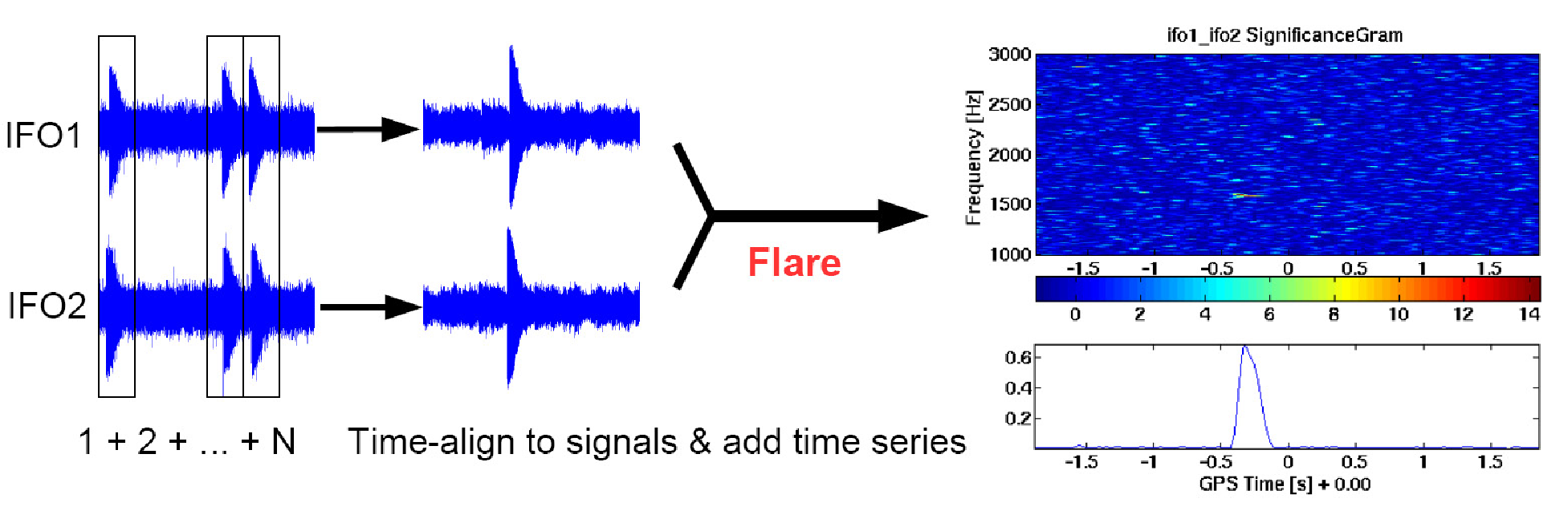
9.2.2 P-Stack incarnation
The P-Stack pipeline combines burst events in the frequency domain. Except for the addition of the frequency-domain stacking layer the P-Stack pipeline is the same as the Flare pipeline.
For each of burst events a trigger time is determined. Each of timeseries containing those triggers is processed with the Flare pipeline, up to the clustering algorithm, exactly as in an individual SGR burst search. Antenna factors are applied at this time. The result is time-frequency significance tilings. The significance tilings are then aligned to the trigger time and added together. The combined significance tiling is then fed through the Flare pipeline clustering algorithm with a fixed fraction of tiles to include in the clustering (e.g. 0.1%). A fixed fraction of tiles is used instead of a fixed loudness threshold value because the variance of the tile loudness distribution at a given frequency increases with . (In fact, clustering on a fixed fraction of tiles may be the better choice for the individual burst search as well: computer memory use is predictable even when large instrumental glitches are encountered.)
As will be described below, the P-Stack pipeline has the advantage of being relatively insensitive to timing inaccuracies or differences in waveform from burst to burst, but it has less sensitivity than the T-Stack pipeline for the (possibly unrealistic) precisely-known timing case, with deterministic waveforms.
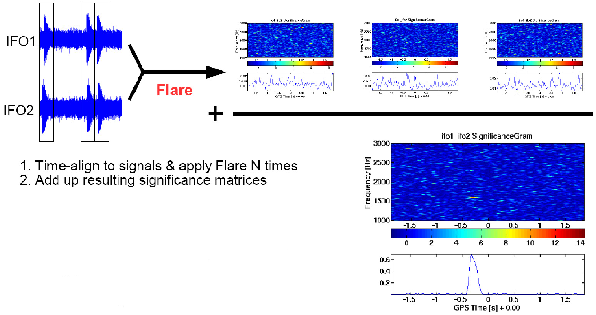
9.2.3 Loudest event upper limits
As in the individual SGR search, in the absence of a detection we still estimate loudest event upper limits [105] on gravitational wave root-sum-squared strain incident at the detector, and gravitational wave energy emitted isotropically from the source assuming a nominal source distance.
The procedure for estimating loudest event upper limits in the individual burst search is detailed in Section 5.6. In brief, the upper limit is computed in a frequentist framework following the commonly used procedure of injecting simulated signals in the background data and recovering them using the search pipeline (see for example [37, 248]). An analysis event is associated with each injected simulation, and compared to the loudest on-source analysis event. The gravitational wave strain or isotropic energy at e.g. 90% detection efficiency is the strain or isotropic energy at which 90% of injected simulations have associated events louder than the loudest on-source event.
We can follow the same procedure for the multiple burst search. The only difference is the need to measure the or of a compound injection, instead of a simple (single) injection.
9.2.4 Sensitivity dependence on
The matched filter amplitude signal-to-noise ratio (SNR) is defined in the frequency domain as [36]
| (9.1) |
where is the Fourier transform of the signal time series and is the noise power spectral density. Here, the numerator is the square root of the power in the signal. In white noise with zero mean, , a constant. Since the standard deviation of white noise goes as the square root of and the amplitude of identical stacked signals goes as , we expect the SNR of the optimal T-Stack algorithm for the recovery of identical signals from noise to go as .
While the T-Stack pipeline stacks amplitude, the P-Stack pipeline stacks power. The background tiles in the power tiling at each individual frequency bin can be modeled as Gamma-distributed noise, for which the variance also goes as , so we expect the power signal-to-noise ratio to increase as . Since the amplitude goes as the square root of the power, we expect the P-Stack amplitude sensitivity to increase as .
We tested these predictions by injecting stacked 1590 Hz 200 ms ringdowns into white noise with . We then constructed efficiency curves in the usual manner, determining the injection at 50% and 90% detection efficiency. Each efficiency curve was constructed using 20 amplitude scaling factors and 20 trials at each amplitude (see Section 5.6.6). These are bare-bone statistics, but they turned out to be effective at characterizing the Stack-a-flare pipelines. An example efficiency curve is shown in Figure 9.3.
We then fit the 50% and 90% detection efficiency level results as functions of to a two-parameter power law of the form . The results for both the T-Stack and P-Stack pipelines are shown in Figure 9.4. The fit for the T-Stack pipeline gives a sensitivity dependence in amplitude at both detection efficiency levels of nearly , confirming our prediction. This corresponds to an improvement in energy of a factor of . The fit for the P-Stack pipeline gives a sensitivity dependence in amplitude at both detection efficiency levels of nearly , confirming our prediction. This corresponds to an improvement in energy of a factor of .


We repeated the experiment for 100 ms duration 100–1000 Hz band-limited WNBs. In this case, we expected the coherent T-Stack pipeline to underperform the the P-Stack pipeline on these independently-generated stochastic incoherent signals. As expected, we found that the T-Stack pipeline shows no improvement as increases, while the P-Stack pipeline show the same sensitivity dependence seen in the coherent ringdown case. The results are shown in Figure 9.5; they illustrate the relative model-independence of the P-Stack pipeline.


9.2.5 Sensitivity dependence on timing errors
The T-Stack pipeline attains optimal sensitivity gains with increasing because it performs a phase coherent addition of signals. We have shown that the P-Stack pipeline attains its energy sensitivity performance even in the case of stacked signals that are not coherent such as independently-generated white noise bursts.
In the case of identical signals such as ringdowns, an error in the relative times between stacked signals will cause breakdown of phase coherence. For a constant timing error which is small relative to the duration of one ringdown cycle the coherence breakdown will increase with frequency. Therefore we expect the T-Stack pipeline to be more sensitive to timing errors than the P-Stack pipeline.
To begin quantifying this effect we performed a Monte Carlo with a simulated burst series roughly modeled after the SGR 1900+14 storm of 2006 March 29, with simulated 1590 Hz ms ringdown signals of equal amplitude corresponding to each of the 18 largest bursts in the storm. Timing errors were randomly chosen for each ringdown from a normal distribution with s, and were applied as a timing shift (“wiggle”) to the given ringdown. Results from a search with wiggles are then compared to the identical search with no wiggles. A s distribution was chosen for the first tests because the BAT light curve time bin size for the SGR 1900+14 storm is 100 s, which might approximate the relative timing error between bursts in the storm.
In the T-Stack case the timing degradation is approximately a factor of 1.7. In the P-Stack case no degradation was observed in this preliminary low-statistics Monte Carlo. This preliminary test implies that if timing error cannot be reduced below 100 s the P-Stack pipeline may perform better than the T-Stack pipeline for a multiple burst SGR 1900+14 storm search.


We further quantified this effect with additional Monte Carlo simulations, using a simulated burst series with equal-amplitude ringdowns, and allowing the timing error to range. We performed the Monte Carlo with two ringdown types, 1090 Hz ms and 2590 Hz ms circularly polarized ringdowns, corresponding to the low and high frequency ranges in the signal parameter space. Timing errors were randomly chosen for each ringdown from a normal distribution with ranging from 10 s to 100 ms, and were applied as a timing shift to the given ringdown. We also included the perfect timing case (no wiggle). The tests were performed with both the T-Stack and P-Stack pipelines.
As before, each efficiency curve was constructed using 20 amplitude scaling factors and 20 trials at each amplitude. These low statistics efficiency curves turned out to be adequate for characterizing the Stack-a-flare pipelines. An example efficiency curve for the timing precision Monte Carlos is shown in Figure 9.7.

The results are displayed in Figure 9.8 (1090 Hz ringdowns) and Figure 9.9 (2590 Hz ringdowns) at both the 50% and 90% detection efficiencies. As expected, the P-Stack method is independent of timing error, up until large timing errors on the order of the signal duration. The T-Stack pipeline, on the other hand, shows a pronounced dependence on timing error, which is more pronounced in the case of high frequency simulations. Each plot shows data for both T-Stack and P-Stack pipelines, and finds the equal-sensitivity timing error (P-Stack and T-Stack curve intersection point) using polynomial fits.
For the T-Stack pipeline to be effective at 1090 Hz, apparently, timing error must be s at 1-. For the T-Stack pipeline to be effective at 2590 Hz, timing error must be s at 1-. For the case shown, the T-Stack pipeline is a factor of about 1.5 more sensitivity than the P-Stack pipeline, with no or small timing errors. These precision requirements are close to the actual precision available from a continuous BAT light curve, as in the case of a storm event (Section 9.3.1).


9.2.6 Optimal use of the pipelines
We summarize the implications from characterizing the two Stack-a-flare incarnations, T-Stack and P-Stack. We envision four possible types of stacked SGR searches:
- 1.
High frequency (1000–3000 Hz) searches for ringdown burst emission, for single SGR storm events (ringdown upper limits);
- 2.
Low frequency (100–1000 Hz) searches for stochastic burst emission, for single SGR storm events (band- and time-limited WNB upper limits);
- 3.
High frequency (1000–3000 Hz) searches for ringdown burst emission, for isolated, time-separated SGR bursts (ringdown upper limits);
- 4.
Low frequency (100–1000 Hz) searches for stochastic burst emission, for isolated, time-separated SGR bursts (band- and time-limited WNB upper limits).
We have found that the P-Stack pipeline can be used effectively in any of these cases, with an energy sensitivity gain over the individual burst search of approximately . The T-Stack pipeline shows an energy sensitivity improvement of approximately , but only if the target signal is deterministic, and only if the relative timing between SGR gravitational wave burst events can be known to high precision, 100 s at 1090 Hz and 50 s at 2590 Hz or if gravitational wave data streams are time shifted relative to each other at vastly increased computational expense and additional code complexity. The T-Stack pipeline might be practical only in the first case.
9.3 SGR 1900+14 storm mock search
9.3.1 BAT light curve for the SGR 1900+14 storm
Data from the BAT detector on the Swift satellite are publicly available. In Figure 9.14, we show the storm light curve with 100 s bins. The red crosses mark burst peak heights and time locations. Times of intermediate flares were assigned at the center of the steep rising edge. Times of common bursts were assigned to the brightest bin. Figure 9.15 shows a detail of the light curve. The two major types of bursts are clearly visible: longer duration intermediate flares, and shorter duration common bursts.
It may be possible to fit the rising edges of the peaks in the light curve and perhaps obtain relative timing precision of better than a bin resolution. Even so, as we have discussed the model-dependent nature of the T-Stack method brings other disadvantages. For example, if the rise timescales determined by the fit are not the same, we would face a decision about which part of the rising edge to use when lining up stacked time series.
9.3.2 Results
The Stack-a-flare pipeline was implemented to run on either real LIGO data or simulated data. In this section we present the results of runs with the P-Stack pipeline simulating a search for gravitational waves associated with the 2006 March 29 SGR 1900+14 storm, using simulated data. At the time of the storm, all three LIGO detectors were taking science-quality data. Simulated data modeled from real data from the two LIGO 4 km detectors were created from white noise by matching power spectra with LIGO data in the frequency domain. Therefore, the sensitivity estimates should be close to upper limit estimates from real data. Although no attempt has been made to model correlations in time and frequency (e.g. glitches) which do occur in the real data, we expect agreement with results from real data to be better than 10 % on average. In fact, comparison between the mock search amplitude sensitivity estimates and closed box amplitude upper limits (presented in Table 9.2 in Section 9.4 before adding uncertainties shows average agreement to better than 1%, validating the simulated data.
For this mock search, we consider two stacking scenarios. The first scenario was an unweighted stack of the 11 bursts in the storm with the largest fluences. A histogram of integrated counts under each burst in the light curve, a measure approximately proportional to fluence, shows a clear separation between these 11 bright bursts and the rest of the set (see Figure 9.10). The second stacking scenario was the fluence-weighted scenario, which included 77 bursts in the storm light curve (all but the weakest, which would not contribute significantly). In the fluence-weighted scenario, we assume that gravitational wave emission energy is proportional to fluence, so the compound simulations are weighted to the square root of the fluence measure, and then normalized so that the total is the same as the total of the unweighted case. Then the significance tilings are weighted according to the fluence measure before being stacked.

In Figure 9.11 we show example cumulative histograms showing false alarm rates versus analysis event loudness for the background and the stacked on-source region. There are three such plots for each scenario, one per search band. Since the stacked livetime is 4 s here, the loudest on-source event occurs once per 4 s, and is plotted at a y-value of 0.25 Hz. We can estimate the FAR of this loudest on-source analysis from the background.

Table 9.1 shows sensitivity estimates, at 90% detection efficiency, for the flat scenario and the fluence-weighted scenario. Sensitivity estimates with are also shown for comparison; when the Stack-a-flare pipeline reduces to the individual burst search pipeline (Flare pipeline). Superscripts in Table 9.1 give a systematic error and uncertainties at 90% confidence. The first and second superscripts account for systematic error and statistical uncertainty in amplitude and phase of the detector calibrations, estimated via Monte Carlo simulations, respectively. The third is a statistical uncertainty arising from using a finite number of injected simulations, estimated with the bootstrap method using 200 ensembles [112]. The systematic error and the quadrature sum of the statistical uncertainties are added to the final upper limit estimates. We also present the sensitivity estimates (with uncertainties folded in) in Figures 9.12 and 9.13.


9.4 SGR 1900+14 storm closed box search
We have repeated the search described in the Section 9.3, but with real LIGO data instead of simulated LIGO-like data. This “closed box” search, done in preparation for “opening the box,” avoids analysis of the actual on-source region by adding 400 s to the electromagnetic trigger time. In other respects is identical to an actual search. The results are presented in Table 9.2. The 1% average agreement of amplitude results between the closed box and simulated data runs mentioned in the previous section indicates that the search does not strongly depend on glitchiness in the real LIGO data. Because of the close agreement, we do not show closed box figures corresponding to Figures 9.12 and 9.13.
The results in Table 9.2, while using real LIGO data, had not been reviewed by the LIGO Scientific Collaboration at the time of writing. Therefore, that table does not reflect the scientific opinion of the LSC.
9.5 Conclusion and future plans
We have presented a method for searching for gravitational waves associated with multiple SGR bursts that extends the individual SGR burst search presented in Chapter 8 and [225]. We have characterized both the T-Stack and the P-Stack incarnations of the pipeline, demonstrating sensitivity dependence on stacking number and uncertainty in relative timing between bursts. The P-Stack pipeline is robust to timing errors, and we have used it to estimate search sensitivities for a mock SGR 1900+14 storm multiple SGR search, using simulated data modeled after real LIGO data.
In the near future, we plan to perform the actual multiple burst search for gravitational waves associated with the SGR 1900+14 storm using real LIGO data. The real search will be very similar to the mock search in simulated data presented here, although we may choose to explore different or additional stacking scenarios. We are also considering a multiple SGR burst search on isolated bursts spanning months or years. The Advanced LIGO detectors promise an improvement in by more than a factor of 10 over S5, corresponding to an improvement in energy sensitivity by more than a factor of 100. We hope to continue improving this search method, and to use it to perform a searches using Advanced LIGO data.


| Flat | Fluence-weighted | |||||||||||
|---|---|---|---|---|---|---|---|---|---|---|---|---|
| Simulation type | ] | [erg] | ] | [erg] | ] | [erg] | ||||||
| WNB 11ms 100-200 Hz | 3.2 | 1.3 | 0.34 | |||||||||
| WNB 100ms 100-200 Hz | 3.0 | 1.4 | 0.39 | |||||||||
| WNB 11ms 100-1000 Hz | 6.3 | 3.8 | 0.89 | |||||||||
| WNB 100ms 100-1000 Hz | 6.2 | 4.3 | 0.98 | |||||||||
| RDC 200ms 1090 Hz | 9.1 | 4.8 | 1.1 | |||||||||
| RDC 200ms 1590 Hz | 14 | 7.1 | 1.5 | |||||||||
| RDC 200ms 2090 Hz | 19 | 8.2 | 2.2 | |||||||||
| RDC 200ms 2590 Hz | 22 | 11 | 2.4 | |||||||||
| RDL 200ms 1090 Hz | 18 | 10 | 2.7 | |||||||||
| RDL 200ms 1590 Hz | 25 | 14 | 3.3 | |||||||||
| RDL 200ms 2090 Hz | 37 | 17 | 4.8 | |||||||||
| RDL 200ms 2590 Hz | 47 | 23 | 4.7 | |||||||||
| N=1 | N=11 Flat | Fluence-weighted | ||||||||||
|---|---|---|---|---|---|---|---|---|---|---|---|---|
| Simulation type | ] | [erg] | ] | [erg] | ] | [erg] | ||||||
| WNB 11ms 100-200 Hz | 2.7 | 1.4 | 0.32 | |||||||||
| WNB 100ms 100-200 Hz | 2.8 | 1.5 | 0.32 | |||||||||
| WNB 11ms 100-1000 Hz | 5.4 | 3.2 | 0.80 | |||||||||
| WNB 100ms 100-1000 Hz | 5.1 | 4.0 | 0.92 | |||||||||
| RDC 200ms 1090 Hz | 11 | 4.7 | 1.2 | |||||||||
| RDC 200ms 1590 Hz | 14 | 7.5 | 1.7 | |||||||||
| RDC 200ms 2090 Hz | 20 | 9.0 | 2.4 | |||||||||
| RDC 200ms 2590 Hz | 20 | 11 | 2.8 | |||||||||
| RDL 200ms 1090 Hz | 19 | 8.9 | 2.0 | |||||||||
| RDL 200ms 1590 Hz | 29 | 12 | 4.1 | |||||||||
| RDL 200ms 2090 Hz | 45 | 18 | 5.1 | |||||||||
| RDL 200ms 2590 Hz | 50 | 18 | 5.6 | |||||||||
Chapter 10 Conclusion
10.1 Summary
We have described work done preparing photon calibrators for use in LIGO detectors. We have described the discovery of a significant discrepancy between calibration via photon calibrators and the coil calibration, which led to an improved understanding of LIGO detector calibration. We have described how the photon calibrators were used to discover a significant error in the detector timing calibration.
We have described the Flare pipeline, a simple but powerful tool for performing externally triggered gravitational wave searches. Though we have focused on SGR bursts in this work, the Flare pipeline is a general tool which could be used effectively in searches with other astrophysical targets. We have described work done characterizing and validating the pipeline, including analysis of GRB 070201 and comparisons to two other major LSC burst pipelines, and the LSC CBC matched filter pipeline. These are the first comparisons between coherent burst pipelines and matched filter CBC pipelines of which we are aware.
We have described a search for gravitational waves associated with the SGR 1806–20 giant flare and 214 SGR bursts in the first year of LIGO’s fifth science run [225]. The loudest events from the on-source regions analyzed are consistent with no detection. Twelve strain and twelve upper limits were set for each on-source region at 90% detection efficiency, one for each of twelve simulated signal types.
We have described a method for a powerful follow-up search which stacks individual SGR bursts in order to increase the chances for a first gravitational wave detection and significantly improve upper limits in a reasonably model-independent way.
10.2 Discussion of individual SGR burst search
Two searches for gravitational waves associated with SGR events had been published before we published our work; neither claimed detection. The AURIGA collaboration searched for gravitational wave bursts associated with the SGR 1806 giant flare in the band 850–950 Hz with damping time 100 ms, setting upper limits on the gravitational wave energy of erg [249]. The LIGO collaboration also published on the same giant flare, targeting times and frequencies of the quasi-periodic oscillations in the flare’s x-ray tail as well as other frequencies in the detector’s band, setting upper limits on gravitational wave energy as low as erg for quasi-periodic signals lasting tens of seconds [201].
In addition to the giant flare from SGR 1806–20, the search described in Chapter 8 covers 214 smaller flares which occurred during the LIGO S5 data run, when the LIGO amplitude noise was typically the value at the time of the giant flare. This was the first search sensitive to the -modes, which are usually considered the most efficient gravitational wave emitters [19]; we also searched the entire frequency band of best detector sensitivity. We have done this with unprecedentedly sensitive gravitational wave detectors, and an unprecedentedly sensitive triggered burst analysis pipeline. Not surprisingly our upper limits on gravitational wave strain amplitude were the best published to date for a short-duration gravitational wave burst search. Our upper limits on gravitational wave emission energy (Figure 8.12) overlap the range of electromagnetic energies – erg seen in SGR giant flares [126, 127] and more than one third are below the erg maximum gravitational wave energy predicted in some theoretical models [21]. Our best upper limits on are within the theoretically predicted range implied in [21].
10.3 Future work
Three new analyses are planned for the near future. First, we plan to analyze individual SGR bursts in the remainder of the S5 LIGO science run and the Virgo VSR1 science run using the Flare pipeline. Second, we plan to analyze individual SGR bursts from the newly-discovered SGR 0501+4516, which may be an order of magnitude closer to Earth than SGR 1900+14 and SGR 1806–20, using Astrowatch data from the LIGO H2 detector which was taken after the end of S5. These projects should both be straightforward, as the method is already completely implemented and reviewed. Finally, we have already begun a Stack-a-flare search for gravitational waves associated with the S5 SGR 1900+14 storm, and we expect to finish the analysis and publish the results in 2009.
As existing detectors become increasingly sensitive and new detectors in the global network come online, the prospects for detecting gravitational waves from SGRs improve. We plan to make scientific statements about gravitational waves from SGRs using data from two upcoming science runs. The enhanced LIGO detectors will double the amplitude sensitivity of S5, giving an improvement in energy sensitivity and therefore of a factor of four or more. A sixth LIGO science run (S6) with the enhanced detectors is scheduled to begin in mid-2009. Further in the future, the Advanced LIGO detectors promise an improvement in by more than a factor of 10 over S5, corresponding to an improvement in energy sensitivity (and therefore ) by more than a factor of 100.
The methods described here could usefully analyze SGR activity in future science runs. However, we will continue to search for better methods. For example, the Flare pipeline could be redesigned with the capacity to use more than two detectors. Also, the T-Stack prototype exhibits energy sensitivity gains that scale with the first power of in sandbox conditions; we would like to find a way to actualize those gains in real Stack-a-flare searches, which currently gain sensitivity as .
In conclusion, SGRs are promising sources for a first gravitational wave detection. Our analysis tools have proven to be valuable additions to the collaboration’s data analysis battery. Our work has ensured that externally triggered searches on SGR bursts will continue to be a significant part of the LSC’s science output as the detectors continue to improve.
References
- [1] A. Einstein. Die Grundlage der allgemeinen Relativitätstheorie. Annalen der Physik, 49:769–822, 1916.
- [2] R. A. Hulse and J. H. Taylor. Discovery of a pulsar in a binary system. Astrophysical Journal Letters, 195:L51–L53, January 1975.
- [3] J. H. Taylor, Jr., L. A. Fowler, and P. M. McCulloch. Measurements of general relativistic effects in the binary pulsar PSR 1913+16. Nature, 277:437, 1979.
- [4] J. H. Taylor and J. M. Weisberg. A new test of general relativity - Gravitational radiation and the binary pulsar PSR 1913+16. ApJ, 253:908–920, February 1982.
- [5] J. H. Taylor, Jr. Binary pulsars and relativistic gravity. Reviews of Modern Physics, 66:711–719, July 1994.
- [6] Clifford M. Will. The confrontation between general relativity and experiment. Living Reviews in Relativity, 9(3), 2006.
- [7] J. M. Weisberg and J. H. Taylor. The Relativistic Binary Pulsar B1913+16: Thirty Years of Observations and Analysis. In F. A. Rasio and I. H. Stairs, editors, Binary Radio Pulsars, volume 328 of Astronomical Society of the Pacific Conference Series, pages 25–+, July 2005.
- [8] B. Abbott et al. LIGO: The Laser Interferometer Gravitational-Wave Observatory. ArXiv e-prints, November 2007.
- [9] http://www.ligo.caltech.edu/advLIGO/.
- [10] http://www.ligo.caltech.edu/.
- [11] http://www.ligo.caltech.edu/.
- [12] http://www.virgo.infn.it/.
- [13] http://tamago.mtk.nao.ac.jp/.
- [14] http://www.icrr.u-tokyo.ac.jp/gr/gre.html.
- [15] http://lisa.nasa.gov/.
- [16] http://www.lisa.aei-hannover.de/.
- [17] C. Thompson and R. C. Duncan. The soft gamma repeaters as very strongly magnetized neutron stars - I. Radiative mechanism for outbursts. MNRAS, 275:255–300, July 1995.
- [18] S. J. Schwartz et al. The Gamma-Ray Giant Flare from SGR 1806–20: Evidence of Crustal Cracking via Initial Timescales. ApJ Lett., 627:L129–L132, July 2005.
- [19] N. Andersson and K. D. Kokkotas. Towards gravitational wave asteroseismology. MNRAS, 299:1059–1068, October 1998.
- [20] J. A. de Freitas Pacheco. Do soft gamma repeaters emit gravitational waves? Astronomy and Astrophysics, 336:397–401, August 1998.
- [21] K. Ioka. Magnetic deformation of magnetars for the giant flares of the soft gamma-ray repeaters. MNRAS, 327:639–662, October 2001.
- [22] N. Andersson. TOPICAL REVIEW: Gravitational waves from instabilities in relativistic stars. Class. Quant. Grav., 20:105–+, April 2003.
- [23] J. E. Horvath. Energetics of the Superflare from SGR1806–20 and a Possible Associated Gravitational Wave Burst. Modern Physics Lett. A, 20:2799–2804, 2005.
- [24] L. Ju, D. G. Blair, and C. Zhao. Detection of gravitational waves. Reports of Progress in Physics, 63:1317–1427, 2000.
- [25] E. Coccia, V. Fafone, G. Frossati, J. A. Lobo, and J. A. Ortega. A hollow sphere as a detector of gravitational radiation. Physical Review D, 57:2051, 1998.
- [26] B. F. Schutz. A First Course in General Relativity. Cambridge, UK: Cambridge University Press, February 1985.
- [27] S. M. Carroll. Spacetime and geometry. An introduction to general relativity. San Francisco, CA, USA: Addison Wesley, 2004.
- [28] C. W. Misner, K. S. Thorne, and J. A. Wheeler. Gravitation. San Francisco: W.H. Freeman and Co., 1973.
- [29] D. Sigg. Gravitational waves. In Proceedings of TASI, 98, Boulder, CO, 1998. LIGO-P980007-00-D.
- [30] L. Matone, P. Raffai, S. Marka, R. Grossman, P. Kalmus, Z. Marka, J. Rollins, and V. Sannibale. Benefits of Artificially Generated Gravity Gradients for Interferometric Gravitational-Wave Detectors. ArXiv General Relativity and Quantum Cosmology e-prints, January 2007.
- [31] K. S. Thorne. Gravitational radiation. In S. W. Hawking and W Israel, editors, 300 Years of Gravitation, page 417. Cambridge University Press, Cambridge, 1987.
- [32] LIGO Scientific Collaboration and K. Hurley. Implications for the Origin of GRB 070201 from LIGO Observations. ApJ, 681:1419–1430, July 2008.
- [33] C. D. Ott, A. Burrows, E. Livne, and R. Walder. Gravitational Waves from Axisymmetric, Rotating Stellar Core Collapse. ApJ, 600:834–864, January 2004.
- [34] H. Dimmelmeier, J. A. Font, and E. Müller. Relativistic simulations of rotational core collapse II. Collapse dynamics and gravitational radiation. A&A, 393:523–542, October 2002.
- [35] T. Zwerger and E. Mueller. Dynamics and gravitational wave signature of axisymmetric rotational core collapse. A&A, 320:209–227, April 1997.
- [36] B. Abbott et al. Analysis of ligo data for gravitational waves from binary neutron stars. Phys. Rev. D, 69(12):122001, Jun 2004.
- [37] B. Abbott et al. Search for gravitational waves from galactic and extra-galactic binary neutron stars. Phys. Rev. D, 72(8):082001, 2005.
- [38] B. Abbott et al. Search for gravitational waves from primordial black hole binary coalescences in the galactic halo. Phys. Rev. D, 72(8):082002, 2005.
- [39] B. Abbott et al. Joint ligo and tama300 search for gravitational waves from inspiralling neutron star binaries. Phys. Rev. D, 73(10):102002, 2006.
- [40] B. Abbott et al. Search for gravitational waves from binary black hole inspirals in ligo data. Phys. Rev. D, 73(6):062001, 2006.
- [41] B. Abbott et al. Search for gravitational waves from binary inspirals in s3 and s4 ligo data. Phys. Rev. D, 77(6):062002, 2008.
- [42] B. Abbott et al. Search of s3 ligo data for gravitational wave signals from spinning black hole and neutron star binary inspirals. 2007.
- [43] C. Cutler, T. A. Apostolatos, L. Bildsten, L. S. Finn, E. E. Flanagan, D. Kennefick, D. M. Markovic, A. Ori, E. Poisson, and G. J. Sussman. The last three minutes - Issues in gravitational-wave measurements of coalescing compact binaries. Phys. Rev. Lett., 70:2984–2987, May 1993.
- [44] T. A. Apostolatos. Search templates for gravitational waves from precessing, inspiraling binaries. Phys. Rev. D, 52:605–620, July 1995.
- [45] L. Bildsten and C. Cutler. Tidal interactions of inspiraling compact binaries. ApJ, 400:175–180, November 1992.
- [46] L. Blanchet, B. R. Iyer, C. M. Will, and A. G. Wiseman. Gravitational waveforms from inspiralling compact binaries to second post-Newtonian order. Class. Quant. Grav., 13:575–584, April 1996.
- [47] S. Droz, D. J. Knapp, E. Poisson, and B. J. Owen. Gravitational waves from inspiraling compact binaries: Validity of the stationary-phase approximation to the Fourier transform. Phys. Rev. D, 59(12):124016–+, June 1999.
- [48] L. Blanchet. Gravitational Radiation from Post-Newtonian Sources and Inspiralling Compact Binaries. Living Reviews in Relativity, 9:4–+, June 2006.
- [49] Alessandra Buonanno, Yanbei Chen, Yi Pan, and Michele Vallisneri. Quasiphysical family of gravity-wave templates for precessing binaries of spinning compact objects: Application to double-spin precessing binaries. Phys. Rev. D, 70(10):104003, Nov 2004.
- [50] V. Kalogera, C. Kim, D. R. Lorimer, M. Burgay, N. D’Amico, A. Possenti, R. N. Manchester, A. G. Lyne, B. C. Joshi, M. A. McLaughlin, M. Kramer, J. M. Sarkissian, and F. Camilo. The Cosmic Coalescence Rates for Double Neutron Star Binaries. ApJ Lett., 601:L179–L182, February 2004.
- [51] Lev R. Yungelson Konstantin A. Postnov. The evolution of compact binary star systems. Living Reviews in Relativity, 9(6), 2006.
- [52] LIGO Scientific Collaboration. Best Strain Sensitivities for the LIGO interferometers. LIGO Internal Note G060009-02, June 2006.
- [53] B. Abbott et al. Beating the spin-down limit on gravitational wave emission from the Crab pulsar. ArXiv e-prints, 805, May 2008.
- [54] B. Abbott et al. Setting upper limits on the strength of periodic gravitational waves from PSR J1939+2134 using the first science data from the GEO 600 and LIGO detectors. Phys. Rev. D, 69(8):082004–+, April 2004.
- [55] S. Babak, J. G. Baker, M. J. Benacquista, N. J. Cornish, J. Crowder, S. L. Larson, E. Plagnol, E. K. Porter, M. Vallisneri, A. Vecchio, K. Arnaud, L. Barack, A. Błaut, C. Cutler, S. Fairhurst, J. Gair, X. Gong, I. Harry, D. Khurana, A. Królak, I. Mandel, R. Prix, B. S. Sathyaprakash, P. Savov, Y. Shang, M. Trias, J. Veitch, Y. Wang, L. Wen, and J. T. Whelan. The Mock LISA Data Challenges: from Challenge 1B to Challenge 3. ArXiv e-prints, 806, June 2008.
- [56] Peter L Bender and Dieter Hils. Confusion noise level due to galactic and extragalactic binaries. Class. Quant. Grav., 14(6):1439–1444, 1997.
- [57] B. Abbott et al. Upper limits on a stochastic background of gravitational waves. Phys. Rev. Lett., 95(22):221101, 2005.
- [58] R. A. Battye and E. P. S. Shellard. Primordial gravitational waves : a probe of the early universe. ArXiv Astrophysics e-prints, April 1996.
- [59] Peter Fritschel, Rolf Bork, Gabriela González, Nergis Mavalvala, Dale Ouimette, Haisheng Rong, Daniel Sigg, and Michael Zucker. Readout and control of a power-recycled interferometric gravitational-wave antenna. Appl. Opt., 40(28):4988–4998, 2001.
- [60] D. Abramovici et al. Science, 256:325, 1992.
- [61] http://www.ligo.caltech.edu/docs/G/G060009-03/.
- [62] R.L. Savage, P.J. King, and S.U. Seel. A highly stabilized 10-watt Nd:YAG laser for the laser interferometer gravitational-wave observatory (LIGO). Laser Phys., 8:679, 1998.
- [63] R.W.P. Drever et al. Laser phase and frequency stabilization using an optical resonator. Appl. Phys. B: Photophys. Laser Chem., 31:97–105, 1983.
- [64] A. Ruldiger et al. A mode selector to suppress fluctuations in laser beam geometry. Optica Acta, 28:641, 1981.
- [65] Brian J. Meers. Recycling in laser-interferometric gravitational-wave detectors. Phys. Rev. D, 38(8):2317–2326, Oct 1988.
- [66] H. B. Callen and T. A. Welton. Irreversibility and generalized noise.
- [67] LIGO Scientific Collaboration: B. Abbott et al. Detector Description and Performance for the First Coincidence Observations between LIGO and GEO. Nucl. Instrum. Methods A, 517, 2004.
- [68] B. Barish and R. Weiss. LIGO and the Detection of Gravitational Waves. Phys. Today, 52, October 1999.
- [69] D. Sigg. Strain Calibration in LIGO. LIGO Internal Note T970101-B-D, 2003.
- [70] A. Dietz et al. Calibration of the LIGO detectors for S4. LIGO Internal Note T050262-00-D, 2006.
- [71] R. Adhikari, G. González, M. Landry, B. O’Reilly, and the LIGO Scientific Collaboration. Calibration of the LIGO detectors for the First LIGO Science Run. Class. Quant. Grav., 20:903–+, September 2003.
- [72] G. González, M. Landry, B. O’Reilly, and H. Radkins. Calibration of the LIGO detectors for S2. LIGO Internal Note T040060-01-D, 2004.
- [73] G. González, M. Landry, B. O’Reilly, and X. Siemens. Calibration of the LIGO detectors for S3. LIGO Internal Note T050059-01-D, 2005.
- [74] R. Adhikari et al. Input test mass (ITM) absolute calibrations: fringe counting, fringe fitting, and sign toggling methods. LIGO Internal Note T020141-01-D, 2002.
- [75] X. Siemens et al. Making h(t) for LIGO. Class. Quant. Grav., 21:S1723, May 2004.
- [76] http://lancelot.mit.edu/cadonati/S5/DQkleinFullS5-v3/Summary.html.
- [77] P. R. Saulson. Fundamentals of interferometric gravitational wave detectors. Singapore: World Scientific Publishers, 1994.
- [78] W. G. Anderson, P. R. Brady, J. D. Creighton, and É. É. Flanagan. Excess power statistic for detection of burst sources of gravitational radiation. Phys. Rev. D, 63(4):042003–+, February 2001.
- [79] Landry M. Enhanced LIGO Status - PAC 24 Meeting @ LIGO Hanford Observatory, June 24-25, 2008. LIGO Internal Note G080387-00-D, 2008.
- [80] Fritschel P. and Coyne D. Technical Status of Advanced LIGO. LIGO Internal Note G080391-00, 2008.
- [81] Y. Aso. Active Vibration Isolation for a Laser Interferometric Gravitational Wave Detector using a Suspension Point Interferometer. PhD thesis, University of Tokyo, 2008.
- [82] J. Bruursema. Calibration of the LIGO Interferometer Using the Recoil of Photons. LIGO Internal Note G030513-00-D, 2003.
- [83] E. Goetz. Commissioning of the Photon Calibrators. LIGO Internal Note T040196-00-D, 2004.
- [84] E. Goetz, P. Kalmus, and R. Savage. Commissioning of the Photon Calibrators. LIGO Internal Note T070026-00-W, 2007.
- [85] D. A. Clubley, G. P. Newton, K. D. Skeldon, and J. Hough. Calibration of the Glasgow 10 m prototype laser interferometric gravitational wave detector using photon pressure. Physics Letters A, 283:85–88, May 2001.
- [86] K. Mossavi, M. Hewitson, S. Hild, F. Seifert, U. Weiland, J. R. Smith, H. Lück, H. Grote, B. Willke, and K. Danzmann. A photon pressure calibrator for the GEO 600 gravitational wave detector. Physics Letters A, 353:1–3, April 2006.
- [87] P. Kalmus. State of the Photon Calibrators. LIGO Internal Note G05433-00-I, 2005. Talk presented at 2005 August LSC meeting at Hanford.
- [88] code written by M. Evans.
- [89] Personal communication with D. Froman, Scientech Inc.
- [90] http://www.ligo-wa.caltech.edu/gds/.
- [91] P. Kalmus. Discrepancy Between Photon Calibration and Official Calibration. LIGO Internal Note G060687-00-I, 2006. Talk presented at 2006 May 15 Commissioning Meeting.
- [92] W. Winkler, K. Danzmann, A. Rüdiger, and R. Schilling. Heating by optical absorption and the performance of interferometric gravitational-wave detectors. Phys. Rev. A, 44:7022–7036, December 1991.
- [93] S. Rao. Mirror Thermal Noise in Interferometric GravitationalWave Detectors. PhD thesis, California Institute of Technology, 2003.
- [94] E. Goetz and P. Kalmus. State of the Photon Calibrators. LIGO Internal Note G060686-00-I, 2006. Talk presented at August 2006 LSC meeting at LSU.
- [95] E. Goetz, P. Kalmus, and R. Savage. Status of the Photon Calibrators. LIGO Internal Note G060647-00-I, 2006. Talk presented at 2006 December 11 Commissioning Telecon.
- [96] S. Hild, M. Brinkmann, K. Danzmann, H. Grote, M. Hewitson, J. Hough, H. Lück, I. Martin, K. Mossavi, N. Rainer, S. Reid, J. R. Smith, K. Strain, M. Weinert, P. Willems, B. Willke, and W. Winkler. Photon-pressure-induced test mass deformation in gravitational-wave detectors. Class. Quant. Grav., 24:5681–5688, November 2007.
- [97] National Institute of Standards and Technology. Report of calibration (42110CA/42111CA). LIGO Internal Note T070245-00-W, 2008.
- [98] E. Goetz and R. Savage. Investigation of discrepancies between Photon calibrator, VCO and Official (coil) calibration techniques. LIGO Internal Note G080216-00-Z, 2008. Talk presented at March 2008 LSC-VIRGO meeting.
- [99] Y. Aso et al. Accurate measurement of the time delay in the response of the LIGO gravitational wave detectors. 2008. submitted to CQG.
- [100] N. Smith and D. Sigg. LIGO Internal Note T080039-00-D, 2008.
- [101] M. Smith and P. Willems. Advanced LIGO Photon Calibrator Conceptual Design. LIGO Internal Note T070167-01-D, 2007.
- [102] P. Kalmus et al. Search method for unmodeled transient gravitational waves associated with SGR Flares. Class. Quant. Grav., 24:S659–S669, October 2007.
- [103] É. É. Flanagan and S. A. Hughes. Measuring gravitational waves from binary black hole coalescences. I. Signal to noise for inspiral, merger, and ringdown. Phys. Rev. D, 57:4535–4565, April 1998.
- [104] É. É. Flanagan and S. A. Hughes. Measuring gravitational waves from binary black hole coalescences. II. The waves’ information and its extraction, with and without templates. Phys. Rev. D, 57:4566–4587, April 1998.
- [105] P. R. Brady, J. D. E. Creighton, and A. G. Wiseman. Upper limits on gravitational-wave signals based on loudest events. Class. Quant. Grav., 21:S1775, May 2004.
- [106] B. Abbott et al. Search for gravitational-wave bursts in ligo data from the fourth science run. Class. Quant. Grav., 24(22):5343–5369, 2007.
- [107] R. Hamming. Digital Filters. Dover Publications, New York, 1998.
- [108] R. Khan and S. Chatterji. Enhancing the capabilities of LIGO time-frequency plane searches through clustering. in progress, 2007.
- [109] K Thorne. https://gravity.psu.edu/psurg/sims/burstmdc/index.html.
- [110] S. Shapiro and S. Teukolsky. Black Holes, White Dwarfs, and Neutron Stars. Wiley, New York, 1983.
- [111]
P Sutton.
http://www.ligo.caltech.edu/˜psutton/protected/
xpipeline/xpipeline.html. - [112] B. Efron. Bootstrap methods: another look at the jackknife. Ann. Statist., 7:1–26, 1979.
- [113] http://lhocds.ligo-wa.caltech.edu/scirun/S4/HardwareInjection/.
- [114] http://lhocds.ligo-wa.caltech.edu/scirun/S5/HardwareInjection/.
- [115] LIGO Scientific Collaboration. Best Strain Sensitivities for the LIGO Interferometers, Early S5 Performance. LIGO Internal Note G060010, January 2006.
- [116] B. Abbott et al. Search for gravitational-wave bursts in LIGO data from the fourth science run. ArXiv e-prints, 704, April 2007.
- [117] K. Hurley et al. Where is SGR 1806–20? ApJ Lett., 523:L37–L40, September 1999.
- [118] S. Golentskii et al. IPN localization of very intense short GRB 070201. GRB Coordinates Network, 6088, 2008.
- [119] S. Klimenko. Coherent WaveBurst. LIGO note T060282-00-Z, 2006.
- [120] S. Klimenko, I. Yakushin, A. Mercer, and G. Mitselmakher. A coherent method for detection of gravitational wave bursts. Class. Quant. Grav., 25(11):114029–+, June 2008.
- [121] S. Klimenko, S. Mohanty, Malik Rakhmanov, and G. Mitselmakher. Constraint likelihood analysis for a network of gravitational wave detectors. Phys. Rev. D, 72:122002, 2005.
- [122] S. Klimenko. http://www.lsc-group.phys.uwm.edu/cgi-bin/Analysis/Waveburst/S4/wat.
- [123] S. Klimenko, I. Yakushin, and G. Mitselmakher. WaveBurst: S5 version. LIGO note T060112-00-Z, 2006.
- [124] Shourov Chatterji, Albert Lazzarini, Leo Stein, Patrick J. Sutton, Antony Searle, and Massimo Tinto. Coherent network analysis technique for discriminating gravitational-wave bursts from instrumental noise. Phys. Rev. D, 74(8):082005, 2006.
- [125] F. Beauville et al. A comparison of methods for gravitational wave burst searches from LIGO and Virgo. Class. Quant. Grav., 25:045002, 2008.
- [126] K. Hurley et al. An exceptionally bright flare from SGR 1806–20 and the origins of short-duration -ray bursts. Nature, 434:1098–1103, April 2005.
- [127] D. M. Palmer et al. A giant -ray flare from the magnetar SGR 1806 - 20. Nature, 434:1107–1109, April 2005.
- [128] T. Terasawa, Y. T. Tanaka, Y. Takei, N. Kawai, A. Yoshida, K. Nomoto, I. Yoshikawa, Y. Saito, Y. Kasaba, T. Takashima, T. Mukai, H. Noda, T. Murakami, K. Watanabe, Y. Muraki, T. Yokoyama, and M. Hoshino. Repeated injections of energy in the first 600ms of the giant flare of SGR1806 - 20. Nature, 434:1110–1111, April 2005.
- [129] E. Smith, J. Swank, C. Markwardt, Y. Rephaeli, D. Gruber, M. Persic, and R. Rothschild. SGR1806–20: RXTE-PCA observation of the 041227 super-flare. GRB Coordinates Network, 2927, 2005.
- [130] E. Mazets, S. Golenetskii, R. Aptekar, D. Frederiks, V. Pal’Shin, and T. Cline. The giant outburst from SGR 1806–20. GRB Coordinates Network, 2922, 2004.
- [131] J. Borkowski, D. Gotz, S. Mereghetti, N. Mowlavi, S. Shaw, and M. Turler. Giant flare from SGR 1806–20 detected by INTEGRAL. GRB Coordinates Network, 2920, 2004.
- [132] S. Boggs, K. Hurley, D. M. Smith, R. P. Lin, G. Hurford, W. Hajdas, and C. Wigger. SGR 1806–20, RHESSI observations of the 041227 giant flare. GRB Coordinates Network, 2936, 2005.
- [133] D. Palmer et al. SGR1806–20: Swift-BAT observation of the 041227 super-flare. GRB Coordinates Network, 2925, 2004.
- [134] U. S. Inan, N. G. Lehtinen, R. C. Moore, K. Hurley, S. Boggs, D. M. Smith, and G. J. Fishman. Massive disturbance of the daytime lower ionosphere by the giant -ray flare from magnetar SGR 1806-20. Geophys. Res. Lett., 34:8103–+, April 2007.
- [135] S. Golenetskii, R. Aptekar, E. Mazets, V. Pal’Shin, D. Frederiks, and T. Cline. Detection of the SGR 1806–20 giant outburst back-scattered by the. GRB Coordinates Network, 2923, 2004.
- [136] S. Mereghetti, D. Götz, I. F. Mirabel, and K. Hurley. INTEGRAL discovery of persistent hard X-ray emission from the Soft Gamma-ray Repeater SGR 1806–20. Astronomy and Astrophysics, 433:L9–L12, April 2005.
- [137] K. Hurley, T. Cline, I. Mitrofanov, S. Charyshnikov, V. Grinkov, A. Kozyrev, M. Litvak, A. Sanin, W. Boynton, C. Fellows, K. Harshman, C. Shinohara, and R. Starr. IPN localization of giant flare from SGR1806–20. GRB Coordinates Network, 2921, 2004.
- [138] S. Mereghetti. The strongest cosmic magnets: Soft Gamma-ray Repeaters and Anomalous X-ray Pulsars. A&A Rev., 15:225–287, 2008.
- [139] P. M. Woods and C. Thompson. Soft gamma repeaters and anomalous x-ray pulsars: Magnetar candidates. In W. G. H. Lewin and M. van der Klis, editors, Compact Stellar X-Ray Sources. Cambridge Univ. Press, Cambridge, 2004.
- [140] S. T. Holland et al. GRB 080822: Swift detection of a short burst. GRB Coordinates Network, 8112, 2008.
- [141] C. Kouveliotou, S. Dieters, T. Strohmayer, J. van Paradijs, G. J. Fishman, C. A. Meegan, K. Hurley, J. Kommers, I. Smith, D. Frail, and T. Murakami. An X-ray pulsar with a superstrong magnetic field in the soft gamma-ray repeater SGR 1806–20. Nature, 393:235–237, 1998.
- [142] S. Barthelmy et al. New Soft Gamma Repeater 0501+4516 was GRB 080822. GRB Coordinates Network, 8113, 2008.
- [143] D. Palmer and S. Barthelmy. Third event from SGR 0501+4516. GRB Coordinates Network, 8115, 2008.
- [144] B. M. Gaensler and S. Chatterjee. SGR 0501+4516: Proximity to supernova remnant HB9. GRB Coordinates Network, 8149, 2008.
- [145] D. A. Leahy and B. Aschenbach. ROSAT X-ray observations of the supernova remnant HB 9. A&A, 293:853–858, January 1995.
- [146] E. P. Mazets et al. Observations of a flaring X-ray pulsar in Dorado. Nature, 282:587–589, December 1979.
- [147] K. Hurley et al. A giant periodic flare from the soft gamma-ray repeater SGR 1900+14. Nature, 397:41–43, 1999.
- [148] P. A. Evans and J. P. Osborne. Enhanced Swift-XRT position of SGR 0501+4516. GRB Coordinates Network, 8148, 2008.
- [149] P. M. Woods , E. Gogus, and C. Kouveliotou. SGR 0501+4516: Spin Down Rate and Inferred Dipole Magnetic Field. GRB Coordinates Network, 8166, 2008.
- [150] D. L. Kaplan, S. R. Kulkarni, M. H. van Kerkwijk, R. E. Rothschild, R. L. Lingenfelter, D. Marsden, R. Danner, and T. Murakami. Hubble Space Telescope Observations of SGR 0526-66: New Constraints on Accretion and Magnetar Models. ApJ, 556:399–407, July 2001.
- [151] S. R. Kulkarni, D. L. Kaplan, H. L. Marshall, D. A. Frail, T. Murakami, and D. Yonetoku. The Quiescent Counterpart of the Soft Gamma-Ray Repeater SGR 0526-66. ApJ, 585:948–954, March 2003.
- [152] S. Klose, A. A. Henden, U. Geppert, J. Greiner, H. H. Guetter, D. H. Hartmann, C. Kouveliotou, C. B. Luginbuhl, B. Stecklum, and F. J. Vrba. A Near-Infrared Survey of the N49 Region around the Soft Gamma Repeater SGR 0526-66. ApJ Lett., 609:L13–L16, July 2004.
- [153] S. Wachter, S. K. Patel, C. Kouveliotou, P. Bouchet, F. Özel, A. F. Tennant, P. M. Woods, K. Hurley, W. Becker, and P. Slane. Precise Localization of the Soft Gamma Repeater SGR 1627-41 and the Anomalous X-Ray Pulsar AXP 1E1841-045 with Chandra. ApJ, 615:887–896, November 2004.
- [154] D. L. Kaplan, D. W. Fox, S. R. Kulkarni, E. V. Gotthelf, G. Vasisht, and D. A. Frail. Precise Chandra Localization of the Soft Gamma-Ray Repeater SGR 1806–20. ApJ, 564:935–940, January 2002.
- [155] S. Corbel and S. S. Eikenberry. The connection between W31, SGR 1806–20, and LBV 1806–20: Distance, extinction, and structure. A&A, 419:191–201, May 2004.
- [156] Y. Fuchs, F. Mirabel, S. Chaty, A. Claret, C. J. Cesarsky, and D. A. Cesarsky. ISO observations of the environment of the soft gamma-ray repeater SGR 1806-20. A&A, 350:891–899, October 1999.
- [157] D. A. Frail, S. R. Kulkarni, and J. S. Bloom. An outburst of relativistic particles from the soft gamma-ray repeater SGR 1900+14. Nature, 398:127, 1999.
- [158] D. L. Kaplan, S. R. Kulkarni, D. A. Frail, and M. H. van Kerkwijk. Deep Radio, Optical, and Infrared Observations of SGR 1900+14. ApJ, 566:378–386, February 2002.
- [159] F. J. Vrba, C. B. Luginbuhl, A. A. Henden, H. H. Guetter, and D. H. Hartmann. Search for photometric variability in the vicinity of SGR 1900+14 and discovery of a high-mass cluster. In R. M. Kippen, R. S. Mallozzi, and G. J. Fishman, editors, Gamma-ray Bursts, 5th Huntsville Symposium, volume 526 of American Institute of Physics Conference Series, pages 809–813, September 2000.
- [160] R. L. Aptekar, D. D. Frederiks, S. V. Golenetskii, V. N. Il’inskii, E. P. Mazets, V. D. Pal’shin, P. S. Butterworth, and T. L. Cline. Konus Catalog of Soft Gamma Repeater Activity: 1978 to 2000. ApJ, Supplement, 137:227–277, December 2001.
- [161] E. Göğüş, C. Kouveliotou, P. M. Woods, C. Thompson, R. C. Duncan, and M. S. Briggs. Temporal and Spectral Characteristics of Short Bursts from the Soft Gamma Repeaters 1806-20 and 1900+14. ApJ, 558:228–236, September 2001.
- [162] C. Kouveliotou, J. P. Norris, T. L. Cline, B. R. Dennis, U. D. Desai, L. E. Orwig, E. E. Fenimore, R. W. Klebesadel, J. G. Laros, J.-L. Atteia, M. Boer, K. Hurley, M. Neil, G. Vedrenne, A. V. Kuznetsov, R. A. Sunyaev, and O. V. Terekhov. SMM hard X-ray observations of the soft gamma-ray repeater 1806-20. ApJ Lett., 322:L21–L25, November 1987.
- [163] B. Cheng, R. I. Epstein, R. A. Guyer, and A. C. Young. Earthquake-like behaviour of soft -ray repeaters. Nature, 382:518–520, August 1996.
- [164] E. GöğüŞ , P. M. Woods, C. Kouveliotou, J. van Paradijs, M. S. Briggs, R. C. Duncan, and C. Thompson. Statistical Properties of SGR 1900+14 Bursts. ApJ Lett., 526:L93–L96, December 1999.
- [165] P. M. Woods. The dynamic behavior of soft gamma repeaters. Advances in Space Research, 33:630–637, 2004.
- [166] J.-F. Olive, K. Hurley, J.-P. Dezalay, J.-L. Atteia, C. Barraud, N. Butler, G. B. Crew, J. Doty, G. Ricker, R. Vanderspek, D. Q. Lamb, N. Kawai, A. Yoshida, Y. Shirasaki, T. Sakamoto, T. Tamagawa, K. Torii, M. Matsuoka, E. E. Fenimore, M. Galassi, T. Tavenner, T. Q. Donaghy, and C. Graziani. FREGATE observation of a strong burst from SGR1900+14. In G. R. Ricker and R. K. Vanderspek, editors, Gamma-Ray Burst and Afterglow Astronomy 2001: A Workshop Celebrating the First Year of the HETE Mission, volume 662 of American Institute of Physics Conference Series, pages 82–87, April 2003.
- [167] T. L. Cline. A review of the 1979 March 5 transient. In R. E. Lingenfelter, H. S. Hudson, and D. M. Worall, editors, Gamma Ray Transients and Related Astrophysical Phenomena, volume 77 of American Institute of Physics Conference Series, pages 17–33, 1982.
- [168] T. L. Cline, U. D. Desai, B. J. Teegarden, W. D. Evans, R. W. Klebesadel, J. G. Laros, C. Barat, K. Hurley, M. Niel, and M. C. Weisskopf. Precise source location of the anomalous 1979 March 5 gamma-ray transient. ApJ Lett., 255:L45–L48, April 1982.
- [169] S. V. Golenetskii, V. N. Ilinskii, and E. P. Mazets. Recurrent bursts in GBS0526 - 66, the source of the 5 March 1979 gamma-ray burst. Nature, 307:41–43, January 1984.
- [170] E. E. Fenimore, W. D. Evans, R. W. Klebesadel, J. G. Laros, and J. Terrell. Spectral evolution of the 5 March 1979 gamma burst. Nature, 289:42–+, January 1981.
- [171] U. S. Inan, N. G. Lehtinen, S. J. Lev-Tov, M. P. Johnson, T. F. Bell, and K. Hurley. Ionization of the lower ionosphere by -rays from a magnetar: Detection of a low energy (3-10 keV) component. Geophys. Res. Lett., 26:3357–3360, November 1999.
- [172] P. M. Woods, C. Kouveliotou, J. van Paradijs, M. H. Finger, C. Thompson, R. C. Duncan, K. Hurley, T. Strohmayer, J. Swank, and T. Murakami. Variable Spin-Down in the Soft Gamma Repeater SGR 1900+14 and Correlations with Burst Activity. ApJ Lett., 524:L55–L58, October 1999.
- [173] N. Rea, G. L. Israel, S. Mereghetti, A. Tiengo, S. Zane, R. Turolla, and L. Stella. Magnetars’ Giant Flares: the Case of SGR 1806 20. Chinese Journal of Astronomy and Astrophysics Supplement, 6(1):010000–158, December 2006.
- [174] G. L. Israel, T. Belloni, L. Stella, Y. Rephaeli, D. E. Gruber, P. Casella, S. Dall’Osso, N. Rea, M. Persic, and R. E. Rothschild. The Discovery of Rapid X-Ray Oscillations in the Tail of the SGR 1806–20 Hyperflare. ApJ Lett., 628:L53–L56, July 2005.
- [175] B. M. Gaensler, C. Kouveliotou, J. D. Gelfand, G. B. Taylor, D. Eichler, R. A. M. J. Wijers, J. Granot, E. Ramirez-Ruiz, Y. E. Lyubarsky, R. W. Hunstead, D. Campbell-Wilson, A. J. van der Horst, M. A. McLaughlin, R. P. Fender, M. A. Garrett, K. J. Newton-McGee, D. M. Palmer, N. Gehrels, and P. M. Woods. An expanding radio nebula produced by a giant flare from the magnetar SGR 1806–20. Nature, 434:1104–1106, April 2005.
- [176] S. E. Boggs, A. Zoglauer, E. Bellm, K. Hurley, R. P. Lin, D. M. Smith, C. Wigger, and W. Hajdas. The Giant Flare of December 27, 2004 from SGR 1806–20. ArXiv e-prints, November 2006.
- [177] A. Watts and T. Strohmayer. Neutron starquake shakes RHESSI. January 2006.
- [178] T. E. Strohmayer and A. L. Watts. Discovery of Fast X-Ray Oscillations during the 1998 Giant Flare from SGR 1900+14. ApJ Lett., 632:L111–L114, October 2005.
- [179] C. Guidorzi, F. Frontera, E. Montanari, M. Feroci, L. Amati, E. Costa, and M. Orlandini. Comparative study of the two large flares from SGR1900+14 with the BeppoSAX Gamma-Ray Burst Monitor. A&A, 416:297–310, March 2004.
- [180] J.-F. Olive, K. Hurley, T. Sakamoto, J.-L. Atteia, G. Crew, G. Ricker, G. Pizzichini, C. Barraud, and N. Kawai. Time-resolved X-Ray Spectral Modeling of an Intermediate Burst from SGR 1900+14 Observed by HETE-2 FREGATE and WXM. ApJ, 616:1148–1158, December 2004.
- [181] K. Hurley, C. Kouveliotou, P. Woods, T. Cline, P. Butterworth, E. Mazets, S. Golenetskii, and D. Frederics. Reactivation and Precise Interplanetary Network Localization of the Soft Gamma Repeater SGR 1900+14. ApJ Lett., 510:L107–L109, January 1999.
- [182] E. P. Mazets, T. L. Cline, R. L. Aptekar’, P. S. Butterworth, D. D. Frederiks, S. V. Golenetskii, V. N. Il’Inskii, and V. D. Pal’Shin. Activity of the soft gamma repeater SGR 1900 + 14 in 1998 from Konus-Wind observations: 1. Short recurrent bursts. Astronomy Letters, 25:628–634, October 1999.
- [183] G. L. Israel, P. Romano, V. Mangano, S. Dall’Osso, G. Chincarini, L. Stella, S. Campana, T. Belloni, G. Tagliaferri, A. J. Blustin, T. Sakamoto, K. Hurley, S. Zane, A. Moretti, D. Palmer, C. Guidorzi, D. N. Burrows, N. Gehrels, and H. A. Krimm. A Swift Gaze into the 2006 March 29 Burst Forest of SGR 1900+14. ApJ, 685:1114–1128, October 2008.
- [184] D. Palmer et al. Reactivation of SGR 1627-41. GRB Coordinates Network, 7777, 2008.
- [185] P.M. Woods, C. Kouveliotou, E. Gogos, K. Hurley, and J. Tomsick. RXTE Observations of Renewed Burst Activity from SGR 1627-41. Atel, 1549, 2008.
- [186] S. V. Golenetskiy, R. L. Aptekar, Y. A. Guryan, V. N. Ilinskiy, and Y. P. Mazets. Observations of gamma bursts from GBS 0526-66. JPRS Report Science Technology USSR Space, 5:54–+, November 1987.
- [187] K. Hurley. The 4.5+/-0.5 soft gamma repeaters in review. In R. M. Kippen, R. S. Mallozzi, and G. J. Fishman, editors, Gamma-ray Bursts, 5th Huntsville Symposium, volume 526 of American Institute of Physics Conference Series, pages 763–770, September 2000.
- [188] P. M. Woods, C. Kouveliotou, J. van Paradijs, K. Hurley, R. M. Kippen, M. H. Finger, M. S. Briggs, S. Dieters, and G. J. Fishman. Discovery of a New Soft Gamma Repeater, SGR 1627-41. ApJ Lett., 519:L139–L142, July 1999.
- [189] E. Gogus et al. Discovery of the Spin Period of the New Soft Gamma Repeater SGR 0501+4516. GRB Coordinates Network, 8118, 2008.
- [190] V. Mangano et al. SGR 0501+4516: Swift XRT measure of the spin period. GRB Coordinates Network, 8146, 2008.
- [191] D. Palmer. SGR 0501+4516: Decline in Activity. Atel, 1683, 2008.
- [192] G. J. Fishman et al. SGR 0501+4516: Fermi GBM (formerly GLAST Burst Monitor) observations of three exceptionally intense outbursts. GRB Coordinates Network, 8139, 2008.
- [193] T. Cline, D. D. Frederiks, S. Golenetskii, K. Hurley, C. Kouveliotou, E. Mazets, and J. van Paradijs. Observations of a Possible New Soft Gamma Repeater, SGR 1801-23. ApJ, 531:407–410, March 2000.
- [194] D. Marsden and N. E. White. Correlations between Spectral Properties and Spin-down Rate in Soft Gamma-Ray Repeaters and Anomalous X-Ray Pulsars. ApJ Lett., 551:L155–L158, April 2001.
- [195] T. Oosterbroek, A. N. Parmar, S. Mereghetti, and G. L. Israel. The two-component X-ray spectrum of the 6.4 S pulsar 1E 1048.1-5937. A&A, 334:925–930, June 1998.
- [196] P. M. Woods, C. Kouveliotou, E. Göğüş, M. H. Finger, J. Swank, D. A. Smith, K. Hurley, and C. Thompson. Evidence for a Sudden Magnetic Field Reconfiguration in Soft Gamma Repeater 1900+14. ApJ, 552:748–755, May 2001.
- [197] P. M. Woods, C. Kouveliotou, E. Göğüş, M. H. Finger, J. Swank, C. B. Markwardt, K. Hurley, and M. van der Klis. Large Torque Variations in Two Soft Gamma Repeaters. ApJ, 576:381–390, September 2002.
- [198] P. M. Woods, C. Kouveliotou, M. H. Finger, E. Göğüş, C. A. Wilson, S. K. Patel, K. Hurley, and J. H. Swank. The Prelude to and Aftermath of the Giant Flare of 2004 December 27: Persistent and Pulsed X-Ray Properties of SGR 1806–20 from 1993 to 2005. ApJ, 654:470–486, January 2007.
- [199] A. L. Watts and T. E. Strohmayer. Detection with RHESSI of High-Frequency X-Ray Oscillations in the Tail of the 2004 Hyperflare from SGR 1806–20. ApJ Lett., 637:L117–L120, February 2006.
- [200] C. Barat, R. I. Hayles, K. Hurley, M. Niel, G. Vedrenne, U. Desai, V. G. Kurt, V. M. Zenchenko, and I. V. Estulin. Fine time structure in the 1979 March 5 gamma ray burst. A&A, 126:400–402, October 1983.
- [201] B. Abbott et al. Search for gravitational wave radiation associated with the pulsating tail of the SGR 1806–20 hyperflare of 27 December 2004 using LIGO. Phys. Rev. D, 76:062003, 2007.
- [202] T. E. Strohmayer and A. L. Watts. The 2004 Hyperflare from SGR 1806–20: Further Evidence for Global Torsional Vibrations. ArXiv Astrophysics e-prints, August 2006.
- [203] W. D. Evans, R. W. Klebesadel, J. G. Laros, T. L. Cline, U. D. Desai, B. J. Teegarden, G. Pizzichini, K. Hurley, M. Niel, and G. Vedrenne. Location of the gamma-ray transient event of 1979 March 5. ApJ Lett., 237:L7–L9, April 1980.
- [204] K. Hurley, P. Li, C. Kouveliotou, T. Murakami, M. Ando, T. Strohmayer, J. van Paradijs, F. Vrba, C. Luginbuhl, A. Yoshida, and I. Smith. ASCA Discovery of an X-Ray Pulsar in the Error Box of SGR 1900+14. ApJ Lett., 510:L111–L114, January 1999.
- [205] S. R. Kulkarni, D. A. Frail, N. E. Kassim, T. Murakami, and G. Vasisht. The Radio Nebula of the Soft Gamma-Ray Repeater 1806–20. Nature, 368:129–+, March 1994.
- [206] S. R. Kulkarni, K. Matthews, G. Neugebauer, I. N. Reid, M. H. van Kerkwijk, and G. Vasisht. Optical and infrared observations of SGR 1806-20. ApJ Lett., 440:L61–L64, February 1995.
- [207] M. H. van Kerkwijk, S. R. Kulkarni, K. Matthews, and G. Neugebauer. A luminous companion to SGR 1806-20. ApJ Lett., 444:L33–L35, May 1995.
- [208] S. S. Eikenberry, K. Matthews, J. L. LaVine, M. A. Garske, D. Hu, M. A. Jackson, S. G. Patel, D. J. Barry, M. R. Colonno, J. R. Houck, J. C. Wilson, S. Corbel, and J. D. Smith. Infrared Observations of the Candidate LBV 1806-20 and Nearby Cluster Stars1,. ApJ, 616:506–518, November 2004.
- [209] S. S. Eikenberry, M. A. Garske, D. Hu, M. A. Jackson, S. G. Patel, D. J. Barry, M. R. Colonno, and J. R. Houck. Possible Infrared Counterparts to the Soft Gamma-Ray Repeater SGR 1806-20. ApJ Lett., 563:L133–L137, December 2001.
- [210] P. B. Cameron, P. Chandra, A. Ray, S. R. Kulkarni, D. A. Frail, M. H. Wieringa, E. Nakar, E. S. Phinney, A. Miyazaki, M. Tsuboi, S. Okumura, N. Kawai, K. M. Menten, and F. Bertoldi. Detection of a radio counterpart to the 27 December 2004 giant flare from SGR 1806–20. Nature, 434:1112–1115, April 2005.
- [211] S. Corbel, P. Wallyn, T. M. Dame, P. Durouchoux, W. A. Mahoney, O. Vilhu, and J. E. Grindlay. The Distance of the Soft Gamma Repeater SGR 1806-20. ApJ, 478:624–+, March 1997.
- [212] G. Vasisht, S. R. Kulkarni, D. A. Frail, and J. Greiner. Supernova remnant candidates for the soft gamma-ray repeater 1900+14. ApJ Lett., 431:L35–L38, August 1994.
- [213] D. K. Milne. A new catalogue of galactic SNRs corrected for distance from the galactic plane. Australian Journal of Physics, 32:83–92, March 1979.
- [214] P. M. W. Kalberla, W. B. Burton, D. Hartmann, E. M. Arnal, E. Bajaja, R. Morras, and W. G. L. Pöppel. The Leiden/Argentine/Bonn (LAB) Survey of Galactic HI. Final data release of the combined LDS and IAR surveys with improved stray-radiation corrections. A&A, 440:775–782, September 2005.
- [215] F. J. Vrba, C. B. Luginbuhl, K. C. Hurley, P. Li, S. R. Kulkarni, M. H. van Kerkwijk, D. H. Hartmann, L. E. Campusano, M. J. Graham, R. G. Clowes, C. Kouveliotou, R. Probst, I. Gatley, M. Merrill, R. Joyce, R. Mendez, I. Smith, and A. Schultz. The Double Infrared Source toward the Soft Gamma-Ray Repeater SGR 1900+14. ApJ, 468:225–+, September 1996.
- [216] R. C. Duncan and C. Thompson. Formation of very strongly magnetized neutron stars - Implications for gamma-ray bursts. ApJ Lett., 392:L9–L13, June 1992.
- [217] S. R. Kulkarni and D. A. Frail. Identification of a supernova remnant coincident with the soft gamma-ray repeater SGR1806–20. Nature, 365:33–35, September 1993.
- [218] R. C. Duncan. Physics in ultra-strong magnetic fields. In R. M. Kippen, R. S. Mallozzi, and G. J. Fishman, editors, Gamma-ray Bursts, 5th Huntsville Symposium, volume 526 of American Institute of Physics Conference Series, pages 830–841, September 2000.
- [219] F. C. Michel. Theory of Neutron Star Magnetospheres. Univ. Chigaco Press, Chicago, 1991.
- [220] C. Kouveliotou, T. Strohmayer, K. Hurley, J. van Paradijs, M. H. Finger, S. Dieters, P. Woods, C. Thompson, and R. C. Duncan. Discovery of a Magnetar Associated with the Soft Gamma Repeater SGR 1900+14. ApJ Lett., 510:L115–L118, January 1999.
- [221] C. Thompson and R. C. Duncan. The Soft Gamma Repeaters as Very Strongly Magnetized Neutron Stars. II. Quiescent Neutrino, X-Ray, and Alfven Wave Emission. ApJ, 473:322–+, December 1996.
- [222] http://solomon.as.utexas.edu/duncan/magnetar.html.
- [223] D. M. Palmer. SGR 1806-20 Is a Set of Independent Relaxation Systems. ApJ Lett., 512:L113–L116, February 1999.
- [224] C. Thompson, R. C. Duncan, P. M. Woods, C. Kouveliotou, M. H. Finger, and J. van Paradijs. Physical Mechanisms for the Variable Spin-down and Light Curve of SGR 1900+14. ApJ, 543:340–350, November 2000.
- [225] B. Abbott et al. Search for gravitational-wave bursts from soft gamma repeaters. Phys. Rev. Lett., 101(21):211102, 2008.
- [226] O. Benhar, V. Ferrari, and L. Gualtieri. Gravitational wave asteroseismology reexamined. Phys. Rev. D, 70(12):124015–+, December 2004.
- [227] B. L. Schumaker and K. S. Thorne. Torsional oscillations of neutron stars. MNRAS, 203:457–489, May 1983.
- [228] http://ssl.berkeley.edu/ipn3.
- [229] Personal communication with K. Hurley.
- [230] http://gcn.gsfc.nasa.gov.
- [231] http://hessi.ssl.berkeley.edu/.
- [232] http://swift.gsfc.nasa.gov/docs/swift/swiftsc.html.
- [233] http://www-spof.gsfc.nasa.gov/istp/wind/.
- [234] http://integral.esac.esa.int/.
- [235] http://www.isas.jaxa.jp/e/enterp/missions/suzaku/index.shtml.
- [236] S. Golenetskii et al. Konus-Wind observation of the recent SGR 1900+14 activity. GRB Coordinates Network, 4946, 2006.
- [237] K. Hurley et al. IPN triangulation of GRB060806 (long, exceptionally bright). GRB Coordinates Network, 5416, 2006.
- [238] K. Hurley et al. GRB060806 = SGR1806–20. GRB Coordinates Network, 5419, 2006.
- [239] Personal communication with D. Frederiks.
- [240] S. Golenetskii et al. GRB060806 is similar to previous activity of SGR1806–20. GRB Coordinates Network, 5426, 2006.
- [241] C. Thompson and R. C. Duncan. The Giant Flare of 1998 August 27 from SGR 1900+14. II. Radiative Mechanism and Physical Constraints on the Source. ApJ, 561:980–1005, November 2001.
- [242] F. Raab. "Astrowatch" at LIGO Hanford Observatory. LIGO Internal Note G050122, 2005.
- [243] Personal communication with M. Landry.
- [244] P. Kalmus. mattapps Flare package, CVS tag “open4-v3”, 2008. input/calibration/H1response_788218239.txt.
- [245] 2008 May 16 communication from B. O’Reilly to the LSC.
- [246] Personal communication with B. O’Reilly.
- [247] Calibration Team. S5 V3 Error Budget. LIGO Internal Note (document number not available), 2008.
- [248] B. Abbott et al. Search for gravitational waves associated with 39 gamma-ray bursts using data from the second, third, and fourth ligo runs. Phys. Rev. D, 77(6):062004, 2008.
- [249] L. Baggio, M. Bignotto, M. Bonaldi, M. Cerdonio, L. Conti, M. De Rosa, P. Falferi, P. Fortini, M. Inguscio, N. Liguori, F. Marin, R. Mezzena, A. Mion, A. Ortolan, G. A. Prodi, S. Poggi, F. Salemi, G. Soranzo, L. Taffarello, G. Vedovato, A. Vinante, S. Vitale, and J. P. Zendri AURIGA Collaboration. Erratum: Upper Limits on Gravitational-Wave Emission in Association with the 27 Dec 2004 Giant Flare of SGR 1806–20. Phys. Rev. Lett., 95(13):139903, 2005.
- [250] K. Cannon, P. Kalmus, and B. Owen. SGR burst analysis review. LIGO Internal Note T080256-00-Z, 2008.
- [251] G. G. Lichti, R. Georgii, A. von Kienlin, V. Schönfelder, C. Wunderer, H.-J. Jung, and K. Hurley. The -Ray Burst-Detection System of SPI. In M. L. McConnell and J. M. Ryan, editors, American Institute of Physics Conference Series, pages 722–+, 2000.
- [252] Personal communication with D. Smith.
- [253] Personal communication with G. Lichti.
Chapter A Glossary
| Term | Definition |
|---|---|
| ACIGA | Australian Consortium for Interferometric Gravitational Astronomy |
| ADC | Analog to Digital Converter |
| AEG | Analysis Event Generator |
| AIGO | Australian Interferometric Gravitational Observatory |
| AIGRC | Australian International Gravitational Research Centre |
| AXP | Anomalous X-ray Pulsar |
| BAT | Burst Alert Telescope, detector on Swift satellite |
| BATSE | detector on NASA’s Compton Gamma-Ray Observatory satellite |
| BBH | Binary Black Hole |
| BH | Black Hole |
| BNS | Binary Neutron Star |
| BP | Bandpass |
| BS | Beam Splitter |
| CBC | Compact Binary Coalescence |
| Chandra | Chandra X-ray observatory satellite |
| cWB | Coherent WaveBurst analysis pipeline |
| D1 | Detector 1 |
| D2 | Detector 2 |
| DARM | Differential Arm |
| DAC | Digital to Analog Converter |
| DAQ | Data Acquisition |
| DCC | Document Control Center |
| DFT | Discrete Fourier Transform |
| DMT | Data Monitor Tool |
| DQ | Data Quality |
| EndX | X-arm ETM on an interferometer |
| EndY | Y-arm ETM on an interferometer |
| EOS | Equation of State |
| ETM | End Test Mass |
| GCN | GRB Coordinate Network |
| GR | General Theory of Relativity |
| GRB | Gamma Ray Burst |
| GW | Gravitational Wave |
| H1 | LIGO Hanford Observatory 4 km detector |
| H1X | H1 detector X-arm end station |
| H1Y | H1 detector Y-arm end station |
| H2 | LIGO Hanford Observatory 2 km detector |
| H2X | H2 detector X-arm end station |
| H2Y | H2 detector Y-arm end station |
| HR | Highly Reflective (optical coating) |
| HW | Hardware |
| IBAS | INTEGRAL Burst Alert System |
| IFO | interferometer |
| IPN | InterPlanetary Network |
| ITM | Input Test Mass |
| Konus | Gamma-ray detector on Wind satellite |
| L1 | LIGO Livingston Observatory 4 km detector |
| L1X | L1 detector X-arm end station |
| L1Y | L1 detector Y-arm end station |
| LAL | LIGO Algorithm Library |
| LBV | Luminous Blue Variable |
| LCGT | Large Scale Cryogenic Gravitational Wave Telescope |
| LHO | LIGO Hanford Observatory |
| LIGO | Laser Interferometer Gravitational-Wave Observatory |
| LISA | Laser Interferometer Space Antenna |
| LLO | LIGO Livingston Observatory |
| LMC | Large Magellanic Cloud |
| LSC | LIGO Scientific Collaboration |
| LTF | Likelihood Time-Frequency map |
| MDC | Mock Data Challenge |
| NIST | National Institute of Standards and Technology |
| nfft | Fourier transform length in samples |
| NS | Neutron Star |
| OSEM | Optical Shadow Sensor and Electromagnetic Actuator |
| OTTB | Optically Thin Thermal Bremsstrahlung |
| overlap | Fourier transform overlap |
| pcal | photon calibrator |
| PD | Photodetector |
| PBH | Primordial Black Hole |
| PSL | Pre-Stabilized Laser |
| PSR | Pulsar |
| QPO | Quasiperiodic Oscillation |
| RD | Ringdown |
| RDL | Linear ringdown |
| RDC | Circular ringdown |
| RHESSI | Ramaty High Energy Solar Spectroscopic Imager (satellite) |
| RXTE | Rossi X-Ray Timing Explorer (satellite) |
| S5 | LIGO’s fifth science run |
| S5y1 | First year of S5 14 Nov. 2005 to 14 Nov. 2006 |
| SG | Sine-Gaussian |
| SGR | Soft Gamma Repeater |
| SNR | Signal to Noise Ratio |
| SNR | Supernova Remnant |
| SPI | Suspension Point Interferometer |
| SR | Special Theory of Relativity |
| SRD | Science Requirements Document |
| Swift | IPN satellite with BAT detector |
| TAMA | Tokyo Advanced Medium-Scale Antenna |
| TF | Time and Frequency |
| Ulysses | solar observatory satellite |
| VLA | Very Large Array |
| WAT | Wavelet Analysis Toolbox |
| Wind | IPN satellite with Konus detector |
| WNB | band- and time-lmited White Noise Burst |
| XRT | X-Ray Telescope (on Swift satellite) |
| loudness statistic |
Chapter B Technical Flare pipeline validations
Here we present additional checks of the data conditioning algorithm and time bookkeeping. The Flare pipeline underwent a formal code review performed by an LSC review committee, and some of these checks were done as part of the formal review process.
B.1 Data conditioning stage
We first look at the effect of a 64–2048 Hz bandpass filter on white noise, in the frequency domain (Figure B.1). This filter is representative of bandpass filters used in searches, which may have different pass bands. In the middle of the passband the filter gain is 1.

We next examine the effect of a representative notch filter. Figure B.2 shows periodograms of unnotched and notched simulated LIGO data (simulated data are described in Section 6.6.1.
Spectrograms showing the progression from bandpassed unnotched LIGO noise, to bandpassed notched noise, to noise after whitening via the Flare excess power algorithm described in Section 5.4.2 are shown in Figures B.3 through B.5. Several simulated large band WNBs were injected into the noise in order to qualitatively demonstrate the effect of filtering on signals.


B.2 Validation of time bookkeeping
We generate ASCII lists of analysis events for all simulation recovery and on-source regions. These lists are checked to insure that time bookkeeping is performed correctly, that is, that analysis event times are all contained in the expected region. A script produced by an LSC reviewer (K. Cannon) checks the analysis event time dumps from the pipeline and verifies that no event lies outside of the segment in which it was supposed to be found [250]. This test passes.
B.3 Comparison of Flare and LAL simulations
We produced samples of Flare pipeline simulations for comparison to simulations produced by LAL simulation code. A test program written by an LSC reviewer (K. Cannon) loads two files produced by the Flare pipeline: a raw file containing the original injection plus- and cross-polarization time series, and a post-injection dump file containing the H1 and L1 time series [250]. The test program uses LAL injection code to convert the Flare plus- and cross-polarization time series into a prediction of the H1 and L1 strains. The LAL and Flare versions of the instrument strains are dumped together into two files, one for each instrument. Figure B.6 shows the extent of the discrepancy.


B.4 Validation of simulation calculation
Comparisons between values for simulations computed by Flare and LAL agree to within a few times double-precision epsilon.
B.5 Validation of simulation calculation
Flare pipeline calculated for the injection samples described in Section B.3. These calculations were compared to reviewed LAL code. The values computed for the waveforms agree to within 0.1% with the exception of the lowest-frequency WNB waveforms, where Flare assigns an energy about 1% higher than LAL does. This is in the safe direction – Flare is either correct or computing a conservative upper limit if LAL is correct – and is small compared to other sources of uncertainty. After investigation, the source of this 1% discrepancy remains unidentified.
B.6 Validation of antenna factor calculation
The comparison in Section B.3 also provides stringent, if qualitative, validation of Flare’s antenna factor code. In addition, during the course of review we directly compared Flare and LAL and antenna factors over a mesh of 167936 combinations of sky positions, polarizations, and times. The time range spanned a UTC leap second where the correct GPS to GMST conversion should make the Earth appear to rotate backwards momentarily.
B.7 Simulation time delays in Fourier space
The comparison in Section B.3 also provides stringent, if qualitative, validation of Flare’s simulation time delay code. In addition, the Flare pipeline code for performing time delays in Fourier space on simulations has been incorporated into the BurstMDC simulations engine [109], the primary external simulations engine for the LSC Burst Working Group. The Flare pipeline code has given BurstMDC the capability of performing subsample time delays. BurstMDC has since undergone an independent review, further validating this function.
B.8 Upper limit results from Flare vs. BurstMDC simulations
In addition to comparisons with LAL, upper limits for 16 searches (2 GPS times and 8 simulations – RDC and RDL) estimated using simulations produced with Flare pipelines internal simulations engine were compared to upper limits estimated using MDCs produced by BurstMDC [109]. Average agreement was better than 2%.
B.9 Validation of events list generation
The Flare pipeline looks at on-source regions which are fed to it in the events list. Not only must Flare do this correctly (as checked in Section B.2), but the listed on-source regions must be correct as well. In addition, in order to estimate the on-source loudest event significance and upper limits correctly, the background segment list in the events list must be correct.
Creating the events list is described in Section 5.3. There are several things to check here. UTC times from the IPN list must be correctly converted to GPS times. DQ segments must be collated correctly for the on-source and background regions. For Konus-Wind events, timing must be propagated correctly from satellite crossing time to Earth crossing time.
The events list was reproduced starting from the original upstream files and using entirely independent LAL code (e.g. LAL light travel-time functions, UTC-to-GPS conversions, segment algebra functions etc.) [250]. With the exception of 1 s discrepancies in background segment times consistent with rounding fluctuations, the reproduction and original events lists are the same.
Additionally, in the course of procuring the SGR 1806–20 060806 event Konus-Wind light curve, D. Frederiks calculated the time between light crossing at the geocenter and light crossing at the satellite at 06 Aug 2006 14:23:44.12 UTC to be 5.051 s [239]. We had previously calculated it to be 5.0508 s. This provides external validation of the light crossing time propagation technique.
We further validated the calculation using a second method based on trigonometry instead of rotations.
Chapter C Propagation of light crossing times
In this appendix we describe the method for propagation of satellite light crossing times.
In the individual SGR burst search described in Chapter 8, the giant flare event time was propagated from a satellite crossing time to a crossing time at the Hanford LIGO site, while 21 of the S5y1 events times were propagated from the Konus satellite to the geocenter.
Propagation of the wavefront arrival time to the geocenter requires knowledge of the SGR sky position and knowledge of the satellite position relative to the geocenter. Propagation of the wavefront arrival time to the gravitational wave detector requires knowledge of the position of the detector on the Earth relative to the geocenter as well. Positions of the source are given in terms of right ascension and declination, and positions of satellites an locations on earth are given in terms of right-handed sky-fixed geocentered cartesian coordinates, with the Z-axis pointing north and the X-axis pointing to the vernal equinox. Converting detector latitudes and longitudes to these coordinates requires knowledge of the sidereal time of the event.
Propagation was performed via rotation matrices. The first rotation around the Z-axis causes the Y-axis to be perpendicular to the source-geocenter line, and the second rotation around the Y-axis causes the X-axis to point to the source. After these rotations are applied, we take the difference in satellite and Earth X-coordinates and divide by the speed of light to get the relative light crossing delay. Validation of this technique is described in Section B.9.
As an example, we discuss the peak time of the giant flare event in detail. GCN reports 2920 [131] and 2936 [132] assign times for the giant flare wavefront arrival time at the INTEGRAL and RHESSI satellites respectively. The RHESSI timing declares a 3 ms systematic error, while the INTEGRAL timing is considered to be accurate to within 50 ms [251]. Therefore, we use the RHESSI time for our trigger time, and the INTEGRAL time provides a cross check.
The time of the abrupt rise of the giant flare at RHESSI was 21:30:26.6376(30) UT on 2004 December 27 [252]. This agrees with the time cited in [176], 21:30:26.64, but disagrees with the time cited in the GCN report which was incorrect [252]. The light crossing time at INTEGRAL was 21:30:26:55(5) UT [253] which is consistent with the corrected RHESSI time given the locations of the satellites and source.
We find that the wavefront arrived at Hanford 5.88 ms after it arrived at the RHESSI satellite, and 81.0 ms after arrival at the INTEGRAL satellite.
Therefore, we choose to center our search at 21:30:26.643(3) UT on 2004 December 27, corresponding to the arrival of the rising edge of the giant flare at the detector. This trigger time corresponds to a GPS time of 788218239.643(3). We note that the individual burst search does not require more than 1 s precision in the external trigger times; the above determination with millisecond precision was performed before it was clear that the search was much more tolerant of timing imprecision.
Chapter D Full Table of Upper Limits for the Giant Flare and S5y1 flares
| trigger | detector | type | o.s. | ] | [erg] | ||||
|---|---|---|---|---|---|---|---|---|---|
| SGR 1806 | H1 | 0.29 | - | WNB 11ms 100-200Hz | 4 | ||||
| WNB 100ms 100-200Hz | 4 | ||||||||
| GPS 788218239.643 | WNB 11ms 100-1000Hz | 4 | |||||||
| Dec 27 2004 21:30:26.643 UTC | WNB 100ms 100-1000Hz | 4 | |||||||
| RDC 200ms 1090Hz | 4 | ||||||||
| RDC 200ms 1590Hz | 4 | ||||||||
| RDC 200ms 2090Hz | 4 | ||||||||
| RDC 200ms 2590Hz | 4 | ||||||||
| RDL 200ms 1090Hz | 4 | ||||||||
| RDL 200ms 1590Hz | 4 | ||||||||
| RDL 200ms 2090Hz | 4 | ||||||||
| RDL 200ms 2590Hz | 4 | ||||||||
| SGR 1806 | L1H1H2 | 0.63 | 0.58 | WNB 11ms 100-200Hz | 4 | ||||
| WNB 100ms 100-200Hz | 4 | ||||||||
| GPS 817466383.2 | WNB 11ms 100-1000Hz | 4 | |||||||
| Dec 01 2005 09:59:30.2 UTC | WNB 100ms 100-1000Hz | 4 | |||||||
| RDC 200ms 1090Hz | 4 | ||||||||
| RDC 200ms 1590Hz | 4 | ||||||||
| RDC 200ms 2090Hz | 4 | ||||||||
| RDC 200ms 2590Hz | 4 | ||||||||
| RDL 200ms 1090Hz | 4 | ||||||||
| RDL 200ms 1590Hz | 4 | ||||||||
| RDL 200ms 2090Hz | 4 | ||||||||
| RDL 200ms 2590Hz | 4 | ||||||||
| SGR 1806 | L1H1H2 | 0.63 | 0.64 | WNB 11ms 100-200Hz | 4 | ||||
| WNB 100ms 100-200Hz | 4 | ||||||||
| GPS 817635844.3 | WNB 11ms 100-1000Hz | 4 | |||||||
| Dec 03 2005 09:03:51.3 UTC | WNB 100ms 100-1000Hz | 4 | |||||||
| RDC 200ms 1090Hz | 4 | ||||||||
| RDC 200ms 1590Hz | 4 | ||||||||
| RDC 200ms 2090Hz | 4 | ||||||||
| RDC 200ms 2590Hz | 4 | ||||||||
| RDL 200ms 1090Hz | 4 | ||||||||
| RDL 200ms 1590Hz | 4 | ||||||||
| RDL 200ms 2090Hz | 4 | ||||||||
| RDL 200ms 2590Hz | 4 | ||||||||
| SGR 1806 | L1H1H2 | 0.56 | 0.40 | WNB 11ms 100-200Hz | 4 | ||||
| WNB 100ms 100-200Hz | 4 | ||||||||
| GPS 817645421.3 | WNB 11ms 100-1000Hz | 4 | |||||||
| Dec 03 2005 11:43:28.3 UTC | WNB 100ms 100-1000Hz | 4 | |||||||
| RDC 200ms 1090Hz | 4 | ||||||||
| RDC 200ms 1590Hz | 4 | ||||||||
| RDC 200ms 2090Hz | 4 | ||||||||
| RDC 200ms 2590Hz | 4 | ||||||||
| RDL 200ms 1090Hz | 4 | ||||||||
| RDL 200ms 1590Hz | 4 | ||||||||
| RDL 200ms 2090Hz | 4 | ||||||||
| RDL 200ms 2590Hz | 4 | ||||||||
| SGR 1806 | L1H1H2 | 0.56 | 0.39 | WNB 11ms 100-200Hz | 4 | ||||
| WNB 100ms 100-200Hz | 4 | ||||||||
| GPS 817645533.0 | WNB 11ms 100-1000Hz | 4 | |||||||
| Dec 03 2005 11:45:20.0 UTC | WNB 100ms 100-1000Hz | 4 | |||||||
| RDC 200ms 1090Hz | 4 | ||||||||
| RDC 200ms 1590Hz | 4 | ||||||||
| RDC 200ms 2090Hz | 4 | ||||||||
| RDC 200ms 2590Hz | 4 | ||||||||
| RDL 200ms 1090Hz | 4 | ||||||||
| RDL 200ms 1590Hz | 4 | ||||||||
| RDL 200ms 2090Hz | 4 | ||||||||
| RDL 200ms 2590Hz | 4 | ||||||||
| SGR 1806 | L1H1H2 | 0.46 | 0.23 | WNB 11ms 100-200Hz | 4 | ||||
| WNB 100ms 100-200Hz | 4 | ||||||||
| GPS 817736037.0 | WNB 11ms 100-1000Hz | 4 | |||||||
| Dec 04 2005 12:53:44.0 UTC | WNB 100ms 100-1000Hz | 4 | |||||||
| RDC 200ms 1090Hz | 4 | ||||||||
| RDC 200ms 1590Hz | 4 | ||||||||
| RDC 200ms 2090Hz | 4 | ||||||||
| RDC 200ms 2590Hz | 4 | ||||||||
| RDL 200ms 1090Hz | 4 | ||||||||
| RDL 200ms 1590Hz | 4 | ||||||||
| RDL 200ms 2090Hz | 4 | ||||||||
| RDL 200ms 2590Hz | 4 | ||||||||
| SGR 1806 | H1H2 | 0.21 | - | WNB 11ms 100-200Hz | 4 | ||||
| WNB 100ms 100-200Hz | 4 | ||||||||
| GPS 817748941.0 | WNB 11ms 100-1000Hz | 4 | |||||||
| Dec 04 2005 16:28:48.0 UTC | WNB 100ms 100-1000Hz | 4 | |||||||
| RDC 200ms 1090Hz | 4 | ||||||||
| RDC 200ms 1590Hz | 4 | ||||||||
| RDC 200ms 2090Hz | 4 | ||||||||
| RDC 200ms 2590Hz | 4 | ||||||||
| RDL 200ms 1090Hz | 4 | ||||||||
| RDL 200ms 1590Hz | 4 | ||||||||
| RDL 200ms 2090Hz | 4 | ||||||||
| RDL 200ms 2590Hz | 4 | ||||||||
| SGR 1806 | H1H2 | 0.28 | - | WNB 11ms 100-200Hz | 4 | ||||
| WNB 100ms 100-200Hz | 4 | ||||||||
| GPS 817939110.0 | WNB 11ms 100-1000Hz | 4 | |||||||
| Dec 06 2005 21:18:17.0 UTC | WNB 100ms 100-1000Hz | 4 | |||||||
| RDC 200ms 1090Hz | 4 | ||||||||
| RDC 200ms 1590Hz | 4 | ||||||||
| RDC 200ms 2090Hz | 4 | ||||||||
| RDC 200ms 2590Hz | 4 | ||||||||
| RDL 200ms 1090Hz | 4 | ||||||||
| RDL 200ms 1590Hz | 4 | ||||||||
| RDL 200ms 2090Hz | 4 | ||||||||
| RDL 200ms 2590Hz | 4 | ||||||||
| SGR 1806 | L1H1H2 | 0.53 | 0.68 | WNB 11ms 100-200Hz | 4 | ||||
| WNB 100ms 100-200Hz | 4 | ||||||||
| GPS 822538468.0 | WNB 11ms 100-1000Hz | 4 | |||||||
| Jan 29 2006 02:54:14.0 UTC | WNB 100ms 100-1000Hz | 4 | |||||||
| RDC 200ms 1090Hz | 4 | ||||||||
| RDC 200ms 1590Hz | 4 | ||||||||
| RDC 200ms 2090Hz | 4 | ||||||||
| RDC 200ms 2590Hz | 4 | ||||||||
| RDL 200ms 1090Hz | 4 | ||||||||
| RDL 200ms 1590Hz | 4 | ||||||||
| RDL 200ms 2090Hz | 4 | ||||||||
| RDL 200ms 2590Hz | 4 | ||||||||
| SGR 1806 | L1 | - | 0.60 | WNB 11ms 100-200Hz | 4 | ||||
| WNB 100ms 100-200Hz | 4 | ||||||||
| GPS 824272814.0 | WNB 11ms 100-1000Hz | 4 | |||||||
| Feb 18 2006 04:40:00.0 UTC | WNB 100ms 100-1000Hz | 4 | |||||||
| RDC 200ms 1090Hz | 4 | ||||||||
| RDC 200ms 1590Hz | 4 | ||||||||
| RDC 200ms 2090Hz | 4 | ||||||||
| RDC 200ms 2590Hz | 4 | ||||||||
| RDL 200ms 1090Hz | 4 | ||||||||
| RDL 200ms 1590Hz | 4 | ||||||||
| RDL 200ms 2090Hz | 4 | ||||||||
| RDL 200ms 2590Hz | 4 | ||||||||
| SGR 1900+14 | H1H2 | 0.24 | - | WNB 11ms 100-200Hz | 4 | ||||
| WNB 100ms 100-200Hz | 4 | ||||||||
| GPS 827316739.0 | WNB 11ms 100-1000Hz | 4 | |||||||
| Mar 25 2006 10:12:05.0 UTC | WNB 100ms 100-1000Hz | 4 | |||||||
| RDC 200ms 1090Hz | 4 | ||||||||
| RDC 200ms 1590Hz | 4 | ||||||||
| RDC 200ms 2090Hz | 4 | ||||||||
| RDC 200ms 2590Hz | 4 | ||||||||
| RDL 200ms 1090Hz | 4 | ||||||||
| RDL 200ms 1590Hz | 4 | ||||||||
| RDL 200ms 2090Hz | 4 | ||||||||
| RDL 200ms 2590Hz | 4 | ||||||||
| SGR 1900+14 | L1H1H2 | 0.45 | 0.31 | WNB 11ms 100-200Hz | 4 | ||||
| WNB 100ms 100-200Hz | 4 | ||||||||
| GPS 827345255.0 | WNB 11ms 100-1000Hz | 4 | |||||||
| Mar 25 2006 18:07:21.0 UTC | WNB 100ms 100-1000Hz | 4 | |||||||
| RDC 200ms 1090Hz | 4 | ||||||||
| RDC 200ms 1590Hz | 4 | ||||||||
| RDC 200ms 2090Hz | 4 | ||||||||
| RDC 200ms 2590Hz | 4 | ||||||||
| RDL 200ms 1090Hz | 4 | ||||||||
| RDL 200ms 1590Hz | 4 | ||||||||
| RDL 200ms 2090Hz | 4 | ||||||||
| RDL 200ms 2590Hz | 4 | ||||||||
| SGR 1900+14 | L1H1 | 0.35 | 0.52 | WNB 11ms 100-200Hz | 4 | ||||
| WNB 100ms 100-200Hz | 4 | ||||||||
| GPS 827364861.0 | WNB 11ms 100-1000Hz | 4 | |||||||
| Mar 25 2006 23:34:07.0 UTC | WNB 100ms 100-1000Hz | 4 | |||||||
| RDC 200ms 1090Hz | 4 | ||||||||
| RDC 200ms 1590Hz | 4 | ||||||||
| RDC 200ms 2090Hz | 4 | ||||||||
| RDC 200ms 2590Hz | 4 | ||||||||
| RDL 200ms 1090Hz | 4 | ||||||||
| RDL 200ms 1590Hz | 4 | ||||||||
| RDL 200ms 2090Hz | 4 | ||||||||
| RDL 200ms 2590Hz | 4 | ||||||||
| SGR 1900+14 | H1 | 0.43 | - | WNB 11ms 100-200Hz | 4 | ||||
| WNB 100ms 100-200Hz | 4 | ||||||||
| GPS 827369976.0 | WNB 11ms 100-1000Hz | 4 | |||||||
| Mar 26 2006 00:59:22.0 UTC | WNB 100ms 100-1000Hz | 4 | |||||||
| RDC 200ms 1090Hz | 4 | ||||||||
| RDC 200ms 1590Hz | 4 | ||||||||
| RDC 200ms 2090Hz | 4 | ||||||||
| RDC 200ms 2590Hz | 4 | ||||||||
| RDL 200ms 1090Hz | 4 | ||||||||
| RDL 200ms 1590Hz | 4 | ||||||||
| RDL 200ms 2090Hz | 4 | ||||||||
| RDL 200ms 2590Hz | 4 | ||||||||
| SGR 1900+14 | L1H1H2 | 0.55 | 0.65 | WNB 11ms 100-200Hz | 4 | ||||
| WNB 100ms 100-200Hz | 4 | ||||||||
| GPS 827415018.0 | WNB 11ms 100-1000Hz | 4 | |||||||
| Mar 26 2006 13:30:04.0 UTC | WNB 100ms 100-1000Hz | 4 | |||||||
| RDC 200ms 1090Hz | 4 | ||||||||
| RDC 200ms 1590Hz | 4 | ||||||||
| RDC 200ms 2090Hz | 4 | ||||||||
| RDC 200ms 2590Hz | 4 | ||||||||
| RDL 200ms 1090Hz | 4 | ||||||||
| RDL 200ms 1590Hz | 4 | ||||||||
| RDL 200ms 2090Hz | 4 | ||||||||
| RDL 200ms 2590Hz | 4 | ||||||||
| SGR 1900+14 | L1H1H2 | 0.52 | 0.44 | WNB 11ms 100-200Hz | 4 | ||||
| WNB 100ms 100-200Hz | 4 | ||||||||
| GPS 827427031.0 | WNB 11ms 100-1000Hz | 4 | |||||||
| Mar 26 2006 16:50:17.0 UTC | WNB 100ms 100-1000Hz | 4 | |||||||
| RDC 200ms 1090Hz | 4 | ||||||||
| RDC 200ms 1590Hz | 4 | ||||||||
| RDC 200ms 2090Hz | 4 | ||||||||
| RDC 200ms 2590Hz | 4 | ||||||||
| RDL 200ms 1090Hz | 4 | ||||||||
| RDL 200ms 1590Hz | 4 | ||||||||
| RDL 200ms 2090Hz | 4 | ||||||||
| RDL 200ms 2590Hz | 4 | ||||||||
| SGR 1900+14 | L1H1H2 | 0.43 | 0.55 | WNB 11ms 100-200Hz | 4 | ||||
| WNB 100ms 100-200Hz | 4 | ||||||||
| GPS 827542829.0 | WNB 11ms 100-1000Hz | 4 | |||||||
| Mar 28 2006 01:00:15.0 UTC | WNB 100ms 100-1000Hz | 4 | |||||||
| RDC 200ms 1090Hz | 4 | ||||||||
| RDC 200ms 1590Hz | 4 | ||||||||
| RDC 200ms 2090Hz | 4 | ||||||||
| RDC 200ms 2590Hz | 4 | ||||||||
| RDL 200ms 1090Hz | 4 | ||||||||
| RDL 200ms 1590Hz | 4 | ||||||||
| RDL 200ms 2090Hz | 4 | ||||||||
| RDL 200ms 2590Hz | 4 | ||||||||
| SGR 1900+14 | L1H1H2 | 0.47 | 0.64 | WNB 11ms 100-200Hz | 4 | ||||
| WNB 100ms 100-200Hz | 4 | ||||||||
| GPS 827582256.0 | WNB 11ms 100-1000Hz | 4 | |||||||
| Mar 28 2006 11:57:22.0 UTC | WNB 100ms 100-1000Hz | 4 | |||||||
| RDC 200ms 1090Hz | 4 | ||||||||
| RDC 200ms 1590Hz | 4 | ||||||||
| RDC 200ms 2090Hz | 4 | ||||||||
| RDC 200ms 2590Hz | 4 | ||||||||
| RDL 200ms 1090Hz | 4 | ||||||||
| RDL 200ms 1590Hz | 4 | ||||||||
| RDL 200ms 2090Hz | 4 | ||||||||
| RDL 200ms 2590Hz | 4 | ||||||||
| SGR 1900+14 | L1H1H2 | 0.47 | 0.64 | WNB 11ms 100-200Hz | 4 | ||||
| WNB 100ms 100-200Hz | 4 | ||||||||
| GPS 827582369.0 | WNB 11ms 100-1000Hz | 4 | |||||||
| Mar 28 2006 11:59:15.0 UTC | WNB 100ms 100-1000Hz | 4 | |||||||
| RDC 200ms 1090Hz | 4 | ||||||||
| RDC 200ms 1590Hz | 4 | ||||||||
| RDC 200ms 2090Hz | 4 | ||||||||
| RDC 200ms 2590Hz | 4 | ||||||||
| RDL 200ms 1090Hz | 4 | ||||||||
| RDL 200ms 1590Hz | 4 | ||||||||
| RDL 200ms 2090Hz | 4 | ||||||||
| RDL 200ms 2590Hz | 4 | ||||||||
| SGR 1900+14 | H1H2 | 0.17 | - | WNB 11ms 100-200Hz | 4 | ||||
| WNB 100ms 100-200Hz | 4 | ||||||||
| GPS 827611902.0 | WNB 11ms 100-1000Hz | 4 | |||||||
| Mar 28 2006 20:11:28.0 UTC | WNB 100ms 100-1000Hz | 4 | |||||||
| RDC 200ms 1090Hz | 4 | ||||||||
| RDC 200ms 1590Hz | 4 | ||||||||
| RDC 200ms 2090Hz | 4 | ||||||||
| RDC 200ms 2590Hz | 4 | ||||||||
| RDL 200ms 1090Hz | 4 | ||||||||
| RDL 200ms 1590Hz | 4 | ||||||||
| RDL 200ms 2090Hz | 4 | ||||||||
| RDL 200ms 2590Hz | 4 | ||||||||
| SGR 1900+14 | H1H2 | 0.11 | - | WNB 11ms 100-200Hz | 4 | ||||
| WNB 100ms 100-200Hz | 4 | ||||||||
| GPS 827613164.0 | WNB 11ms 100-1000Hz | 4 | |||||||
| Mar 28 2006 20:32:30.0 UTC | WNB 100ms 100-1000Hz | 4 | |||||||
| RDC 200ms 1090Hz | 4 | ||||||||
| RDC 200ms 1590Hz | 4 | ||||||||
| RDC 200ms 2090Hz | 4 | ||||||||
| RDC 200ms 2590Hz | 4 | ||||||||
| RDL 200ms 1090Hz | 4 | ||||||||
| RDL 200ms 1590Hz | 4 | ||||||||
| RDL 200ms 2090Hz | 4 | ||||||||
| RDL 200ms 2590Hz | 4 | ||||||||
| SGR 1900+14 | H1H2 | 0.09 | - | WNB 11ms 100-200Hz | 4 | ||||
| WNB 100ms 100-200Hz | 4 | ||||||||
| GPS 827617036.0 | WNB 11ms 100-1000Hz | 4 | |||||||
| Mar 28 2006 21:37:02.0 UTC | WNB 100ms 100-1000Hz | 4 | |||||||
| RDC 200ms 1090Hz | 4 | ||||||||
| RDC 200ms 1590Hz | 4 | ||||||||
| RDC 200ms 2090Hz | 4 | ||||||||
| RDC 200ms 2590Hz | 4 | ||||||||
| RDL 200ms 1090Hz | 4 | ||||||||
| RDL 200ms 1590Hz | 4 | ||||||||
| RDL 200ms 2090Hz | 4 | ||||||||
| RDL 200ms 2590Hz | 4 | ||||||||
| SGR 1900+14 | H1H2 | 0.32 | - | WNB 11ms 100-200Hz | 4 | ||||
| WNB 100ms 100-200Hz | 4 | ||||||||
| GPS 827622621.0 | WNB 11ms 100-1000Hz | 4 | |||||||
| Mar 28 2006 23:10:07.0 UTC | WNB 100ms 100-1000Hz | 4 | |||||||
| RDC 200ms 1090Hz | 4 | ||||||||
| RDC 200ms 1590Hz | 4 | ||||||||
| RDC 200ms 2090Hz | 4 | ||||||||
| RDC 200ms 2590Hz | 4 | ||||||||
| RDL 200ms 1090Hz | 4 | ||||||||
| RDL 200ms 1590Hz | 4 | ||||||||
| RDL 200ms 2090Hz | 4 | ||||||||
| RDL 200ms 2590Hz | 4 | ||||||||
| SGR 1900+14 | L1H1H2 | 0.43 | 0.55 | WNB 11ms 100-200Hz | 4 | ||||
| WNB 100ms 100-200Hz | 4 | ||||||||
| GPS 827628975.0 | WNB 11ms 100-1000Hz | 4 | |||||||
| Mar 29 2006 00:56:01.0 UTC | WNB 100ms 100-1000Hz | 4 | |||||||
| RDC 200ms 1090Hz | 4 | ||||||||
| RDC 200ms 1590Hz | 4 | ||||||||
| RDC 200ms 2090Hz | 4 | ||||||||
| RDC 200ms 2590Hz | 4 | ||||||||
| RDL 200ms 1090Hz | 4 | ||||||||
| RDL 200ms 1590Hz | 4 | ||||||||
| RDL 200ms 2090Hz | 4 | ||||||||
| RDL 200ms 2590Hz | 4 | ||||||||
| SGR 1900+14 | L1H1H2 | 0.43 | 0.54 | WNB 11ms 100-200Hz | 4 | ||||
| WNB 100ms 100-200Hz | 4 | ||||||||
| GPS 827630062.0 | WNB 11ms 100-1000Hz | 4 | |||||||
| Mar 29 2006 01:14:08.0 UTC | WNB 100ms 100-1000Hz | 4 | |||||||
| RDC 200ms 1090Hz | 4 | ||||||||
| RDC 200ms 1590Hz | 4 | ||||||||
| RDC 200ms 2090Hz | 4 | ||||||||
| RDC 200ms 2590Hz | 4 | ||||||||
| RDL 200ms 1090Hz | 4 | ||||||||
| RDL 200ms 1590Hz | 4 | ||||||||
| RDL 200ms 2090Hz | 4 | ||||||||
| RDL 200ms 2590Hz | 4 | ||||||||
| SGR 1900+14 | L1H1H2 | 0.43 | 0.54 | WNB 11ms 100-200Hz | 4 | ||||
| WNB 100ms 100-200Hz | 4 | ||||||||
| GPS 827630158.0 | WNB 11ms 100-1000Hz | 4 | |||||||
| Mar 29 2006 01:15:44.0 UTC | WNB 100ms 100-1000Hz | 4 | |||||||
| RDC 200ms 1090Hz | 4 | ||||||||
| RDC 200ms 1590Hz | 4 | ||||||||
| RDC 200ms 2090Hz | 4 | ||||||||
| RDC 200ms 2590Hz | 4 | ||||||||
| RDL 200ms 1090Hz | 4 | ||||||||
| RDL 200ms 1590Hz | 4 | ||||||||
| RDL 200ms 2090Hz | 4 | ||||||||
| RDL 200ms 2590Hz | 4 | ||||||||
| SGR 1900+14 | L1H1H2 | 0.43 | 0.53 | WNB 11ms 100-200Hz | 4 | ||||
| WNB 100ms 100-200Hz | 4 | ||||||||
| GPS 827630898.0 | WNB 11ms 100-1000Hz | 4 | |||||||
| Mar 29 2006 01:28:04.0 UTC | WNB 100ms 100-1000Hz | 4 | |||||||
| RDC 200ms 1090Hz | 4 | ||||||||
| RDC 200ms 1590Hz | 4 | ||||||||
| RDC 200ms 2090Hz | 4 | ||||||||
| RDC 200ms 2590Hz | 4 | ||||||||
| RDL 200ms 1090Hz | 4 | ||||||||
| RDL 200ms 1590Hz | 4 | ||||||||
| RDL 200ms 2090Hz | 4 | ||||||||
| RDL 200ms 2590Hz | 4 | ||||||||
| SGR 1900+14 | L1H1H2 | 0.40 | 0.47 | WNB 11ms 100-200Hz | 4 | ||||
| WNB 100ms 100-200Hz | 4 | ||||||||
| GPS 827635104.0 | WNB 11ms 100-1000Hz | 4 | |||||||
| Mar 29 2006 02:38:10.0 UTC | WNB 100ms 100-1000Hz | 4 | |||||||
| RDC 200ms 1090Hz | 4 | ||||||||
| RDC 200ms 1590Hz | 4 | ||||||||
| RDC 200ms 2090Hz | 4 | ||||||||
| RDC 200ms 2590Hz | 4 | ||||||||
| RDL 200ms 1090Hz | 4 | ||||||||
| RDL 200ms 1590Hz | 4 | ||||||||
| RDL 200ms 2090Hz | 4 | ||||||||
| RDL 200ms 2590Hz | 4 | ||||||||
| SGR 1900+14 | L1H1H2 | 0.40 | 0.47 | WNB 11ms 100-200Hz | 4 | ||||
| WNB 100ms 100-200Hz | 4 | ||||||||
| GPS 827635197.0 | WNB 11ms 100-1000Hz | 4 | |||||||
| Mar 29 2006 02:39:43.0 UTC | WNB 100ms 100-1000Hz | 4 | |||||||
| RDC 200ms 1090Hz | 4 | ||||||||
| RDC 200ms 1590Hz | 4 | ||||||||
| RDC 200ms 2090Hz | 4 | ||||||||
| RDC 200ms 2590Hz | 4 | ||||||||
| RDL 200ms 1090Hz | 4 | ||||||||
| RDL 200ms 1590Hz | 4 | ||||||||
| RDL 200ms 2090Hz | 4 | ||||||||
| RDL 200ms 2590Hz | 4 | ||||||||
| SGR 1900+14 | L1H1H2 | 0.40 | 0.47 | WNB 11ms 100-200Hz | 4 | ||||
| WNB 100ms 100-200Hz | 4 | ||||||||
| GPS 827635216.0 | WNB 11ms 100-1000Hz | 4 | |||||||
| Mar 29 2006 02:40:02.0 UTC | WNB 100ms 100-1000Hz | 4 | |||||||
| RDC 200ms 1090Hz | 4 | ||||||||
| RDC 200ms 1590Hz | 4 | ||||||||
| RDC 200ms 2090Hz | 4 | ||||||||
| RDC 200ms 2590Hz | 4 | ||||||||
| RDL 200ms 1090Hz | 4 | ||||||||
| RDL 200ms 1590Hz | 4 | ||||||||
| RDL 200ms 2090Hz | 4 | ||||||||
| RDL 200ms 2590Hz | 4 | ||||||||
| SGR 1900+14 | L1H1H2 | 0.40 | 0.47 | WNB 11ms 100-200Hz | 4 | ||||
| WNB 100ms 100-200Hz | 4 | ||||||||
| GPS 827635265.0 | WNB 11ms 100-1000Hz | 4 | |||||||
| Mar 29 2006 02:40:51.0 UTC | WNB 100ms 100-1000Hz | 4 | |||||||
| RDC 200ms 1090Hz | 4 | ||||||||
| RDC 200ms 1590Hz | 4 | ||||||||
| RDC 200ms 2090Hz | 4 | ||||||||
| RDC 200ms 2590Hz | 4 | ||||||||
| RDL 200ms 1090Hz | 4 | ||||||||
| RDL 200ms 1590Hz | 4 | ||||||||
| RDL 200ms 2090Hz | 4 | ||||||||
| RDL 200ms 2590Hz | 4 | ||||||||
| SGR 1900+14 | L1H1H2 | 0.40 | 0.47 | WNB 11ms 100-200Hz | 4 | ||||
| WNB 100ms 100-200Hz | 4 | ||||||||
| GPS 827635333.0 | WNB 11ms 100-1000Hz | 4 | |||||||
| Mar 29 2006 02:41:59.0 UTC | WNB 100ms 100-1000Hz | 4 | |||||||
| RDC 200ms 1090Hz | 4 | ||||||||
| RDC 200ms 1590Hz | 4 | ||||||||
| RDC 200ms 2090Hz | 4 | ||||||||
| RDC 200ms 2590Hz | 4 | ||||||||
| RDL 200ms 1090Hz | 4 | ||||||||
| RDL 200ms 1590Hz | 4 | ||||||||
| RDL 200ms 2090Hz | 4 | ||||||||
| RDL 200ms 2590Hz | 4 | ||||||||
| SGR 1900+14 | L1H1H2 | 0.40 | 0.47 | WNB 11ms 100-200Hz | 4 | ||||
| WNB 100ms 100-200Hz | 4 | ||||||||
| GPS 827635345.0 | WNB 11ms 100-1000Hz | 4 | |||||||
| Mar 29 2006 02:42:11.0 UTC | WNB 100ms 100-1000Hz | 4 | |||||||
| RDC 200ms 1090Hz | 4 | ||||||||
| RDC 200ms 1590Hz | 4 | ||||||||
| RDC 200ms 2090Hz | 4 | ||||||||
| RDC 200ms 2590Hz | 4 | ||||||||
| RDL 200ms 1090Hz | 4 | ||||||||
| RDL 200ms 1590Hz | 4 | ||||||||
| RDL 200ms 2090Hz | 4 | ||||||||
| RDL 200ms 2590Hz | 4 | ||||||||
| SGR 1900+14 | L1H1H2 | 0.40 | 0.47 | WNB 11ms 100-200Hz | 4 | ||||
| WNB 100ms 100-200Hz | 4 | ||||||||
| GPS 827635359.0 | WNB 11ms 100-1000Hz | 4 | |||||||
| Mar 29 2006 02:42:25.0 UTC | WNB 100ms 100-1000Hz | 4 | |||||||
| RDC 200ms 1090Hz | 4 | ||||||||
| RDC 200ms 1590Hz | 4 | ||||||||
| RDC 200ms 2090Hz | 4 | ||||||||
| RDC 200ms 2590Hz | 4 | ||||||||
| RDL 200ms 1090Hz | 4 | ||||||||
| RDL 200ms 1590Hz | 4 | ||||||||
| RDL 200ms 2090Hz | 4 | ||||||||
| RDL 200ms 2590Hz | 4 | ||||||||
| SGR 1900+14 | L1H1H2 | 0.40 | 0.47 | WNB 11ms 100-200Hz | 4 | ||||
| WNB 100ms 100-200Hz | 4 | ||||||||
| GPS 827635404.0 | WNB 11ms 100-1000Hz | 4 | |||||||
| Mar 29 2006 02:43:10.0 UTC | WNB 100ms 100-1000Hz | 4 | |||||||
| RDC 200ms 1090Hz | 4 | ||||||||
| RDC 200ms 1590Hz | 4 | ||||||||
| RDC 200ms 2090Hz | 4 | ||||||||
| RDC 200ms 2590Hz | 4 | ||||||||
| RDL 200ms 1090Hz | 4 | ||||||||
| RDL 200ms 1590Hz | 4 | ||||||||
| RDL 200ms 2090Hz | 4 | ||||||||
| RDL 200ms 2590Hz | 4 | ||||||||
| SGR 1900+14 | L1H1H2 | 0.40 | 0.47 | WNB 11ms 100-200Hz | 4 | ||||
| WNB 100ms 100-200Hz | 4 | ||||||||
| GPS 827635419.0 | WNB 11ms 100-1000Hz | 4 | |||||||
| Mar 29 2006 02:43:25.0 UTC | WNB 100ms 100-1000Hz | 4 | |||||||
| RDC 200ms 1090Hz | 4 | ||||||||
| RDC 200ms 1590Hz | 4 | ||||||||
| RDC 200ms 2090Hz | 4 | ||||||||
| RDC 200ms 2590Hz | 4 | ||||||||
| RDL 200ms 1090Hz | 4 | ||||||||
| RDL 200ms 1590Hz | 4 | ||||||||
| RDL 200ms 2090Hz | 4 | ||||||||
| RDL 200ms 2590Hz | 4 | ||||||||
| SGR 1900+14 | L1H1H2 | 0.40 | 0.47 | WNB 11ms 100-200Hz | 4 | ||||
| WNB 100ms 100-200Hz | 4 | ||||||||
| GPS 827635427.0 | WNB 11ms 100-1000Hz | 4 | |||||||
| Mar 29 2006 02:43:33.0 UTC | WNB 100ms 100-1000Hz | 4 | |||||||
| RDC 200ms 1090Hz | 4 | ||||||||
| RDC 200ms 1590Hz | 4 | ||||||||
| RDC 200ms 2090Hz | 4 | ||||||||
| RDC 200ms 2590Hz | 4 | ||||||||
| RDL 200ms 1090Hz | 4 | ||||||||
| RDL 200ms 1590Hz | 4 | ||||||||
| RDL 200ms 2090Hz | 4 | ||||||||
| RDL 200ms 2590Hz | 4 | ||||||||
| SGR 1900+14 | L1H1H2 | 0.40 | 0.47 | WNB 11ms 100-200Hz | 4 | ||||
| WNB 100ms 100-200Hz | 4 | ||||||||
| GPS 827635439.0 | WNB 11ms 100-1000Hz | 4 | |||||||
| Mar 29 2006 02:43:45.0 UTC | WNB 100ms 100-1000Hz | 4 | |||||||
| RDC 200ms 1090Hz | 4 | ||||||||
| RDC 200ms 1590Hz | 4 | ||||||||
| RDC 200ms 2090Hz | 4 | ||||||||
| RDC 200ms 2590Hz | 4 | ||||||||
| RDL 200ms 1090Hz | 4 | ||||||||
| RDL 200ms 1590Hz | 4 | ||||||||
| RDL 200ms 2090Hz | 4 | ||||||||
| RDL 200ms 2590Hz | 4 | ||||||||
| SGR 1900+14 | L1H1H2 | 0.40 | 0.46 | WNB 11ms 100-200Hz | 4 | ||||
| WNB 100ms 100-200Hz | 4 | ||||||||
| GPS 827635606.0 | WNB 11ms 100-1000Hz | 4 | |||||||
| Mar 29 2006 02:46:32.0 UTC | WNB 100ms 100-1000Hz | 4 | |||||||
| RDC 200ms 1090Hz | 4 | ||||||||
| RDC 200ms 1590Hz | 4 | ||||||||
| RDC 200ms 2090Hz | 4 | ||||||||
| RDC 200ms 2590Hz | 4 | ||||||||
| RDL 200ms 1090Hz | 4 | ||||||||
| RDL 200ms 1590Hz | 4 | ||||||||
| RDL 200ms 2090Hz | 4 | ||||||||
| RDL 200ms 2590Hz | 4 | ||||||||
| SGR 1900+14 | L1H1H2 | 0.40 | 0.46 | WNB 11ms 100-200Hz | 4 | ||||
| WNB 100ms 100-200Hz | 4 | ||||||||
| GPS 827635638.0 | WNB 11ms 100-1000Hz | 4 | |||||||
| Mar 29 2006 02:47:04.0 UTC | WNB 100ms 100-1000Hz | 4 | |||||||
| RDC 200ms 1090Hz | 4 | ||||||||
| RDC 200ms 1590Hz | 4 | ||||||||
| RDC 200ms 2090Hz | 4 | ||||||||
| RDC 200ms 2590Hz | 4 | ||||||||
| RDL 200ms 1090Hz | 4 | ||||||||
| RDL 200ms 1590Hz | 4 | ||||||||
| RDL 200ms 2090Hz | 4 | ||||||||
| RDL 200ms 2590Hz | 4 | ||||||||
| SGR 1900+14 | L1H1H2 | 0.40 | 0.46 | WNB 11ms 100-200Hz | 4 | ||||
| WNB 100ms 100-200Hz | 4 | ||||||||
| GPS 827635680.0 | WNB 11ms 100-1000Hz | 4 | |||||||
| Mar 29 2006 02:47:46.0 UTC | WNB 100ms 100-1000Hz | 4 | |||||||
| RDC 200ms 1090Hz | 4 | ||||||||
| RDC 200ms 1590Hz | 4 | ||||||||
| RDC 200ms 2090Hz | 4 | ||||||||
| RDC 200ms 2590Hz | 4 | ||||||||
| RDL 200ms 1090Hz | 4 | ||||||||
| RDL 200ms 1590Hz | 4 | ||||||||
| RDL 200ms 2090Hz | 4 | ||||||||
| RDL 200ms 2590Hz | 4 | ||||||||
| SGR 1900+14 | L1H1H2 | 0.40 | 0.46 | WNB 11ms 100-200Hz | 4 | ||||
| WNB 100ms 100-200Hz | 4 | ||||||||
| GPS 827635740.0 | WNB 11ms 100-1000Hz | 4 | |||||||
| Mar 29 2006 02:48:46.0 UTC | WNB 100ms 100-1000Hz | 4 | |||||||
| RDC 200ms 1090Hz | 4 | ||||||||
| RDC 200ms 1590Hz | 4 | ||||||||
| RDC 200ms 2090Hz | 4 | ||||||||
| RDC 200ms 2590Hz | 4 | ||||||||
| RDL 200ms 1090Hz | 4 | ||||||||
| RDL 200ms 1590Hz | 4 | ||||||||
| RDL 200ms 2090Hz | 4 | ||||||||
| RDL 200ms 2590Hz | 4 | ||||||||
| SGR 1900+14 | L1H1H2 | 0.40 | 0.46 | WNB 11ms 100-200Hz | 4 | ||||
| WNB 100ms 100-200Hz | 4 | ||||||||
| GPS 827635756.0 | WNB 11ms 100-1000Hz | 4 | |||||||
| Mar 29 2006 02:49:02.0 UTC | WNB 100ms 100-1000Hz | 4 | |||||||
| RDC 200ms 1090Hz | 4 | ||||||||
| RDC 200ms 1590Hz | 4 | ||||||||
| RDC 200ms 2090Hz | 4 | ||||||||
| RDC 200ms 2590Hz | 4 | ||||||||
| RDL 200ms 1090Hz | 4 | ||||||||
| RDL 200ms 1590Hz | 4 | ||||||||
| RDL 200ms 2090Hz | 4 | ||||||||
| RDL 200ms 2590Hz | 4 | ||||||||
| SGR 1900+14 | L1H1H2 | 0.40 | 0.46 | WNB 11ms 100-200Hz | 4 | ||||
| WNB 100ms 100-200Hz | 4 | ||||||||
| GPS 827635796.0 | WNB 11ms 100-1000Hz | 4 | |||||||
| Mar 29 2006 02:49:42.0 UTC | WNB 100ms 100-1000Hz | 4 | |||||||
| RDC 200ms 1090Hz | 4 | ||||||||
| RDC 200ms 1590Hz | 4 | ||||||||
| RDC 200ms 2090Hz | 4 | ||||||||
| RDC 200ms 2590Hz | 4 | ||||||||
| RDL 200ms 1090Hz | 4 | ||||||||
| RDL 200ms 1590Hz | 4 | ||||||||
| RDL 200ms 2090Hz | 4 | ||||||||
| RDL 200ms 2590Hz | 4 | ||||||||
| SGR 1900+14 | L1H1H2 | 0.39 | 0.46 | WNB 11ms 100-200Hz | 4 | ||||
| WNB 100ms 100-200Hz | 4 | ||||||||
| GPS 827635835.0 | WNB 11ms 100-1000Hz | 4 | |||||||
| Mar 29 2006 02:50:21.0 UTC | WNB 100ms 100-1000Hz | 4 | |||||||
| RDC 200ms 1090Hz | 4 | ||||||||
| RDC 200ms 1590Hz | 4 | ||||||||
| RDC 200ms 2090Hz | 4 | ||||||||
| RDC 200ms 2590Hz | 4 | ||||||||
| RDL 200ms 1090Hz | 4 | ||||||||
| RDL 200ms 1590Hz | 4 | ||||||||
| RDL 200ms 2090Hz | 4 | ||||||||
| RDL 200ms 2590Hz | 4 | ||||||||
| SGR 1900+14 | L1H1H2 | 0.39 | 0.46 | WNB 11ms 100-200Hz | 4 | ||||
| WNB 100ms 100-200Hz | 4 | ||||||||
| GPS 827635885.0 | WNB 11ms 100-1000Hz | 4 | |||||||
| Mar 29 2006 02:51:11.0 UTC | WNB 100ms 100-1000Hz | 4 | |||||||
| RDC 200ms 1090Hz | 4 | ||||||||
| RDC 200ms 1590Hz | 4 | ||||||||
| RDC 200ms 2090Hz | 4 | ||||||||
| RDC 200ms 2590Hz | 4 | ||||||||
| RDL 200ms 1090Hz | 4 | ||||||||
| RDL 200ms 1590Hz | 4 | ||||||||
| RDL 200ms 2090Hz | 4 | ||||||||
| RDL 200ms 2590Hz | 4 | ||||||||
| SGR 1900+14 | L1H1H2 | 0.39 | 0.46 | WNB 11ms 100-200Hz | 7 | ||||
| WNB 100ms 100-200Hz | 7 | ||||||||
| GPS 827635902.5 | WNB 11ms 100-1000Hz | 7 | |||||||
| Mar 29 2006 02:51:28.5 UTC | WNB 100ms 100-1000Hz | 7 | |||||||
| RDC 200ms 1090Hz | 7 | ||||||||
| RDC 200ms 1590Hz | 7 | ||||||||
| RDC 200ms 2090Hz | 7 | ||||||||
| RDC 200ms 2590Hz | 7 | ||||||||
| RDL 200ms 1090Hz | 7 | ||||||||
| RDL 200ms 1590Hz | 7 | ||||||||
| RDL 200ms 2090Hz | 7 | ||||||||
| RDL 200ms 2590Hz | 7 | ||||||||
| SGR 1900+14 | L1H1H2 | 0.39 | 0.46 | WNB 11ms 100-200Hz | 4 | ||||
| WNB 100ms 100-200Hz | 4 | ||||||||
| GPS 827635956.0 | WNB 11ms 100-1000Hz | 4 | |||||||
| Mar 29 2006 02:52:22.0 UTC | WNB 100ms 100-1000Hz | 4 | |||||||
| RDC 200ms 1090Hz | 4 | ||||||||
| RDC 200ms 1590Hz | 4 | ||||||||
| RDC 200ms 2090Hz | 4 | ||||||||
| RDC 200ms 2590Hz | 4 | ||||||||
| RDL 200ms 1090Hz | 4 | ||||||||
| RDL 200ms 1590Hz | 4 | ||||||||
| RDL 200ms 2090Hz | 4 | ||||||||
| RDL 200ms 2590Hz | 4 | ||||||||
| SGR 1900+14 | L1H1H2 | 0.39 | 0.46 | WNB 11ms 100-200Hz | 4 | ||||
| WNB 100ms 100-200Hz | 4 | ||||||||
| GPS 827635971.0 | WNB 11ms 100-1000Hz | 4 | |||||||
| Mar 29 2006 02:52:37.0 UTC | WNB 100ms 100-1000Hz | 4 | |||||||
| RDC 200ms 1090Hz | 4 | ||||||||
| RDC 200ms 1590Hz | 4 | ||||||||
| RDC 200ms 2090Hz | 4 | ||||||||
| RDC 200ms 2590Hz | 4 | ||||||||
| RDL 200ms 1090Hz | 4 | ||||||||
| RDL 200ms 1590Hz | 4 | ||||||||
| RDL 200ms 2090Hz | 4 | ||||||||
| RDL 200ms 2590Hz | 4 | ||||||||
| SGR 1900+14 | L1H1H2 | 0.39 | 0.46 | WNB 11ms 100-200Hz | 40 | ||||
| WNB 100ms 100-200Hz | 40 | ||||||||
| GPS 827636018.0 | WNB 11ms 100-1000Hz | 40 | |||||||
| Mar 29 2006 02:53:24.0 UTC | WNB 100ms 100-1000Hz | 40 | |||||||
| RDC 200ms 1090Hz | 40 | ||||||||
| RDC 200ms 1590Hz | 40 | ||||||||
| RDC 200ms 2090Hz | 40 | ||||||||
| RDC 200ms 2590Hz | 40 | ||||||||
| RDL 200ms 1090Hz | 40 | ||||||||
| RDL 200ms 1590Hz | 40 | ||||||||
| RDL 200ms 2090Hz | 40 | ||||||||
| RDL 200ms 2590Hz | 40 | ||||||||
| SGR 1900+14 | L1H1H2 | 0.39 | 0.40 | WNB 11ms 100-200Hz | 4 | ||||
| WNB 100ms 100-200Hz | 4 | ||||||||
| GPS 827641301.0 | WNB 11ms 100-1000Hz | 4 | |||||||
| Mar 29 2006 04:21:27.0 UTC | WNB 100ms 100-1000Hz | 4 | |||||||
| RDC 200ms 1090Hz | 4 | ||||||||
| RDC 200ms 1590Hz | 4 | ||||||||
| RDC 200ms 2090Hz | 4 | ||||||||
| RDC 200ms 2590Hz | 4 | ||||||||
| RDL 200ms 1090Hz | 4 | ||||||||
| RDL 200ms 1590Hz | 4 | ||||||||
| RDL 200ms 2090Hz | 4 | ||||||||
| RDL 200ms 2590Hz | 4 | ||||||||
| SGR 1900+14 | L1H1H2 | 0.39 | 0.39 | WNB 11ms 100-200Hz | 4 | ||||
| WNB 100ms 100-200Hz | 4 | ||||||||
| GPS 827641419.0 | WNB 11ms 100-1000Hz | 4 | |||||||
| Mar 29 2006 04:23:25.0 UTC | WNB 100ms 100-1000Hz | 4 | |||||||
| RDC 200ms 1090Hz | 4 | ||||||||
| RDC 200ms 1590Hz | 4 | ||||||||
| RDC 200ms 2090Hz | 4 | ||||||||
| RDC 200ms 2590Hz | 4 | ||||||||
| RDL 200ms 1090Hz | 4 | ||||||||
| RDL 200ms 1590Hz | 4 | ||||||||
| RDL 200ms 2090Hz | 4 | ||||||||
| RDL 200ms 2590Hz | 4 | ||||||||
| SGR 1900+14 | L1H1H2 | 0.39 | 0.39 | WNB 11ms 100-200Hz | 4 | ||||
| WNB 100ms 100-200Hz | 4 | ||||||||
| GPS 827641450.0 | WNB 11ms 100-1000Hz | 4 | |||||||
| Mar 29 2006 04:23:56.0 UTC | WNB 100ms 100-1000Hz | 4 | |||||||
| RDC 200ms 1090Hz | 4 | ||||||||
| RDC 200ms 1590Hz | 4 | ||||||||
| RDC 200ms 2090Hz | 4 | ||||||||
| RDC 200ms 2590Hz | 4 | ||||||||
| RDL 200ms 1090Hz | 4 | ||||||||
| RDL 200ms 1590Hz | 4 | ||||||||
| RDL 200ms 2090Hz | 4 | ||||||||
| RDL 200ms 2590Hz | 4 | ||||||||
| SGR 1900+14 | L1H1H2 | 0.39 | 0.39 | WNB 11ms 100-200Hz | 4 | ||||
| WNB 100ms 100-200Hz | 4 | ||||||||
| GPS 827641485.0 | WNB 11ms 100-1000Hz | 4 | |||||||
| Mar 29 2006 04:24:31.0 UTC | WNB 100ms 100-1000Hz | 4 | |||||||
| RDC 200ms 1090Hz | 4 | ||||||||
| RDC 200ms 1590Hz | 4 | ||||||||
| RDC 200ms 2090Hz | 4 | ||||||||
| RDC 200ms 2590Hz | 4 | ||||||||
| RDL 200ms 1090Hz | 4 | ||||||||
| RDL 200ms 1590Hz | 4 | ||||||||
| RDL 200ms 2090Hz | 4 | ||||||||
| RDL 200ms 2590Hz | 4 | ||||||||
| SGR 1900+14 | L1H1H2 | 0.39 | 0.39 | WNB 11ms 100-200Hz | 4 | ||||
| WNB 100ms 100-200Hz | 4 | ||||||||
| GPS 827641708.0 | WNB 11ms 100-1000Hz | 4 | |||||||
| Mar 29 2006 04:28:14.0 UTC | WNB 100ms 100-1000Hz | 4 | |||||||
| RDC 200ms 1090Hz | 4 | ||||||||
| RDC 200ms 1590Hz | 4 | ||||||||
| RDC 200ms 2090Hz | 4 | ||||||||
| RDC 200ms 2590Hz | 4 | ||||||||
| RDL 200ms 1090Hz | 4 | ||||||||
| RDL 200ms 1590Hz | 4 | ||||||||
| RDL 200ms 2090Hz | 4 | ||||||||
| RDL 200ms 2590Hz | 4 | ||||||||
| SGR 1900+14 | L1H1H2 | 0.39 | 0.39 | WNB 11ms 100-200Hz | 4 | ||||
| WNB 100ms 100-200Hz | 4 | ||||||||
| GPS 827642105.0 | WNB 11ms 100-1000Hz | 4 | |||||||
| Mar 29 2006 04:34:51.0 UTC | WNB 100ms 100-1000Hz | 4 | |||||||
| RDC 200ms 1090Hz | 4 | ||||||||
| RDC 200ms 1590Hz | 4 | ||||||||
| RDC 200ms 2090Hz | 4 | ||||||||
| RDC 200ms 2590Hz | 4 | ||||||||
| RDL 200ms 1090Hz | 4 | ||||||||
| RDL 200ms 1590Hz | 4 | ||||||||
| RDL 200ms 2090Hz | 4 | ||||||||
| RDL 200ms 2590Hz | 4 | ||||||||
| SGR 1900+14 | L1H1H2 | 0.39 | 0.39 | WNB 11ms 100-200Hz | 4 | ||||
| WNB 100ms 100-200Hz | 4 | ||||||||
| GPS 827642132.0 | WNB 11ms 100-1000Hz | 4 | |||||||
| Mar 29 2006 04:35:18.0 UTC | WNB 100ms 100-1000Hz | 4 | |||||||
| RDC 200ms 1090Hz | 4 | ||||||||
| RDC 200ms 1590Hz | 4 | ||||||||
| RDC 200ms 2090Hz | 4 | ||||||||
| RDC 200ms 2590Hz | 4 | ||||||||
| RDL 200ms 1090Hz | 4 | ||||||||
| RDL 200ms 1590Hz | 4 | ||||||||
| RDL 200ms 2090Hz | 4 | ||||||||
| RDL 200ms 2590Hz | 4 | ||||||||
| SGR 1900+14 | L1H1H2 | 0.39 | 0.39 | WNB 11ms 100-200Hz | 4 | ||||
| WNB 100ms 100-200Hz | 4 | ||||||||
| GPS 827642400.0 | WNB 11ms 100-1000Hz | 4 | |||||||
| Mar 29 2006 04:39:46.0 UTC | WNB 100ms 100-1000Hz | 4 | |||||||
| RDC 200ms 1090Hz | 4 | ||||||||
| RDC 200ms 1590Hz | 4 | ||||||||
| RDC 200ms 2090Hz | 4 | ||||||||
| RDC 200ms 2590Hz | 4 | ||||||||
| RDL 200ms 1090Hz | 4 | ||||||||
| RDL 200ms 1590Hz | 4 | ||||||||
| RDL 200ms 2090Hz | 4 | ||||||||
| RDL 200ms 2590Hz | 4 | ||||||||
| SGR 1900+14 | H1H2 | 0.38 | - | WNB 11ms 100-200Hz | 4 | ||||
| WNB 100ms 100-200Hz | 4 | ||||||||
| GPS 827647356.0 | WNB 11ms 100-1000Hz | 4 | |||||||
| Mar 29 2006 06:02:22.0 UTC | WNB 100ms 100-1000Hz | 4 | |||||||
| RDC 200ms 1090Hz | 4 | ||||||||
| RDC 200ms 1590Hz | 4 | ||||||||
| RDC 200ms 2090Hz | 4 | ||||||||
| RDC 200ms 2590Hz | 4 | ||||||||
| RDL 200ms 1090Hz | 4 | ||||||||
| RDL 200ms 1590Hz | 4 | ||||||||
| RDL 200ms 2090Hz | 4 | ||||||||
| RDL 200ms 2590Hz | 4 | ||||||||
| SGR 1900+14 | H1H2 | 0.25 | - | WNB 11ms 100-200Hz | 4 | ||||
| WNB 100ms 100-200Hz | 4 | ||||||||
| GPS 827654252.0 | WNB 11ms 100-1000Hz | 4 | |||||||
| Mar 29 2006 07:57:18.0 UTC | WNB 100ms 100-1000Hz | 4 | |||||||
| RDC 200ms 1090Hz | 4 | ||||||||
| RDC 200ms 1590Hz | 4 | ||||||||
| RDC 200ms 2090Hz | 4 | ||||||||
| RDC 200ms 2590Hz | 4 | ||||||||
| RDL 200ms 1090Hz | 4 | ||||||||
| RDL 200ms 1590Hz | 4 | ||||||||
| RDL 200ms 2090Hz | 4 | ||||||||
| RDL 200ms 2590Hz | 4 | ||||||||
| SGR 1900+14 | H1H2 | 0.24 | - | WNB 11ms 100-200Hz | 4 | ||||
| WNB 100ms 100-200Hz | 4 | ||||||||
| GPS 827654436.0 | WNB 11ms 100-1000Hz | 4 | |||||||
| Mar 29 2006 08:00:22.0 UTC | WNB 100ms 100-1000Hz | 4 | |||||||
| RDC 200ms 1090Hz | 4 | ||||||||
| RDC 200ms 1590Hz | 4 | ||||||||
| RDC 200ms 2090Hz | 4 | ||||||||
| RDC 200ms 2590Hz | 4 | ||||||||
| RDL 200ms 1090Hz | 4 | ||||||||
| RDL 200ms 1590Hz | 4 | ||||||||
| RDL 200ms 2090Hz | 4 | ||||||||
| RDL 200ms 2590Hz | 4 | ||||||||
| SGR 1900+14 | L1H1H2 | 0.50 | 0.65 | WNB 11ms 100-200Hz | 4 | ||||
| WNB 100ms 100-200Hz | 4 | ||||||||
| GPS 827670005.0 | WNB 11ms 100-1000Hz | 4 | |||||||
| Mar 29 2006 12:19:51.0 UTC | WNB 100ms 100-1000Hz | 4 | |||||||
| RDC 200ms 1090Hz | 4 | ||||||||
| RDC 200ms 1590Hz | 4 | ||||||||
| RDC 200ms 2090Hz | 4 | ||||||||
| RDC 200ms 2590Hz | 4 | ||||||||
| RDL 200ms 1090Hz | 4 | ||||||||
| RDL 200ms 1590Hz | 4 | ||||||||
| RDL 200ms 2090Hz | 4 | ||||||||
| RDL 200ms 2590Hz | 4 | ||||||||
| SGR 1806 | L1H1H2 | 0.46 | 0.23 | WNB 11ms 100-200Hz | 4 | ||||
| WNB 100ms 100-200Hz | 4 | ||||||||
| GPS 828075510.0 | WNB 11ms 100-1000Hz | 4 | |||||||
| Apr 03 2006 04:58:16.0 UTC | WNB 100ms 100-1000Hz | 4 | |||||||
| RDC 200ms 1090Hz | 4 | ||||||||
| RDC 200ms 1590Hz | 4 | ||||||||
| RDC 200ms 2090Hz | 4 | ||||||||
| RDC 200ms 2590Hz | 4 | ||||||||
| RDL 200ms 1090Hz | 4 | ||||||||
| RDL 200ms 1590Hz | 4 | ||||||||
| RDL 200ms 2090Hz | 4 | ||||||||
| RDL 200ms 2590Hz | 4 | ||||||||
| SGR 1900+14 | H1H2 | 0.43 | - | WNB 11ms 100-200Hz | 4 | ||||
| WNB 100ms 100-200Hz | 4 | ||||||||
| GPS 828231842.0 | WNB 11ms 100-1000Hz | 4 | |||||||
| Apr 05 2006 00:23:48.0 UTC | WNB 100ms 100-1000Hz | 4 | |||||||
| RDC 200ms 1090Hz | 4 | ||||||||
| RDC 200ms 1590Hz | 4 | ||||||||
| RDC 200ms 2090Hz | 4 | ||||||||
| RDC 200ms 2590Hz | 4 | ||||||||
| RDL 200ms 1090Hz | 4 | ||||||||
| RDL 200ms 1590Hz | 4 | ||||||||
| RDL 200ms 2090Hz | 4 | ||||||||
| RDL 200ms 2590Hz | 4 | ||||||||
| SGR 1900+14 | H2 | 0.32 | - | WNB 11ms 100-200Hz | 4 | ||||
| WNB 100ms 100-200Hz | 4 | ||||||||
| GPS 828254625.0 | WNB 11ms 100-1000Hz | 4 | |||||||
| Apr 05 2006 06:43:31.0 UTC | WNB 100ms 100-1000Hz | 4 | |||||||
| RDC 200ms 1090Hz | 4 | ||||||||
| RDC 200ms 1590Hz | 4 | ||||||||
| RDC 200ms 2090Hz | 4 | ||||||||
| RDC 200ms 2590Hz | 4 | ||||||||
| RDL 200ms 1090Hz | 4 | ||||||||
| RDL 200ms 1590Hz | 4 | ||||||||
| RDL 200ms 2090Hz | 4 | ||||||||
| RDL 200ms 2590Hz | 4 | ||||||||
| SGR 1806 | H2 | 0.39 | - | WNB 11ms 100-200Hz | 4 | ||||
| WNB 100ms 100-200Hz | 4 | ||||||||
| GPS 828478692.0 | WNB 11ms 100-1000Hz | 4 | |||||||
| Apr 07 2006 20:57:58.0 UTC | WNB 100ms 100-1000Hz | 4 | |||||||
| RDC 200ms 1090Hz | 4 | ||||||||
| RDC 200ms 1590Hz | 4 | ||||||||
| RDC 200ms 2090Hz | 4 | ||||||||
| RDC 200ms 2590Hz | 4 | ||||||||
| RDL 200ms 1090Hz | 4 | ||||||||
| RDL 200ms 1590Hz | 4 | ||||||||
| RDL 200ms 2090Hz | 4 | ||||||||
| RDL 200ms 2590Hz | 4 | ||||||||
| SGR 1900+14 | H1H2 | 0.21 | - | WNB 11ms 100-200Hz | 4 | ||||
| WNB 100ms 100-200Hz | 4 | ||||||||
| GPS 828866712.0 | WNB 11ms 100-1000Hz | 4 | |||||||
| Apr 12 2006 08:44:58.0 UTC | WNB 100ms 100-1000Hz | 4 | |||||||
| RDC 200ms 1090Hz | 4 | ||||||||
| RDC 200ms 1590Hz | 4 | ||||||||
| RDC 200ms 2090Hz | 4 | ||||||||
| RDC 200ms 2590Hz | 4 | ||||||||
| RDL 200ms 1090Hz | 4 | ||||||||
| RDL 200ms 1590Hz | 4 | ||||||||
| RDL 200ms 2090Hz | 4 | ||||||||
| RDL 200ms 2590Hz | 4 | ||||||||
| SGR 1806 | L1H1 | 0.60 | 0.48 | WNB 11ms 100-200Hz | 4 | ||||
| WNB 100ms 100-200Hz | 4 | ||||||||
| GPS 829705603.0 | WNB 11ms 100-1000Hz | 4 | |||||||
| Apr 22 2006 01:46:29.0 UTC | WNB 100ms 100-1000Hz | 4 | |||||||
| RDC 200ms 1090Hz | 4 | ||||||||
| RDC 200ms 1590Hz | 4 | ||||||||
| RDC 200ms 2090Hz | 4 | ||||||||
| RDC 200ms 2590Hz | 4 | ||||||||
| RDL 200ms 1090Hz | 4 | ||||||||
| RDL 200ms 1590Hz | 4 | ||||||||
| RDL 200ms 2090Hz | 4 | ||||||||
| RDL 200ms 2590Hz | 4 | ||||||||
| SGR 1900+14 | H1H2 | 0.45 | - | WNB 11ms 100-200Hz | 4 | ||||
| WNB 100ms 100-200Hz | 4 | ||||||||
| GPS 833957595.0 | WNB 11ms 100-1000Hz | 4 | |||||||
| Jun 10 2006 06:53:01.0 UTC | WNB 100ms 100-1000Hz | 4 | |||||||
| RDC 200ms 1090Hz | 4 | ||||||||
| RDC 200ms 1590Hz | 4 | ||||||||
| RDC 200ms 2090Hz | 4 | ||||||||
| RDC 200ms 2590Hz | 4 | ||||||||
| RDL 200ms 1090Hz | 4 | ||||||||
| RDL 200ms 1590Hz | 4 | ||||||||
| RDL 200ms 2090Hz | 4 | ||||||||
| RDL 200ms 2590Hz | 4 | ||||||||
| SGR 1806 | L1 | - | 0.47 | WNB 11ms 100-200Hz | 4 | ||||
| WNB 100ms 100-200Hz | 4 | ||||||||
| GPS 837227644.6 | WNB 11ms 100-1000Hz | 4 | |||||||
| Jul 18 2006 03:13:50.6 UTC | WNB 100ms 100-1000Hz | 4 | |||||||
| RDC 200ms 1090Hz | 4 | ||||||||
| RDC 200ms 1590Hz | 4 | ||||||||
| RDC 200ms 2090Hz | 4 | ||||||||
| RDC 200ms 2590Hz | 4 | ||||||||
| RDL 200ms 1090Hz | 4 | ||||||||
| RDL 200ms 1590Hz | 4 | ||||||||
| RDL 200ms 2090Hz | 4 | ||||||||
| RDL 200ms 2590Hz | 4 | ||||||||
| SGR 1806 | L1 | - | 0.47 | WNB 11ms 100-200Hz | 4 | ||||
| WNB 100ms 100-200Hz | 4 | ||||||||
| GPS 837227760.0 | WNB 11ms 100-1000Hz | 4 | |||||||
| Jul 18 2006 03:15:46.0 UTC | WNB 100ms 100-1000Hz | 4 | |||||||
| RDC 200ms 1090Hz | 4 | ||||||||
| RDC 200ms 1590Hz | 4 | ||||||||
| RDC 200ms 2090Hz | 4 | ||||||||
| RDC 200ms 2590Hz | 4 | ||||||||
| RDL 200ms 1090Hz | 4 | ||||||||
| RDL 200ms 1590Hz | 4 | ||||||||
| RDL 200ms 2090Hz | 4 | ||||||||
| RDL 200ms 2590Hz | 4 | ||||||||
| SGR 1806 | L1H1H2 | 0.62 | 0.67 | WNB 11ms 100-200Hz | 4 | ||||
| WNB 100ms 100-200Hz | 4 | ||||||||
| GPS 837537070.6 | WNB 11ms 100-1000Hz | 4 | |||||||
| Jul 21 2006 17:10:56.6 UTC | WNB 100ms 100-1000Hz | 4 | |||||||
| RDC 200ms 1090Hz | 4 | ||||||||
| RDC 200ms 1590Hz | 4 | ||||||||
| RDC 200ms 2090Hz | 4 | ||||||||
| RDC 200ms 2590Hz | 4 | ||||||||
| RDL 200ms 1090Hz | 4 | ||||||||
| RDL 200ms 1590Hz | 4 | ||||||||
| RDL 200ms 2090Hz | 4 | ||||||||
| RDL 200ms 2590Hz | 4 | ||||||||
| SGR 1806 | L1H1H2 | 0.37 | 0.48 | WNB 11ms 100-200Hz | 4 | ||||
| WNB 100ms 100-200Hz | 4 | ||||||||
| GPS 837921035.0 | WNB 11ms 100-1000Hz | 4 | |||||||
| Jul 26 2006 03:50:21.0 UTC | WNB 100ms 100-1000Hz | 4 | |||||||
| RDC 200ms 1090Hz | 4 | ||||||||
| RDC 200ms 1590Hz | 4 | ||||||||
| RDC 200ms 2090Hz | 4 | ||||||||
| RDC 200ms 2590Hz | 4 | ||||||||
| RDL 200ms 1090Hz | 4 | ||||||||
| RDL 200ms 1590Hz | 4 | ||||||||
| RDL 200ms 2090Hz | 4 | ||||||||
| RDL 200ms 2590Hz | 4 | ||||||||
| SGR 1806 | L1H1H2 | 0.33 | 0.33 | WNB 11ms 100-200Hz | 4 | ||||
| WNB 100ms 100-200Hz | 4 | ||||||||
| GPS 838110110.7 | WNB 11ms 100-1000Hz | 4 | |||||||
| Jul 28 2006 08:21:36.7 UTC | WNB 100ms 100-1000Hz | 4 | |||||||
| RDC 200ms 1090Hz | 4 | ||||||||
| RDC 200ms 1590Hz | 4 | ||||||||
| RDC 200ms 2090Hz | 4 | ||||||||
| RDC 200ms 2590Hz | 4 | ||||||||
| RDL 200ms 1090Hz | 4 | ||||||||
| RDL 200ms 1590Hz | 4 | ||||||||
| RDL 200ms 2090Hz | 4 | ||||||||
| RDL 200ms 2590Hz | 4 | ||||||||
| SGR 1806 | L1 | - | 0.17 | WNB 11ms 100-200Hz | 4 | ||||
| WNB 100ms 100-200Hz | 4 | ||||||||
| GPS 838337967.0 | WNB 11ms 100-1000Hz | 4 | |||||||
| Jul 30 2006 23:39:13.0 UTC | WNB 100ms 100-1000Hz | 4 | |||||||
| RDC 200ms 1090Hz | 4 | ||||||||
| RDC 200ms 1590Hz | 4 | ||||||||
| RDC 200ms 2090Hz | 4 | ||||||||
| RDC 200ms 2590Hz | 4 | ||||||||
| RDL 200ms 1090Hz | 4 | ||||||||
| RDL 200ms 1590Hz | 4 | ||||||||
| RDL 200ms 2090Hz | 4 | ||||||||
| RDL 200ms 2590Hz | 4 | ||||||||
| SGR 1806 | L1H1H2 | 0.30 | 0.32 | WNB 11ms 100-200Hz | 4 | ||||
| WNB 100ms 100-200Hz | 4 | ||||||||
| GPS 838366483.0 | WNB 11ms 100-1000Hz | 4 | |||||||
| Jul 31 2006 07:34:29.0 UTC | WNB 100ms 100-1000Hz | 4 | |||||||
| RDC 200ms 1090Hz | 4 | ||||||||
| RDC 200ms 1590Hz | 4 | ||||||||
| RDC 200ms 2090Hz | 4 | ||||||||
| RDC 200ms 2590Hz | 4 | ||||||||
| RDL 200ms 1090Hz | 4 | ||||||||
| RDL 200ms 1590Hz | 4 | ||||||||
| RDL 200ms 2090Hz | 4 | ||||||||
| RDL 200ms 2590Hz | 4 | ||||||||
| SGR 1806 | L1H1H2 | 0.29 | 0.03 | WNB 11ms 100-200Hz | 4 | ||||
| WNB 100ms 100-200Hz | 4 | ||||||||
| GPS 838506536.0 | WNB 11ms 100-1000Hz | 4 | |||||||
| Aug 01 2006 22:28:42.0 UTC | WNB 100ms 100-1000Hz | 4 | |||||||
| RDC 200ms 1090Hz | 4 | ||||||||
| RDC 200ms 1590Hz | 4 | ||||||||
| RDC 200ms 2090Hz | 4 | ||||||||
| RDC 200ms 2590Hz | 4 | ||||||||
| RDL 200ms 1090Hz | 4 | ||||||||
| RDL 200ms 1590Hz | 4 | ||||||||
| RDL 200ms 2090Hz | 4 | ||||||||
| RDL 200ms 2590Hz | 4 | ||||||||
| SGR 1806 | H1H2 | 0.30 | - | WNB 11ms 100-200Hz | 4 | ||||
| WNB 100ms 100-200Hz | 4 | ||||||||
| GPS 838638845.0 | WNB 11ms 100-1000Hz | 4 | |||||||
| Aug 03 2006 11:13:51.0 UTC | WNB 100ms 100-1000Hz | 4 | |||||||
| RDC 200ms 1090Hz | 4 | ||||||||
| RDC 200ms 1590Hz | 4 | ||||||||
| RDC 200ms 2090Hz | 4 | ||||||||
| RDC 200ms 2590Hz | 4 | ||||||||
| RDL 200ms 1090Hz | 4 | ||||||||
| RDL 200ms 1590Hz | 4 | ||||||||
| RDL 200ms 2090Hz | 4 | ||||||||
| RDL 200ms 2590Hz | 4 | ||||||||
| SGR 1806 | H1H2 | 0.30 | - | WNB 11ms 100-200Hz | 4 | ||||
| WNB 100ms 100-200Hz | 4 | ||||||||
| GPS 838638887.0 | WNB 11ms 100-1000Hz | 4 | |||||||
| Aug 03 2006 11:14:33.0 UTC | WNB 100ms 100-1000Hz | 4 | |||||||
| RDC 200ms 1090Hz | 4 | ||||||||
| RDC 200ms 1590Hz | 4 | ||||||||
| RDC 200ms 2090Hz | 4 | ||||||||
| RDC 200ms 2590Hz | 4 | ||||||||
| RDL 200ms 1090Hz | 4 | ||||||||
| RDL 200ms 1590Hz | 4 | ||||||||
| RDL 200ms 2090Hz | 4 | ||||||||
| RDL 200ms 2590Hz | 4 | ||||||||
| SGR 1806 | L1H1H2 | 0.37 | 0.47 | WNB 11ms 100-200Hz | 4 | ||||
| WNB 100ms 100-200Hz | 4 | ||||||||
| GPS 838697296.0 | WNB 11ms 100-1000Hz | 4 | |||||||
| Aug 04 2006 03:28:02.0 UTC | WNB 100ms 100-1000Hz | 4 | |||||||
| RDC 200ms 1090Hz | 4 | ||||||||
| RDC 200ms 1590Hz | 4 | ||||||||
| RDC 200ms 2090Hz | 4 | ||||||||
| RDC 200ms 2590Hz | 4 | ||||||||
| RDL 200ms 1090Hz | 4 | ||||||||
| RDL 200ms 1590Hz | 4 | ||||||||
| RDL 200ms 2090Hz | 4 | ||||||||
| RDL 200ms 2590Hz | 4 | ||||||||
| SGR 1806 | L1H1H2 | 0.27 | 0.34 | WNB 11ms 100-200Hz | 4 | ||||
| WNB 100ms 100-200Hz | 4 | ||||||||
| GPS 838878645.9 | WNB 11ms 100-1000Hz | 4 | |||||||
| Aug 06 2006 05:50:31.9 UTC | WNB 100ms 100-1000Hz | 4 | |||||||
| RDC 200ms 1090Hz | 4 | ||||||||
| RDC 200ms 1590Hz | 4 | ||||||||
| RDC 200ms 2090Hz | 4 | ||||||||
| RDC 200ms 2590Hz | 4 | ||||||||
| RDL 200ms 1090Hz | 4 | ||||||||
| RDL 200ms 1590Hz | 4 | ||||||||
| RDL 200ms 2090Hz | 4 | ||||||||
| RDL 200ms 2590Hz | 4 | ||||||||
| SGR 1806 | H1H2 | 0.53 | - | WNB 11ms 100-200Hz | 4 | ||||
| WNB 100ms 100-200Hz | 4 | ||||||||
| GPS 838909432.9 | WNB 11ms 100-1000Hz | 4 | |||||||
| Aug 06 2006 14:23:38.9 UTC | WNB 100ms 100-1000Hz | 4 | |||||||
| RDC 200ms 1090Hz | 4 | ||||||||
| RDC 200ms 1590Hz | 4 | ||||||||
| RDC 200ms 2090Hz | 4 | ||||||||
| RDC 200ms 2590Hz | 4 | ||||||||
| RDL 200ms 1090Hz | 4 | ||||||||
| RDL 200ms 1590Hz | 4 | ||||||||
| RDL 200ms 2090Hz | 4 | ||||||||
| RDL 200ms 2590Hz | 4 | ||||||||
| SGR 1806 | H1H2 | 0.53 | - | WNB 11ms 100-200Hz | 4 | ||||
| WNB 100ms 100-200Hz | 4 | ||||||||
| GPS 838909514.5 | WNB 11ms 100-1000Hz | 4 | |||||||
| Aug 06 2006 14:25:00.5 UTC | WNB 100ms 100-1000Hz | 4 | |||||||
| RDC 200ms 1090Hz | 4 | ||||||||
| RDC 200ms 1590Hz | 4 | ||||||||
| RDC 200ms 2090Hz | 4 | ||||||||
| RDC 200ms 2590Hz | 4 | ||||||||
| RDL 200ms 1090Hz | 4 | ||||||||
| RDL 200ms 1590Hz | 4 | ||||||||
| RDL 200ms 2090Hz | 4 | ||||||||
| RDL 200ms 2590Hz | 4 | ||||||||
| SGR 1806 | H1H2 | 0.28 | - | WNB 11ms 100-200Hz | 4 | ||||
| WNB 100ms 100-200Hz | 4 | ||||||||
| GPS 838947815.0 | WNB 11ms 100-1000Hz | 4 | |||||||
| Aug 07 2006 01:03:21.0 UTC | WNB 100ms 100-1000Hz | 4 | |||||||
| RDC 200ms 1090Hz | 4 | ||||||||
| RDC 200ms 1590Hz | 4 | ||||||||
| RDC 200ms 2090Hz | 4 | ||||||||
| RDC 200ms 2590Hz | 4 | ||||||||
| RDL 200ms 1090Hz | 4 | ||||||||
| RDL 200ms 1590Hz | 4 | ||||||||
| RDL 200ms 2090Hz | 4 | ||||||||
| RDL 200ms 2590Hz | 4 | ||||||||
| SGR 1806 | L1H1H2 | 0.33 | 0.46 | WNB 11ms 100-200Hz | 4 | ||||
| WNB 100ms 100-200Hz | 4 | ||||||||
| GPS 838949890.0 | WNB 11ms 100-1000Hz | 4 | |||||||
| Aug 07 2006 01:37:56.0 UTC | WNB 100ms 100-1000Hz | 4 | |||||||
| RDC 200ms 1090Hz | 4 | ||||||||
| RDC 200ms 1590Hz | 4 | ||||||||
| RDC 200ms 2090Hz | 4 | ||||||||
| RDC 200ms 2590Hz | 4 | ||||||||
| RDL 200ms 1090Hz | 4 | ||||||||
| RDL 200ms 1590Hz | 4 | ||||||||
| RDL 200ms 2090Hz | 4 | ||||||||
| RDL 200ms 2590Hz | 4 | ||||||||
| SGR 1806 | L1H1H2 | 0.34 | 0.38 | WNB 11ms 100-200Hz | 4 | ||||
| WNB 100ms 100-200Hz | 4 | ||||||||
| GPS 838978991.0 | WNB 11ms 100-1000Hz | 4 | |||||||
| Aug 07 2006 09:42:57.0 UTC | WNB 100ms 100-1000Hz | 4 | |||||||
| RDC 200ms 1090Hz | 4 | ||||||||
| RDC 200ms 1590Hz | 4 | ||||||||
| RDC 200ms 2090Hz | 4 | ||||||||
| RDC 200ms 2590Hz | 4 | ||||||||
| RDL 200ms 1090Hz | 4 | ||||||||
| RDL 200ms 1590Hz | 4 | ||||||||
| RDL 200ms 2090Hz | 4 | ||||||||
| RDL 200ms 2590Hz | 4 | ||||||||
| SGR 1806 | L1H1H2 | 0.61 | 0.51 | WNB 11ms 100-200Hz | 4 | ||||
| WNB 100ms 100-200Hz | 4 | ||||||||
| GPS 839010278.0 | WNB 11ms 100-1000Hz | 4 | |||||||
| Aug 07 2006 18:24:24.0 UTC | WNB 100ms 100-1000Hz | 4 | |||||||
| RDC 200ms 1090Hz | 4 | ||||||||
| RDC 200ms 1590Hz | 4 | ||||||||
| RDC 200ms 2090Hz | 4 | ||||||||
| RDC 200ms 2590Hz | 4 | ||||||||
| RDL 200ms 1090Hz | 4 | ||||||||
| RDL 200ms 1590Hz | 4 | ||||||||
| RDL 200ms 2090Hz | 4 | ||||||||
| RDL 200ms 2590Hz | 4 | ||||||||
| SGR 1806 | L1H1H2 | 0.31 | 0.40 | WNB 11ms 100-200Hz | 4 | ||||
| WNB 100ms 100-200Hz | 4 | ||||||||
| GPS 839046786.0 | WNB 11ms 100-1000Hz | 4 | |||||||
| Aug 08 2006 04:32:52.0 UTC | WNB 100ms 100-1000Hz | 4 | |||||||
| RDC 200ms 1090Hz | 4 | ||||||||
| RDC 200ms 1590Hz | 4 | ||||||||
| RDC 200ms 2090Hz | 4 | ||||||||
| RDC 200ms 2590Hz | 4 | ||||||||
| RDL 200ms 1090Hz | 4 | ||||||||
| RDL 200ms 1590Hz | 4 | ||||||||
| RDL 200ms 2090Hz | 4 | ||||||||
| RDL 200ms 2590Hz | 4 | ||||||||
| SGR 1806 | L1H1H2 | 0.26 | 0.34 | WNB 11ms 100-200Hz | 4 | ||||
| WNB 100ms 100-200Hz | 4 | ||||||||
| GPS 839223616.0 | WNB 11ms 100-1000Hz | 4 | |||||||
| Aug 10 2006 05:40:02.0 UTC | WNB 100ms 100-1000Hz | 4 | |||||||
| RDC 200ms 1090Hz | 4 | ||||||||
| RDC 200ms 1590Hz | 4 | ||||||||
| RDC 200ms 2090Hz | 4 | ||||||||
| RDC 200ms 2590Hz | 4 | ||||||||
| RDL 200ms 1090Hz | 4 | ||||||||
| RDL 200ms 1590Hz | 4 | ||||||||
| RDL 200ms 2090Hz | 4 | ||||||||
| RDL 200ms 2590Hz | 4 | ||||||||
| SGR 1806 | L1 | - | 0.33 | WNB 11ms 100-200Hz | 4 | ||||
| WNB 100ms 100-200Hz | 4 | ||||||||
| GPS 839229376.0 | WNB 11ms 100-1000Hz | 4 | |||||||
| Aug 10 2006 07:16:02.0 UTC | WNB 100ms 100-1000Hz | 4 | |||||||
| RDC 200ms 1090Hz | 4 | ||||||||
| RDC 200ms 1590Hz | 4 | ||||||||
| RDC 200ms 2090Hz | 4 | ||||||||
| RDC 200ms 2590Hz | 4 | ||||||||
| RDL 200ms 1090Hz | 4 | ||||||||
| RDL 200ms 1590Hz | 4 | ||||||||
| RDL 200ms 2090Hz | 4 | ||||||||
| RDL 200ms 2590Hz | 4 | ||||||||
| SGR 1806 | L1H1H2 | 0.49 | 0.66 | WNB 11ms 100-200Hz | 4 | ||||
| WNB 100ms 100-200Hz | 4 | ||||||||
| GPS 839252573.0 | WNB 11ms 100-1000Hz | 4 | |||||||
| Aug 10 2006 13:42:39.0 UTC | WNB 100ms 100-1000Hz | 4 | |||||||
| RDC 200ms 1090Hz | 4 | ||||||||
| RDC 200ms 1590Hz | 4 | ||||||||
| RDC 200ms 2090Hz | 4 | ||||||||
| RDC 200ms 2590Hz | 4 | ||||||||
| RDL 200ms 1090Hz | 4 | ||||||||
| RDL 200ms 1590Hz | 4 | ||||||||
| RDL 200ms 2090Hz | 4 | ||||||||
| RDL 200ms 2590Hz | 4 | ||||||||
| SGR 1806 | L1H1 | 0.60 | 0.69 | WNB 11ms 100-200Hz | 4 | ||||
| WNB 100ms 100-200Hz | 4 | ||||||||
| GPS 839258454.0 | WNB 11ms 100-1000Hz | 4 | |||||||
| Aug 10 2006 15:20:40.0 UTC | WNB 100ms 100-1000Hz | 4 | |||||||
| RDC 200ms 1090Hz | 4 | ||||||||
| RDC 200ms 1590Hz | 4 | ||||||||
| RDC 200ms 2090Hz | 4 | ||||||||
| RDC 200ms 2590Hz | 4 | ||||||||
| RDL 200ms 1090Hz | 4 | ||||||||
| RDL 200ms 1590Hz | 4 | ||||||||
| RDL 200ms 2090Hz | 4 | ||||||||
| RDL 200ms 2590Hz | 4 | ||||||||
| SGR 1806 | H1H2 | 0.61 | - | WNB 11ms 100-200Hz | 4 | ||||
| WNB 100ms 100-200Hz | 4 | ||||||||
| GPS 839345117.0 | WNB 11ms 100-1000Hz | 4 | |||||||
| Aug 11 2006 15:25:03.0 UTC | WNB 100ms 100-1000Hz | 4 | |||||||
| RDC 200ms 1090Hz | 4 | ||||||||
| RDC 200ms 1590Hz | 4 | ||||||||
| RDC 200ms 2090Hz | 4 | ||||||||
| RDC 200ms 2590Hz | 4 | ||||||||
| RDL 200ms 1090Hz | 4 | ||||||||
| RDL 200ms 1590Hz | 4 | ||||||||
| RDL 200ms 2090Hz | 4 | ||||||||
| RDL 200ms 2590Hz | 4 | ||||||||
| SGR 1806 | L1H1H2 | 0.32 | 0.41 | WNB 11ms 100-200Hz | 4 | ||||
| WNB 100ms 100-200Hz | 4 | ||||||||
| GPS 839390938.0 | WNB 11ms 100-1000Hz | 4 | |||||||
| Aug 12 2006 04:08:44.0 UTC | WNB 100ms 100-1000Hz | 4 | |||||||
| RDC 200ms 1090Hz | 4 | ||||||||
| RDC 200ms 1590Hz | 4 | ||||||||
| RDC 200ms 2090Hz | 4 | ||||||||
| RDC 200ms 2590Hz | 4 | ||||||||
| RDL 200ms 1090Hz | 4 | ||||||||
| RDL 200ms 1590Hz | 4 | ||||||||
| RDL 200ms 2090Hz | 4 | ||||||||
| RDL 200ms 2590Hz | 4 | ||||||||
| SGR 1806 | L1H1H2 | 0.26 | 0.33 | WNB 11ms 100-200Hz | 4 | ||||
| WNB 100ms 100-200Hz | 4 | ||||||||
| GPS 839396591.0 | WNB 11ms 100-1000Hz | 4 | |||||||
| Aug 12 2006 05:42:57.0 UTC | WNB 100ms 100-1000Hz | 4 | |||||||
| RDC 200ms 1090Hz | 4 | ||||||||
| RDC 200ms 1590Hz | 4 | ||||||||
| RDC 200ms 2090Hz | 4 | ||||||||
| RDC 200ms 2590Hz | 4 | ||||||||
| RDL 200ms 1090Hz | 4 | ||||||||
| RDL 200ms 1590Hz | 4 | ||||||||
| RDL 200ms 2090Hz | 4 | ||||||||
| RDL 200ms 2590Hz | 4 | ||||||||
| SGR 1806 | L1H1H2 | 0.28 | 0.03 | WNB 11ms 100-200Hz | 4 | ||||
| WNB 100ms 100-200Hz | 4 | ||||||||
| GPS 839454686.0 | WNB 11ms 100-1000Hz | 4 | |||||||
| Aug 12 2006 21:51:12.0 UTC | WNB 100ms 100-1000Hz | 4 | |||||||
| RDC 200ms 1090Hz | 4 | ||||||||
| RDC 200ms 1590Hz | 4 | ||||||||
| RDC 200ms 2090Hz | 4 | ||||||||
| RDC 200ms 2590Hz | 4 | ||||||||
| RDL 200ms 1090Hz | 4 | ||||||||
| RDL 200ms 1590Hz | 4 | ||||||||
| RDL 200ms 2090Hz | 4 | ||||||||
| RDL 200ms 2590Hz | 4 | ||||||||
| SGR 1806 | L1H1H2 | 0.17 | 0.25 | WNB 11ms 100-200Hz | 4 | ||||
| WNB 100ms 100-200Hz | 4 | ||||||||
| GPS 839546125.0 | WNB 11ms 100-1000Hz | 4 | |||||||
| Aug 13 2006 23:15:11.0 UTC | WNB 100ms 100-1000Hz | 4 | |||||||
| RDC 200ms 1090Hz | 4 | ||||||||
| RDC 200ms 1590Hz | 4 | ||||||||
| RDC 200ms 2090Hz | 4 | ||||||||
| RDC 200ms 2590Hz | 4 | ||||||||
| RDL 200ms 1090Hz | 4 | ||||||||
| RDL 200ms 1590Hz | 4 | ||||||||
| RDL 200ms 2090Hz | 4 | ||||||||
| RDL 200ms 2590Hz | 4 | ||||||||
| SGR 1806 | L1H1H2 | 0.33 | 0.45 | WNB 11ms 100-200Hz | 4 | ||||
| WNB 100ms 100-200Hz | 4 | ||||||||
| GPS 839552936.0 | WNB 11ms 100-1000Hz | 4 | |||||||
| Aug 14 2006 01:08:42.0 UTC | WNB 100ms 100-1000Hz | 4 | |||||||
| RDC 200ms 1090Hz | 4 | ||||||||
| RDC 200ms 1590Hz | 4 | ||||||||
| RDC 200ms 2090Hz | 4 | ||||||||
| RDC 200ms 2590Hz | 4 | ||||||||
| RDL 200ms 1090Hz | 4 | ||||||||
| RDL 200ms 1590Hz | 4 | ||||||||
| RDL 200ms 2090Hz | 4 | ||||||||
| RDL 200ms 2590Hz | 4 | ||||||||
| SGR 1806 | L1H1H2 | 0.29 | 0.47 | WNB 11ms 100-200Hz | 4 | ||||
| WNB 100ms 100-200Hz | 4 | ||||||||
| GPS 839587705.0 | WNB 11ms 100-1000Hz | 4 | |||||||
| Aug 14 2006 10:48:11.0 UTC | WNB 100ms 100-1000Hz | 4 | |||||||
| RDC 200ms 1090Hz | 4 | ||||||||
| RDC 200ms 1590Hz | 4 | ||||||||
| RDC 200ms 2090Hz | 4 | ||||||||
| RDC 200ms 2590Hz | 4 | ||||||||
| RDL 200ms 1090Hz | 4 | ||||||||
| RDL 200ms 1590Hz | 4 | ||||||||
| RDL 200ms 2090Hz | 4 | ||||||||
| RDL 200ms 2590Hz | 4 | ||||||||
| SGR 1806 | H1H2 | 0.51 | - | WNB 11ms 100-200Hz | 4 | ||||
| WNB 100ms 100-200Hz | 4 | ||||||||
| GPS 839598198.0 | WNB 11ms 100-1000Hz | 4 | |||||||
| Aug 14 2006 13:43:04.0 UTC | WNB 100ms 100-1000Hz | 4 | |||||||
| RDC 200ms 1090Hz | 4 | ||||||||
| RDC 200ms 1590Hz | 4 | ||||||||
| RDC 200ms 2090Hz | 4 | ||||||||
| RDC 200ms 2590Hz | 4 | ||||||||
| RDL 200ms 1090Hz | 4 | ||||||||
| RDL 200ms 1590Hz | 4 | ||||||||
| RDL 200ms 2090Hz | 4 | ||||||||
| RDL 200ms 2590Hz | 4 | ||||||||
| SGR 1806 | L1H1H2 | 0.55 | 0.69 | WNB 11ms 100-200Hz | 4 | ||||
| WNB 100ms 100-200Hz | 4 | ||||||||
| GPS 839599627.0 | WNB 11ms 100-1000Hz | 4 | |||||||
| Aug 14 2006 14:06:53.0 UTC | WNB 100ms 100-1000Hz | 4 | |||||||
| RDC 200ms 1090Hz | 4 | ||||||||
| RDC 200ms 1590Hz | 4 | ||||||||
| RDC 200ms 2090Hz | 4 | ||||||||
| RDC 200ms 2590Hz | 4 | ||||||||
| RDL 200ms 1090Hz | 4 | ||||||||
| RDL 200ms 1590Hz | 4 | ||||||||
| RDL 200ms 2090Hz | 4 | ||||||||
| RDL 200ms 2590Hz | 4 | ||||||||
| SGR 1806 | L1H1H2 | 0.29 | 0.46 | WNB 11ms 100-200Hz | 4 | ||||
| WNB 100ms 100-200Hz | 4 | ||||||||
| GPS 839759950.0 | WNB 11ms 100-1000Hz | 4 | |||||||
| Aug 16 2006 10:38:56.0 UTC | WNB 100ms 100-1000Hz | 4 | |||||||
| RDC 200ms 1090Hz | 4 | ||||||||
| RDC 200ms 1590Hz | 4 | ||||||||
| RDC 200ms 2090Hz | 4 | ||||||||
| RDC 200ms 2590Hz | 4 | ||||||||
| RDL 200ms 1090Hz | 4 | ||||||||
| RDL 200ms 1590Hz | 4 | ||||||||
| RDL 200ms 2090Hz | 4 | ||||||||
| RDL 200ms 2590Hz | 4 | ||||||||
| SGR 1806 | H1H2 | 0.62 | - | WNB 11ms 100-200Hz | 4 | ||||
| WNB 100ms 100-200Hz | 4 | ||||||||
| GPS 839777222.0 | WNB 11ms 100-1000Hz | 4 | |||||||
| Aug 16 2006 15:26:48.0 UTC | WNB 100ms 100-1000Hz | 4 | |||||||
| RDC 200ms 1090Hz | 4 | ||||||||
| RDC 200ms 1590Hz | 4 | ||||||||
| RDC 200ms 2090Hz | 4 | ||||||||
| RDC 200ms 2590Hz | 4 | ||||||||
| RDL 200ms 1090Hz | 4 | ||||||||
| RDL 200ms 1590Hz | 4 | ||||||||
| RDL 200ms 2090Hz | 4 | ||||||||
| RDL 200ms 2590Hz | 4 | ||||||||
| SGR 1806 | H2 | 0.62 | - | WNB 11ms 100-200Hz | 4 | ||||
| WNB 100ms 100-200Hz | 4 | ||||||||
| GPS 839777414.0 | WNB 11ms 100-1000Hz | 4 | |||||||
| Aug 16 2006 15:30:00.0 UTC | WNB 100ms 100-1000Hz | 4 | |||||||
| RDC 200ms 1090Hz | 4 | ||||||||
| RDC 200ms 1590Hz | 4 | ||||||||
| RDC 200ms 2090Hz | 4 | ||||||||
| RDC 200ms 2590Hz | 4 | ||||||||
| RDL 200ms 1090Hz | 4 | ||||||||
| RDL 200ms 1590Hz | 4 | ||||||||
| RDL 200ms 2090Hz | 4 | ||||||||
| RDL 200ms 2590Hz | 4 | ||||||||
| SGR 1806 | L1H1H2 | 0.63 | 0.66 | WNB 11ms 100-200Hz | 4 | ||||
| WNB 100ms 100-200Hz | 4 | ||||||||
| GPS 839778322.0 | WNB 11ms 100-1000Hz | 4 | |||||||
| Aug 16 2006 15:45:08.0 UTC | WNB 100ms 100-1000Hz | 4 | |||||||
| RDC 200ms 1090Hz | 4 | ||||||||
| RDC 200ms 1590Hz | 4 | ||||||||
| RDC 200ms 2090Hz | 4 | ||||||||
| RDC 200ms 2590Hz | 4 | ||||||||
| RDL 200ms 1090Hz | 4 | ||||||||
| RDL 200ms 1590Hz | 4 | ||||||||
| RDL 200ms 2090Hz | 4 | ||||||||
| RDL 200ms 2590Hz | 4 | ||||||||
| SGR 1806 | L1H1H2 | 0.62 | 0.55 | WNB 11ms 100-200Hz | 4 | ||||
| WNB 100ms 100-200Hz | 4 | ||||||||
| GPS 839784237.0 | WNB 11ms 100-1000Hz | 4 | |||||||
| Aug 16 2006 17:23:43.0 UTC | WNB 100ms 100-1000Hz | 4 | |||||||
| RDC 200ms 1090Hz | 4 | ||||||||
| RDC 200ms 1590Hz | 4 | ||||||||
| RDC 200ms 2090Hz | 4 | ||||||||
| RDC 200ms 2590Hz | 4 | ||||||||
| RDL 200ms 1090Hz | 4 | ||||||||
| RDL 200ms 1590Hz | 4 | ||||||||
| RDL 200ms 2090Hz | 4 | ||||||||
| RDL 200ms 2590Hz | 4 | ||||||||
| SGR 1806 | L1H1H2 | 0.42 | 0.62 | WNB 11ms 100-200Hz | 4 | ||||
| WNB 100ms 100-200Hz | 4 | ||||||||
| GPS 839853350.0 | WNB 11ms 100-1000Hz | 4 | |||||||
| Aug 17 2006 12:35:36.0 UTC | WNB 100ms 100-1000Hz | 4 | |||||||
| RDC 200ms 1090Hz | 4 | ||||||||
| RDC 200ms 1590Hz | 4 | ||||||||
| RDC 200ms 2090Hz | 4 | ||||||||
| RDC 200ms 2590Hz | 4 | ||||||||
| RDL 200ms 1090Hz | 4 | ||||||||
| RDL 200ms 1590Hz | 4 | ||||||||
| RDL 200ms 2090Hz | 4 | ||||||||
| RDL 200ms 2590Hz | 4 | ||||||||
| SGR 1806 | H1H2 | 0.28 | - | WNB 11ms 100-200Hz | 4 | ||||
| WNB 100ms 100-200Hz | 4 | ||||||||
| GPS 840002282.0 | WNB 11ms 100-1000Hz | 4 | |||||||
| Aug 19 2006 05:57:48.0 UTC | WNB 100ms 100-1000Hz | 4 | |||||||
| RDC 200ms 1090Hz | 4 | ||||||||
| RDC 200ms 1590Hz | 4 | ||||||||
| RDC 200ms 2090Hz | 4 | ||||||||
| RDC 200ms 2590Hz | 4 | ||||||||
| RDL 200ms 1090Hz | 4 | ||||||||
| RDL 200ms 1590Hz | 4 | ||||||||
| RDL 200ms 2090Hz | 4 | ||||||||
| RDL 200ms 2590Hz | 4 | ||||||||
| SGR 1806 | H1H2 | 0.60 | - | WNB 11ms 100-200Hz | 4 | ||||
| WNB 100ms 100-200Hz | 4 | ||||||||
| GPS 840033883.0 | WNB 11ms 100-1000Hz | 4 | |||||||
| Aug 19 2006 14:44:29.0 UTC | WNB 100ms 100-1000Hz | 4 | |||||||
| RDC 200ms 1090Hz | 4 | ||||||||
| RDC 200ms 1590Hz | 4 | ||||||||
| RDC 200ms 2090Hz | 4 | ||||||||
| RDC 200ms 2590Hz | 4 | ||||||||
| RDL 200ms 1090Hz | 4 | ||||||||
| RDL 200ms 1590Hz | 4 | ||||||||
| RDL 200ms 2090Hz | 4 | ||||||||
| RDL 200ms 2590Hz | 4 | ||||||||
| SGR 1806 | H1H2 | 0.30 | - | WNB 11ms 100-200Hz | 4 | ||||
| WNB 100ms 100-200Hz | 4 | ||||||||
| GPS 840068766.0 | WNB 11ms 100-1000Hz | 4 | |||||||
| Aug 20 2006 00:25:52.0 UTC | WNB 100ms 100-1000Hz | 4 | |||||||
| RDC 200ms 1090Hz | 4 | ||||||||
| RDC 200ms 1590Hz | 4 | ||||||||
| RDC 200ms 2090Hz | 4 | ||||||||
| RDC 200ms 2590Hz | 4 | ||||||||
| RDL 200ms 1090Hz | 4 | ||||||||
| RDL 200ms 1590Hz | 4 | ||||||||
| RDL 200ms 2090Hz | 4 | ||||||||
| RDL 200ms 2590Hz | 4 | ||||||||
| SGR 1806 | H1H2 | 0.32 | - | WNB 11ms 100-200Hz | 4 | ||||
| WNB 100ms 100-200Hz | 4 | ||||||||
| GPS 840091246.0 | WNB 11ms 100-1000Hz | 4 | |||||||
| Aug 20 2006 06:40:32.0 UTC | WNB 100ms 100-1000Hz | 4 | |||||||
| RDC 200ms 1090Hz | 4 | ||||||||
| RDC 200ms 1590Hz | 4 | ||||||||
| RDC 200ms 2090Hz | 4 | ||||||||
| RDC 200ms 2590Hz | 4 | ||||||||
| RDL 200ms 1090Hz | 4 | ||||||||
| RDL 200ms 1590Hz | 4 | ||||||||
| RDL 200ms 2090Hz | 4 | ||||||||
| RDL 200ms 2590Hz | 4 | ||||||||
| SGR 1806 | L1H1H2 | 0.34 | 0.43 | WNB 11ms 100-200Hz | 4 | ||||
| WNB 100ms 100-200Hz | 4 | ||||||||
| GPS 840165296.0 | WNB 11ms 100-1000Hz | 4 | |||||||
| Aug 21 2006 03:14:42.0 UTC | WNB 100ms 100-1000Hz | 4 | |||||||
| RDC 200ms 1090Hz | 4 | ||||||||
| RDC 200ms 1590Hz | 4 | ||||||||
| RDC 200ms 2090Hz | 4 | ||||||||
| RDC 200ms 2590Hz | 4 | ||||||||
| RDL 200ms 1090Hz | 4 | ||||||||
| RDL 200ms 1590Hz | 4 | ||||||||
| RDL 200ms 2090Hz | 4 | ||||||||
| RDL 200ms 2590Hz | 4 | ||||||||
| SGR 1806 | H1H2 | 0.27 | - | WNB 11ms 100-200Hz | 4 | ||||
| WNB 100ms 100-200Hz | 4 | ||||||||
| GPS 840170960.0 | WNB 11ms 100-1000Hz | 4 | |||||||
| Aug 21 2006 04:49:06.0 UTC | WNB 100ms 100-1000Hz | 4 | |||||||
| RDC 200ms 1090Hz | 4 | ||||||||
| RDC 200ms 1590Hz | 4 | ||||||||
| RDC 200ms 2090Hz | 4 | ||||||||
| RDC 200ms 2590Hz | 4 | ||||||||
| RDL 200ms 1090Hz | 4 | ||||||||
| RDL 200ms 1590Hz | 4 | ||||||||
| RDL 200ms 2090Hz | 4 | ||||||||
| RDL 200ms 2590Hz | 4 | ||||||||
| SGR 1806 | L1 | - | 0.33 | WNB 11ms 100-200Hz | 4 | ||||
| WNB 100ms 100-200Hz | 4 | ||||||||
| GPS 840177130.0 | WNB 11ms 100-1000Hz | 4 | |||||||
| Aug 21 2006 06:31:56.0 UTC | WNB 100ms 100-1000Hz | 4 | |||||||
| RDC 200ms 1090Hz | 4 | ||||||||
| RDC 200ms 1590Hz | 4 | ||||||||
| RDC 200ms 2090Hz | 4 | ||||||||
| RDC 200ms 2590Hz | 4 | ||||||||
| RDL 200ms 1090Hz | 4 | ||||||||
| RDL 200ms 1590Hz | 4 | ||||||||
| RDL 200ms 2090Hz | 4 | ||||||||
| RDL 200ms 2590Hz | 4 | ||||||||
| SGR 1806 | L1H1H2 | 0.48 | 0.66 | WNB 11ms 100-200Hz | 4 | ||||
| WNB 100ms 100-200Hz | 4 | ||||||||
| GPS 840200182.0 | WNB 11ms 100-1000Hz | 4 | |||||||
| Aug 21 2006 12:56:08.0 UTC | WNB 100ms 100-1000Hz | 4 | |||||||
| RDC 200ms 1090Hz | 4 | ||||||||
| RDC 200ms 1590Hz | 4 | ||||||||
| RDC 200ms 2090Hz | 4 | ||||||||
| RDC 200ms 2590Hz | 4 | ||||||||
| RDL 200ms 1090Hz | 4 | ||||||||
| RDL 200ms 1590Hz | 4 | ||||||||
| RDL 200ms 2090Hz | 4 | ||||||||
| RDL 200ms 2590Hz | 4 | ||||||||
| SGR 1806 | L1H1H2 | 0.59 | 0.69 | WNB 11ms 100-200Hz | 4 | ||||
| WNB 100ms 100-200Hz | 4 | ||||||||
| GPS 840205501.0 | WNB 11ms 100-1000Hz | 4 | |||||||
| Aug 21 2006 14:24:47.0 UTC | WNB 100ms 100-1000Hz | 4 | |||||||
| RDC 200ms 1090Hz | 4 | ||||||||
| RDC 200ms 1590Hz | 4 | ||||||||
| RDC 200ms 2090Hz | 4 | ||||||||
| RDC 200ms 2590Hz | 4 | ||||||||
| RDL 200ms 1090Hz | 4 | ||||||||
| RDL 200ms 1590Hz | 4 | ||||||||
| RDL 200ms 2090Hz | 4 | ||||||||
| RDL 200ms 2590Hz | 4 | ||||||||
| SGR 1806 | H1H2 | 0.63 | - | WNB 11ms 100-200Hz | 4 | ||||
| WNB 100ms 100-200Hz | 4 | ||||||||
| GPS 840212261.0 | WNB 11ms 100-1000Hz | 4 | |||||||
| Aug 21 2006 16:17:27.0 UTC | WNB 100ms 100-1000Hz | 4 | |||||||
| RDC 200ms 1090Hz | 4 | ||||||||
| RDC 200ms 1590Hz | 4 | ||||||||
| RDC 200ms 2090Hz | 4 | ||||||||
| RDC 200ms 2590Hz | 4 | ||||||||
| RDL 200ms 1090Hz | 4 | ||||||||
| RDL 200ms 1590Hz | 4 | ||||||||
| RDL 200ms 2090Hz | 4 | ||||||||
| RDL 200ms 2590Hz | 4 | ||||||||
| SGR 1806 | H1H2 | 0.60 | - | WNB 11ms 100-200Hz | 4 | ||||
| WNB 100ms 100-200Hz | 4 | ||||||||
| GPS 840217529.0 | WNB 11ms 100-1000Hz | 4 | |||||||
| Aug 21 2006 17:45:15.0 UTC | WNB 100ms 100-1000Hz | 4 | |||||||
| RDC 200ms 1090Hz | 4 | ||||||||
| RDC 200ms 1590Hz | 4 | ||||||||
| RDC 200ms 2090Hz | 4 | ||||||||
| RDC 200ms 2590Hz | 4 | ||||||||
| RDL 200ms 1090Hz | 4 | ||||||||
| RDL 200ms 1590Hz | 4 | ||||||||
| RDL 200ms 2090Hz | 4 | ||||||||
| RDL 200ms 2590Hz | 4 | ||||||||
| SGR 1806 | L1H1H2 | 0.62 | 0.67 | WNB 11ms 100-200Hz | 4 | ||||
| WNB 100ms 100-200Hz | 4 | ||||||||
| GPS 840380610.0 | WNB 11ms 100-1000Hz | 4 | |||||||
| Aug 23 2006 15:03:16.0 UTC | WNB 100ms 100-1000Hz | 4 | |||||||
| RDC 200ms 1090Hz | 4 | ||||||||
| RDC 200ms 1590Hz | 4 | ||||||||
| RDC 200ms 2090Hz | 4 | ||||||||
| RDC 200ms 2590Hz | 4 | ||||||||
| RDL 200ms 1090Hz | 4 | ||||||||
| RDL 200ms 1590Hz | 4 | ||||||||
| RDL 200ms 2090Hz | 4 | ||||||||
| RDL 200ms 2590Hz | 4 | ||||||||
| SGR 1806 | L1H1H2 | 0.62 | 0.68 | WNB 11ms 100-200Hz | 4 | ||||
| WNB 100ms 100-200Hz | 4 | ||||||||
| GPS 840466540.0 | WNB 11ms 100-1000Hz | 4 | |||||||
| Aug 24 2006 14:55:26.0 UTC | WNB 100ms 100-1000Hz | 4 | |||||||
| RDC 200ms 1090Hz | 4 | ||||||||
| RDC 200ms 1590Hz | 4 | ||||||||
| RDC 200ms 2090Hz | 4 | ||||||||
| RDC 200ms 2590Hz | 4 | ||||||||
| RDL 200ms 1090Hz | 4 | ||||||||
| RDL 200ms 1590Hz | 4 | ||||||||
| RDL 200ms 2090Hz | 4 | ||||||||
| RDL 200ms 2590Hz | 4 | ||||||||
| SGR 1806 | L1H1H2 | 0.62 | 0.57 | WNB 11ms 100-200Hz | 4 | ||||
| WNB 100ms 100-200Hz | 4 | ||||||||
| GPS 840472928.0 | WNB 11ms 100-1000Hz | 4 | |||||||
| Aug 24 2006 16:41:54.0 UTC | WNB 100ms 100-1000Hz | 4 | |||||||
| RDC 200ms 1090Hz | 4 | ||||||||
| RDC 200ms 1590Hz | 4 | ||||||||
| RDC 200ms 2090Hz | 4 | ||||||||
| RDC 200ms 2590Hz | 4 | ||||||||
| RDL 200ms 1090Hz | 4 | ||||||||
| RDL 200ms 1590Hz | 4 | ||||||||
| RDL 200ms 2090Hz | 4 | ||||||||
| RDL 200ms 2590Hz | 4 | ||||||||
| SGR 1806 | H1H2 | 0.35 | - | WNB 11ms 100-200Hz | 4 | ||||
| WNB 100ms 100-200Hz | 4 | ||||||||
| GPS 840509103.8 | WNB 11ms 100-1000Hz | 4 | |||||||
| Aug 25 2006 02:44:49.8 UTC | WNB 100ms 100-1000Hz | 4 | |||||||
| RDC 200ms 1090Hz | 4 | ||||||||
| RDC 200ms 1590Hz | 4 | ||||||||
| RDC 200ms 2090Hz | 4 | ||||||||
| RDC 200ms 2590Hz | 4 | ||||||||
| RDL 200ms 1090Hz | 4 | ||||||||
| RDL 200ms 1590Hz | 4 | ||||||||
| RDL 200ms 2090Hz | 4 | ||||||||
| RDL 200ms 2590Hz | 4 | ||||||||
| SGR 1806 | L1H1H2 | 0.27 | 0.04 | WNB 11ms 100-200Hz | 4 | ||||
| WNB 100ms 100-200Hz | 4 | ||||||||
| GPS 840575025.0 | WNB 11ms 100-1000Hz | 4 | |||||||
| Aug 25 2006 21:03:31.0 UTC | WNB 100ms 100-1000Hz | 4 | |||||||
| RDC 200ms 1090Hz | 4 | ||||||||
| RDC 200ms 1590Hz | 4 | ||||||||
| RDC 200ms 2090Hz | 4 | ||||||||
| RDC 200ms 2590Hz | 4 | ||||||||
| RDL 200ms 1090Hz | 4 | ||||||||
| RDL 200ms 1590Hz | 4 | ||||||||
| RDL 200ms 2090Hz | 4 | ||||||||
| RDL 200ms 2590Hz | 4 | ||||||||
| SGR 1806 | H1H2 | 0.37 | - | WNB 11ms 100-200Hz | 4 | ||||
| WNB 100ms 100-200Hz | 4 | ||||||||
| GPS 840593631.0 | WNB 11ms 100-1000Hz | 4 | |||||||
| Aug 26 2006 02:13:37.0 UTC | WNB 100ms 100-1000Hz | 4 | |||||||
| RDC 200ms 1090Hz | 4 | ||||||||
| RDC 200ms 1590Hz | 4 | ||||||||
| RDC 200ms 2090Hz | 4 | ||||||||
| RDC 200ms 2590Hz | 4 | ||||||||
| RDL 200ms 1090Hz | 4 | ||||||||
| RDL 200ms 1590Hz | 4 | ||||||||
| RDL 200ms 2090Hz | 4 | ||||||||
| RDL 200ms 2590Hz | 4 | ||||||||
| SGR 1806 | H1H2 | 0.31 | - | WNB 11ms 100-200Hz | 4 | ||||
| WNB 100ms 100-200Hz | 4 | ||||||||
| GPS 840597829.0 | WNB 11ms 100-1000Hz | 4 | |||||||
| Aug 26 2006 03:23:35.0 UTC | WNB 100ms 100-1000Hz | 4 | |||||||
| RDC 200ms 1090Hz | 4 | ||||||||
| RDC 200ms 1590Hz | 4 | ||||||||
| RDC 200ms 2090Hz | 4 | ||||||||
| RDC 200ms 2590Hz | 4 | ||||||||
| RDL 200ms 1090Hz | 4 | ||||||||
| RDL 200ms 1590Hz | 4 | ||||||||
| RDL 200ms 2090Hz | 4 | ||||||||
| RDL 200ms 2590Hz | 4 | ||||||||
| SGR 1806 | H1H2 | 0.27 | - | WNB 11ms 100-200Hz | 4 | ||||
| WNB 100ms 100-200Hz | 4 | ||||||||
| GPS 840600816.0 | WNB 11ms 100-1000Hz | 4 | |||||||
| Aug 26 2006 04:13:22.0 UTC | WNB 100ms 100-1000Hz | 4 | |||||||
| RDC 200ms 1090Hz | 4 | ||||||||
| RDC 200ms 1590Hz | 4 | ||||||||
| RDC 200ms 2090Hz | 4 | ||||||||
| RDC 200ms 2590Hz | 4 | ||||||||
| RDL 200ms 1090Hz | 4 | ||||||||
| RDL 200ms 1590Hz | 4 | ||||||||
| RDL 200ms 2090Hz | 4 | ||||||||
| RDL 200ms 2590Hz | 4 | ||||||||
| SGR 1806 | H1H2 | 0.27 | - | WNB 11ms 100-200Hz | 4 | ||||
| WNB 100ms 100-200Hz | 4 | ||||||||
| GPS 840601539.0 | WNB 11ms 100-1000Hz | 4 | |||||||
| Aug 26 2006 04:25:25.0 UTC | WNB 100ms 100-1000Hz | 4 | |||||||
| RDC 200ms 1090Hz | 4 | ||||||||
| RDC 200ms 1590Hz | 4 | ||||||||
| RDC 200ms 2090Hz | 4 | ||||||||
| RDC 200ms 2590Hz | 4 | ||||||||
| RDL 200ms 1090Hz | 4 | ||||||||
| RDL 200ms 1590Hz | 4 | ||||||||
| RDL 200ms 2090Hz | 4 | ||||||||
| RDL 200ms 2590Hz | 4 | ||||||||
| SGR 1806 | H1H2 | 0.32 | - | WNB 11ms 100-200Hz | 4 | ||||
| WNB 100ms 100-200Hz | 4 | ||||||||
| GPS 840617488.0 | WNB 11ms 100-1000Hz | 4 | |||||||
| Aug 26 2006 08:51:14.0 UTC | WNB 100ms 100-1000Hz | 4 | |||||||
| RDC 200ms 1090Hz | 4 | ||||||||
| RDC 200ms 1590Hz | 4 | ||||||||
| RDC 200ms 2090Hz | 4 | ||||||||
| RDC 200ms 2590Hz | 4 | ||||||||
| RDL 200ms 1090Hz | 4 | ||||||||
| RDL 200ms 1590Hz | 4 | ||||||||
| RDL 200ms 2090Hz | 4 | ||||||||
| RDL 200ms 2590Hz | 4 | ||||||||
| SGR 1806 | H1H2 | 0.48 | - | WNB 11ms 100-200Hz | 4 | ||||
| WNB 100ms 100-200Hz | 4 | ||||||||
| GPS 840630789.0 | WNB 11ms 100-1000Hz | 4 | |||||||
| Aug 26 2006 12:32:55.0 UTC | WNB 100ms 100-1000Hz | 4 | |||||||
| RDC 200ms 1090Hz | 4 | ||||||||
| RDC 200ms 1590Hz | 4 | ||||||||
| RDC 200ms 2090Hz | 4 | ||||||||
| RDC 200ms 2590Hz | 4 | ||||||||
| RDL 200ms 1090Hz | 4 | ||||||||
| RDL 200ms 1590Hz | 4 | ||||||||
| RDL 200ms 2090Hz | 4 | ||||||||
| RDL 200ms 2590Hz | 4 | ||||||||
| SGR 1806 | L1H1H2 | 0.52 | 0.32 | WNB 11ms 100-200Hz | 4 | ||||
| WNB 100ms 100-200Hz | 4 | ||||||||
| GPS 840653341.0 | WNB 11ms 100-1000Hz | 4 | |||||||
| Aug 26 2006 18:48:47.0 UTC | WNB 100ms 100-1000Hz | 4 | |||||||
| RDC 200ms 1090Hz | 4 | ||||||||
| RDC 200ms 1590Hz | 4 | ||||||||
| RDC 200ms 2090Hz | 4 | ||||||||
| RDC 200ms 2590Hz | 4 | ||||||||
| RDL 200ms 1090Hz | 4 | ||||||||
| RDL 200ms 1590Hz | 4 | ||||||||
| RDL 200ms 2090Hz | 4 | ||||||||
| RDL 200ms 2590Hz | 4 | ||||||||
| SGR 1806 | L1H1H2 | 0.17 | 0.21 | WNB 11ms 100-200Hz | 4 | ||||
| WNB 100ms 100-200Hz | 4 | ||||||||
| GPS 840665286.0 | WNB 11ms 100-1000Hz | 4 | |||||||
| Aug 26 2006 22:07:52.0 UTC | WNB 100ms 100-1000Hz | 4 | |||||||
| RDC 200ms 1090Hz | 4 | ||||||||
| RDC 200ms 1590Hz | 4 | ||||||||
| RDC 200ms 2090Hz | 4 | ||||||||
| RDC 200ms 2590Hz | 4 | ||||||||
| RDL 200ms 1090Hz | 4 | ||||||||
| RDL 200ms 1590Hz | 4 | ||||||||
| RDL 200ms 2090Hz | 4 | ||||||||
| RDL 200ms 2590Hz | 4 | ||||||||
| SGR 1806 | L1H1H2 | 0.32 | 0.40 | WNB 11ms 100-200Hz | 4 | ||||
| WNB 100ms 100-200Hz | 4 | ||||||||
| GPS 840683699.0 | WNB 11ms 100-1000Hz | 4 | |||||||
| Aug 27 2006 03:14:45.0 UTC | WNB 100ms 100-1000Hz | 4 | |||||||
| RDC 200ms 1090Hz | 4 | ||||||||
| RDC 200ms 1590Hz | 4 | ||||||||
| RDC 200ms 2090Hz | 4 | ||||||||
| RDC 200ms 2590Hz | 4 | ||||||||
| RDL 200ms 1090Hz | 4 | ||||||||
| RDL 200ms 1590Hz | 4 | ||||||||
| RDL 200ms 2090Hz | 4 | ||||||||
| RDL 200ms 2590Hz | 4 | ||||||||
| SGR 1806 | L1H1H2 | 0.27 | 0.34 | WNB 11ms 100-200Hz | 4 | ||||
| WNB 100ms 100-200Hz | 4 | ||||||||
| GPS 840687624.0 | WNB 11ms 100-1000Hz | 4 | |||||||
| Aug 27 2006 04:20:10.0 UTC | WNB 100ms 100-1000Hz | 4 | |||||||
| RDC 200ms 1090Hz | 4 | ||||||||
| RDC 200ms 1590Hz | 4 | ||||||||
| RDC 200ms 2090Hz | 4 | ||||||||
| RDC 200ms 2590Hz | 4 | ||||||||
| RDL 200ms 1090Hz | 4 | ||||||||
| RDL 200ms 1590Hz | 4 | ||||||||
| RDL 200ms 2090Hz | 4 | ||||||||
| RDL 200ms 2590Hz | 4 | ||||||||
| SGR 1806 | L1H1H2 | 0.32 | 0.40 | WNB 11ms 100-200Hz | 4 | ||||
| WNB 100ms 100-200Hz | 4 | ||||||||
| GPS 840703806.0 | WNB 11ms 100-1000Hz | 4 | |||||||
| Aug 27 2006 08:49:52.0 UTC | WNB 100ms 100-1000Hz | 4 | |||||||
| RDC 200ms 1090Hz | 4 | ||||||||
| RDC 200ms 1590Hz | 4 | ||||||||
| RDC 200ms 2090Hz | 4 | ||||||||
| RDC 200ms 2590Hz | 4 | ||||||||
| RDL 200ms 1090Hz | 4 | ||||||||
| RDL 200ms 1590Hz | 4 | ||||||||
| RDL 200ms 2090Hz | 4 | ||||||||
| RDL 200ms 2590Hz | 4 | ||||||||
| SGR 1806 | L1H1H2 | 0.47 | 0.65 | WNB 11ms 100-200Hz | 4 | ||||
| WNB 100ms 100-200Hz | 4 | ||||||||
| GPS 840716740.0 | WNB 11ms 100-1000Hz | 4 | |||||||
| Aug 27 2006 12:25:26.0 UTC | WNB 100ms 100-1000Hz | 4 | |||||||
| RDC 200ms 1090Hz | 4 | ||||||||
| RDC 200ms 1590Hz | 4 | ||||||||
| RDC 200ms 2090Hz | 4 | ||||||||
| RDC 200ms 2590Hz | 4 | ||||||||
| RDL 200ms 1090Hz | 4 | ||||||||
| RDL 200ms 1590Hz | 4 | ||||||||
| RDL 200ms 2090Hz | 4 | ||||||||
| RDL 200ms 2590Hz | 4 | ||||||||
| SGR 1806 | L1H1H2 | 0.50 | 0.67 | WNB 11ms 100-200Hz | 4 | ||||
| WNB 100ms 100-200Hz | 4 | ||||||||
| GPS 840717708.0 | WNB 11ms 100-1000Hz | 4 | |||||||
| Aug 27 2006 12:41:34.0 UTC | WNB 100ms 100-1000Hz | 4 | |||||||
| RDC 200ms 1090Hz | 4 | ||||||||
| RDC 200ms 1590Hz | 4 | ||||||||
| RDC 200ms 2090Hz | 4 | ||||||||
| RDC 200ms 2590Hz | 4 | ||||||||
| RDL 200ms 1090Hz | 4 | ||||||||
| RDL 200ms 1590Hz | 4 | ||||||||
| RDL 200ms 2090Hz | 4 | ||||||||
| RDL 200ms 2590Hz | 4 | ||||||||
| SGR 1806 | H1H2 | 0.58 | - | WNB 11ms 100-200Hz | 4 | ||||
| WNB 100ms 100-200Hz | 4 | ||||||||
| GPS 840807525.0 | WNB 11ms 100-1000Hz | 4 | |||||||
| Aug 28 2006 13:38:31.0 UTC | WNB 100ms 100-1000Hz | 4 | |||||||
| RDC 200ms 1090Hz | 4 | ||||||||
| RDC 200ms 1590Hz | 4 | ||||||||
| RDC 200ms 2090Hz | 4 | ||||||||
| RDC 200ms 2590Hz | 4 | ||||||||
| RDL 200ms 1090Hz | 4 | ||||||||
| RDL 200ms 1590Hz | 4 | ||||||||
| RDL 200ms 2090Hz | 4 | ||||||||
| RDL 200ms 2590Hz | 4 | ||||||||
| SGR 1806 | L1 | - | 0.22 | WNB 11ms 100-200Hz | 4 | ||||
| WNB 100ms 100-200Hz | 4 | ||||||||
| GPS 840923877.2 | WNB 11ms 100-1000Hz | 4 | |||||||
| Aug 29 2006 21:57:43.2 UTC | WNB 100ms 100-1000Hz | 4 | |||||||
| RDC 200ms 1090Hz | 4 | ||||||||
| RDC 200ms 1590Hz | 4 | ||||||||
| RDC 200ms 2090Hz | 4 | ||||||||
| RDC 200ms 2590Hz | 4 | ||||||||
| RDL 200ms 1090Hz | 4 | ||||||||
| RDL 200ms 1590Hz | 4 | ||||||||
| RDL 200ms 2090Hz | 4 | ||||||||
| RDL 200ms 2590Hz | 4 | ||||||||
| SGR 1806 | L1H2 | 0.17 | 0.25 | WNB 11ms 100-200Hz | 4 | ||||
| WNB 100ms 100-200Hz | 4 | ||||||||
| GPS 840924642.0 | WNB 11ms 100-1000Hz | 4 | |||||||
| Aug 29 2006 22:10:28.0 UTC | WNB 100ms 100-1000Hz | 4 | |||||||
| RDC 200ms 1090Hz | 4 | ||||||||
| RDC 200ms 1590Hz | 4 | ||||||||
| RDC 200ms 2090Hz | 4 | ||||||||
| RDC 200ms 2590Hz | 4 | ||||||||
| RDL 200ms 1090Hz | 4 | ||||||||
| RDL 200ms 1590Hz | 4 | ||||||||
| RDL 200ms 2090Hz | 4 | ||||||||
| RDL 200ms 2590Hz | 4 | ||||||||
| SGR 1806 | L1 | - | 0.34 | WNB 11ms 100-200Hz | 4 | ||||
| WNB 100ms 100-200Hz | 4 | ||||||||
| GPS 840926895.0 | WNB 11ms 100-1000Hz | 4 | |||||||
| Aug 29 2006 22:48:01.0 UTC | WNB 100ms 100-1000Hz | 4 | |||||||
| RDC 200ms 1090Hz | 4 | ||||||||
| RDC 200ms 1590Hz | 4 | ||||||||
| RDC 200ms 2090Hz | 4 | ||||||||
| RDC 200ms 2590Hz | 4 | ||||||||
| RDL 200ms 1090Hz | 4 | ||||||||
| RDL 200ms 1590Hz | 4 | ||||||||
| RDL 200ms 2090Hz | 4 | ||||||||
| RDL 200ms 2590Hz | 4 | ||||||||
| SGR 1806 | L1 | - | 0.39 | WNB 11ms 100-200Hz | 4 | ||||
| WNB 100ms 100-200Hz | 4 | ||||||||
| GPS 840943021.0 | WNB 11ms 100-1000Hz | 4 | |||||||
| Aug 30 2006 03:16:47.0 UTC | WNB 100ms 100-1000Hz | 4 | |||||||
| RDC 200ms 1090Hz | 4 | ||||||||
| RDC 200ms 1590Hz | 4 | ||||||||
| RDC 200ms 2090Hz | 4 | ||||||||
| RDC 200ms 2590Hz | 4 | ||||||||
| RDL 200ms 1090Hz | 4 | ||||||||
| RDL 200ms 1590Hz | 4 | ||||||||
| RDL 200ms 2090Hz | 4 | ||||||||
| RDL 200ms 2590Hz | 4 | ||||||||
| SGR 1806 | H1H2 | 0.63 | - | WNB 11ms 100-200Hz | 4 | ||||
| WNB 100ms 100-200Hz | 4 | ||||||||
| GPS 840985133.0 | WNB 11ms 100-1000Hz | 4 | |||||||
| Aug 30 2006 14:58:39.0 UTC | WNB 100ms 100-1000Hz | 4 | |||||||
| RDC 200ms 1090Hz | 4 | ||||||||
| RDC 200ms 1590Hz | 4 | ||||||||
| RDC 200ms 2090Hz | 4 | ||||||||
| RDC 200ms 2590Hz | 4 | ||||||||
| RDL 200ms 1090Hz | 4 | ||||||||
| RDL 200ms 1590Hz | 4 | ||||||||
| RDL 200ms 2090Hz | 4 | ||||||||
| RDL 200ms 2590Hz | 4 | ||||||||
| SGR 1806 | H1H2 | 0.63 | - | WNB 11ms 100-200Hz | 4 | ||||
| WNB 100ms 100-200Hz | 4 | ||||||||
| GPS 840985908.0 | WNB 11ms 100-1000Hz | 4 | |||||||
| Aug 30 2006 15:11:34.0 UTC | WNB 100ms 100-1000Hz | 4 | |||||||
| RDC 200ms 1090Hz | 4 | ||||||||
| RDC 200ms 1590Hz | 4 | ||||||||
| RDC 200ms 2090Hz | 4 | ||||||||
| RDC 200ms 2590Hz | 4 | ||||||||
| RDL 200ms 1090Hz | 4 | ||||||||
| RDL 200ms 1590Hz | 4 | ||||||||
| RDL 200ms 2090Hz | 4 | ||||||||
| RDL 200ms 2590Hz | 4 | ||||||||
| SGR 1806 | L1H1H2 | 0.31 | 0.44 | WNB 11ms 100-200Hz | 4 | ||||
| WNB 100ms 100-200Hz | 4 | ||||||||
| GPS 841275641.0 | WNB 11ms 100-1000Hz | 4 | |||||||
| Sep 02 2006 23:40:27.0 UTC | WNB 100ms 100-1000Hz | 4 | |||||||
| RDC 200ms 1090Hz | 4 | ||||||||
| RDC 200ms 1590Hz | 4 | ||||||||
| RDC 200ms 2090Hz | 4 | ||||||||
| RDC 200ms 2590Hz | 4 | ||||||||
| RDL 200ms 1090Hz | 4 | ||||||||
| RDL 200ms 1590Hz | 4 | ||||||||
| RDL 200ms 2090Hz | 4 | ||||||||
| RDL 200ms 2590Hz | 4 | ||||||||
| SGR 1806 | L1H1H2 | 0.29 | 0.46 | WNB 11ms 100-200Hz | 4 | ||||
| WNB 100ms 100-200Hz | 4 | ||||||||
| GPS 842000215.5 | WNB 11ms 100-1000Hz | 4 | |||||||
| Sep 11 2006 08:56:41.5 UTC | WNB 100ms 100-1000Hz | 4 | |||||||
| RDC 200ms 1090Hz | 4 | ||||||||
| RDC 200ms 1590Hz | 4 | ||||||||
| RDC 200ms 2090Hz | 4 | ||||||||
| RDC 200ms 2590Hz | 4 | ||||||||
| RDL 200ms 1090Hz | 4 | ||||||||
| RDL 200ms 1590Hz | 4 | ||||||||
| RDL 200ms 2090Hz | 4 | ||||||||
| RDL 200ms 2590Hz | 4 | ||||||||
| SGR 1806 | L1 | - | 0.48 | WNB 11ms 100-200Hz | 4 | ||||
| WNB 100ms 100-200Hz | 4 | ||||||||
| GPS 842485389.2 | WNB 11ms 100-1000Hz | 4 | |||||||
| Sep 16 2006 23:42:55.2 UTC | WNB 100ms 100-1000Hz | 4 | |||||||
| RDC 200ms 1090Hz | 4 | ||||||||
| RDC 200ms 1590Hz | 4 | ||||||||
| RDC 200ms 2090Hz | 4 | ||||||||
| RDC 200ms 2590Hz | 4 | ||||||||
| RDL 200ms 1090Hz | 4 | ||||||||
| RDL 200ms 1590Hz | 4 | ||||||||
| RDL 200ms 2090Hz | 4 | ||||||||
| RDL 200ms 2590Hz | 4 | ||||||||
| SGR 1806 | L1H1H2 | 0.49 | 0.28 | WNB 11ms 100-200Hz | 4 | ||||
| WNB 100ms 100-200Hz | 4 | ||||||||
| GPS 842550095.3 | WNB 11ms 100-1000Hz | 4 | |||||||
| Sep 17 2006 17:41:21.3 UTC | WNB 100ms 100-1000Hz | 4 | |||||||
| RDC 200ms 1090Hz | 4 | ||||||||
| RDC 200ms 1590Hz | 4 | ||||||||
| RDC 200ms 2090Hz | 4 | ||||||||
| RDC 200ms 2590Hz | 4 | ||||||||
| RDL 200ms 1090Hz | 4 | ||||||||
| RDL 200ms 1590Hz | 4 | ||||||||
| RDL 200ms 2090Hz | 4 | ||||||||
| RDL 200ms 2590Hz | 4 | ||||||||
| SGR 1806 | L1H1H2 | 0.18 | 0.17 | WNB 11ms 100-200Hz | 4 | ||||
| WNB 100ms 100-200Hz | 4 | ||||||||
| GPS 842646118.0 | WNB 11ms 100-1000Hz | 4 | |||||||
| Sep 18 2006 20:21:44.0 UTC | WNB 100ms 100-1000Hz | 4 | |||||||
| RDC 200ms 1090Hz | 4 | ||||||||
| RDC 200ms 1590Hz | 4 | ||||||||
| RDC 200ms 2090Hz | 4 | ||||||||
| RDC 200ms 2590Hz | 4 | ||||||||
| RDL 200ms 1090Hz | 4 | ||||||||
| RDL 200ms 1590Hz | 4 | ||||||||
| RDL 200ms 2090Hz | 4 | ||||||||
| RDL 200ms 2590Hz | 4 | ||||||||
| SGR 1806 | L1H1H2 | 0.63 | 0.64 | WNB 11ms 100-200Hz | 4 | ||||
| WNB 100ms 100-200Hz | 4 | ||||||||
| GPS 842795633.7 | WNB 11ms 100-1000Hz | 4 | |||||||
| Sep 20 2006 13:53:39.7 UTC | WNB 100ms 100-1000Hz | 4 | |||||||
| RDC 200ms 1090Hz | 4 | ||||||||
| RDC 200ms 1590Hz | 4 | ||||||||
| RDC 200ms 2090Hz | 4 | ||||||||
| RDC 200ms 2590Hz | 4 | ||||||||
| RDL 200ms 1090Hz | 4 | ||||||||
| RDL 200ms 1590Hz | 4 | ||||||||
| RDL 200ms 2090Hz | 4 | ||||||||
| RDL 200ms 2590Hz | 4 | ||||||||
| SGR 1806 | L1H1H2 | 0.28 | 0.37 | WNB 11ms 100-200Hz | 4 | ||||
| WNB 100ms 100-200Hz | 4 | ||||||||
| GPS 842926268.0 | WNB 11ms 100-1000Hz | 4 | |||||||
| Sep 22 2006 02:10:54.0 UTC | WNB 100ms 100-1000Hz | 4 | |||||||
| RDC 200ms 1090Hz | 4 | ||||||||
| RDC 200ms 1590Hz | 4 | ||||||||
| RDC 200ms 2090Hz | 4 | ||||||||
| RDC 200ms 2590Hz | 4 | ||||||||
| RDL 200ms 1090Hz | 4 | ||||||||
| RDL 200ms 1590Hz | 4 | ||||||||
| RDL 200ms 2090Hz | 4 | ||||||||
| RDL 200ms 2590Hz | 4 | ||||||||
| SGR 1806 | H1H2 | 0.28 | - | WNB 11ms 100-200Hz | 4 | ||||
| WNB 100ms 100-200Hz | 4 | ||||||||
| GPS 842931503.0 | WNB 11ms 100-1000Hz | 4 | |||||||
| Sep 22 2006 03:38:09.0 UTC | WNB 100ms 100-1000Hz | 4 | |||||||
| RDC 200ms 1090Hz | 4 | ||||||||
| RDC 200ms 1590Hz | 4 | ||||||||
| RDC 200ms 2090Hz | 4 | ||||||||
| RDC 200ms 2590Hz | 4 | ||||||||
| RDL 200ms 1090Hz | 4 | ||||||||
| RDL 200ms 1590Hz | 4 | ||||||||
| RDL 200ms 2090Hz | 4 | ||||||||
| RDL 200ms 2590Hz | 4 | ||||||||
| SGR 1806 | H1H2 | 0.34 | - | WNB 11ms 100-200Hz | 4 | ||||
| WNB 100ms 100-200Hz | 4 | ||||||||
| GPS 842937370.0 | WNB 11ms 100-1000Hz | 4 | |||||||
| Sep 22 2006 05:15:56.0 UTC | WNB 100ms 100-1000Hz | 4 | |||||||
| RDC 200ms 1090Hz | 4 | ||||||||
| RDC 200ms 1590Hz | 4 | ||||||||
| RDC 200ms 2090Hz | 4 | ||||||||
| RDC 200ms 2590Hz | 4 | ||||||||
| RDL 200ms 1090Hz | 4 | ||||||||
| RDL 200ms 1590Hz | 4 | ||||||||
| RDL 200ms 2090Hz | 4 | ||||||||
| RDL 200ms 2590Hz | 4 | ||||||||
| SGR 1806 | H1H2 | 0.35 | - | WNB 11ms 100-200Hz | 4 | ||||
| WNB 100ms 100-200Hz | 4 | ||||||||
| GPS 842937428.0 | WNB 11ms 100-1000Hz | 4 | |||||||
| Sep 22 2006 05:16:54.0 UTC | WNB 100ms 100-1000Hz | 4 | |||||||
| RDC 200ms 1090Hz | 4 | ||||||||
| RDC 200ms 1590Hz | 4 | ||||||||
| RDC 200ms 2090Hz | 4 | ||||||||
| RDC 200ms 2590Hz | 4 | ||||||||
| RDL 200ms 1090Hz | 4 | ||||||||
| RDL 200ms 1590Hz | 4 | ||||||||
| RDL 200ms 2090Hz | 4 | ||||||||
| RDL 200ms 2590Hz | 4 | ||||||||
| SGR 1806 | L1H1H2 | 0.29 | 0.45 | WNB 11ms 100-200Hz | 4 | ||||
| WNB 100ms 100-200Hz | 4 | ||||||||
| GPS 842947353.0 | WNB 11ms 100-1000Hz | 4 | |||||||
| Sep 22 2006 08:02:19.0 UTC | WNB 100ms 100-1000Hz | 4 | |||||||
| RDC 200ms 1090Hz | 4 | ||||||||
| RDC 200ms 1590Hz | 4 | ||||||||
| RDC 200ms 2090Hz | 4 | ||||||||
| RDC 200ms 2590Hz | 4 | ||||||||
| RDL 200ms 1090Hz | 4 | ||||||||
| RDL 200ms 1590Hz | 4 | ||||||||
| RDL 200ms 2090Hz | 4 | ||||||||
| RDL 200ms 2590Hz | 4 | ||||||||
| SGR 1806 | L1H1H2 | 0.61 | 0.68 | WNB 11ms 100-200Hz | 4 | ||||
| WNB 100ms 100-200Hz | 4 | ||||||||
| GPS 842964459.0 | WNB 11ms 100-1000Hz | 4 | |||||||
| Sep 22 2006 12:47:25.0 UTC | WNB 100ms 100-1000Hz | 4 | |||||||
| RDC 200ms 1090Hz | 4 | ||||||||
| RDC 200ms 1590Hz | 4 | ||||||||
| RDC 200ms 2090Hz | 4 | ||||||||
| RDC 200ms 2590Hz | 4 | ||||||||
| RDL 200ms 1090Hz | 4 | ||||||||
| RDL 200ms 1590Hz | 4 | ||||||||
| RDL 200ms 2090Hz | 4 | ||||||||
| RDL 200ms 2590Hz | 4 | ||||||||
| SGR 1806 | L1H1H2 | 0.63 | 0.59 | WNB 11ms 100-200Hz | 4 | ||||
| WNB 100ms 100-200Hz | 4 | ||||||||
| GPS 842970804.0 | WNB 11ms 100-1000Hz | 4 | |||||||
| Sep 22 2006 14:33:10.0 UTC | WNB 100ms 100-1000Hz | 4 | |||||||
| RDC 200ms 1090Hz | 4 | ||||||||
| RDC 200ms 1590Hz | 4 | ||||||||
| RDC 200ms 2090Hz | 4 | ||||||||
| RDC 200ms 2590Hz | 4 | ||||||||
| RDL 200ms 1090Hz | 4 | ||||||||
| RDL 200ms 1590Hz | 4 | ||||||||
| RDL 200ms 2090Hz | 4 | ||||||||
| RDL 200ms 2590Hz | 4 | ||||||||
| SGR 1806 | L1H1H2 | 0.63 | 0.59 | WNB 11ms 100-200Hz | 4 | ||||
| WNB 100ms 100-200Hz | 4 | ||||||||
| GPS 842970846.0 | WNB 11ms 100-1000Hz | 4 | |||||||
| Sep 22 2006 14:33:52.0 UTC | WNB 100ms 100-1000Hz | 4 | |||||||
| RDC 200ms 1090Hz | 4 | ||||||||
| RDC 200ms 1590Hz | 4 | ||||||||
| RDC 200ms 2090Hz | 4 | ||||||||
| RDC 200ms 2590Hz | 4 | ||||||||
| RDL 200ms 1090Hz | 4 | ||||||||
| RDL 200ms 1590Hz | 4 | ||||||||
| RDL 200ms 2090Hz | 4 | ||||||||
| RDL 200ms 2590Hz | 4 | ||||||||
| SGR 1806 | H1H2 | 0.57 | - | WNB 11ms 100-200Hz | 4 | ||||
| WNB 100ms 100-200Hz | 4 | ||||||||
| GPS 842976841.0 | WNB 11ms 100-1000Hz | 4 | |||||||
| Sep 22 2006 16:13:47.0 UTC | WNB 100ms 100-1000Hz | 4 | |||||||
| RDC 200ms 1090Hz | 4 | ||||||||
| RDC 200ms 1590Hz | 4 | ||||||||
| RDC 200ms 2090Hz | 4 | ||||||||
| RDC 200ms 2590Hz | 4 | ||||||||
| RDL 200ms 1090Hz | 4 | ||||||||
| RDL 200ms 1590Hz | 4 | ||||||||
| RDL 200ms 2090Hz | 4 | ||||||||
| RDL 200ms 2590Hz | 4 | ||||||||
| SGR 1806 | H1H2 | 0.24 | - | WNB 11ms 100-200Hz | 4 | ||||
| WNB 100ms 100-200Hz | 4 | ||||||||
| GPS 842988468.0 | WNB 11ms 100-1000Hz | 4 | |||||||
| Sep 22 2006 19:27:34.0 UTC | WNB 100ms 100-1000Hz | 4 | |||||||
| RDC 200ms 1090Hz | 4 | ||||||||
| RDC 200ms 1590Hz | 4 | ||||||||
| RDC 200ms 2090Hz | 4 | ||||||||
| RDC 200ms 2590Hz | 4 | ||||||||
| RDL 200ms 1090Hz | 4 | ||||||||
| RDL 200ms 1590Hz | 4 | ||||||||
| RDL 200ms 2090Hz | 4 | ||||||||
| RDL 200ms 2590Hz | 4 | ||||||||
| SGR 1806 | H2 | 0.31 | - | WNB 11ms 100-200Hz | 4 | ||||
| WNB 100ms 100-200Hz | 4 | ||||||||
| GPS 842998696.0 | WNB 11ms 100-1000Hz | 4 | |||||||
| Sep 22 2006 22:18:02.0 UTC | WNB 100ms 100-1000Hz | 4 | |||||||
| RDC 200ms 1090Hz | 4 | ||||||||
| RDC 200ms 1590Hz | 4 | ||||||||
| RDC 200ms 2090Hz | 4 | ||||||||
| RDC 200ms 2590Hz | 4 | ||||||||
| RDL 200ms 1090Hz | 4 | ||||||||
| RDL 200ms 1590Hz | 4 | ||||||||
| RDL 200ms 2090Hz | 4 | ||||||||
| RDL 200ms 2590Hz | 4 | ||||||||
| SGR 1806 | L1H1H2 | 0.28 | 0.37 | WNB 11ms 100-200Hz | 4 | ||||
| WNB 100ms 100-200Hz | 4 | ||||||||
| GPS 843012391.0 | WNB 11ms 100-1000Hz | 4 | |||||||
| Sep 23 2006 02:06:17.0 UTC | WNB 100ms 100-1000Hz | 4 | |||||||
| RDC 200ms 1090Hz | 4 | ||||||||
| RDC 200ms 1590Hz | 4 | ||||||||
| RDC 200ms 2090Hz | 4 | ||||||||
| RDC 200ms 2590Hz | 4 | ||||||||
| RDL 200ms 1090Hz | 4 | ||||||||
| RDL 200ms 1590Hz | 4 | ||||||||
| RDL 200ms 2090Hz | 4 | ||||||||
| RDL 200ms 2590Hz | 4 | ||||||||
| SGR 1806 | L1H1H2 | 0.28 | 0.37 | WNB 11ms 100-200Hz | 4 | ||||
| WNB 100ms 100-200Hz | 4 | ||||||||
| GPS 843012480.0 | WNB 11ms 100-1000Hz | 4 | |||||||
| Sep 23 2006 02:07:46.0 UTC | WNB 100ms 100-1000Hz | 4 | |||||||
| RDC 200ms 1090Hz | 4 | ||||||||
| RDC 200ms 1590Hz | 4 | ||||||||
| RDC 200ms 2090Hz | 4 | ||||||||
| RDC 200ms 2590Hz | 4 | ||||||||
| RDL 200ms 1090Hz | 4 | ||||||||
| RDL 200ms 1590Hz | 4 | ||||||||
| RDL 200ms 2090Hz | 4 | ||||||||
| RDL 200ms 2590Hz | 4 | ||||||||
| SGR 1806 | L1H1H2 | 0.37 | 0.47 | WNB 11ms 100-200Hz | 4 | ||||
| WNB 100ms 100-200Hz | 4 | ||||||||
| GPS 843091451.0 | WNB 11ms 100-1000Hz | 4 | |||||||
| Sep 24 2006 00:03:57.0 UTC | WNB 100ms 100-1000Hz | 4 | |||||||
| RDC 200ms 1090Hz | 4 | ||||||||
| RDC 200ms 1590Hz | 4 | ||||||||
| RDC 200ms 2090Hz | 4 | ||||||||
| RDC 200ms 2590Hz | 4 | ||||||||
| RDL 200ms 1090Hz | 4 | ||||||||
| RDL 200ms 1590Hz | 4 | ||||||||
| RDL 200ms 2090Hz | 4 | ||||||||
| RDL 200ms 2590Hz | 4 | ||||||||
| SGR 1806 | L1H1H2 | 0.27 | 0.35 | WNB 11ms 100-200Hz | 4 | ||||
| WNB 100ms 100-200Hz | 4 | ||||||||
| GPS 843099387.0 | WNB 11ms 100-1000Hz | 4 | |||||||
| Sep 24 2006 02:16:13.0 UTC | WNB 100ms 100-1000Hz | 4 | |||||||
| RDC 200ms 1090Hz | 4 | ||||||||
| RDC 200ms 1590Hz | 4 | ||||||||
| RDC 200ms 2090Hz | 4 | ||||||||
| RDC 200ms 2590Hz | 4 | ||||||||
| RDL 200ms 1090Hz | 4 | ||||||||
| RDL 200ms 1590Hz | 4 | ||||||||
| RDL 200ms 2090Hz | 4 | ||||||||
| RDL 200ms 2590Hz | 4 | ||||||||
| SGR 1806 | L1H1 | 0.35 | 0.34 | WNB 11ms 100-200Hz | 4 | ||||
| WNB 100ms 100-200Hz | 4 | ||||||||
| GPS 843110315.0 | WNB 11ms 100-1000Hz | 4 | |||||||
| Sep 24 2006 05:18:21.0 UTC | WNB 100ms 100-1000Hz | 4 | |||||||
| RDC 200ms 1090Hz | 4 | ||||||||
| RDC 200ms 1590Hz | 4 | ||||||||
| RDC 200ms 2090Hz | 4 | ||||||||
| RDC 200ms 2590Hz | 4 | ||||||||
| RDL 200ms 1090Hz | 4 | ||||||||
| RDL 200ms 1590Hz | 4 | ||||||||
| RDL 200ms 2090Hz | 4 | ||||||||
| RDL 200ms 2590Hz | 4 | ||||||||
| SGR 1806 | L1H1H2 | 0.37 | 0.11 | WNB 11ms 100-200Hz | 4 | ||||
| WNB 100ms 100-200Hz | 4 | ||||||||
| GPS 843157110.0 | WNB 11ms 100-1000Hz | 4 | |||||||
| Sep 24 2006 18:18:16.0 UTC | WNB 100ms 100-1000Hz | 4 | |||||||
| RDC 200ms 1090Hz | 4 | ||||||||
| RDC 200ms 1590Hz | 4 | ||||||||
| RDC 200ms 2090Hz | 4 | ||||||||
| RDC 200ms 2590Hz | 4 | ||||||||
| RDL 200ms 1090Hz | 4 | ||||||||
| RDL 200ms 1590Hz | 4 | ||||||||
| RDL 200ms 2090Hz | 4 | ||||||||
| RDL 200ms 2590Hz | 4 | ||||||||
| SGR 1806 | L1H1H2 | 0.36 | 0.48 | WNB 11ms 100-200Hz | 4 | ||||
| WNB 100ms 100-200Hz | 4 | ||||||||
| GPS 843174140.0 | WNB 11ms 100-1000Hz | 4 | |||||||
| Sep 24 2006 23:02:06.0 UTC | WNB 100ms 100-1000Hz | 4 | |||||||
| RDC 200ms 1090Hz | 4 | ||||||||
| RDC 200ms 1590Hz | 4 | ||||||||
| RDC 200ms 2090Hz | 4 | ||||||||
| RDC 200ms 2590Hz | 4 | ||||||||
| RDL 200ms 1090Hz | 4 | ||||||||
| RDL 200ms 1590Hz | 4 | ||||||||
| RDL 200ms 2090Hz | 4 | ||||||||
| RDL 200ms 2590Hz | 4 | ||||||||
| SGR 1806 | L1H1H2 | 0.36 | 0.45 | WNB 11ms 100-200Hz | 4 | ||||
| WNB 100ms 100-200Hz | 4 | ||||||||
| GPS 843179285.0 | WNB 11ms 100-1000Hz | 4 | |||||||
| Sep 25 2006 00:27:51.0 UTC | WNB 100ms 100-1000Hz | 4 | |||||||
| RDC 200ms 1090Hz | 4 | ||||||||
| RDC 200ms 1590Hz | 4 | ||||||||
| RDC 200ms 2090Hz | 4 | ||||||||
| RDC 200ms 2590Hz | 4 | ||||||||
| RDL 200ms 1090Hz | 4 | ||||||||
| RDL 200ms 1590Hz | 4 | ||||||||
| RDL 200ms 2090Hz | 4 | ||||||||
| RDL 200ms 2590Hz | 4 | ||||||||
| SGR 1806 | L1H1H2 | 0.29 | 0.03 | WNB 11ms 100-200Hz | 4 | ||||
| WNB 100ms 100-200Hz | 4 | ||||||||
| GPS 843245517.4 | WNB 11ms 100-1000Hz | 4 | |||||||
| Sep 25 2006 18:51:43.4 UTC | WNB 100ms 100-1000Hz | 4 | |||||||
| RDC 200ms 1090Hz | 4 | ||||||||
| RDC 200ms 1590Hz | 4 | ||||||||
| RDC 200ms 2090Hz | 4 | ||||||||
| RDC 200ms 2590Hz | 4 | ||||||||
| RDL 200ms 1090Hz | 4 | ||||||||
| RDL 200ms 1590Hz | 4 | ||||||||
| RDL 200ms 2090Hz | 4 | ||||||||
| RDL 200ms 2590Hz | 4 | ||||||||
| SGR 1806 | L1H1H2 | 0.21 | 0.34 | WNB 11ms 100-200Hz | 4 | ||||
| WNB 100ms 100-200Hz | 4 | ||||||||
| GPS 843253538.0 | WNB 11ms 100-1000Hz | 4 | |||||||
| Sep 25 2006 21:05:24.0 UTC | WNB 100ms 100-1000Hz | 4 | |||||||
| RDC 200ms 1090Hz | 4 | ||||||||
| RDC 200ms 1590Hz | 4 | ||||||||
| RDC 200ms 2090Hz | 4 | ||||||||
| RDC 200ms 2590Hz | 4 | ||||||||
| RDL 200ms 1090Hz | 4 | ||||||||
| RDL 200ms 1590Hz | 4 | ||||||||
| RDL 200ms 2090Hz | 4 | ||||||||
| RDL 200ms 2590Hz | 4 | ||||||||
| SGR 1806 | H1H2 | 0.34 | - | WNB 11ms 100-200Hz | 4 | ||||
| WNB 100ms 100-200Hz | 4 | ||||||||
| GPS 843266704.0 | WNB 11ms 100-1000Hz | 4 | |||||||
| Sep 26 2006 00:44:50.0 UTC | WNB 100ms 100-1000Hz | 4 | |||||||
| RDC 200ms 1090Hz | 4 | ||||||||
| RDC 200ms 1590Hz | 4 | ||||||||
| RDC 200ms 2090Hz | 4 | ||||||||
| RDC 200ms 2590Hz | 4 | ||||||||
| RDL 200ms 1090Hz | 4 | ||||||||
| RDL 200ms 1590Hz | 4 | ||||||||
| RDL 200ms 2090Hz | 4 | ||||||||
| RDL 200ms 2590Hz | 4 | ||||||||
| SGR 1806 | L1H1H2 | 0.30 | 0.42 | WNB 11ms 100-200Hz | 4 | ||||
| WNB 100ms 100-200Hz | 4 | ||||||||
| GPS 843376785.0 | WNB 11ms 100-1000Hz | 4 | |||||||
| Sep 27 2006 07:19:31.0 UTC | WNB 100ms 100-1000Hz | 4 | |||||||
| RDC 200ms 1090Hz | 4 | ||||||||
| RDC 200ms 1590Hz | 4 | ||||||||
| RDC 200ms 2090Hz | 4 | ||||||||
| RDC 200ms 2590Hz | 4 | ||||||||
| RDL 200ms 1090Hz | 4 | ||||||||
| RDL 200ms 1590Hz | 4 | ||||||||
| RDL 200ms 2090Hz | 4 | ||||||||
| RDL 200ms 2590Hz | 4 | ||||||||
| SGR 1806 | L1H1H2 | 0.34 | 0.55 | WNB 11ms 100-200Hz | 4 | ||||
| WNB 100ms 100-200Hz | 4 | ||||||||
| GPS 843382737.0 | WNB 11ms 100-1000Hz | 4 | |||||||
| Sep 27 2006 08:58:43.0 UTC | WNB 100ms 100-1000Hz | 4 | |||||||
| RDC 200ms 1090Hz | 4 | ||||||||
| RDC 200ms 1590Hz | 4 | ||||||||
| RDC 200ms 2090Hz | 4 | ||||||||
| RDC 200ms 2590Hz | 4 | ||||||||
| RDL 200ms 1090Hz | 4 | ||||||||
| RDL 200ms 1590Hz | 4 | ||||||||
| RDL 200ms 2090Hz | 4 | ||||||||
| RDL 200ms 2590Hz | 4 | ||||||||
| SGR 1806 | L1H1H2 | 0.34 | 0.55 | WNB 11ms 100-200Hz | 4 | ||||
| WNB 100ms 100-200Hz | 4 | ||||||||
| GPS 843382869.7 | WNB 11ms 100-1000Hz | 4 | |||||||
| Sep 27 2006 09:00:55.7 UTC | WNB 100ms 100-1000Hz | 4 | |||||||
| RDC 200ms 1090Hz | 4 | ||||||||
| RDC 200ms 1590Hz | 4 | ||||||||
| RDC 200ms 2090Hz | 4 | ||||||||
| RDC 200ms 2590Hz | 4 | ||||||||
| RDL 200ms 1090Hz | 4 | ||||||||
| RDL 200ms 1590Hz | 4 | ||||||||
| RDL 200ms 2090Hz | 4 | ||||||||
| RDL 200ms 2590Hz | 4 | ||||||||
| SGR 1806 | H1H2 | 0.52 | - | WNB 11ms 100-200Hz | 4 | ||||
| WNB 100ms 100-200Hz | 4 | ||||||||
| GPS 843410384.0 | WNB 11ms 100-1000Hz | 4 | |||||||
| Sep 27 2006 16:39:30.0 UTC | WNB 100ms 100-1000Hz | 4 | |||||||
| RDC 200ms 1090Hz | 4 | ||||||||
| RDC 200ms 1590Hz | 4 | ||||||||
| RDC 200ms 2090Hz | 4 | ||||||||
| RDC 200ms 2590Hz | 4 | ||||||||
| RDL 200ms 1090Hz | 4 | ||||||||
| RDL 200ms 1590Hz | 4 | ||||||||
| RDL 200ms 2090Hz | 4 | ||||||||
| RDL 200ms 2590Hz | 4 | ||||||||
| SGR 1806 | H2 | 0.30 | - | WNB 11ms 100-200Hz | 4 | ||||
| WNB 100ms 100-200Hz | 4 | ||||||||
| GPS 843515490.0 | WNB 11ms 100-1000Hz | 4 | |||||||
| Sep 28 2006 21:51:16.0 UTC | WNB 100ms 100-1000Hz | 4 | |||||||
| RDC 200ms 1090Hz | 4 | ||||||||
| RDC 200ms 1590Hz | 4 | ||||||||
| RDC 200ms 2090Hz | 4 | ||||||||
| RDC 200ms 2590Hz | 4 | ||||||||
| RDL 200ms 1090Hz | 4 | ||||||||
| RDL 200ms 1590Hz | 4 | ||||||||
| RDL 200ms 2090Hz | 4 | ||||||||
| RDL 200ms 2590Hz | 4 | ||||||||
| SGR 1806 | L1H2 | 0.37 | 0.48 | WNB 11ms 100-200Hz | 4 | ||||
| WNB 100ms 100-200Hz | 4 | ||||||||
| GPS 843520599.0 | WNB 11ms 100-1000Hz | 4 | |||||||
| Sep 28 2006 23:16:25.0 UTC | WNB 100ms 100-1000Hz | 4 | |||||||
| RDC 200ms 1090Hz | 4 | ||||||||
| RDC 200ms 1590Hz | 4 | ||||||||
| RDC 200ms 2090Hz | 4 | ||||||||
| RDC 200ms 2590Hz | 4 | ||||||||
| RDL 200ms 1090Hz | 4 | ||||||||
| RDL 200ms 1590Hz | 4 | ||||||||
| RDL 200ms 2090Hz | 4 | ||||||||
| RDL 200ms 2590Hz | 4 | ||||||||
| SGR 1806 | L1H1H2 | 0.30 | 0.43 | WNB 11ms 100-200Hz | 4 | ||||
| WNB 100ms 100-200Hz | 4 | ||||||||
| GPS 843549285.0 | WNB 11ms 100-1000Hz | 4 | |||||||
| Sep 29 2006 07:14:31.0 UTC | WNB 100ms 100-1000Hz | 4 | |||||||
| RDC 200ms 1090Hz | 4 | ||||||||
| RDC 200ms 1590Hz | 4 | ||||||||
| RDC 200ms 2090Hz | 4 | ||||||||
| RDC 200ms 2590Hz | 4 | ||||||||
| RDL 200ms 1090Hz | 4 | ||||||||
| RDL 200ms 1590Hz | 4 | ||||||||
| RDL 200ms 2090Hz | 4 | ||||||||
| RDL 200ms 2590Hz | 4 | ||||||||
| SGR 1806 | L1H1H2 | 0.34 | 0.37 | WNB 11ms 100-200Hz | 4 | ||||
| WNB 100ms 100-200Hz | 4 | ||||||||
| GPS 843631427.0 | WNB 11ms 100-1000Hz | 4 | |||||||
| Sep 30 2006 06:03:33.0 UTC | WNB 100ms 100-1000Hz | 4 | |||||||
| RDC 200ms 1090Hz | 4 | ||||||||
| RDC 200ms 1590Hz | 4 | ||||||||
| RDC 200ms 2090Hz | 4 | ||||||||
| RDC 200ms 2590Hz | 4 | ||||||||
| RDL 200ms 1090Hz | 4 | ||||||||
| RDL 200ms 1590Hz | 4 | ||||||||
| RDL 200ms 2090Hz | 4 | ||||||||
| RDL 200ms 2590Hz | 4 | ||||||||
| SGR 1806 | H1H2 | 0.58 | - | WNB 11ms 100-200Hz | 4 | ||||
| WNB 100ms 100-200Hz | 4 | ||||||||
| GPS 843665512.0 | WNB 11ms 100-1000Hz | 4 | |||||||
| Sep 30 2006 15:31:38.0 UTC | WNB 100ms 100-1000Hz | 4 | |||||||
| RDC 200ms 1090Hz | 4 | ||||||||
| RDC 200ms 1590Hz | 4 | ||||||||
| RDC 200ms 2090Hz | 4 | ||||||||
| RDC 200ms 2590Hz | 4 | ||||||||
| RDL 200ms 1090Hz | 4 | ||||||||
| RDL 200ms 1590Hz | 4 | ||||||||
| RDL 200ms 2090Hz | 4 | ||||||||
| RDL 200ms 2590Hz | 4 | ||||||||
| SGR 1806 | L1H1H2 | 0.29 | 0.32 | WNB 11ms 100-200Hz | 4 | ||||
| WNB 100ms 100-200Hz | 4 | ||||||||
| GPS 843793819.0 | WNB 11ms 100-1000Hz | 4 | |||||||
| Oct 02 2006 03:10:05.0 UTC | WNB 100ms 100-1000Hz | 4 | |||||||
| RDC 200ms 1090Hz | 4 | ||||||||
| RDC 200ms 1590Hz | 4 | ||||||||
| RDC 200ms 2090Hz | 4 | ||||||||
| RDC 200ms 2590Hz | 4 | ||||||||
| RDL 200ms 1090Hz | 4 | ||||||||
| RDL 200ms 1590Hz | 4 | ||||||||
| RDL 200ms 2090Hz | 4 | ||||||||
| RDL 200ms 2590Hz | 4 | ||||||||
| SGR 1806 | L1H1H2 | 0.33 | 0.38 | WNB 11ms 100-200Hz | 4 | ||||
| WNB 100ms 100-200Hz | 4 | ||||||||
| GPS 843976882.0 | WNB 11ms 100-1000Hz | 4 | |||||||
| Oct 04 2006 06:01:08.0 UTC | WNB 100ms 100-1000Hz | 4 | |||||||
| RDC 200ms 1090Hz | 4 | ||||||||
| RDC 200ms 1590Hz | 4 | ||||||||
| RDC 200ms 2090Hz | 4 | ||||||||
| RDC 200ms 2590Hz | 4 | ||||||||
| RDL 200ms 1090Hz | 4 | ||||||||
| RDL 200ms 1590Hz | 4 | ||||||||
| RDL 200ms 2090Hz | 4 | ||||||||
| RDL 200ms 2590Hz | 4 | ||||||||
| SGR 1806 | L1H1H2 | 0.28 | 0.36 | WNB 11ms 100-200Hz | 4 | ||||
| WNB 100ms 100-200Hz | 4 | ||||||||
| GPS 844132929.0 | WNB 11ms 100-1000Hz | 4 | |||||||
| Oct 06 2006 01:21:55.0 UTC | WNB 100ms 100-1000Hz | 4 | |||||||
| RDC 200ms 1090Hz | 4 | ||||||||
| RDC 200ms 1590Hz | 4 | ||||||||
| RDC 200ms 2090Hz | 4 | ||||||||
| RDC 200ms 2590Hz | 4 | ||||||||
| RDL 200ms 1090Hz | 4 | ||||||||
| RDL 200ms 1590Hz | 4 | ||||||||
| RDL 200ms 2090Hz | 4 | ||||||||
| RDL 200ms 2590Hz | 4 | ||||||||
| SGR 1806 | L1 | - | 0.56 | WNB 11ms 100-200Hz | 4 | ||||
| WNB 100ms 100-200Hz | 4 | ||||||||
| GPS 844331020.0 | WNB 11ms 100-1000Hz | 4 | |||||||
| Oct 08 2006 08:23:26.0 UTC | WNB 100ms 100-1000Hz | 4 | |||||||
| RDC 200ms 1090Hz | 4 | ||||||||
| RDC 200ms 1590Hz | 4 | ||||||||
| RDC 200ms 2090Hz | 4 | ||||||||
| RDC 200ms 2590Hz | 4 | ||||||||
| RDL 200ms 1090Hz | 4 | ||||||||
| RDL 200ms 1590Hz | 4 | ||||||||
| RDL 200ms 2090Hz | 4 | ||||||||
| RDL 200ms 2590Hz | 4 | ||||||||
| SGR 1806 | H1 | 0.60 | - | WNB 11ms 100-200Hz | 4 | ||||
| WNB 100ms 100-200Hz | 4 | ||||||||
| GPS 845215199.0 | WNB 11ms 100-1000Hz | 4 | |||||||
| Oct 18 2006 13:59:45.0 UTC | WNB 100ms 100-1000Hz | 4 | |||||||
| RDC 200ms 1090Hz | 4 | ||||||||
| RDC 200ms 1590Hz | 4 | ||||||||
| RDC 200ms 2090Hz | 4 | ||||||||
| RDC 200ms 2590Hz | 4 | ||||||||
| RDL 200ms 1090Hz | 4 | ||||||||
| RDL 200ms 1590Hz | 4 | ||||||||
| RDL 200ms 2090Hz | 4 | ||||||||
| RDL 200ms 2590Hz | 4 | ||||||||
| SGR 1806 | H1 | 0.59 | - | WNB 11ms 100-200Hz | 4 | ||||
| WNB 100ms 100-200Hz | 4 | ||||||||
| GPS 845215334.0 | WNB 11ms 100-1000Hz | 4 | |||||||
| Oct 18 2006 14:02:00.0 UTC | WNB 100ms 100-1000Hz | 4 | |||||||
| RDC 200ms 1090Hz | 4 | ||||||||
| RDC 200ms 1590Hz | 4 | ||||||||
| RDC 200ms 2090Hz | 4 | ||||||||
| RDC 200ms 2590Hz | 4 | ||||||||
| RDL 200ms 1090Hz | 4 | ||||||||
| RDL 200ms 1590Hz | 4 | ||||||||
| RDL 200ms 2090Hz | 4 | ||||||||
| RDL 200ms 2590Hz | 4 | ||||||||
| SGR 1806 | L1 | - | 0.37 | WNB 11ms 100-200Hz | 4 | ||||
| WNB 100ms 100-200Hz | 4 | ||||||||
| GPS 845268119.0 | WNB 11ms 100-1000Hz | 4 | |||||||
| Oct 19 2006 04:41:45.0 UTC | WNB 100ms 100-1000Hz | 4 | |||||||
| RDC 200ms 1090Hz | 4 | ||||||||
| RDC 200ms 1590Hz | 4 | ||||||||
| RDC 200ms 2090Hz | 4 | ||||||||
| RDC 200ms 2590Hz | 4 | ||||||||
| RDL 200ms 1090Hz | 4 | ||||||||
| RDL 200ms 1590Hz | 4 | ||||||||
| RDL 200ms 2090Hz | 4 | ||||||||
| RDL 200ms 2590Hz | 4 | ||||||||
| SGR 1806 | L1H1H2 | 0.29 | 0.32 | WNB 11ms 100-200Hz | 4 | ||||
| WNB 100ms 100-200Hz | 4 | ||||||||
| GPS 845517197.0 | WNB 11ms 100-1000Hz | 4 | |||||||
| Oct 22 2006 01:53:03.0 UTC | WNB 100ms 100-1000Hz | 4 | |||||||
| RDC 200ms 1090Hz | 4 | ||||||||
| RDC 200ms 1590Hz | 4 | ||||||||
| RDC 200ms 2090Hz | 4 | ||||||||
| RDC 200ms 2590Hz | 4 | ||||||||
| RDL 200ms 1090Hz | 4 | ||||||||
| RDL 200ms 1590Hz | 4 | ||||||||
| RDL 200ms 2090Hz | 4 | ||||||||
| RDL 200ms 2590Hz | 4 | ||||||||
| SGR 1806 | H1H2 | 0.46 | - | WNB 11ms 100-200Hz | 4 | ||||
| WNB 100ms 100-200Hz | 4 | ||||||||
| GPS 845997667.0 | WNB 11ms 100-1000Hz | 4 | |||||||
| Oct 27 2006 15:20:53.0 UTC | WNB 100ms 100-1000Hz | 4 | |||||||
| RDC 200ms 1090Hz | 4 | ||||||||
| RDC 200ms 1590Hz | 4 | ||||||||
| RDC 200ms 2090Hz | 4 | ||||||||
| RDC 200ms 2590Hz | 4 | ||||||||
| RDL 200ms 1090Hz | 4 | ||||||||
| RDL 200ms 1590Hz | 4 | ||||||||
| RDL 200ms 2090Hz | 4 | ||||||||
| RDL 200ms 2590Hz | 4 | ||||||||
| SGR 1806 | L1H1H2 | 0.62 | 0.68 | WNB 11ms 100-200Hz | 4 | ||||
| WNB 100ms 100-200Hz | 4 | ||||||||
| GPS 846152883.0 | WNB 11ms 100-1000Hz | 4 | |||||||
| Oct 29 2006 10:27:49.0 UTC | WNB 100ms 100-1000Hz | 4 | |||||||
| RDC 200ms 1090Hz | 4 | ||||||||
| RDC 200ms 1590Hz | 4 | ||||||||
| RDC 200ms 2090Hz | 4 | ||||||||
| RDC 200ms 2590Hz | 4 | ||||||||
| RDL 200ms 1090Hz | 4 | ||||||||
| RDL 200ms 1590Hz | 4 | ||||||||
| RDL 200ms 2090Hz | 4 | ||||||||
| RDL 200ms 2590Hz | 4 | ||||||||
| SGR 1806 | H1H2 | 0.36 | - | WNB 11ms 100-200Hz | 4 | ||||
| WNB 100ms 100-200Hz | 4 | ||||||||
| GPS 846275581.0 | WNB 11ms 100-1000Hz | 4 | |||||||
| Oct 30 2006 20:32:47.0 UTC | WNB 100ms 100-1000Hz | 4 | |||||||
| RDC 200ms 1090Hz | 4 | ||||||||
| RDC 200ms 1590Hz | 4 | ||||||||
| RDC 200ms 2090Hz | 4 | ||||||||
| RDC 200ms 2590Hz | 4 | ||||||||
| RDL 200ms 1090Hz | 4 | ||||||||
| RDL 200ms 1590Hz | 4 | ||||||||
| RDL 200ms 2090Hz | 4 | ||||||||
| RDL 200ms 2590Hz | 4 | ||||||||