Landau-gauge propagators in Yang-Mills theories at :
massive solution versus conformal scaling
Abstract
We study Landau-gauge gluon and ghost propagators in Yang-Mills theories at lattice parameter , considering relatively large lattice volumes for the case of the SU(2) gauge group in three and four space-time dimensions. We compare the lattice data to the so-called massive and conformal-scaling solutions, examining the requirements for a good description of the propagators over various ranges of momenta and discussing possible systematic errors. Our analysis strongly supports the massive solution, i.e. a finite gluon propagator and an essentially free ghost propagator in the infrared limit, in disagreement with Ref. [1]. Moreover, we argue that discretization effects play no role in the analysis of these propagators.
pacs
11.10.Kk 11.15.Ha 12.38.Aw 12.38.Gc 14.70DjI Introduction
In recent years, considerable effort has been invested in the study of the infrared (IR) behavior of Green’s functions in Yang-Mills theories. The results of these studies, using analytic methods as well as numerical lattice simulations, are usually compared to the predictions of various confinement scenarios. Since Green’s functions are gauge-dependent quantities, one can expect to find different confinement pictures when considering different choices of the gauge.
Here we consider the Landau gauge and test the predictions of the Gribov-Zwanziger and Kugo-Ojima confinement scenarios at lattice parameter , i.e. in the limit of infinite lattice coupling. This study is very similar to that presented in Refs. [1, 2, 3]. On the other hand, it is not intended to be a simple duplication of that work since, in particular, the analysis we present here is not done exactly in the same way as in Ref. [1]. Also, even though there is probably no real difference at the level of the lattice data, as we show in Section II.3 and explain in Sections I.5 and III, we mostly do not agree with the data analysis and the interpretation of the results presented in Ref. [1]. The interested reader is of course invited to read both papers and form her/his own opinion on this subject.
I.1 Confinement scenarios in Landau gauge
In Landau gauge, the Gribov-Zwanziger scenario [4, 5, 6, 7] relates confinement of quarks to a ghost propagator enhanced in the IR limit when compared to the tree-level behavior as a function of the momentum . Indeed, in this scenario, the enhancement of should account for the long-range mechanism responsible for confinement. An enhanced ghost propagator is also obtained by the Kugo-Ojima color-confinement criterion [8, 9]. Consequently, in both cases one expects to find , which is referred to as ghost dominance [11, 10].
At the same time, the gluons should be confined due to the violation of reflection positivity [12]. This implies that the gluon propagator in position space should be negative for a range of values of the space-time separation . Since the gluon propagator at zero momentum is proportional to , it is clear that negative values for will tend to reduce the value of , leading to a suppression of at small momenta [4, 12, 13]. Similarly, in the Kugo-Ojima scenario one can show that the perturbative massless pole of the gluon propagator probably disappears as a consequence of the confining criterion [9]. Thus, an IR-suppressed gluon propagator can also be accommodated in the Kugo-Ojima confinement scenario [10]. Clearly, maximal violation of reflection positivity is obtained if .
Even though these two scenarios predict similar behaviors for the gluon and ghost propagators in Landau gauge, one should recall that the line of thinking in the two cases is quite different. Indeed, in the Gribov-Zwanziger scenario confinement is due to the properties of the configurations belonging to the boundary of the so-called first Gribov region [4, 5, 7], which should be the relevant configurations in Landau gauge. On the contrary, in the Kugo-Ojima scenario [8, 9], confinement is obtained if one can define unbroken global color charges. Moreover, in the latter case, Gribov copies do not seem to play any role in the confining mechanism. Nevertheless, if one uses the Kugo-Ojima confinement criterion as a boundary condition [14] then the partition function is equivalent to the one obtained using the Gribov-Zwanziger approach, i.e. by restricting the functional integration to the first Gribov region.
I.2 Massive and conformal-scaling solutions
Yang-Mills theories can be studied non-perturbatively using the field equations of motion of the theory, i.e. the sets of coupled Dyson-Schwinger equations (DSE) [15]. Usually, the solution of these equations depends on the considered truncation scheme and on the approximations employed.
Recently, it has been shown [16, 17] that there exist two possible consistent solutions of the DSE in 4d Landau gauge. One solution, usually called conformal scaling, gives an IR-enhanced ghost propagator and an IR-finite gluon propagator with infrared exponents . Note that for . The second solution, called massive or decoupling solution, is characterized by a tree-level-like ghost propagator at small momenta and by a finite nonzero gluon propagator at zero momentum (i.e., , ).
These two solutions have indeed been obtained by several groups [18, 19, 20, 21, 22, 23, 24], using different truncation schemes. Let us recall that the conformal solution has also been obtained (in Landau gauge) in 2d and 3d Yang-Mills theories [19, 25] with the exponent approximately given by , where and is the space-time dimension. Possible explanations of the origin of these two solutions have been discussed in [26, 27, 28]. For a description of confinement based on the conformal solution see [10, 29]. On the contrary, in [30] the authors relate massive (respectively massless) gluons to color confinement (respectively deconfinement). Color confinement in the presence of massive gluons has also been related to the condensation of vortices [31]. It is interesting to note that a criterion for quark confinement obtained in Ref. [32] is satisfied both by the scaling and by the massive solution.
The massive solution can also be obtained in 3d and 4d [33, 34, 35] by using the Gribov-Zwanziger approach. In this case this solution appears when a suitable mass term is added to the action (while preserving its renormalizability). In particular, the massive behavior is related to the condensation of a mass-dimension operator. By setting to zero the value of this condensate, one gets back the conformal solution. It is interesting that the same approach cannot be extended to the 2d case [36]. Finally, the massive solution is also found by considering a mapping (in the IR limit) of the Yang-Mills action onto the theory [37].
I.3 Lattice studies
Lattice simulations allow a true first-principles study of the IR sector of QCD, with no uncontrolled approximations. However, when studying the IR behavior of Green’s functions in a given gauge, care is needed in order to control possible finite-size, Gribov-copy and discretization effects.
Recent numerical results for Landau gauge at very large lattice volumes [38, 39, 40] indicate a finite gluon propagator at zero momentum and a tree-level-like IR ghost propagator in 3d and in 4d. In particular, a flat ghost dressing function — or, equivalently, a null exponent — has been seen first in [41, 38, 39] and more recently in [42, 43, 44]. A gluon propagator with an IR exponent has also been obtained using a tadpole-improved anisotropic lattice action [45]. On the contrary, in the 2d case, one finds [46, 47, 42] and with between 0.1 and 0.2. Note that this implies an IR exponent in relatively good agreement with the prediction of the conformal solution [25], i.e. . Thus, lattice simulations suggest a massive solution in 3d and in 4d, while the 2d case seems consistent with the conformal solution. It is important to note, however, that in the three cases one finds a clear violation of reflection positivity [48, 49, 50, 51] for at . Also, lattice data confirm that, in the limit of large lattice volumes , the measure of the functional integration gets concentrated on the boundary of the first Gribov region, in agreement with the Gribov-Zwanziger confinement scenario [4, 5, 7]. Indeed, in this limit the smallest nonzero eigenvalue of the Faddeev-Popov operator goes to zero [46, 52, 53, 54] in 2d, 3d and 4d Landau gauge.
The extrapolation of the gluon- and ghost-propagator data to the infinite-volume limit has been recently improved by considering rigorous upper and lower bounds [47, 42, 55] for and , where is the smallest nonzero momentum on the lattice. These bounds are valid at each lattice volume and must be extrapolated to infinite volume, just as for the propagators. However, the bounds are written in terms of quantities that are easier to compute, better behaved or more intuitive than the propagators themselves. This allows a more precise extrapolation and may provide a clearer interpretation of the behavior of the propagators in terms of statistical averages. We note that similar bounds can also be written for and at general lattice momentum , and for various gauge-fixing conditions. Thus, the bounds can be used to check the necessary conditions for the IR-enhancement of and for the IR-suppression of , clarifying when a Gribov-Zwanziger-like confinement scenario can be considered for a given gauge [56].
Gribov-copy effects on gluon and ghost propagators have been extensively studied on the lattice [57, 58, 59, 60, 43]. Recent results [43], using an extended gauge-fixing procedure, suggest that the restriction of the configuration space to the so-called fundamental modular region [5] produces a slightly more IR-suppressed gluon propagator. At the same time, all studies agree that this restriction makes the ghost propagator less singular. This result has a very simple explanation [57] if one recalls that the fundamental modular region is a subset of the first Gribov region and that the smallest nonzero eigenvalue of the Faddeev-Popov matrix is larger for configurations belonging to than for configurations in [52]. Then, since and goes to zero in the infinite-volume limit, it is natural that should be smaller when a restriction to the fundamental modular region is implemented, i.e. for any finite lattice volume we must have , where the subscripts indicate the region considered for the functional integration. Of course, after taking the infinite-volume limit one would still find .
Finally, discretization effects are important for the breaking of rotational symmetry as well as for the possible different discretizations of the gluon field and of the gauge-fixing condition. In order to reduce effects due to the breaking of rotational symmetry, three different approaches have been considered: to cut out the momenta characterized by large effects [61] (the so-called cylindrical cut), to improve the lattice definition of the momenta [62] or to include (hypercubic) corrections into the momentum-dependence of the Green’s functions [63, 64]. As for the discretization of the gluon field and of the lattice Landau gauge condition, several different definitions can be considered [48, 65, 66, 67, 68, 69, 70]. These studies have usually found that different discretization procedures lead to gluon propagators that differ only by a multiplicative constant [66, 69, 71]. The situation may be different for the case, discussed below.
I.4 The case
The case corresponds to the (unphysical) strong-coupling limit of lattice gauge theory. However, when studying the IR behavior of Green’s functions in a given gauge, it has some interesting advantages compared to the usual simulations in the so-called scaling region. Indeed, at the partition function determines that the gluon configuration should be completely random, just as a spin model at infinite temperature. Thus, correlation functions are probing only the effects due to the gauge-fixing condition. Moreover, since at the lattice spacing is infinite (see Section II.1 below), any lattice volume considered is also infinite and we can hope for an easier study of the infinite-volume limit of the theory. Finally, one should also recall that the inequalities obtained in [12, 13] for the Landau-gauge gluon field and gluon propagator are valid for any value of , including .
Early numerical studies of the SU(2) gluon propagator at small , including , were presented in [57, 72], showing the first numerical evidence of a gluon propagator suppressed in the IR limit. In particular, it was seen that, for , the gluon propagator is decreasing (roughly monotonically) as the momentum decreases. At small positive , the gluon propagator also decreases for below a certain turn-over value , with depending on the value of . For this study the largest lattice volume considered was . We note again that no such behavior is observed in the scaling region on symmetric 4d lattices.
I.5 Recent results at
A recent and extensive study at , for the SU(2) case and considering lattice volumes up to , has been reported in [2, 1, 3]. In this case, the authors justify the consideration of the case because it should correspond to the formal limit of . This, in turn, would allow a study of the behavior of Green’s functions for a range of momenta , which is a necessary condition for the observation of infrared behavior on the lattice.
Quoting the Conclusions of Ref. [1], the authors find that:
- •
the propagator’s dressing functions show conformal scaling behavior for large lattice momenta, ;
- •
finite-size effects are small;
- •
the combined gluon and ghost data are consistent with an IR exponent ;
- •
both propagators show massive behavior at small momenta, i.e. ;
- •
this massive behavior depends strongly on the lattice discretization used for the gluon field and for the gauge fixing;
- •
while it is possible that this ambiguity disappears in the continuum limit, it is definitely present at commonly used values of the lattice couplings in SU(2).
We will comment on the analysis of the data in Section II.3. Here we would like to stress that we do not agree with the limit as a motivation for this type of study. First of all, the authors of [1] do not quote a value for the lattice spacing at or for . Thus, it is not clear how the comparison is really made. Of course, fixing the lattice spacing in the strong-coupling regime is not a simple issue (we will comment again on this issue in Section II.1). Indeed, since we are far away from the continuum limit, the use of an experimental input is not really justified. Nevertheless, if for example we fix from the physical value of the string tension , then the strong-coupling expansion [in the case] gives [84] and in the limit we find . In this case all masses, evaluated on the lattice at , will have a null physical value if expressed in physical units and a comparison to the continuum physical value of would be essentially meaningless, since even the mass of a very heavy hadron would be infinitely small compared to . One could also try to set a finite value for the lattice spacing, as done for example in Ref. [73] using the results presented in [74]. Then, depending on the mass used as a physical input, one finds a lattice spacing ranging from to . This corresponds to an inverse lattice spacing between 141 and . Then, assuming for example a value for of about — which corresponds to — we find that would have a value between 0.62 and 1.92 in lattice units at . Thus, in this case, the condition is not satisfied by almost all the momenta considered in this work and in Refs. [1, 2, 3]. Moreover, if one selects as significant for the IR limit only data verifying this inequality, then the data region with scaling behavior (described in the first item above) should be discarded.
As for the ambiguity in the results related to different discretizations, it seems to us that it is not really present if one considers all data already available 11 1 Data have been extracted from the plots using the g3data program.. Indeed, in Fig. 11 of Ref. [1], the difference between the standard and the modified Landau gauge for the running coupling constant when is 2.3 is about at the smallest momentum (corresponding to ), for which the effect seems to be larger. This is quite a large difference but, as we will see below, it is probably mostly due to the ghost sector. Indeed, the ghost dressing function enters quadratically into the definition of the running coupling, i.e. this effect is artificially enlarged by considering the running coupling instead of the propagators. This difference decreases at larger momenta, being about 12.5% at , 10% at and 4.5% at . (Here we used in order to convert lattice momenta to physical units.) Now, if one looks at the data reported in Figure 1 of Ref. [70] for the case , there are “hardly any differences” between the two different discretizations, as stressed by the authors themselves. To be more precise, the difference in the gluon field is clearly within error bars, while for the ghost dressing function the ratio between the two results seems close to , again considering the smallest nonzero momentum (corresponding to ). This implies a difference of about 5% for the running coupling (to be compared to a 10% difference at a similar value of for ). For the next point, corresponding to , this difference is about 2.4%. Thus, the discretization effects observed in Ref. [1] seem to disappear in the continuum limit, being already reduced by a factor 2 when going from to . Of course, a volume at is rather small. On the other hand, data for the gluon and the ghost propagators at , usually do not suffer from large finite-size effects [71]. One should also recall that large discretization effects in the ghost sector when using the so-called modified Landau gauge can be easily explained: indeed, in this case the discretized Faddeev-Popov matrix has an extra term, which is quadratic in the gluon field [70, 1]. This term, of course, is not present in the continuum expression for the Landau Faddeev-Popov term and is also not present in the standard lattice Landau gauge. Thus, it is very plausible that the large discretization effects observed in [1] be due to this peculiar characteristic of the modified Landau gauge. This could also explain why in this case discretization effects cannot be accounted for by a global multiplicative factor as in [66, 69, 71]. By considering all this, we do not find the discretization effects studied in [1] to be of significant relevance in the analysis of the IR behavior of Green’s functions in Landau gauge. In any case, we are now studying these discretization effects in more detail [75].
Finally, we would like to stress that while simulations at null may be interesting for a qualitative analysis [76], they should clearly not be taken too seriously at the quantitative level. Thus, a value of close to the preferred value of the so-called scaling solution — see the third item above — should at most be considered as a peculiar coincidence, not as a physically relevant result.
II Numerical simulations and results
Here we present data for the gluon and the ghost propagators in Landau gauge at both in 3d and in 4d. The 3d data, with lattice volumes up to , have been presented in [77]. The analysis presented here and the 4d data, at , are new. We consider the case. Let us recall that recent numerical studies [78, 40, 79, 80, 81] have verified that IR Landau-gauge gluon and ghost propagators are rather similar for the SU(2) and the SU(3) gauge groups, as expected from DSE studies. Thus, the analysis presented here is likely valid for the SU(3) case as well.
In the 3d case we considered seven lattice volumes, namely , with (respectively) 1000, 900, 773, 700, 1240, 344 and 364 configurations. In the 4d case we produced data only for the lattice volume , with a total of 567 configurations. The gauge fixing has been done using the stochastic-overrelaxation method [82]. For the ghost propagator, due to technical reasons related to the computers used for the simulations, we employ the point-source method described in [54, 83]. Let us note that the use of the point-source method usually increases the statistical noise in the evaluation of the ghost propagator as compared to the plane-wave source [54]. However, in the 4d case with more than 550 configurations we have that more than 70% of the data have a relative error smaller than 3% and 94.5% of the data have a relative error smaller than 5%. So, the introduced fluctuations are clearly compensated by our increased statistics.
For our study of the gluon propagator in the 3d case we considered data for three different types of momenta, i.e. momenta with components , and , plus possible permutations of the Lorentz index. This implies that data corresponding to the momenta and have a statistics three times as large as the data corresponding to the momenta . In the ghost case we evaluate the propagator only for the momenta and (plus permutations of the Lorentz index). Similarly, in 4d we consider momenta with components , , and . For the ghost (respectively gluon) propagator we fully (respectively partially) applied permutation of the Lorentz index.
II.1 Lattice spacing at
As shown above, it is not simple to fix the lattice spacing in the strong-coupling regime. Indeed, if one uses an experimental input the result varies from a finite large value to an infinite value. This uncertainty is of course a manifestation of the possible discretization effects encountered at .
Nevertheless, we believe that for the study of correlation functions in Landau gauge at one should consider the lattice spacing as infinite. This result does not use an experimental input but it is based on the properties of the gauge-fixing algorithms used for fixing the random configurations to Landau gauge. Since all the “dynamics” in the present study is produced by the gauge-fixing procedure, it seems to us more reliable to use the gauge-fixing process as an input for fixing the lattice spacing. To this end we notice that if then all lattice volumes correspond to infinite lattice size (in physical units) and all (non-zero) correlation lengths are also infinite (again in physical units). This means that at we can work at constant physics — i.e. fixed correlation length in physical units — by simply changing the lattice volume [85] without tuning the value of , as one has to do when using finite nonzero values of . (The same is true at , where all lattice sides and correlation lengths are zero in physical units.) Indeed, the evaluation of critical slowing-down of standard Landau gauge-fixing algorithms, which requires working at constant physics [82], can be done also at [86], yielding the expected critical exponents.
Of course, since we assume , in this work all data will be presented in lattice units.

II.2 Breaking of rotational invariance
In the continuum, the gluon propagator and the ghost propagator are just functions of . On the lattice, the momentum components are usually given by , where is an integer in the interval and (here supposed even) represents the number of sites in the direction. However, as explained in the Introduction, due to the breaking of rotational symmetry, one expects the gluon and ghost propagators on the lattice to depend also on hypercubic corrections [62, 63, 64], with the leading term proportional to . In this Section we try to quantify these corrections and see if they can introduce systematic effects on the analysis of the data. Note that, to this end, we do not need to consider the -dependence of these corrections, as described in Section I.5 above for the discretization errors of the gluon field, but only estimate the corrections at the considered value of .
In order to get rid of these corrections one should extrapolate the numerical data to the limit . This can be done when data are available for momenta characterized by the same value of but with different values of , i.e. they belong to the same orbit but to different orbits (see [63] for description and notation). With the choice of momenta considered in the 3d case here (see the third paragraph of Section II above) the extrapolation cannot be easily done, since we essentially have only one orbit for each orbit. The situation does not improve if one uses a different discretization for the lattice momenta [63], e.g. .
As said in the Introduction, rotational symmetry can also be (partially) restored by considering [62] an improved lattice momentum with magnitude
| (1) |
where is a numerical coefficient. (When considering physical units, has mass dimension , i.e. it is proportional to .) Note that, with the momenta considered here in the 3d case and for a fixed momentum , the correction is maximal, and equal to , if the momentum has only one component different from zero. On the contrary, this correction is minimal, and equal to (where is the space-time dimension), if all the components of are equal. Also note that the cylindrical cut [61] selects data for which this correction is relatively small, i.e. data close to the diagonal direction .
In order to estimate the value of the coefficient in Eq. (1), we consider 3d gluon data corresponding to a certain type of momenta, e.g. . Then, for a given value of , we find a spline describing these data as a function of the improved lattice momentum . Finally, we use this spline as a fitting function for the data corresponding to the other two types of momenta — and in this example — again considered as a function of the improved lattice momentum , with the same value of . Let us recall that a spline is usually quite unstable outside the set of data that it describes. Thus, this fit has been done only for data corresponding to a value of that is inside the range of momenta used for the evaluation of the spline. Also, the zero-momentum datum has not been used for this analysis. Clearly, the chosen value of , for each lattice volume, is the one that minimizes the value for the fit. We find that the coefficient obtained in this way depends on the type of momenta used to evaluate the spline. This is mainly related to the fact that the ranges described by the three different types of momenta are quite different. However, in most cases we found a value for of the order of and in all cases we found values smaller than the perturbative value [62], which is usually a good guess for data in the scaling region (see for example the ghost propagator in maximally Abelian gauge [87]). That the effects of breaking rotational invariance are small is also confirmed (see Fig. 1) by the plot of the gluon dressing function. Note that these effects are usually more visible when considering instead of [88]. The situation is similar for the ghost propagator in the 3d case and for the gluon and ghost propagators in the 4d case.
One should note that having small rotational-symmetry-breaking effects at is perhaps a surprising result, since one might expect strong discretization errors given that is infinite. This is probably due to the fact that at all data are effectively in the deep IR region and in this limit violation of rotational symmetry is usually quite small.
II.3 Plots and fits
In order to test for behavior according to the conformal or to the decoupling solutions — and in analogy with Refs. [2, 1, 3] — we tried a fit of the numerical data using for the gluon propagator the fitting function , where is the number of space-time dimensions, and using for the ghost propagator the fitting function . For the gluon propagator we considered the cases and , corresponding to Eqs. (18a) and (18b) of Ref. [1]. The function used for the ghost corresponds to Eq. (19a) of the same reference. However, note that we usually fit the ghost propagator and not the ghost dressing function as in Ref. [2] (we will comment again on this point in Section II.3.5 below). Also recall that the scaling solution [25] gives and , with in 3d and in 4d. The fits have also been done separately for the different types of momenta used in our simulations. This allows again an estimate of systematic effects due to the breaking of rotational invariance.
II.3.1 3d gluon propagator
| momenta | ||||||
|---|---|---|---|---|---|---|
| 1 | 0.319(8) | 0.299(9) | 0.51(2) | 6 | 2.38 | |
| 2 | 0.28(3) | 0.34(3) | 0.47(4) | 2 | 3.64 | |
| 3 | 0.33(5) | 0.30(5) | 0.5(1) | 1 | 3.22 | |
| 1 | 0.308(6) | 0.307(6) | 0.50(1) | 10 | 2.40 | |
| 2 | 0.29(1) | 0.33(1) | 0.48(2) | 5 | 1.90 | |
| 3 | 0.23(6) | 0.37(6) | 0.42(5) | 3 | 3.13 | |
| 1 | 0.314(6) | 0.307(6) | 0.52(1) | 14 | 1.50 | |
| 2 | 0.29(1) | 0.32(1) | 0.48(2) | 8 | 1.37 | |
| 3 | 0.309(9) | 0.296(9) | 0.51(2) | 6 | 0.24 | |
| 1 | 0.305(5) | 0.307(6) | 0.50(1) | 18 | 1.73 | |
| 2 | 0.28(1) | 0.33(1) | 0.46(1) | 11 | 1.61 | |
| 3 | 0.30(1) | 0.32(1) | 0.49(2) | 8 | 0.97 |
| momenta | |||||
|---|---|---|---|---|---|
| 1 | 0.65(2) | 0.34(2) | 1 | 1.43 | |
| 2 | 0.640(3) | 0.349(2) | 2 | 0.11 | |
| 3 | 0.65(4) | 0.34(1) | 2 | 2.77 | |
| 1 | 0.628(9) | 0.357(6) | 4 | 0.85 | |
| 2 | 0.623(6) | 0.355(3) | 6 | 1.25 | |
| 3 | 0.64(2) | 0.344(7) | 6 | 2.11 | |
| 1 | 0.6291) | 0.356(8) | 7 | 2.12 | |
| 2 | 0.631(7) | 0.351(3) | 9 | 1.46 | |
| 3 | 0.625(9) | 0.351(4) | 10 | 0.91 | |
| 1 | 0.637(7) | 0.348(5) | 10 | 1.15 | |
| 2 | 0.620(4) | 0.356(2) | 13 | 0.61 | |
| 3 | 0.64(1) | 0.347(4) | 14 | 1.58 | |
| 1 | 0.625(5) | 0.355(4) | 16 | 1.23 | |
| 2 | 0.620(3) | 0.355(2) | 20 | 0.70 | |
| 3 | 0.618(7) | 0.355(3) | 22 | 1.65 | |
| 1 | 0.626(7) | 0.354(5) | 22 | 1.41 | |
| 2 | 0.627(5) | 0.352(2) | 27 | 0.77 | |
| 3 | 0.624(9) | 0.352(4) | 29 | 1.17 | |
| 1 | 0.616(5) | 0.362(4) | 28 | 1.06 | |
| 2 | 0.625(4) | 0.354(2) | 34 | 0.87 | |
| 3 | 0.629(6) | 0.349(2) | 37 | 0.62 |
| momenta | ||||||
|---|---|---|---|---|---|---|
| 1 | 0.49(1) | 0.16(1) | 0.55(2) | 3 | 2.09 | |
| 2 | -0.2(2) | 0.9(2) | 0.33(1) | 2 | 0.17 | |
| 3 | -1(7) | 2(7) | 0.3(1) | 2 | 2.74 | |
| 1 | 0.37(1) | 0.24(2) | 0.51(2) | 8 | 7.84 | |
| 2 | 0.18(5) | 0.44(6) | 0.39(2) | 7 | 2.26 | |
| 3 | -0.1(2) | 0.7(2) | 0.34(3) | 7 | 2.64 | |
| 1 | 0.33(1) | 0.28(2) | 0.48(2) | 13 | 8.22 | |
| 2 | 0.12(4) | 0.50(4) | 0.38(1) | 12 | 2.42 | |
| 3 | 0.09(6) | 0.52(7) | 0.37(1) | 12 | 1.47 | |
| 1 | 0.30(1) | 0.31(1) | 0.46(1) | 18 | 5.93 | |
| 2 | 0.17(2) | 0.44(2) | 0.392(8) | 17 | 2.24 | |
| 3 | 0.08(7) | 0.54(7) | 0.36(1) | 17 | 2.75 | |
| 1 | 0.289(8) | 0.32(1) | 0.457(7) | 28 | 5.42 | |
| 2 | 0.21(1) | 0.40(2) | 0.405(6) | 27 | 3.48 | |
| 3 | 0.17(3) | 0.45(3) | 0.387(8) | 27 | 2.35 | |
| 1 | 0.289(9) | 0.32(1) | 0.455(8) | 38 | 3.59 | |
| 2 | 0.22(1) | 0.39(2) | 0.406(6) | 37 | 2.39 | |
| 3 | 0.20(3) | 0.41(3) | 0.398(9) | 37 | 1.79 | |
| 1 | 0.288(6) | 0.315(7) | 0.460(6) | 48 | 2.45 | |
| 2 | 0.24(1) | 0.37(1) | 0.413(5) | 47 | 2.35 | |
| 3 | 0.20(2) | 0.42(2) | 0.393(6) | 47 | 1.40 |


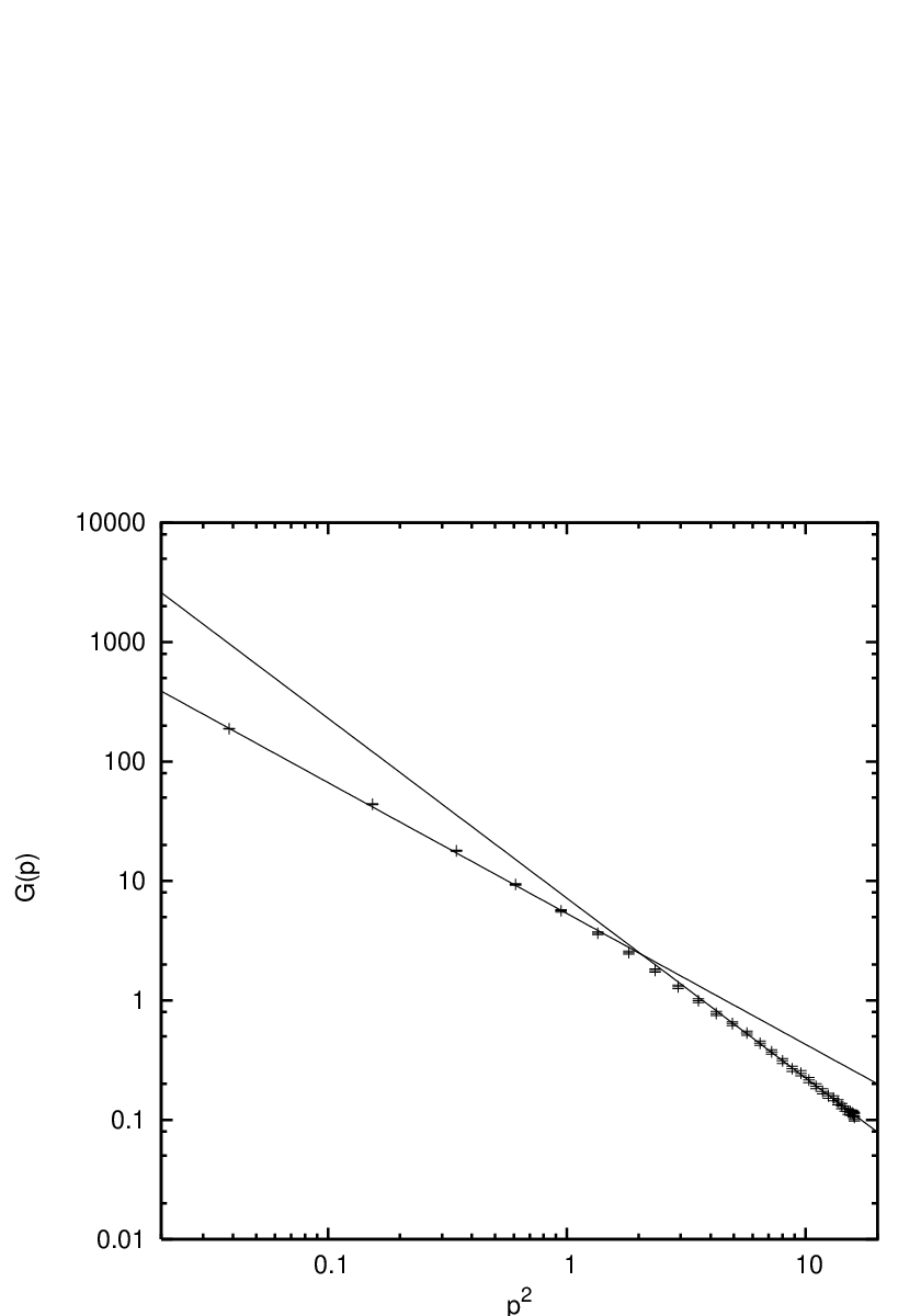
In the gluon case we find that data at small momenta are best fitted with . Then, the exponent is very close to 0.5 in the 3d case (see Table 1) if one uses for the fit the range with . A slightly larger or smaller value for is obtained if one uses respectively or . For momenta larger than the best fit is obtained considering . In this case (see Table 2) the exponent is very close to 0.35 and this value is essentially independent of the value of . In both cases the effects due to the breaking of rotational invariance are relatively small, as expected (see discussion in Section II.2 above). Finally, we tried a fit of all the data with (see Table 3). Clearly, in this case one finds for a kind of average between the value 0.5 found at small momenta and the value 0.35 obtained at large momenta. It is interesting to notice that a value very close to the conformal solution is obtained for the largest lattice volumes and for momenta of the type and . As an example we report in Fig. 2 the fits obtained at small and at large momenta for the lattice volume and for data corresponding to the momenta .
One can also check that the gluon propagator violates reflection positivity. Actually, for all cases we find that is already negative. [Of course, is always positive.] In Fig. 3 we show as a function of the space-time separation for the lattice volume when considering momenta of the type . Following Ref. [49], we fitted the data using a sum of two Stingl-like [89] propagators with . We found a good description of the data (see again Fig. 3) by fixing and with and . Also, by comparing these data to results obtained in the scaling region [49], one can use the value of where starts to oscillate around zero as an input for fixing the lattice spacing. From Fig. 3 this happens at , giving (see Figure 5 in Ref. [49]). This is in quantitative agreement with the values obtained in [73] (see Section I.5 above).

We also consider the volume dependence of and the bounds introduced in [47]. As one can see from Fig. 4, these bounds are well satisfied. Compared to the results obtained at finite (nonzero) (see Fig. 1 in [47]), we find that the values of are closer to the upper bound than to the lower one. We have also checked that we can extrapolate the data for and for the upper and the lower bounds to a finite nonzero value as well as to zero (see Table 4). However, considering the value of , our data seem to prefer an extrapolation to (see also Fig. 4).
Let us note that the above result is in agreement with what observed in Ref. [90], i.e. in the 3d case volumes up to are not large enough in order to have a complete control over the extrapolation to at . This suggests that — for the zero-momentum propagator — simulations for and for values in the scaling region are essentially equivalent. In other words, the value of seems to be related only to the thermodynamic limit () and is not affected by the value of the lattice spacing. This peculiar behavior at may be related to the fact that the gauge-fixing condition does not play a role in this case. Also, one might argue that is simply a measure of the zero modes of the gluon field, whose value is of course strongly affected by the lattice size. The situation is different for . Indeed, while at the propagator is decreasing with for all lattice volumes and momenta, for values of in the scaling region one sees a decreasing propagator only for large enough lattice volume and for momenta below a certain value . Also, at finite-size effects for are very small or null (see Fig. 5 below and compare to Fig. 1 in Ref. [1]), while for one sees large finite-size effects for .
| fit | ||||
|---|---|---|---|---|
| lower bound | 0.048(3) | 0.5(4) | 1.2(4) | 4.22 |
| 0.30(2) | 3(2) | 1.2(3) | 3.42 | |
| upper bound | 0.46(3) | 4(3) | 1.2(3) | 3.62 |
| fit | ||||
| lower bound | 0.12(2) | 0.20(4) | 13.0 | |
| 0.74(9) | 0.20(4) | 13.5 | ||
| upper bound | 1.1(1) | 0.20(4) | 12.3 |

II.3.2 4d gluon propagator
We did the same fitting analysis also in the 4d case for the gluon propagator at the lattice volume . As shown in Tables 5, 6 and 7 we find and at small momenta (using the fit with ), while the fit for (with ) gives and . (The fits corresponding to the range of small and large momenta are shown together with the data in Figs. 6 and 7.) These results essentially do not change by cutting the data in Tables 5 and 6 at or at . However, contrary to the 3d case, our data for can also be described by the fitting function with . Indeed, in this case, a good fit — with and — is obtained with and . Finally, a fit using all the momenta and suggests a kind of average value for , i.e. . Thus, the fits suggest a value for close to the scaling solution result only if one ignores the data at small momenta and forces the parameter to be zero.
As in the 3d case, the effects due to violation of rotational symmetry are clearly small. Also, violation of reflection positivity is observed already at and the gluon propagator in position space is well described by a sum of two Stingl-like propagators with (see Fig. 8). Note that the values of the masses are not very different from the 3d case. Finally, as explained in Section II.3.1 above, one can fix the lattice spacing by comparing these data to results obtained in the scaling region. In particular, considering our data at for , we find that for . Then, from Fig. 8, we find as in the 3d case.
| momenta | |||||
|---|---|---|---|---|---|
| 1 | 0.446(4) | 0.095(5) | 0.85(3) | 11 | 1.33 |
| 2 | 0.460(5) | 0.095(6) | 0.83(4) | 6 | 0.85 |
| 3 | 0.41(4) | 0.14(4) | 0.67(8) | 4 | 1.28 |
| 4 | 0.45(2) | 0.08(2) | 0.9(2) | 3 | 1.97 |
| momenta | ||||
|---|---|---|---|---|
| 1 | 0.533(3) | 0.570(3) | 17 | 0.76 |
| 2 | 0.558(4) | 0.562(2) | 21 | 0.86 |
| 3 | 0.561(6) | 0.561(3) | 23 | 0.99 |
| 4 | 0.531(6) | 0.566(2) | 24 | 0.97 |
| momenta | |||||
|---|---|---|---|---|---|
| 1 | 0.436(4) | 0.103(5) | 0.76(1) | 30 | 1.60 |
| 2 | 0.430(9) | 0.13(1) | 0.70(1) | 29 | 2.20 |
| 3 | 0.39(2) | 0.17(2) | 0.65(1) | 29 | 1.38 |
| 4 | 0.41(1) | 0.13(2) | 0.68(1) | 29 | 1.19 |


II.3.3 3d ghost propagator
We now consider the data obtained for the ghost propagator in the 3d case. [Note that in this case we did not evaluate the propagator for the lattice volume .] As said above, we tried a fit using the function . Results are reported in Table 8. One clearly sees that the infrared exponent decreases as the lattice volume increases, in agreement with [57, 38]. In this case the effects due to the violation of rotational symmetry are more evident. Indeed, the exponent is systematically smaller for momenta along the axes. This is probably due to the fact that along the axes one can consider smaller momenta, for which the ghost propagator is less enhanced.
By looking at Fig. 9 it is clear that this fit, with only one term, can be improved. In particular, considering the results reported in [2, 1, 3], one can try to see how the exponent depends on the value of . To this end we have ordered the data points by the value of and divided them in sets of ten data points. Then, we did a separate fit in each interval, again using the fitting function . Results for the lattice volume are reported in Table 9. One clearly sees that the exponent increases with (see also Fig. 10) and it is usually larger for the type of momenta . The same is observed for the other lattice volumes. This result is actually well-known. Indeed, all lattice studies of the ghost propagator [57, 91, 92] have found that is enhanced compared to the tree-level propagator at intermediate momenta. (We will comment again on this in the Conclusions.)
| momenta | ||||||
|---|---|---|---|---|---|---|
| 1 | 0.382 | 3.94(3) | 0.260(8) | 3 | 0.39 | |
| 2 | 0.764 | 3.9(1) | 0.35(2) | 3 | 1.75 | |
| 1 | 0.098 | 3.77(5) | 0.209(7) | 8 | 4.15 | |
| 2 | 0.196 | 3.57(6) | 0.28(1) | 8 | 3.06 | |
| 1 | 0.0246 | 3.64(8) | 0.171(7) | 18 | 14.2 | |
| 2 | 0.0492 | 3.38(7) | 0.220(8) | 18 | 5.59 | |
| 1 | 0.0110 | 3.74(8) | 0.144(5) | 28 | 29.2 | |
| 2 | 0.0219 | 3.89(8) | 0.192(8) | 28 | 16.7 | |
| 1 | 0.0062 | 3.84(9) | 0.127(6) | 38 | 18.4 | |
| 2 | 0.0123 | 3.50(7) | 0.164(6) | 38 | 7.02 | |
| 1 | 0.0039 | 4.1(1) | 0.110(5) | 48 | 19.4 | |
| 2 | 0.0079 | 3.46(8) | 0.154(5) | 48 | 9.91 |

| momenta | |||||
|---|---|---|---|---|---|
| 0.0039 | 0.38 | 1 | 5.0(2) | 0.070(6) | 11.2 |
| 0.0079 | 0.76 | 2 | 4.4(1) | 0.102(7) | 4.40 |
| 0.46 | 1.38 | 1 | 4.00(2) | 0.21(1) | 0.17 |
| 0.92 | 2.76 | 2 | 3.98(5) | 0.29(2) | 0.19 |
| 1.50 | 2.62 | 1 | 3.7(1) | 0.08(5) | 0.19 |
| 3.01 | 5.24 | 2 | 4.2(1) | 0.33(3) | 0.04 |
| 2.74 | 3.62 | 1 | 6(1) | 0.6(1) | 0.31 |
| 5.47 | 7.24 | 2 | 3(1) | 0.3(1) | 0.28 |
II.3.4 4d ghost propagator
| momenta | ||||
|---|---|---|---|---|
| 1 | 0.0096 | 5.4(2) | 0.075(7) | 250 |
| 2 | 0.0193 | 4.6(2) | 0.128(9) | 238 |
| 3 | 0.0289 | 4.2(1) | 0.16(1) | 127 |
| 4 | 0.0385 | 4.0(1) | 0.19(1) | 55.3 |
| momenta | |||||
|---|---|---|---|---|---|
| 0.0096 | 0.59 | 1 | 6.4(2) | 0.036(7) | 101 |
| 0.0193 | 1.17 | 2 | 5.8(2) | 0.06(1) | 114 |
| 0.0289 | 1.76 | 3 | 5.4(2) | 0.09(1) | 65.4 |
| 0.0385 | 2.34 | 4 | 5.3(2) | 0.10(1) | 18.6 |
| 0.73 | 2 | 1 | 5.192(9) | 0.223(5) | 0.13 |
| 1.46 | 4 | 2 | 5.28(3) | 0.300(6) | 0.11 |
| 2.19 | 6 | 3 | 5.64(5) | 0.389(7) | 0.09 |
| 2.92 | 8 | 4 | 5.8(2) | 0.39(2) | 0.18 |
| 2.20 | 3.41 | 1 | 5.78(8) | 0.38(1) | 0.06 |
| 4.39 | 6.83 | 2 | 5.94(9) | 0.403(9) | 0.03 |
| 6.59 | 10.2 | 3 | 5.8(2) | 0.39(1) | 0.04 |
| 8.78 | 13.7 | 4 | 7.2(7) | 0.51(4) | 0.10 |
| 3.55 | 4 | 1 | 5.8(2) | 0.39(2) | 0.01 |
| 7.09 | 8 | 2 | 5.8(4) | 0.39(3) | 0.02 |
| 10.6 | 12 | 3 | 19(6) | 0.9(1) | 0.24 |
| 14.2 | 16 | 4 | 7(2) | 0.5(1) | 0.08 |
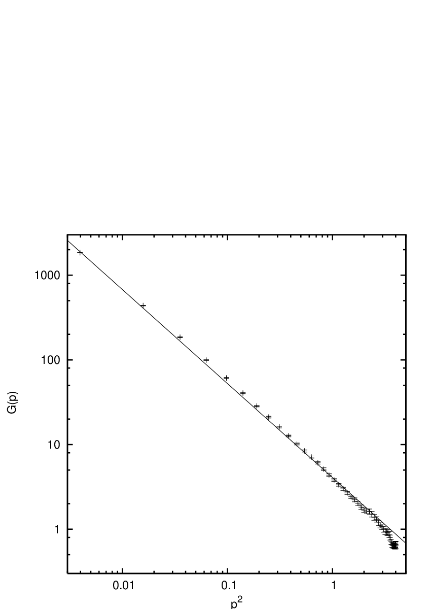
Finally, data for the ghost propagator in the 4d case show again (see Table 10) that the exponent depends on the type of momenta and systematically increases when one considers momenta closer to the diagonal than to the axes. Also, the exponent increases with (see Table 11 and Fig. 11), going from a very small value — close to zero — at small up to almost 1 for the largest momenta and for momenta along the diagonal. This can be seen also in Fig. 12, where an effective exponent has been evaluated using the relation , where and are the values of the ghost propagator at two nearby momenta and . The plot is done as a function of the average momentum . The errors have been evaluated using the so-called bootstrap method with 2000 samples. For clarity, we show only results with a relative error smaller than 50% and with a positive value for (this criterion selects about 70% of the data). One clearly sees that the effective exponent is monotonically increasing. The situation is very different in the gluon sector, where indeed a scaling solution can be used to fit the data. As one can see in Fig. 13, the effective exponent is essentially constant in this case. Moreover, at small momenta one finds , in agreement with the massive solution, and at large momenta the effective exponent is still very close to this value. Note that a constant shift of 0.5 is built into the definition of the gluon exponent . Thus, numerical results in the gluon sector should be rather quoted as , in order to convey a clear indication of the precision of the results.


II.3.5 A massive fit for the ghost propagator
The analysis above has shown that the scaling solution does not describe the ghost sector. Indeed, one cannot find a reasonably large range of momenta where the data can be fitted by a power-law with a given value of the IR exponent .
On the other hand, the ghost-propagator data are well described by the fitting function , recently proposed in [24], which gives a free ghost propagator in the infrared limit. The parameter can be interpreted as a gluon mass [24]. Also note that this function corresponds to the small-momentum limit of the fitting function used in Ref. [42] to fit the ghost data in 3d and in 4d for values of in the scaling region. Using the fitting function above we obtain, in the 3d case, the parameters , and with using the data (see Fig. 14). Using all the data one finds , and with . A similar fit in the 4d case gives , and with using the data (see Fig. 15). Using all the data one finds , and with (see Fig. 16).


For a comparison with Ref. [1] — see Eq. (19c) and Fig. 9 of that reference — we have also tried a global fit using for the ghost dressing function the Ansatz . The resulting fit gives with in 3d and with in the 4d case (see Fig. 17). Thus, the value of is clearly worse when compared to the logarithmic behavior considered above. In particular, from Fig. 17 one can see that the power-law behavior cannot describe well the “curvature” of the data, underestimating the data at small and at large momenta and overshooting the numerical results at intermediate momenta. This is of course not a surprise since we have clearly shown in the previous subsection that a single power-law does not describe the ghost data, unless one selects a very small interval of momenta. In the 4d case, this result does not improve if one forces the exponent to be equal to 0.562, as done in Fig. 9 of [1]. Indeed, in this case we find and with (see Fig. 18).
One should also observe that the function considered above and in Ref. [1] is not a truly scaling solution . Indeed, while the latter is characterized by a constant value for the exponent , for one has an effective exponent . This effective exponent is monotonically increasing with , becoming constant and equal to only for very large momenta. Thus, is trying to describe the lattice data, characterized by an exponent increasing with the momentum, while “suggesting” a possible scaling behavior, i.e. a function with a constant exponent. In fact, as we have shown above, the data are much better described by the massive solution , suggested by a recent analytic study [24]. On the other hand, a function such as is very poorly justified from the theoretical point of view. In particular, such a fitting function for the ghost dressing function implies a fit for the ghost propagator. We do not see any theoretical reason that the mass scale should affect only “part” of the power-law behavior of the propagator. Here we have also tried a fit to the ghost-propagator data using : the result is very poor, with [and ].
Finally, that a simple power-law is not capable of describing the lattice data should also be clear looking at Fig. 5 of Ref. [1], where it is evident that the exponent depends on the momentum considered, and from Fig. 9 of the same reference, where one sees that the fit systematically underestimates the data at intermediate momenta. Actually, at the end of Sec. III of Ref. [1] the authors clearly say that a true scaling solution, i.e. their Eq. (19a), gives a very poor description of the ghost data and that their preferred fitting function is , which only reminds one of a possible scaling behavior. This is probably the reason that induced the authors of [1] to conclude in favor of a scaling solution at large momenta in the ghost sector. As already stressed above, we do not agree with this conclusion.


III Conclusions
We have studied numerically the infrared behavior of Landau-gauge gluon and ghost propagators at lattice parameter , considering 3d lattices of volumes up to and 4d lattices of volume . By carrying out a careful fit analysis of the proposed behavior according to the scaling or to the massive solutions of DSE, we find that our data strongly support the massive solution, i.e. a finite gluon propagator and an essentially free ghost propagator in the infrared limit . Moreover, the gluon propagator as a function of the space-time separation violates reflection positivity and it is well-described by a sum of two Stingl-like propagators. These results are in qualitative agreement with data obtained at finite in the scaling region.
We should stress that, in agreement with Refs. [2, 1, 3], a scaling solution appears in the gluon sector if one neglects the data at small momenta. As explain in Section I.5 above, we do not see any reason for excluding those data from the analysis. In particular, discretization effects at small momenta are under control and the large effects observed in Ref. [1] are probably only due to the bad scaling properties of the modified Landau gauge. Moreover, the value of clearly depends on the way the fits are done. In particular, a value close to the preferred value of the scaling solution, i.e. in dimensions, is obtained only with very specific and ad-hoc fits. In any case, we believe that the scaling solution is clearly excluded by the ghost sector and we definetively do not agree on this point with the analysis and the conclusions presented in [2, 1, 3]. Indeed, in this case, the IR exponent depends on the interval considered, increasing essentially monotonically as the momentum increases, i.e. it is impossible to find a decent “window” giving a constant value for . On the other hand, we have shown that the data for the ghost propagator are very well described by a simple function, recently suggested by an analytic study presented in [24]. This function clearly supports the so-called massive solution.
As for the ongoing discussion about massive solution versus conformal scaling, we remark that the lattice results may be summarized as follows.
- •
- •
- •
- •
In the so-called gauges, which interpolate between the Landau gauge () and the Coulomb gauge (), one clearly sees [96] that the behavior of the transverse gluon propagator gets modified when goes from 1 to 0, becoming closer and closer to the behavior obtained in Coulomb gauge as becomes smaller and smaller.
The simulations cited above are essentially all done in the same way, i.e. in most of the cases by ignoring effects due to Gribov copies, by using a standard discretization for the lattice action, for the gluon field and for the gauge-fixing condition and by using one of the standard gauge-fixing algorithms. Recently, to rescue the conformal solution in Landau gauge, several authors have explained the lattice Landau data by evoking supposedly (very) large effects due to Gribov copies, discretization effects and bias related to the use of the usual gauge-fixing algorithms. Of course, one has to verify that all possible sources of systematic effects are indeed under control in a numerical simulation. On the other hand, it seems unlikely to us that these effects would show up in some cases of the simulations described above and not in others. For example, why would the 2d Landau-gauge case be conformal and not the 3d and 4d cases if the same code is used in these three cases? Why should Gribov-copy effects be so important in 3d and 4d Landau gauge and not in 2d Landau gauge and, even more strikingly, in 4d Coulomb gauge, where one would expect stronger effects since the transversality condition is imposed separately on each time slice? In our view, present lattice data are simply telling us that the infrared behavior of gluon and ghost propagators in Landau, Coulomb and gauge depends on the gauge-fixing condition and on the dimensionality of the system (as, for example, the critical behavior of statistical mechanical systems). We believe that the present challenge is to understand why this is the case and that the bounds introduced by us in Ref. [47] and their interpretation in terms of magnetization and susceptibility of the gluon field could be a key ingredient in a simple explanation of present lattice results in Landau gauge.
Finally a remark about color confinement. As said in the Conclusion of Ref. [42], we point out that the behavior of gluon and ghost propagators at very small momenta is probably not so important for the explanation of confinement. Indeed, why should the behavior of a Green function at a few , i.e. for a space separation of about , be relevant for hadron physics, since the typical hadronic scale is of order of ? Let us recall that in a recent paper [97] it has been shown that the appearance of a linearly-rising potential is related (in Landau and in Coulomb gauge) to the momentum-space gluon configuration for . In this region one can indeed observe strong non-perturbative effects in the gluon and in the ghost propagators in Landau gauge: the gluon propagator violates reflection positivity and the ghost propagator is enhanced when compared to the tree-level behavior. Thus, some important predictions of the Gribov-Zwanziger scenario are still verified and, at the same time, one can try to relate the massive solution to the requirement of color confinement as in Refs. [30, 31, 32].
IV Acknowledgements
We thank the organizers of the workshop on Non perturbative Aspects of Field Theories (Morelia ’09), where this work was presented, for providing a very stimulating atmosphere for discussions, in such a beautiful setting.
We acknowledge partial support from the Brazilian Funding Agencies FAPESP and CNPq. The work of T.M. is supported also by a fellowship from the Alexander von Humboldt Foundation. Most of the simulations reported here have been done on the IBM supercomputer at São Paulo University (FAPESP grant # 04/08928-3).
References
- [1] A. Sternbeck and L. von Smekal, arXiv:0811.4300 [hep-lat].
- [2] A. Sternbeck and L. von Smekal, PoS LATTICE2008, 267 (2008).
- [3] A. Sternbeck and L. von Smekal, arXiv:0812.3268 [hep-lat].
- [4] V.N. Gribov, Nucl. Phys. B 139, 1 (1978).
- [5] D. Zwanziger, Nucl. Phys. B 412, 657 (1994).
- [6] D. Zwanziger, arXiv:0904.2380 [hep-th].
- [7] For a short review of the Gribov-Zwanziger approach see A. Cucchieri and T. Mendes, arXiv:0809.2777 [hep-lat].
- [8] T. Kugo and I. Ojima, Prog. Theor. Phys. Suppl. 66, 1 (1979) [Erratum-ibid. 71, 1121 (1984)].
- [9] T. Kugo, arXiv:hep-th/9511033.
- [10] R. Alkofer and L. von Smekal, Phys. Rept. 353, 281 (2001).
- [11] D. Zwanziger, Phys. Rev. D 67, 105001 (2003).
- [12] D. Zwanziger, Phys. Lett. B 257, 168 (1991).
- [13] G. Dell’Antonio and D. Zwanziger, Nucl. Phys. B 326, 333 (1989).
- [14] D. Dudal, S.P. Sorella, N. Vandersickel and H. Verschelde, arXiv:0904.0641 [hep-th].
- [15] See for example C.D. Roberts and A.G. Williams, Prog. Part. Nucl. Phys. 33, 477 (1994).
- [16] R. Alkofer, M.Q. Huber and K. Schwenzer, arXiv:0801. 2762 [hep-th].
- [17] C.S. Fischer and J.M. Pawlowski, Phys. Rev. D 75, 025012 (2007).
- [18] L. von Smekal, A. Hauck and R. Alkofer, Annals Phys. 267, 1 (1998) [Erratum-ibid. 269, 182 (1998)].
- [19] D. Zwanziger, Phys. Rev. D 65, 094039 (2002).
- [20] J.M. Pawlowski et al., Phys. Rev. Lett. 93, 152002 (2004).
- [21] A.C. Aguilar and A.A. Natale, JHEP 0408, 057 (2004).
- [22] Ph. Boucaud et al., JHEP 0606, 001 (2006).
- [23] C.S. Fischer, J. Phys. G 32, R253 (2006).
- [24] A.C. Aguilar, D. Binosi and J. Papavassiliou, Phys. Rev. D 78, 025010 (2008).
- [25] M.Q. Huber et al., Phys. Lett. B 659, 434 (2008).
- [26] Ph. Boucaud et al. JHEP 0806, 012 (2008).
- [27] Ph. Boucaud et al., JHEP 0806, 099 (2008).
- [28] C.S. Fischer, A. Maas and J.M. Pawlowski, arXiv:0810. 1987 [hep-ph].
- [29] R. Alkofer and J. Greensite, J. Phys. G 34, S3 (2007).
- [30] M. Chaichian and K. Nishijima, Eur. Phys. J. C 47, 737 (2006).
- [31] J.M. Cornwall, Nucl. Phys. B 157, 392 (1979).
- [32] J. Braun, H. Gies and J.M. Pawlowski, PoS CONFINEMENT8, 044 (2008).
- [33] D. Dudal et al., Phys. Rev. D 77, 071501 (2008).
- [34] D. Dudal et al., Phys. Rev. D 78, 065047 (2008).
- [35] D. Dudal et al., Phys. Rev. D 78, 125012 (2008).
- [36] D. Dudal et al., arXiv:0808.3379 [hep-th].
- [37] M. Frasca, Phys. Lett. B 670, 73 (2008).
- [38] A. Cucchieri and T. Mendes, PoS (LATTICE 2007) 297.
- [39] I.L. Bogolubsky et al., PoS LAT2007, 290 (2007).
- [40] A. Sternbeck et al., PoS LAT2007, 340 (2007).
- [41] O. Oliveira and P.J. Silva, arXiv:0705.0964 [hep-lat].
- [42] A. Cucchieri and T. Mendes, Phys. Rev. D 78, 094503 (2008).
- [43] V.G. Bornyakov, V.K. Mitrjushkin and M. Muller-Preussker, arXiv:0812.2761 [hep-lat].
- [44] I.L. Bogolubsky, E.M. Ilgenfritz, M. Muller-Preussker and A. Sternbeck, Phys. Lett. B 676, 69 (2009).
- [45] M. Gong et al., arXiv:0811.4635 [hep-lat].
- [46] A. Maas, Phys. Rev. D 75, 116004 (2007).
- [47] A. Cucchieri and T. Mendes, Phys. Rev. Lett. 100, 241601 (2008).
- [48] K. Langfeld, H. Reinhardt and J. Gattnar, Nucl. Phys. B 621, 131 (2002).
- [49] A. Cucchieri, T. Mendes and A.R. Taurines, Phys. Rev. D 71, 051902 (2005).
- [50] O. Oliveira and P.J. Silva, Braz. J. Phys. 37, 201 (2007).
- [51] P.O. Bowman et al., Phys. Rev. D 76, 094505 (2007).
- [52] A. Cucchieri, Nucl. Phys. B 521, 365 (1998).
- [53] A. Sternbeck, E.M. Ilgenfritz and M. Muller-Preussker, Phys. Rev. D 73, 014502 (2006).
- [54] A. Cucchieri, A. Maas and T. Mendes, Phys. Rev. D 74, 014503 (2006).
- [55] A. Cucchieri and T. Mendes, arXiv:0812.3261 [hep-lat].
- [56] A. Cucchieri, AIP Conf. Proc. 892, 22 (2007).
- [57] A. Cucchieri, Nucl. Phys. B 508, 353 (1997).
- [58] P.J. Silva and O. Oliveira, Nucl. Phys. B 690, 177 (2004).
- [59] P.J. Silva and O. Oliveira, PoS LAT2007, 333 (2007).
- [60] A. Maas, arXiv:0808.3047 [hep-lat]. Phys. Rev. D 79, 014505 (2009).
- [61] D.B. Leinweber et al., Phys. Rev. D 60, 094507 (1999) [Erratum-ibid. D 61, 079901 (2000)].
- [62] J.P. Ma, Mod. Phys. Lett. A 15, 229 (2000).
- [63] F. de Soto and C. Roiesnel, JHEP 0709, 007 (2007).
- [64] E. Shintani et al., arXiv:0807.0556 [hep-lat].
- [65] F. Di Renzo, Nucl. Phys. Proc. Suppl. 53 (1997) 819.
- [66] L. Giusti et al., Phys. Lett. B 432, 196 (1998).
- [67] S. Furui and H. Nakajima, Nucl. Phys. Proc. Suppl. 73, 865 (1999).
- [68] F.D.R. Bonnet et al., Austral. J. Phys. 52, 939 (1999).
- [69] A. Cucchieri and F. Karsch, Nucl. Phys. Proc. Suppl. 83, 357 (2000).
- [70] L. von Smekal et al., PoS LAT2007, 382 (2007).
- [71] J.C.R. Bloch et al., Nucl. Phys. B 687, 76 (2004).
- [72] A. Cucchieri, Phys. Lett. B 422, 233 (1998).
- [73] P. de Forcrand and M. Fromm, arXiv:0907.1915 [hep-lat].
- [74] P. de Forcrand and S. Kim, Phys. Lett. B 645, 339 (2007).
- [75] A. Cucchieri and T. Mendes, in preparation.
- [76] See for example the introduction to strong-coupling expansion in Introduction to Quantum Fields on a Lattice, Jan Smit (Cambridge University Press, 2002, Cambridge UK).
- [77] A. Cucchieri, poster presented at the workshop Infrared QCD in Rio, held in Rio de Janeiro in June 2006 (http://www.dft.if.uerj.br/irqcd06/).
- [78] A. Cucchieri et al., Phys. Rev. D 76, 114507 (2007).
- [79] A. Cucchieri et al., PoS LAT2007, 322 (2007).
- [80] A. Maas and S. Olejnik, JHEP 0802, 070 (2008).
- [81] A. Cucchieri, T. Mendes, O. Oliveira and P.J. Silva, Int. J. Mod. Phys. E 16, 2931 (2007).
- [82] A. Cucchieri and T. Mendes, Nucl. Phys. B 471, 263 (1996).
- [83] Ph. Boucaud et al., Phys. Rev. D 72, 114503 (2005).
- [84] M. Creutz, Phys. Rev. D 21, 2308 (1980).
- [85] See the Introduction of A. Cucchieri and T. Mendes, Comput. Phys. Commun. 154, 1 (2003).
- [86] A. Cucchieri and T. Mendes, Nucl. Phys. Proc. Suppl. 53, 811 (1997).
- [87] T. Mendes et al., arXiv:0809.3741 [hep-lat].
- [88] See for example D. Becirevic et al., Phys. Rev. D 60, 094509 (1999).
- [89] M. Stingl, Phys. Rev. D 34, 3863 (1986) [Erratum-ibid. D 36, 651 (1987)].
- [90] A. Cucchieri, T. Mendes and A.R. Taurines, Phys. Rev. D 67, 091502 (2003).
- [91] S. Furui and H. Nakajima, Phys. Rev. D 69, 074505 (2004).
- [92] J. Gattnar, K. Langfeld and H. Reinhardt, Phys. Rev. Lett. 93, 061601 (2004).
- [93] A. Cucchieri and D. Zwanziger, Phys. Rev. D 65, 014001 (2002).
- [94] A. Cucchieri and D. Zwanziger, Phys. Lett. B 524, 123 (2002).
- [95] G. Burgio, M. Quandt and H. Reinhardt, Phys. Rev. Lett. 102, 032002 (2009).
- [96] A. Cucchieri, A. Maas and T. Mendes, Mod. Phys. Lett. A 22, 2429 (2007).
- [97] A. Yamamoto and H. Suganuma, Phys. Rev. Lett. 101, 241601 (2008).