A Compound Josephson Junction Coupler for Flux Qubits With Minimal Crosstalk

The choice of architecture of a prototype solid state quantum information processor is primarily driven by the algorithm that the designer wishes to implement. Within the field of superconducting quantum devices, at least two distinct architectures have arisen. Gate model algorithms require qubits with long-lived excited states and dynamic couplings. Recent efforts have focused upon charge-like [1] and phase [2] qubits coupled to microwave resonators. Adiabatic quantum algorithms [3, 4] require qubits whose groundstate encode binary variables and static couplings. One implementation involves a network of inductively coupled flux qubits [5]. The Hamiltonian for this architecture is that of a quantum Ising spin glass,

The authors of Ref. [8] proposed the use of an rf-SQUID to implement tunable $M_{ij}$. Experiments on systems of coupled flux qubits verified that such couplers did perform as anticipated [9]. However, additional work not reported in the literature revealed two serious deficiencies: First, the tuning mechanism involves threading flux through the rf-SQUID loop, thus inducing a large persistent current $I_{p}$ that, in turn, biases the qubits. This is a significant problem if the qubit biases need to be controlled to high precision atop what can be a very large nonlinear crosstalk imparted by the coupler. Second, $M_{ij}=0$ can only be achieved if $\beta\equiv 2\pi LI_{c}/\Phi_{0}<1$, where $L$ and $I_{c}$ are the rf-SQUID inductance and critical current, respectively. On the other hand, in order to achieve appreciable non-zero coupling it proved necessary to design devices with $\beta\gtrsim 0.9$. Such devices were acutely sensitive to fabrication variations, where higher than expected $I_{c}$ could make $M_{ij}=0$ unattainable. Thus the rf-SQUID coupler proved troublesome in practice. Note that the dc-SQUID [8, 10] and the unipolar [11] couplers suffer from similar deficiencies. The challenge was then to design a tunable $M_{ij}$ that invokes minimal $I_{p}$ and is robust against fabrication variations.

Our efforts to identify a satisfactory coupler design led us to consider the compound Josephson junction (CJJ) rf-SQUID, as depicted in Fig. 1. The CJJ rf-SQUID comprises a superconducting loop of inductance $L$ that is interrupted by a smaller loop of inductance $L_{\text{co}}$ containing two Josephson junctions with critical currents $I_{c1}$ and $I_{c2}$. Devices with this general topology can take on a number of guises: The CJJ rf-SQUID can be used as a qubit when designed with relatively low $I_{c}=I_{c1}+I_{c2}\lesssim 3\,\mu$A, $L$ chosen such that $\beta\lesssim 2$, low net capacitance across the junctions $C$ and biased such that its potential energy is bistable [12, 13]. The CJJ rf-SQUID can also be used as a latching readout when designed with a substantial $I_{c}\gtrsim 10\,\mu$A, $L$ chosen such that $\beta\gtrsim 1.2$, large $C$ and having its potential swept from being monostable to bistable [14]. We focus herein upon a CJJ rf-SQUID designed with a modest $I_{c}$, $L$ chosen such that $\beta\lesssim 1.2$ and operated with a monostable potential. In Fig. 1 the closed loops are subjected to external flux biases $\Phi_{\text{act}}^{x}\equiv\Phi_{0}\varphi_{\text{act}}^{x}/2\pi$ and $\Phi_{\text{co}}^{x}\equiv\Phi_{0}\varphi_{\text{co}}^{x}/2\pi$. The symbols have been chosen to indicate that $\Phi_{\text{act}}^{x}$ is an actuator for perturbing the device and $\Phi_{\text{co}}^{x}$ represents the control signal. Let the phase across the junctions be $\varphi_{1}$ and $\varphi_{2}$. The Hamiltonian for this device can be written as

Let the device described by Eq. (3) be connected to two qubits via mutual inductances $M_{\text{co},1}$ and $M_{\text{co},2}$. The mutual inductance between the qubits will be

While rf-SQUID and CJJ rf-SQUID couplers possess similar expressions for $\chi^{(1)}$, the latter holds two advantages: First, the CJJ coupler can be operated with $\Phi_{\text{act}}^{x}=0$ and tuned via $\Phi_{\text{co}}^{x}$. If $I_{c-}/I_{c+}\ll 1$, then $\varphi_{\text{act}}^{0}\ll 1$ and Eq. (6) yields $\varphi_{\text{act}}\approx 0$. Equation (5) then predicts that $I_{\text{act}}^{p}\approx 0$. Thus the CJJ coupler need not invoke large persistent currents (on the order of $I_{c+}$) when being tuned. Second, the CJJ coupler is usable over the range of $\Phi_{\text{co}}^{x}$ for which $-\text{min}\left[1,\beta_{\text{eff}}(0)\right]\lesssim\beta_{\text{eff}}(\varphi_{\text{co}}^{x})\leq\beta_{\text{eff}}(0)$ when $\Phi_{\text{act}}^{x}=0$, where the lower bound has been imposed by the condition that $V(\varphi_{\text{act}})$ be monostable. Thus the utility of the CJJ coupler is not compromised if $\beta_{\text{eff}}(0)>1$. As such, this device is robust against fabrication variations.

To test the CJJ rf-SQUID coupler, we fabricated a circuit containing 8 CJJ rf-SQUID flux qubits [12, 13], each inductively coupled to its own hysteric dc-SQUID readout [15], and connected by a network of 16 CJJ rf-SQUID couplers. The chip was fabricated from an oxidized Si wafer with Nb/Al/Al₂O₃/Nb trilayer junctions, four Nb wiring layers capped with SiN and separated by planarized PECVD SiO₂. The chip was mounted to the mixing chamber of a dilution refrigerator regulated at $T=40\,$mK inside a Sn superconducting magnetic shield with a residual field in the vicinity of the chip $\lesssim 1\,$nT. External current biases were provided by room temperature current DACs whose outputs were low pass filtered with $f_{c}\approx 5\,$MHz using a combination of lumped element and copper powder filters secured to the mixing chamber.

A schematic of a coupler and a pair of qubits is depicted in Fig. 2. The coupler is controlled via bias currents that are coupled to the device through mutual inductances $M_{\text{co}}$ and $M_{\text{act}}$, respectively. These give rise to the fluxes $\Phi_{\text{co}}^{x}$ and $\Phi_{\text{act}}^{x}$. The qubits are controlled via fluxes $\Phi_{\text{cjj}\alpha}^{x}$ and $\Phi_{q\alpha}^{x}$ ($\alpha=1,2$) as described in Ref. [13]. The qubits interact with the coupler via mutual inductances $M_{\text{co},\alpha}$. For brevity, we present results from a single coupler in this paper and note that $M_{\text{eff}}(\Phi_{\text{co}}^{x})$ was identical to $\lesssim 5\%$ for all 16 couplers on this chip. For the particular coupler described herein, the relevant qubit critical currents were $I_{q\alpha}^{c}=3.25\pm 0.01\,\mu$A and qubit inductances were $L_{q1(2)}=290(308)\pm 5\,$pH when $\Phi_{\text{co}}^{x}=0$.

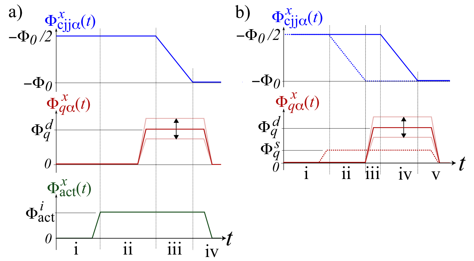
The flux waveforms used to obtain $M_{\text{act}}$ are depicted in Fig. 3a. In this case, $\Phi_{\text{co}}^{x}$ was held constant while the detector qubit ($\alpha=d$) was annealed in the presence of a pulse on $\Phi_{\text{act}}^{x}(t)$ of amplitude $\Phi_{\text{act}}^{i}$ and a pulse on $\Phi_{q\alpha}^{x}(t)$ of amplitude $\Phi_{q}^{d}$. The sequence involves initializing the qubit in a monostable potential with no net flux biases (i), setting $\Phi_{\text{act}}^{x}$ and $\Phi_{q\alpha}^{x}$ (ii), raising the detector qubit’s tunnel barrier to maximum height (iii) and then returning $\Phi_{\text{act}}^{x}$ and $\Phi_{q\alpha}^{x}$ to zero prior to reading the state of the detector qubit (iv). The result of this process is that the state of the detector qubit becomes trapped in one of its two counter-circulating persistent current states, denoted as $\left|{0}\right\rangle$ and $\left|{1}\right\rangle$. Repeating this sequence to gather statistics then yielded the probability of finding the detector in $\left|{0}\right\rangle$, $P_{0}$. Using software feedback, we adjusted $\Phi_{q}^{d}$ to track the displacement of the detector’s degeneracy point $\Phi_{q\alpha}^{0}$, defined as the bias for which $P_{0}=1/2$, to within $\pm 0.02\,$m$\Phi_{0}$. We have defined $\Phi_{q\alpha}^{0}\equiv 0$ with respect to the degeneracy point obtained with $\Phi_{\text{co}}^{x}=0$ and $\Phi_{\text{act}}^{x}=0$. Mapping $\Phi_{q\alpha}^{0}$ versus the current bias driving $\Phi_{\text{act}}^{i}$ yielded a modulation with period $\Delta I_{\text{act}}$, from which we obtained $M_{\text{act}}=\Phi_{0}/\Delta I_{\text{act}}=1.77\pm 0.01\,$pH.

To obtain $M_{\text{co}}$ we again used the flux waveform pattern depicted in Fig. 3a but with $\Phi_{\text{act}}^{i}$ toggled between $\pm 5\,$m$\Phi_{0}$. Taking the difference in $\Phi_{q,\alpha}^{0}$ between the two polarizations, we tracked the amount of coupled flux $X_{1}^{\alpha}\equiv 2M_{\text{co},\alpha}\chi^{(1)}(\Phi_{\text{co}}^{x})\Phi_{\text{act}}^{i}$ versus the bias driving $\Phi_{\text{co}}^{x}$. The results yielded a period $\Delta I_{\text{co}}$, from which we obtained $M_{\text{co}}=\Phi_{0}/\Delta I_{\text{co}}=3.43\pm 0.03\,$pH.

With the coupler biases calibrated, we proceeded with measuring $M_{\text{eff}}(\Phi_{\text{co}}^{x})$. To do so, we used the 2-qubit flux bias sequence depicted in Fig. 3b in which one qubit served as a flux source ($\alpha=s$) and the other acted as a flux detector ($\alpha=d$). This process, referred to as sequential annealing, involved initializing both qubits in monostable potentials with no net flux biases (i), setting $\Phi_{qs}^{x}=\Phi_{q}^{s}=\pm 5\,$m$\Phi_{0}$ and raising $\Phi_{\text{cjj},s}^{x}$ to trap the source qubit in either $\left|{0}\right\rangle$ or $\left|{1}\right\rangle$ (ii), using software feedback to adjust $\Phi_{q}^{d}$ (iii) and raising the detector qubit’s tunnel barrier to trap its state (iv). Finally, both $\Phi_{q\alpha}^{x}$ were returned to zero prior to reading the state of the detector qubit (v). The relative change in $\Phi_{qd}^{0}$ between the two polarizations of the source qubit then yielded the flux $X_{2}^{(s)}\equiv 2M_{\text{eff}}(\Phi_{\text{co}}^{x})\left|I_{s}^{p}\right|$. For each qubit, $\left|I_{\alpha}^{p}\right|$ could be directly inferred from measurements obtained with its readout. Measurements of $M_{\text{eff}}(\Phi_{\text{co}}^{x})$ are shown in Fig. 4. Using any three of $(X_{1}^{(1)},X_{1}^{(2)},X_{2}^{(1)},X_{2}^{(2)})$, one could also solve for $M_{\text{co},1}=M_{\text{co},2}=17.5\pm 0.2\,$pH and $\chi^{(1)}(\Phi_{\text{co}}^{x})$.

A key motivation for developing the CJJ coupler was to minimize the impact of coupler settings upon qubit properties. Plots of the relative change in qubit degeneracy point $\Phi_{q\alpha}^{0}=M_{\text{co},\alpha}I_{\text{act}}^{p}$ versus $\Phi_{\text{co}}^{x}$ are shown in Fig. 5a. The qubit inductance $L_{q\alpha}$ will also be a function of $\Phi_{\text{co}}^{x}$. Let the change in inductance be defined as

The data shown in Figs. 4 and 5a have been simultaneously fit to $M_{\text{co},1}M_{\text{co},2}\chi^{(1)}$ [Eqs. (4) and (7)] and $M_{co,\alpha}I_{\text{act}}^{p}$ [Eq. (5)], respectively. In order to yield a high quality fit, we allowed for small flux offsets in both coupler loops and a small linear crosstalk from the control bias to the actuator loop: $\Phi_{\text{co}}^{x}\rightarrow\Phi_{\text{co}}^{x}-\Phi_{\text{co}}^{0}$ and $\Phi_{\text{act}}^{x}\rightarrow\gamma\Phi_{\text{co}}^{x}-\Phi_{\text{act}}^{0}$. The best fit was obtained with $I_{c+}=8.4\pm 0.3\,\mu$A, $I_{c-}/I_{c+}=(6.7\pm 0.9)\times 10^{-3}$, $L_{\text{act}}=88\pm 2\,$pH, $\Phi_{\text{co}}^{0}=16\pm 1\,$m$\Phi_{0}$, $\Phi_{\text{act}}^{0}=3\pm 1\,$m$\Phi_{0}$ and $\gamma=(6\pm 1)\times 10^{-3}$. Note that direct coupling between qubits would add a positive constant to $M_{\text{eff}}$ [Eq. (4)]. A key consequence would be that the difference between the two values of $\Phi_{\text{co}}^{x}$ where $M_{\text{eff}}=0$ would be greater than $\Phi_{0}$, as predicted by Eq. (7). The best fit curve in Fig. 4 suggests that $\Delta\Phi_{\text{co}}^{x}|_{M_{\text{eff}}=0}\approx 0.998\,\Phi_{0}$, therefore the direct coupling appears to be negligible.

The solid curve in Fig. 5b represents the predicted $\delta L_{q\alpha}$ using the best fit parameters. Given the agreement between theory and experiment, one can conclude that Eqs. (3)$\rightarrow$(7) correctly model the physics of this device. Note that over the bias range shown that the qubit degeneracy points shift by $\sim 2\,$m$\Phi_{0}\ll M_{\text{co},\alpha}I_{c+}\sim 70\,$m$\Phi_{0}$. Consequently, one can conclude that the nonlinear crosstalk from coupler to qubit is substantially less than that encountered while tuning a comparable single junction rf-SQUID coupler [8]. According to Eq. 5, this undesirable effect could be reduced to negligible levels by improvements in fabrication uniformity (smaller $I_{c-}/I_{c+}$). Achieving lower $\gamma$ in future designs will also help realize further reductions in nonlinear flux offsets.

Changes in $L_{q\alpha}$ are of consequence if the properties of multiple qubits need to be synchronized to high precision [13]. Custom tuned qubit CJJ flux offsets provide one means of mitigating this undesirable effect [13]. Alternate qubit designs which contain an in-situ tunable inductance for ballast constitute a second solution.

Conclusions: A compound Josephson junction rf-SQUID coupler suitable for building networks of coupled flux qubits has been demonstrated. This coupler provides both sign and magnitude tunable mutual inductance in a manner that invokes minimal nonlinear crosstalk from the coupler tuning parameter to the qubits. Furthermore, this crosstalk can be reduced to negligible levels with improved fabrication uniformity and subtle improvements in device layout. Modulation of the qubit inductance via changes in the coupler settings has been characterized and shown to be predictable using an effective one-dimensional model of the coupler potential.

We thank J. Hilton, G. Rose, P. Spear, A. Tcaciuc, F. Cioata, E. Chapple, C. Rich, C. Enderud, B. Wilson, M. Thom, S. Uchaikin, M. Amin, F. Brito, D. Averin, A. Kleinsasser and G. Kerber. S.Han was supported in part by NSF Grant No. DMR-0325551.

References

- [1] L. DiCarlo et al., Nature 460, 240 (2009).
- [2] H. Wang et al., Phys. Rev. Lett. 101, 240401 (2008).
- [3] E. Farhi et al., Science 292, 472 (2001).
- [4] W.M. Kaminsky and S. Lloyd, in Quantum Computing and Quantum Bits in Mesoscopic Systems, MQC2 (Kluwer Academic, New York USA, 2003). D. Aharonov, W. van Dam, J. Kempe, Z. Landau, and S. Lloyd, SIAM Journal of Computing 37,166 (2007).
- [5] W.M. Kaminsky, S. Lloyd and T.P. Orlando, arXiv:quant-ph/0403090v2.
- [6] A.J. Kerman and W.D. Oliver, Phys. Rev. Lett. 101, 070501 (2008).
- [7] P. Bertet, C.J.P.M. Harmans and J.E. Mooij, Phys. Rev. B 73, 064512 (2006); A.O. Niskanen, Y. Nakamura and J.-S. Tsai, Phys. Rev. B 73, 094506 (2006); A.O. Niskanen et al., Science 316, 723 (2007).
- [8] A. Maassen van den Brink, A.J. Berkley, and M. Yalowsky, New J. Phys. 7, 230 (2005).
- [9] R. Harris et al., Phys. Rev. Lett. 98, 177001 (2007); S.H.W. van der Ploeg et al., Phys. Rev. Lett. 98, 057004 (2007).
- [10] T. Hime et al., Science, 314, 1427 (2006).
- [11] C. Cosmelli et al., arXiv:cond-mat/0403690v1.
- [12] S. Han, J. Lapointe and J.E. Lukens, Phys. Rev. Lett. 63, 1712 (1989); S. Han, J. Lapointe and J.E. Lukens, Phys. Rev. Lett. 66, 810 (1991).
- [13] R. Harris et al., arXiv:0903.1884.
- [14] A.J. Berkley et al., arXiv:0905.0891.
- [15] C. Cosmelli et al., IEEE Trans. Appl. Supercond. 11, 990 (2001); Appl. Phys. Lett. 80, 3150 (2002).