2009 \numberofmembers4
Doctor of Philosophy \chairDr. Donald Ellison \memberIIDr. Stephen Reynolds \memberIIIDr. James Selgrade \memberIVDr. Albert Young
Abstract
VLADIMIROV, ANDREY. Modeling Magnetic Field Amplification in Nonlinear Diffusive Shock Acceleration. (Under the direction of Dr. Donald C. Ellison.)
This research was motivated by the recent observations indicating very strong magnetic fields at some supernova remnant shocks, which suggests in-situ generation of magnetic turbulence. The dissertation presents a numerical model of collisionless shocks with strong amplification of stochastic magnetic fields, self-consistently coupled to efficient shock acceleration of charged particles. Based on a Monte Carlo simulation of particle transport and acceleration in nonlinear shocks, the model describes magnetic field amplification using the state-of-the-art analytic models of instabilities in magnetized plasmas in the presence of non-thermal particle streaming. The results help one understand the complex nonlinear connections between the thermal plasma, the accelerated particles and the stochastic magnetic fields in strong collisionless shocks. Also, predictions regarding the efficiency of particle acceleration and magnetic field amplification, the impact of magnetic field amplification on the maximum energy of accelerated particles, and the compression and heating of the thermal plasma by the shocks are presented. Particle distribution functions and turbulence spectra derived with this model can be used to calculate the emission of observable nonthermal radiation.
Physics
Raleigh, North Carolina
Modeling Magnetic Field Amplification in Nonlinear Diffusive Shock Acceleration
This dissertation dedicated to my family. To my mother, whose hard work and care have made my walk through the early life an easier one. To my father, who, by personal example, has set the highest standards for me in education and achievement. And to my treasured wife, whose love, beauty and support has sustained my inspiration and fostered our happiness. Her patience and understanding in my graduate school years were truly heroic.
I was born in 1982 in the vast and beautiful Eurasian country of Kazakhstan, which was one of the 15 Soviet Union republics at that time, and now it is an independent state. By nationality I am Russian, and my native language is Russian.
I earned my B.S. (2002) and M.S. (2004) in physics from St. Petersburg State Polytechnical University in Russia, where my concentration was physics of space, and I did my research under Prof. Andrei M. Bykov at the Department of Theoretical Astrophysics of Ioffe Physical-Technical Institute.
In 2004–2009 I was a graduate student at the Department of Physics of North Carolina State University, working on a theoretical research project in the field of astrophysical plasmas with Prof. Don Ellison.
Acknowledgements.
I am deeply grateful to my adviser, Prof. Don Ellison, who not only commited to educating, supervising and directing me in this work, but also was a great source of encouragement and support throughout my graduate work at NC State University. This project was carried out in a close collaboration with Prof. Andrei Bykov from the Ioffe Physical-Technical Institute in Russia. I value very much the priviledge of working with him and wish to thank him for his participation in this work. I am also appreciative of the help of the members of the advisory committee, who agreed to contribute their diverse expertise and time for evaluating this research. I cannot praise enough many of the NCSU staff members, especially in the Department of Physics and the Office of International Services, who made my graduate school experience, even in the more complicated situations, stressless and memorable. Finaly, my heartfelt thanks go to the American and international friends whom I have met in the past five years in the United States, and whose kindness and hospitality made me feel welcome in this country.Chapter 0 Introduction. Interstellar Shocks, Cosmic Rays and Magnetic Fields
What happens after a massive star explodes at the end of its life cycle as a supernova (SN)? Why are the rims of supernova remnants (SNRs) so thin and luminous in the radio, X-ray and gamma ray spectral ranges? Where and how are cosmic rays (CRs) produced? What does it take to explain the dynamics of matter in the most energetic systems in space, including the cosmological large scale structure of the Universe? The current state of affairs in astrophysics makes it clear that, in order to answer these questions, the phenomenon of shocks must be studied in detail. The low gas densities in many cosmic environments make the shocks collisionless (see Section 3), which gives them properties different from those of the collisional terrestrial shocks.
Understanding shocks is as important for astrophysicists as describing electromagnetic waves is for radio engineers. Shocks are born whenever gases or fluids are forced to move at a supersonic speed. They compress and heat the interstellar matter (ISM), transfer energy and momentum, produce cosmic rays that fill and affect the Universe, and, as recent observations show, shocks may produce and strongly amplify turbulent magnetic fields. Electromagnetic radiation from processes in shocks is a powerful diagnostic of the conditions in the shock-generating systems.
1 Shocks in hydrodynamics
I would like to illustrate shocks with a phenomenon that we encounter on a daily basis – a standing shell shock in a kitchen sink formed by the quickly running water from the tap.

As seen in Figure 1, the falling water hits the bottom of the sink and moves outward at a speed that exceeds the speed of the surface waves in water of the local depth. This makes a shock form, a relatively stationary enclosed boundary, at which the speed of the water flow abruptly drops, and the depth increases. The direction in of the shock’s apparent motion depends on the choice of the observer’s reference frame, but let us adopt a convention that unambiguously determines the direction of shock propagation. I will define the latter as the direction in which the boundary between the unshocked and shocked media moves with respect to the unshocked medium. In the case of the shock in a sink, the unperturbed medium is inside of the circular shell, and it moves outward. Therefore, the shock is directed inward (i.e., any small arc of the shock boundary is moving towards the center with respect to the water inside the boundary). The arrows show the velocity of the water with respect to the shock.
A similar inward-directed shock exists in the Solar System: the Solar wind, composed of fast charged particles emitted by the Sun, moves radially outward and collides with the cold interstellar material approximately 80-100 AU from the Sun (an astronomical unit, AU cm, is close to the distance between the Sun and the Earth). The so-called termination shock forms there. At this thin boundary, the Solar wind becomes compressed and heated, and its speed drops by a factor of 2-5. Both Voyager spacecrafts recently passed through the termination shock on their way out of the Solar System [114, 24, 113, 23].
2 Forward shock of SNRs
After a star with an initial mass greater than approximately 8 ( g is the mass of the Sun) runs out of its fusion fuel, or a white dwarf accreting mass from another star in a binary system reaches the critical mass and ignites, an explosion will occur. This explosion, powered either by gravity, or by thermonuclear fusion, is known as a supernova, and ejecting up to ergs in kinetic energy, it can be bright enough to see with the naked eye thousands of light years away. A remnant of a supernova in our Galaxy may remain visible to radio, optical and X-ray telescopes for hundreds or thousands of years after the explosion, as it expands into the interstellar medium, cools and gradually fades.

Hydrodynamic simulations and observations show a common structure of flow that forms in SNRs, as shown in Figure 2. The metal-rich material (ejecta) is thrown out from the star at speeds of several thousand kilometers per second. It ploughs through the low-density ISM, and eventually forms a strong forward shock in front of it, directed outward. A contact discontinuity separates the metal-rich ejecta material from the low-metallicity shocked ISM. Simulations show that a reverse shock, may form in the ejecta. While the inverse shock is directed inward (i.e., it shocks the material coming from the interior of the reverse shock boundary), it may be physically moving outward or inward at different stages of the SNR evolution (e.g., [46]). Note that in Figure 2, the solid arrows show the velocities of the unshocked medium with respect to the forward and the reverse shocks. The dotted lines indicate the expansion of the forward shock in time.
Of particular importance to us is the forward shock, because it can be very strong, sonic Mach number reaching the values of several hundred. There are two important differences between the shell shocks in Figure 1 and Figure 2. First, the shock in the sink is directed inward (it sweeps up water coming from the interior of the circle), while the SNR forward shock is directed outward (sweeping up the interstellar matter outside of it). The second difference is that the sink shock is stationary, i. e., its radius remains constant in time, but the SNR expands into a stationary unshocked ISM, increasing the radius of the forward shock.

One of the hundreds of known and carefully observed SNRs, G 1.9+0.3, stands out as the youngest known supernova remnant in the Galaxy. It was very recently identified as one by an international team led by NCSU astronomers [102] and [67]. It provides an illustration of a typical spatially resolved SNR imaged in X-rays. In Figure 3 (image credit: Prof. S. Reynolds, NCSU, [102]), the dotted line maps the approximate location of the forward shock11 1 The determination of the location of the shock is a complicated problem, and the contour in Figure 3 should be perceived as an artist’s impression., the dotted arrows indicate the direction of the shock movement with respect to the interstellar medium, and the solid arrows indicate the directions and the relative magnitudes of the velocities of the unshocked (the long arrow) and the shocked (the short arrow) plasma, with respect to the shock. Note that in the following text we usually adopt the reference frame in which the shock is at rest, and the plasma is flowing into the shock at a supersonic speed. This approach corresponds to the flow directions shown in Figures 1 and 3.
3 The concept of a collisionless shock
Generally, gas flowing into a shock gets compressed and heated in a narrow region. But how narrow can this region be for a shock in an astrophysical plasma? In order to change the density, bulk speed and temperature, the gas particles must experience a few strong collisions, and the thickness of the shock can therefore be estimated as the mean free path of particles between collisions. Indeed, for shocks in dense gases (for example, air) a particle mean free path is comparable to the shock thickness. However, in an attempt to apply the same reasoning to interstellar or interplanetary shocks, one runs into a complication.
For a plasma consisting of fully ionized hydrogen, the cross section of Coulomb collisions between protons is formally infinite [110], but we can roughly estimate the cross section of collisions that are strong enough to change the energy of the particles significantly. If by ’significantly’ one means that the change energy due to collision must be comparable to the thermal energy, then the protons must approach each other within a distance such that
| (1) |
Here and in the rest of the equations in this dissertation, the CGS system of units is adopted. The quantity is the elementary charge, and the left-hand side of Equation (1) is the electrostatic potential energy of two protons separated by the distance . The right-hand side is the characteristic thermal energy of protons in a gas of temperature ( is the Boltzmann constant). This gives a rough estimate of the collision cross section
| (2) |
and of the mean free path
| (3) |
where is the temperature and is the number density of the gas. For conditions typical for the Solar Wind in the near Earth space, cm-3, K, which gives cm AU. This distance is much greater than the size of the Solar System, which means that shocks just do not have room to form in the Solar wind near the Earth. However, spacecraft observations clearly indicate numerous interplanetary shocks of various strengths traversing the Solar System. Measurements reveal that the interplanetary shocks are much thinner then the number above: observed thicknesses are around cm [107].
These observational data are successfully explained by the theory of collisionless shocks, which assumes that in the transition region of the shock, particles collide not with each other, but with inhomogeneities of magnetic fields. This shrinks the thickness of the transition region down to the scales of (multiple) proton gyroradii (see Section 6.4 of [81]). A shock in which collisions between particles play a negligible role compared to the dynamics of the particles in stochastic magnetic fields is called a collisionless shock, and the term collisionless plasma is widely used to define the systems in which similar conditions exist.
An interesting property of collisionless plasmas is that, due to the absence of particle-particle collisions, the time scales of thermalization of non-equilibrium energy distributions of particles are extremely large. This allows for the existence and sustainability of a superthermal component in the particle distribution (i.e., energetic particles). Present research, along with other models, shows that the superthermal particles may be not just a minor admixture to the thermal particle pool, but, on the contrary, they may dominate the dynamics of a collisionless shock. This assertion is explained in the following two sections.
4 Cosmic rays
Cosmic rays (CRs) are charged particles, first seen as radiation coming from space in a balloon experiment performed by Victor Hess in 1912, and identified as charged nuclei by Phyllis Freier and others in 1948 [57]. The spectrum of these particles spans many decades in particle energy ( to eV (!) per nucleus) as well as in flux (from cm-2s-1sr-1 for energies of GeV and above, down to 1 particle per square kilometer per century for energies over eV [34]).
From the multitude of observational data on CRs, it is known that the lower energy CRs come from the Sun, and the higher energy CRs (over - GeV) are of Galactic origin. CRs are therefore the second most important source of information about deep space after electromagnetic radiation. The problem of measuring and explaining the spectrum, composition, temporal variation and directional distribution of CRs is extensive and longstanding. It requires answering two major questions: how CRs are produced, and what happens to them en route from the source to the detector on Earth.

The spectrum shown in Figure 4 (image credit: S. Swordy, University of Chicago, [116]) is a compilation of the various measurements. This spectrum cannot be identified with a single CR source or even multiple CR sources; in fact, it represents a superposition of the multitude of Galactic CR sources, integrated over a time scale of millions of years, and convolved with the history of their propagation in the Galactic magnetic fields from all parts of the Galaxy.
Most researchers these days are convinced that the bulk of the Galactic CRs at least up to the ‘knee’ of the CR spectrum (i.e., up to the energies of eV), are produced in astrophysical collisionless shocks [19]. While the details of this process may be uncertain (how much shocks of individual SNRs contribute to the CR production, in comparison with SNR shock ensembles in the so-called superbubbles, how the interstellar dust is involved, etc.), the general idea is commonly accepted now.
The process that accelerates the particles to ultra-relativistic energies in shocks is known as the first order Fermi process22 2 There also exists a model of the second order Fermi process, in which particles are accelerated by magnetohydrodynamic turbulence in the absence of shocks., or diffusive shock acceleration (DSA).
5 DSA – test-particle approximation
Diffusive shock acceleration, DSA, also known as the first order Fermi process (often abbreviated as Fermi-I) was first applied to the problem of cosmic ray production in shocks by several independent groups and researchers at the end of the 1970s [9, 20, 79, 40]. The best simple mechanical analogy to this process is the acceleration of a rubber ball elastically bouncing back and forth between two massive walls, as the walls are slowly moved towards each other. In a shock, the role of the moving walls is played by the bulk gas flow: the faster-moving unshocked gas and the slower moving shocked gas form an effectively converging system.
The spectrum of particles accelerated in such a manner may be calculated in various ways, including a kinetic approach (see, e.g., [79]). Consider a one-dimensional shocked flow, with the shock located at , and the flow speed
| (4) |
where is the upstream and – the downstream speed, and let there be a minor admixture of energetic particles that move diffusively in the bulk plasma, the diffusion being isotropic in the plasma frame. Assume that the diffusion coefficient is independent of momentum and of coordinate (except it may have different constant values upstream and downstream of the shock):
| (5) |
In a steady state, diffusive propagation of the energetic particles, as they are being advected downstream by the flow, can be described by the equation
| (6) |
where is the particle distribution function, such that is the number of particles in the phase space volume , and that does not depend on the direction of . Suppose the incoming energetic particles have a distribution function:
| (7) |
where is a momentum such that the corresponding particle speed is much greater than , is the current particle momentum, and is the Dirac delta-function. Assume the trivial downstream boundary condition
| (8) |
and define the conditions at the discontinuity point :
| (9) | |||||
| (10) |
The first equation expresses the requirement of continuity of the particle density, and the second – of particle flux. The general solution of equation (6) may be written as
| (11) |
Substitution of this form into the boundary condition (7) results in
| (12) |
and using the boundary condition (8) gives
| (13) |
Now we can use the conditions at , where the density continuity equation (9) can help constrain and in (11):
| (14) |
and flux continuity condition (10), rewritten as
| (15) |
gives
| (16) |
Combining (14) and (16), we get
| (17) |
which can easily be integrated, assuming , and the solution is
| (18) |
where
| (19) | |||||
| (20) |
and is the Heaviside step function:
| (21) |
Finally, the solution of equation (6) with boundary conditions (7), (8) and the continuity conditions at the shock (9) and (9) is:
| (22) |
This is the so-called test-particle solution of the problem of diffusive shock acceleration, meaning that the accelerated energetic particles are implicitly assumed to be a small admixture in the vast thermal pool. This assumption is likely to fail for strong collisionless shocks, leading to serious modifications of the solution, on which the present work concentrates.
Let us analyze the basic properties of the test-particle solution (22).
- •
It requires that some seed particles be introduced, represented by , but in real shocks these seed particles must be produced from the thermal pool (injected, as the theorists of the particle acceleration field prefer to put it). This model is unable to predict anything about the injection of particles, and their number and momentum are free parameters of the test-particle model.
- •
Once the seed particles are introduced, they form a power-law superthermal tail upward of the injection momentum , with the index that depends only on the pre-shock and the post-shock speed, as given by equation 20. That equation can be re-written in terms of the shock compression ratio as
(23) For the strongest hydrodynamic shocks in a non-relativistic monatomic gas, the compression ratio approaches the value of (this well known result can easily be derived from the Hugoniot adiabat presented in Section 7 in the limit with ). Notably, such compression ratio corresponds to the power law index of the accelerated particle distribution . A particle distribution extending to in unphysical, because the internal energy of such distribution diverges logarithmically at . This means that, if compression ratios of or greater33 3 For example, relativistic gases with a polytropic index allow the strongest shocks to have a compression ratio up to , which results in a power law index – an even more strongly diverging distribution. are achieved in space, there must be some process responsible for limiting the maximum achievable energy. The escape of the highest energy particles from the system, or a finite time of particle acceleration in a time-dependent calculation may determine the high-energy cutoff of the particle spectrum. Such processes are not included in this simplistic model.
- •
The basic physical assumption that leads to the emergence of the power-law superthermal tail of is that the particles are subject to diffusion isotropic in the plasma frame (this is expressed by the equation (6)). This implies that we are dealing with a collisionless shock (otherwise the superthermal particles would have to thermalize through collisions with their thermal counterparts) that has a certain stochastic magnetic field structure (i.e., turbulence), responsible for particle scattering. The properties of these stochastic fields are, obviously, beyond the scope of this model, but they must influence the solution by at least determining the diffusion coefficient . In fact, as will be shown later, the magnetic turbulence that confines the particles to the acceleration site, and allows for the Fermi-I acceleration, is probably produced by the accelerated particles themselves, which raises the question of solving the particle acceleration problem consistently with the turbulence production process.
It turns out that all of these properties of the test-particle make it unable to explain some observations of interstellar collisionless shocks (see the next section), which calls for a better model.
6 DSA – nonlinear regime
The example from classical mechanics that illustrates the first order Fermi process – the rubber ball bouncing between two converging walls – may also be used to understand the nonlinear aspects of diffusive shock acceleration. The ball in classical mechanics gains energy at every collision, but only as long as the walls are much heavier than the ball and continue to move inward despite the ball’s kicks. But what if the ball gains enough energy, so the recoil of the walls makes them slow down their convergence? In this case we would have to account for the feedback of the ball on the walls. This makes the problem nonlinear. Suppose, we put one ball between the walls, and its kinetic energy after cycles becomes . If we were to put not one, but two balls, the their total energy after cycles would be less than , because the recoil of the two balls would have slowed the walls down more efficiently than the recoil of one ball. Similarly, in shock acceleration, the energy of the bulk plasma flow powers the energetic particle acceleration, but once the accelerated particles gain enough energy to push back on the flow, the situation changes dramatically. Such a system is called a nonlinear, or a multicomponent shock wave, and is the subject of study of nonlinear diffusive shock acceleration theory.
There is a number of reasons to believe that strong shocks in space accelerate particles very efficiently, thus operating in the nonlinear regime. I outline these reasons below, and some of them will be elaborated on further in the dissertation.
- 1.
Energy considerations. The energy density of Galactic cosmic rays at the location of the Solar System is eVcm-3, and their characteristic age inferred from the radioactive nuclei in CRs is of order yr. Assuming that the escape of CRs from the Galaxy has the time scale and that the escape is balanced by the CR production one can estimate the required power of CR production in the Galaxy as
where is the volume of the Galaxy, . Assuming that all of these cosmic rays are produced by shocks of SNRs, which occur once in yrs and release erg as the kinetic energy of the shock wave, the Galactic energy production in the form of shocks is
Our estimates of the quantities and are comparable, which means that SN shocks may easily be required to have an efficiency on the order of tens of percent of converting the bulk motion energy into the energy of accelerated particles. See also [19] for a detailed discussion.
- 2.
Numerical simulations (e.g., [43, 89, 74, 22]) predict efficient particle acceleration given the simplest physically realistic model of particle injection, thermal leakage. The above mentioned models use different techniques, but all of them predict that in a strong collisionless shock, the energy density of energetic particles becomes comparable to the kinetic energy density of the flow, thus making the problem nonlinear.
- 3.
Analysis of the morphology of resolved SNRs indicates high compression ratios at the forward shock (e.g., [125, 33]) which is consistent with the predictions of nonlinear particle acceleration theories. There is also observational evidence of the nonlinearity of DSA that comes from the analysis of nonthermal emission spectra (e.g., [103, 2]) and from spacecraft observations of the Earth’s bow shock (e.g., [51]).
- 4.
Recent observations indicate that magnetic fields in some SNR shocks are much stronger than the ambient magnetic fields, which makes many researchers believe that magnetic fields are amplified in situ, i.e. in the shocks, by the shock-accelerated particles. If that is the case, the energy density of the accelerated particles must be no less than the energy density of the amplified magnetic fields, and, according to the observational estimates, the latter is a significant fraction of the dynamical pressure of the shock flow. This necessitates the nonlinear DSA (see, e.g., [53]).
The nonlinear DSA theory was developed by various researchers in the 1980s. Although the details of the models may differ, all of them agree on the following: when the energetic particles gain enough energy to feed back on the flow, the unshocked plasma slows down and becomes compressed even before it reaches the viscous shock (the latter is renamed a subshock in context of nonlinear DSA), which means that a shock precursor forms in the upstream region (); the maximum particle energy must be limited either by the age, or by the size of the shock, and if particles of the highest energies are allowed to leave the shock far upstream, it leads to an increase in the compression ratio.
7 Magnetic field amplification in shocks
Recent observations and modeling of several young supernova remnants (SNRs) suggest the presence of magnetic fields at the forward shock (i.e., the outer blast wave) well in excess of what is expected from simple compression of the ambient circumstellar field, . These large fields are inferred from:
- •
- •
- •
- •
rapid variability of nonthermal X-ray emission from bright filaments in SNRs (first reported by [119]).
While these methods are all indirect, fields greater than 500 G are inferred in the supernova remnant Cassiopeia A and values of at least several 100 G are estimated in Tycho, Kepler, SN1006, and G347.3-0.5. If G, amplification factors of 100 or more may be required to explain the fields immediately behind the forward shocks and this is likely the result of a nonlinear amplification process associated with the efficient acceleration of cosmic-ray ions via diffusive shock acceleration (DSA). The magnetic field strength is a critical parameter in DSA and also strongly influences the synchrotron emission from shock accelerated electrons. Since shocks are expected to accelerate particles in diverse astrophysical environments and synchrotron emission is often an important emission process (e.g., radio jets), quantifying the magnetic field amplification has become an important problem in particle astrophysics and has relevance beyond cosmic-ray production in SNRs.
These highly amplified magnetic fields are most likely an intrinsic part of efficient particle acceleration by shocks. This strong turbulence, which may result from cosmic ray driven instabilities, both resonant and non-resonant, in the shock precursor, is certain to play a critical role in self-consistent, nonlinear models of strong, cosmic ray modified shocks. Although plasma wave instabilities in presence of accelerated particles have been studied in the context of shock acceleration before (e.g., [9, 82]), it was only recently suggested that these instabilities may lead to very efficient amplification of magnetic field fluctuations, [11]. Since then, new models of plasma instabilities possibly responsible for efficient magnetic field amplification were proposed [86, 10, 30] and studied in context of shock acceleration [99, 3, 122, 129].
All these plasma instabilities are assumed to amplify pre-existing waves in a plasma in the presence of an underlying uniform magnetic field parallel to the flow44 4 For relativistic shocks, which are beyond the scope of the present research, the Weibel instability may be important for magnetic field generation, as long as the upstream magnetic field is low (see, e.g., [95, 87, 109]).. The two models of interest that will be applied to the present work are:
- 1.
- 2.
Nonresonant CR streaming instability of short-wavelength modes (suggested by [10]), which I will sometimes refer to as Bell’s instability, in which the diffusive electric current of CRs amplifies almost purely growing waves with wavenumbers much greater than the inverse particle gyroradius.
I should also mention a nonresonant instability that produces long-wavelengths modes and may also be important in shocks (see [30] and Section 3), which I am planning to apply to the modeling of shocks in the future, as well as other possible mechanisms (e.g., [91]).
Amplification of magnetic turbulence has great importance in the process of DSA. The amplified turbulence provides the stochastic magnetic fields that scatter the accelerated particles, allowing them to participate in the Fermi-I process. The properties of the particle scattering are therefore dependent on the spectrum of stochastic magnetic fields, yet the latter are produced by the accelerated particles. This complex connection between particles and waves in shocks adds to the nonlinear nature of shock acceleration, discussed in Chapter 1. Therefore, magnetic field amplification affects the observable nonthermal synchrotron emission from shocks in two ways: it determines the structure and strength of the magnetic fields in which the emission occurs, and shapes the spectrum of the radiating energetic particles.
8 Turbulence
Studying strong magnetic field amplification in interstellar shocks inevitably makes us face the subject of magnetohydrodynamic (MHD) turbulence. Usually turbulence is defined as chaotic fluid motion, that is, a motion with a very sensitive dependence on initial conditions. Chaotic behavior makes turbulent motions effectively non-deterministic, but they can be studied using statistical methods.
Motions of gases and fluids of high Reynolds number tend to transit to the turbulent regime (see, e.g., [83, 96]), which is encountered on a regular basis in areas ranging from plasma fusion engineering and race car design to air transport, plumbing, golf and food processing (e.g., [58, 115, 18, 112]). Driven by the need of applications like meteorology, climate modeling, aerospace engineering, and others, turbulence research has been conducted for many decades, and is a challenging field of mathematics and physics (e.g., [56]). Conducting fluids (plasmas) easily develop and sustain magnetic fields, and the MHD turbulence regime, occurring in plasmas, is even more complicated by the magnetic field interactions than its hydrodynamic counterpart [17].
Considering that plasmas constitute a large fraction of all baryonic matter in space, their properties have pervading importance for astrophysics. Namely, turbulence in plasmas determines cosmic ray acceleration and propagation, plays a crucial role for angular momentum transfer in accreting systems and impacts the properties of gravitational collapse. The list of astrophysical objects affected by MHD turbulence is therefore extensive: large scale structure of the Universe, quasars, accreting binary systems, forming stars, supernova remnants, etc.
The primary sources of information about MHD turbulence are spacecraft observations of interplanetary space and numerical simulations. The former provide real, but often hard to interpret data, the bottom line of which is that turbulence often consists of stochastic perturbations of plasma velocities and magnetic fields spanning many decades of the spatial scales. Oftentimes, the Fourier spectrum of spatial structure of turbulent fluctuations reveals a power-law distribution of energy in wavenumber space. The numerical simulations have the advantage of providing data that is easy to analyze and scale for practically applicable theories.
A simplified picture of turbulence evolution, based on extensive research, involves three dominant processes: energy supply, spectral transfer of energy and dissipation. Consider a fluid flow in a pipe, where a large flux of the fluid leads to the development of a hydrodynamic instability that creates vortices (eddies) breaking the laminar flow. In this way energy is supplied to the turbulence in the form of large-scale vortices. These eddies then break down into smaller eddies – this way, spectral energy transfer (cascade) from large to small scales is realized. As the scale of the turbulent structures due to cascading becomes smaller, fluid viscosity plays an increasingly greater role, eventually leading to the dissipation of the smallest eddies into heat.
The MHD turbulence, as mentioned above, is difficult to describe. It was originally treated and analyzed as a set of small perturbations (i.e., plasma waves) moving in the large-scale uniform magnetic field and weakly interacting with each other (the so-called Iroshnikov-Kraichnan approach [70, 78]). However, Goldreich and Sridhar [64]55 5 Note that this publication is relatively recent, but it has laid the groundwork for MHD turbulence research from a new vantage point, possible only with modern computational resources. point out that this approach may be inappropriate for MHD turbulence due to its inherent anisotropy introduced by the magnetic field [55]. The bottom line of their theory and of the subsequent simulations of MHD is that the magnetic field plays a stabilizing role. The cascading takes place mostly for wave vectors perpendicular to the uniform magnetic field, while the parallel cascade is suppressed.
Chapter 1 The Problem of Nonlinear DSA
The general problem of nonlinear diffusive shock acceleration of charged particles (DSA) can be formulated as follows: given a supersonic flow with a speed of a plasma with a number density , temperature and a pre-existing magnetic field , and given the location where this flow develops a subshock, find the distribution of particles and electromagnetic fields in the shock vicinity. This problem is complicated by two facts: a) particle acceleration occurs due to complex motions of particles in the turbulent magnetic field, but the magnetic turbulence itself is dependent upon the motion of the accelerated particles, and, b) if particle acceleration is efficient, different parts of the particle spectrum interact with each other (i.e., the accelerated particles push back on and slow down the flow of the thermal particles).
This problem cannot be practically tackled by particle simulations from first principles like Maxwell’s equations and Lorentz force (see Section 2), and the most computationally expensive operations must be performed analytically. Namely, all currently existing models of nonlinear DSA, including the one discussed in this dissertation, assume that the accelerated particles propagate diffusively with some diffusion coefficient, or mean free path, prescription. This allows the models to eliminate the need to describe the complex interactions between particles and waves, and to concentrate on the physical aspects of particle acceleration.
1 Analytic models
In successful analytic models, a one-dimensional steady state shock with a nonlinear precursor is described by the flow speed , mass density of the plasma and an isotropic distribution function of energetic particles, . The above mentioned macroscopic quantities must be consistent with the fundamental conservation laws: mass, momentum and energy must be conserved. These conditions are expressed with the following system of equations:
| (1) | |||||
| (2) | |||||
| (3) |
and the evolution of the particle distribution is governed by the kinetic equation of CR transport
| (4) |
Equations (1), (2) and (3) represent conservation of mass, momentum and energy fluxes, respectively. Equation (4) is the kinetic equation describing propagation of cosmic rays in the diffusion approximation. The expressions above are, essentially, a direct generalization of the test particle model of shock acceleration demonstrated in Section 5, complemented by the treatment of the flow speed variability upstream. Let us use the following notation for the flow speed and other quantities at points of interest: is the far upstream flow speed, is the downstream flow speed, and is the flow speed just before the subshock. Thus, in the upstream region, , the flow speed varies from to , and then jumps in a viscous subshock to . Let us also define the total compression ratio, and the subshock compression ratio .
To close the model, one must describe the evolution of thermal gas pressure, , define the cosmic ray pressure, and have a model for determining the magnetic field pressure, . The term representing the energy escape from the system requires a model of particle escape, the term representing the injection of thermal particles into the acceleration process calls for a model of particle injection. The most important parameter of the model, the diffusion coefficient , must be calculated using some simple approximation or using the assumed spectrum of turbulence.
These models were used in [12, 89, 75, 22, 41]. The major advantage of the analytic models is that they provide a fast solution of the problem, which can be used in the simulations of objects incorporating shocks, for example, to calculate the spectrum of electromagnetic emission from an evolving SNR (see, e.g., [16, 97]).
The computation speed comes at the cost of making some important approximations, as summarized below.
- 1.
Analytic models are limited by the assumptions that go into the analytic description of the plasma physics. For example, the diffusion coefficient of charged particles in stochastic magnetic fields can be reliably estimated either in the limit of weak turbulence, or in the simplistic Bohm approximation. Similarly, the analytic description of the physics of turbulence generation is only valid in the quasi-linear regime, i.e., weak turbulence.
- 2.
These models adopt a diffusion approximation of particle transport. Hand in hand with this approximation goes the assumption that the particle distribution function is isotropic in the plasma frame. Only this way can one define the pressures of thermal particles and cosmic rays as moments of particle distribution function . The isotropy assumption breaks down for relativistic shocks. But even for the non-relativistic shocks that we are discussing in this work, the anisotropy of particle distribution is important, because it determines the thermal particle injection process. Therefore, analytic models require additional parameters or assumptions in order to estimate particle injection.
- 3.
If a strong uniform magnetic field is present in the shock, its strength and orientation may affect particle injection and transport. Some SNRs may have an asymmetric appearance due to the variation of the obliquity of magnetic field around the rim [33]. Analytic models are not able to account for this effect due to the isotropy assumption.
- 4.
Including some important physical processes in the analytic models of shock acceleration complicates calculations. These important processes include particle escape far upstream, nonlinear processes in turbulence generation (such as cascading), modifications of the diffusion regime by a specific shape of turbulence spectrum, etc.
Despite these limitations, analytic models are very helpful for making qualitative and quantitative predictions regarding the nonlinear structure of shocks, and are the current method of choice for modeling the electromagnetic emission of SNRs, where fast simulations of shocks are required.
2 Particle-in-cell (PIC) codes
In principle, the problem can be solved completely with few assumptions and approximations with plasma simulations. Those fall into two major categories: particle-in-cell (PIC) simulations (e.g., [108, 98]), and hybrid models that assume that electrons are not dynamically important (e.g., [127, 61])11 1 We must also mention the MHD models (e.g., [10], [130], [129]) that ignore or treat in a simplified way the spectral properties of the particle distribution; while they may be important for describing certain aspects of plasma physics, their application to nonlinear DSA is limited.
However, modeling the nonlinear generation of relativistic particles and strong magnetic turbulence in collisionless shocks is computationally challenging and PIC simulations will not be able to fully address this problem in nonrelativistic shocks for some years to come even though they can provide critical information on the plasma processes that can be obtained in no other way. In this section I outline the requirements that a PIC simulation must fulfill in order to tackle the problem of efficient DSA with nonlinear magnetic field amplification (MFA) in SNR shocks. The reasoning presented in this section was also laid down in [123].
There are two basic reasons why the problem of MFA in nonlinear diffusive shock acceleration (NL-DSA) is particularly difficult for particle-in-cell (PIC) simulations. The first is that PIC simulations must be done fully in three dimensions to properly account for cross-field diffusion. As Jones [73] proved from first principles, PIC simulations with one or more ignorable dimensions unphysically prevent particles from crossing magnetic field lines. In all but strictly parallel shock geometry,22 2 Parallel geometry is where the upstream magnetic field is parallel to the shock normal. a condition which never occurs in strong turbulence, cross-field scattering is expected to contribute importantly to particle injection and must be fully accounted for if injection from the thermal background is to be modeled accurately.
The second reason is that, in nonrelativistic shocks, NL-DSA spans large spatial, temporal, and momentum scales. The range of scales is more important than might be expected because DSA is intrinsically efficient and nonlinear effects tend to place a large fraction of the particle pressure in the highest energy particles. The highest energy particles, with the largest diffusion lengths and longest acceleration times, feed back on the injection of the lowest energy particles with the shortest scales. The accelerated particles exchange their momentum and energy with the incoming thermal plasma through the magnetic fluctuations coupled to the flow. This results in the flow being decelerated and the plasma being heated. The structure of the shock, including the subshock where fresh particles are injected, depends critically on the highest energy particles in the system.
A plasma simulation must resolve the electron skin depth, , i.e., , where is the electron plasma frequency and is the simulation cell size. Here, is the electron number density, is the electron mass and and have their usual meanings (the speed of light and the elementary charge, respectively). The simulation must also have a time step small compared to , i.e., . If one wishes to follow the acceleration of protons in DSA to the TeV energies present in SNRs, one must have a simulation box that is as large as the upstream diffusion length of the highest energy protons, i.e., , where is the diffusion coefficient, is the gyroradius of a relativistic proton with the energy , is the shock speed, and assuming Bohm diffusion. The simulation must also be able to run for as long as the acceleration time of the highest energy protons, . Here, is some average magnetic field. The spatial condition gives
| (5) |
for the number of cells in one dimension. The factor is the proton to electron mass ratio. From the acceleration time condition, the required number of time steps is,
| (6) |
Even with these numbers are obviously far beyond any conceivable computing capabilities and they show that approximate methods are essential for studying NL-DSA.
One approximation that is often used is a hybrid PIC simulation where the electrons are treated as a background fluid. To get the estimate of the requirements in this case, we can take the minimum cell size as the thermal proton gyroradius, . Now, the number of cells, again in one dimension, is:
| (7) |
The time step size must be , where is the thermal proton gyrofrequency. This gives the number of time steps to reach 1 TeV,
| (8) |
These combined spatial and temporal requirements, even for the most optimistic case of a hybrid simulation with an unrealistically large , are well beyond existing computing capabilities unless a maximum energy well below 1 TeV is used.
Since the three-dimensional requirement is fundamental and relaxing it eliminates cross-field diffusion, restricting the energy range is the best way to make the problem accessible to hybrid PIC simulations. However, since producing relativistic particles from nonrelativistic ones is an essential part of the NL problem, the energy range must comfortably span to be realistic. If GeV is used, with km s-1, and MeV, equation (7) gives and equation (8) gives . Now, the computation may be possible, even with the 3-D requirement, but the hybrid simulation can’t fully investigate MFA since electron return currents are not modeled. The exact microscopic description of the system is not currently feasible.
It’s hard to make a comparison in run-time between PIC simulations and the Monte Carlo technique used here because we are not aware of any published results of 3-D PIC simulations of nonrelativistic shocks that follow particles from fully nonrelativistic to fully relativistic energies. A direct comparison of 1-D hybrid and Monte Carlo codes was given in [47] for energies consistent with the acceleration of diffuse ions at the quasi-parallel Earth bow shock. Three-dimensional hybrid PIC results for nonrelativistic shocks were presented in [62] and these were barely able to show injection and acceleration given the computational limits at that time. As for the Monte Carlo technique, a simulation that calculates the nonlinear structure of a shock with a dynamic range typical for SNRs, typically takes several hours on 4-10 processors. Thus, realistic Monte Carlo SNR models are possible with modest computing resources.
Despite these limitations, PIC simulations are the only way of self-consistently modeling the plasma physics of collisionless shocks. In particular, the injection of thermal particles in the large amplitude waves and time varying structure of the subshock can only only be determined with PIC simulations (e.g., [98, 108]). Injection is one of the most important aspects of DSA and one where analytic and Monte Carlo techniques have large uncertainties.
3 Monte Carlo Simulation
The Monte Carlo method of solving the problem of nonlinear DSA was developed by Ellison and co-workers (see [49, 72, 122] and references therein for more complete details). This method provides an excellent compromise between the physically realistic, but computationally limited PIC simulations and fast, but simplified analytic models. The compromise is achieved by replacing the solution of coupled equations of particle propagation, of conservation laws, and of turbulence generation, with a Monte Carlo simulation of particle transport that incorporates an iterative procedure that ensures the simultaneous consistency of all assumed laws. The Monte Carlo method goes beyond the diffusion approximation of particle transport and allows the calculation of rates of particle injection into the acceleration process and of energetic particle escape upstream and/or downstream of the shock.
In this method, particle transport is described as a stochastic process. Particles move in small time steps, as their local plasma frame momenta are ‘scattered’ at each step in a random walk process on a sphere in momentum space. The properties of the random walk are determined by the assumption of a certain particle mean free path (or diffusion coefficient), that statistically describes the interactions of particles with the stochastic magnetic fields. By assuming that such a description is possible, Monte Carlo methods gets a speed advantage over the PIC simulations at the cost of relying on theoretical models of the diffusive properties of the plasma. On the one hand, these models can be rather advanced and successful, therefore making this approximation justified. On the other hand, ignoring the spatial structure of electromagnetic fields and replacing it with a statistical description is the biggest simplification of this model.
Acceleration of particles takes place naturally in this model, as long as a shocked flow is described. Some shock heated thermal particles are injected into the acceleration process when their history of random scatterings in the downstream region takes them back upstream. These particles gain energy and some continue to be accelerated in the first-order Fermi mechanism. This form of injection is generally called ‘thermal leakage’ and was first used in the context of DSA in [48] (see also [42]). The number of particles that do this back-crossing, and the energy they gain, are determined only by the random particle histories; no parameterization of the injection process is made other than the assumption of the diffusion coefficient value at various particle energies.
The nonlinearity of the problem is dealt with by employing an iterative scheme that ensures the conservation of mass, momentum, and energy fluxes, thus producing a self-consistent solution for a steady-state, plane shock, with particle injection and acceleration coupled to the bulk plasma flow modification.
4 Objectives of this dissertation
Hopefully, I have convinced the reader of the far-reaching impact of processes in shocks on many astrophysical objects. Considering the observations of supernova remnants that indicate the possibility of strong magnetic field amplifications at shocks in-situ, I would like to theoretically investigate the physics of shock acceleration in the presence of strong MHD turbulence generation by the accelerated particles.
I favor the Monte Carlo approach to this problem, because of the growing complexity of the models of nonlinear DSA (which makes the analytic approach less productive), and because I would like to probe the aspects of NL-DSA that neither the analytic models, nor the PIC simulations have yet constrained.
The questions that interest me include:
- •
How efficient can magnetic field amplification be, considering the nonlinear effects in the system? What impact does the generated strong magnetic turbulence have on the efficiency of particle acceleration?
- •
How do these results depend on the model of turbulence generation and on the model for statistical description of particle transport?
- •
What are the consequences of efficient MFA on the maximum momentum of accelerated particles and how do they impact the shock structure?
- •
Highest energy particles must escape upstream of the shock. What are the properties of the escaping particles?
- •
What does the shock precursor look like (scale, structure, processes)?
- •
What is the qualitative and quantitative dependence of some observable parameters (i.e., effective magnetic field strength, shocked gas temperature, flow compression ratio, etc.) on the properties of the shock (shock speed, plasma density and magnetization, etc.)?
Over the past 3 years that the work on this project was being done, we (I, under the guidance of Prof. Ellison, and with the help of Prof. Bykov’s advice) have successfully developed the model and obtained results shedding light on most of these questions. Our results have appeared in several peer-reviewed journal publications.
The purpose of this dissertation is to make a record of the process of developing and testing the Monte Carlo simulation of NL-DSA with MFA, and to exhibit and summarize our results that have been or will soon be presented in conferences and in the press.
Chapter 2 Model
In the present research, I used the Monte Carlo method developed by Ellison and co-workers to build a self-consistent model of shock acceleration of charged particles, now with efficient magnetic field amplification. I wrote the computer code realizing the Monte Carlo model from scratch, but making a full use of the formerly developed procedures. I also contributed some essential improvements to the Monte Carlo method, that were necessary for the implementation of magnetic turbulence amplification models.
In this Chapter, I will discuss the model. In Section 1 I will present the fundamentals of the Monte Carlo simulation and the tests performed to confirm that my numerical model reproduces the known analytic results and conforms with the fundamental laws of physics. Section 2 will be devoted to the state-of-the-art models of magnetic turbulence amplification discussed these days in the astrophysical literature, and to the implementation of these models in the Monte Carlo code. This part of the model is the essence of my research project. Another original contribution I made to the model in this project is the adaptation and incorporation of advanced particle transport techniques into the simulation, as discussed in Section 3. Finally, in Section 4 I will discss the realization of parallel computing in the simulation.
1 Core Monte Carlo
This section discusses the techniques that were used in the Monte Carlo simulation before the incorporation of the magnetic turbulence amplification. Most of them had been developed before the author of this dissertation began contributing to the model. However, the tests of the model demonstrated in this section were performed by the computer code written by me.
1 Overview
The simulation of nonlinear particle acceleration with the Monte Carlo particle transport starts by assuming an unmodified shocked flow [, ]. One must also assume some scattering properties of the medium, i.e., assign a mean free path to the whole particle energy range, at every point in space.
Then thermal particles are introduced far upstream, and the code propagates these particles until they cross the subshock at . Particle propagation is diffusive, according to the chosen mean free path , and it is performed as described in Section 2. Some of these particles will be advected downstream with the flow , and once the code finds any particle many diffusion lengths downstream of the shock, its propagation may be terminated. However, the downstream flow speed must by definition be smaller than the downstream speed of sound (i.e., a thermal particle speed), so a small fraction of the downstream thermal particles may, in the random walk process, find themselves upstream. If this happens to a particle, it is said to have been injected into the acceleration process and becomes a CR particle (as opposed to having been a thermal one). An injected particle is much more likely than a thermal one to cross the shock again and again, and eventually gain a relativistic energy in this process11 1 Note that in the collisionless shocks discussed in this dissertation, particles with superthermal energies do not lose energy in particle-particle collisions and can therefore be easily accelerated once they are injected.. The action of the advection with the flow combined with particle diffusion in a non-uniform flow is described in Section 3.
The particles that have been injected will, due to the flow speed difference across the shock, find themselves moving at a high speed with respect to the plasma, at least at the speed . This completes the first cycle of the Fermi-I process. In a short time, the accelerated particles will again be advected downstream, but having a greater energy, they will find it easier to return upstream again and get accelerated a second time. As this process goes on, a few particles may achieve, in principle, unlimited energy.
The acceleration process in reality must have an upper limit for particle energy. The two possible causes of such a limit are a) time-limited acceleration: the particles only gain as much energy as they can in the amount of time that the shock has been in existence, and b) size-limited acceleration: particles have enough time to achieve such high energies that their scattering length becomes comparable to the size of the accelerating system, and they escape. The Monte Carlo method can, in principle, model both situations by terminating the acceleration of every given particle either after it had been in the process for a certain amount of time, or once it has reached a certain boundary. I favor the second scenario, due to its inherent consistency with the assumption of a steady state solution, and throughout this work it will be assumed that the acceleration is size-limited. For the model it means assuming a boundary, let us call it the free escape boundary (FEB) located at , such that any particle that crosses this boundary while moving against the flow leaves the system forever. The mean free path of the accelerated particles generally increases with energy, therefore only the highest energy particles can reach the distant boundary at . This way, the acceleration has an upper energy determined by the location of the free escape boundary. In reality, the distance must be comparable to, or be a fraction of, the radius of the SNR shell shock.
After all the accelerated particles either had been advected downstream, or had escaped through the free escape boundary, the Monte Carlo transport process finishes. During the transport, the model was calculating the contributions of the particles, both thermal and CRs, to the particle distribution at every point. This process is described in Section 4. The fluxes of mass, momentum, and energy of the particles (and the accompanying magnetic fields) are the important moments of the particle distribution function, that can be calculated directly from particle trajectories. ‘Balancing the books’ after the Monte Carlo iteration, one may either find that the above mentioned fluxes were constant throughout the shock, or, if the particle injection was efficient, one may find that the calculated fluxes deviated from their upstream value. The latter case means that the accelerated particles gained too much energy from the bulk flow to be just a small admixture. Indeed, the Fermi-I process powers particle acceleration by giving a fraction of the bulk flow energy to the particle scattering in it. There is only a finite amount of energy available for the accelerated particles, and as soon as they borrow a significant amount of it, the energy-bearing flow must change. This is where the nonlinearity of efficient particle acceleration comes into play.
In order to obtain a steady state solution consistent with the fundamental conservation laws (i.e., conservation of mass, momentum and energy), the simulation invokes an iterative procedure. Using the calculated, non-equilibrium, fluxes of mass, momentum and energy, the simulation adjusts the flow speed in the precursor, , making it decrease slightly towards the subshock, as outlined in Section 8. It will be referred to as precursor smoothing. The value is the flow speed just before the subshock. Then a second Monte Carlo iteration of particle propagation may be run. Thermal particles are introduced far upstream, where the flow is yet unmodified, , and allowed to propagate, get injected and accelerated. However, this time, the flow speed difference between the downstream region and the upstream region is smaller due to the slowing down of the incoming flow in the precursor. This means that particle acceleration will borrow less energy from the flow than in the previous iteration.
Continuing the iterative process of particle propagation followed by the flow speed adjustment, one may obtain a self-consistent solution, in which particles gain just the right amount of energy from the flow, to conserve mass, momentum and energy of the sum of the slowed down upstream flow and the accelerated particle distribution. It turns out that, in the presence of highly relativistic particles that change the compressibility of the plasma, and due to the assumption of the upstream particle escape at , one must also adjust the downstream flow speed, , in order to conserve the fundamental fluxes across the subshock as well.
The procedure outlined above is the method of solving the problem of nonlinear particle acceleration developed by Ellison and co-workers.
In order to implement efficient magnetic field amplification and self-consistent particle transport, the author made adjustments to the procedure. The underlying theory and practical details are explained in the following two Sections, 2 and 3.
First of all, in addition to the flow speed, being an unknown function derived by the iterative procedure, we now seek for turbulence spectrum, , in a similar way (see Section 2). Starting with some initial guess for , the simulation runs the diffusion module, that analyzes the spectrum and calculates the corresponding mean free path at all energies, (Section 3 is devoted to this calculation). Then the Monte Carlo transport module is executed, that simulates particle acceleration in the given structure of the shock with the scattering properties determined by . After that, collecting the information about mass, momentum, and energy fluxes, the model estimates the smoothing of the precursor required for the next iteration. Additionally, it collects the information about particle streaming during the acceleration process [i.e., the diffusive current of CRs, or the CR pressure, ]. Using this information, the code runs the magnetic field amplification module that calculates the turbulence generation by the particle streaming and adjusts the turbulence spectrum for the next iteration, . The latter is then used to improve the guess on the particle mean free path, , and the next Monte Carlo transport iteration starts. Similarly, this process continues until a self-consistent solution is derived, one that preserves the mass, momentum and energy fluxes, and in which particle acceleration produces the spectrum of accelerated particles that generates precisely the magnetic turbulence spectrum used for simulating the particle acceleration.
2 Particle propagation, pitch angle scattering
Theory
Propagation of particles is performed using the methods developed and presented in [49]. The bottom line of the reasoning provided in this work is the following procedure. If the particle has a mean free path and a corresponding collision time , where is the particle speed, then the scheme allows the particle to travel a finite time, , in a straight line, and then rotates the particle’s momentum. The momentum is rotated by an angle , which is chosen randomly as follows:
| (1) |
Here is a random number with a uniform distribution between and , and
| (2) |
is the maximal scattering angle. The scheme works consistently when this angle is small. After choosing the polar angle of scattering, , one must choose the azimuthal direction of scattering, . Assuming the scattering is isotropic,
| (3) |
where is another random number uniformly distributed between and . To rotate the momentum, let’s define spherical coordinates in the momentum space so that the azimuthal angle, , is measured from the positive axis. Given the spherical angle of the original momentum, , such that , we can calculate the spherical angle of the scattered momentum, , from:
| (4) |
The spherical angles and don’t matter in our 1-dimensional, axially-symmetric model.

The diagram illustrating the process is shown in Figure 1. The initial momentum vector and the final (scattered) momentum vector are shown with thick arrows, and the dotted lines crossing at the tails of and show the maximal scattering cone with the half-opening angle of . The vector is obtained from by rotating the latter by a random angle (such that ) about the tail of , and then by turning it by a random angle (such that ) about the axis of .
Note that the term ‘pitch angle’ in plasma physics means the angle between the magnetic field vector and the particle momentum vector. This term was used in the name of this procedure because initially it was assumed that a uniform magnetic field, , dominates the magnetization, with small fluctuations of this field providing the scattering. In the case of strong turbulence, however, the uniform pre-existing field will be overwhelmed by the self-generated fluctuations , so the term ‘pitch angle scattering’ is actually a misnomer. By the pitch angle in this scheme I simply mean the angle between the momentum vector and the positive direction of the -axis (the direction of upstream plasma flow).
Tests
We illustrate the trajectories of the particles subject to the pitch angle scattering in Figure 2. For about 10 particles injected at some position at , the program recorded their deviations from the original position, , versus time, . It can be seen that the particles frequently change the direction of motion, which results in a stochastic transport. In the plot, the time is normalized to the collision time, , which is defined as the ratio of the mean free path, , to the particle speed, .

In order to verify that the properties of this particle transport correspond to diffusion, I plotted in Figure 3 the mean square of deviation of particle coordinates, , as a function of time. The random walk process (i.e., such particle propagation that every step has the length and is taken in a random direction) is a well-known textbook problem, and the solution predicts that the displacement , where is the number of the steps, and coordinate . Therefore , where , and . This dependence is shown in Figure 3 with the dashed line labelled “Theory”, while the result of the Monte Carlo pitch-angle scattering simulation, averaged over 1000 particles, is shown with the solid line.

One can clearly see that there is a linear dependence of the mean square displacement, , on time, . However, the slope of the solid line is some % greater than in the random walk theory. This discrepancy is due to the definition of the mean free path made in [49] in the derivation of the pitch angle scattering scheme. This definition is slightly different from the definition of the MFP in the random-walk model, where particles make discrete steps of length in a completely random direction. However, a % difference in the value of the diffusion coefficient is a small factor compared to the uncertainties in the models of particle transport, and one can conclude that both models (random walk and pitch-angle scattering) describe the process of particle diffusion reasonably well.
It must be explained why the authors of the Monte Carlo transport simulation chose the pitch angle scattering scheme instead of a simpler version of a random walk process with the step size being equal to the particle mean free path. The solution may, in principle, have sharp gradients of flow speed, magnetic turbulence, or particle pressure, in which case the momentum distribution of some particles will be anisotropic. For example, the thermal particles first crossing the subshock, and finding themselves downstream, initially have a strongly anisotropic distribution of momentum. The random walk process assumes isotropy of particles in -space, which may limit the physical veracity of the model, while pitch angle scattering accounts for the anisotropies exactly. In this sense, the Monte Carlo model goes one step beyond the diffusion approximation adopted in the simpler analytic models. This allows us to calculate the particle injection rate in the thermal leakage model, where the downstream thermal particles get injected by returning upstream in the process of their stochastic propagation, while some simpler analytic models resort to introducing an additional free parameter to fix particle injection rate (e.g., [22]).
3 Motion of the scattering medium
Theory
With the diffusive transport of particles developed and tested, one needs to incorporate the advection of the plasma. The paradigm of the Monte Carlo model (as well as of other approximations of the NL DSA problem) is that there is a bulk flow of thermal plasma with respect to the shock, with magnetic fields frozen into it. Therefore, the scattering is elastic and isotropic in the plasma reference frame (elastic, because the scattering represents the action of the magnetic force, which doesn’t perform work on the particle, and isotropic due to the assumption of strong developed turbulence adopted in the model; in some cases, anisotropic scattering is a better approximation). If there is a spatial variation in the speed of the bulk flow, then two subsequent particle scatterings may take place in two different reference frames, which may increase the energy of the particle (resulting eventually in the Fermi-I process).
It is important to properly account for all effects of special relativity in order to model relativistic particle propagation. In order to model particle propagation in the moving plasma along with the diffusive transport, let us assume the following process. Suppose the particle is at the location with the local plasma flow speed . The code will allow this particle to travel a certain time in the plasma frame, and accordingly change its coordinate in the shock frame. Therefore, one may introduce an effective speed
| (5) |
Here is the -component of the particle’s velocity in the plasma frame, and the physical meaning of is that, given a time in the plasma frame, the particle’s displacement in the shock frame will be . Then the program chooses the time the particle will be allowed to travel in the plasma frame, , so that the resulting will be small enough, as given by equation (2). After that, we change the particle’s coordinate in the shock frame by and proceed with the pitch angle scattering routine.
An important new aspect of this process is that in a model with efficient magnetic field amplification, one expects large gradients of the mean free path as well as of . This means that when is large enough for the particle to cross one or more numerical grid planes at which all the physical quantities are defined (see Section 4), care must be taken to account for the changing properties of the medium. The simulation deals with this in the following manner. I choose a single numerical value of the angle for all particles throughout the simulation. Then the code allows each particle to propagate just enough time, so that the ‘accumulated’ maximal scattering angle is exactly . If a particle is to cross several grid planes in the course of this time, then I define a cumulative maximal scattering angle as
| (6) |
where the summation index runs over all the spatial bins that the particle had crossed, each bin with a different value of , and is the amount of time that this particle spent in bin . Only after , does the Monte Carlo routine scatter the particle. This makes the results independent of the choice of grid plane locations, as long as the separation between them is small enough.
Test
Let us perform a test of the advection superimposed on diffusion in the Monte Carlo code. With a bulk plasma flow of speed set up, I introduce the test particles at with their plasma frame velocity in the positive direction, and let them propagate. Particles are assumed to move according to the pitch angle scattering scheme described in the previous section; between the scatterings, the motion of the particles is ballistic in the plasma frame, which moves at the speed with respect to the stationary frame. The scatterings are isotropic and elastic in the plasma frame, with the corresponding momenta in the stationary frame Lorentz transformed.

In Figure 4, I illustrate the results of the test. I introduced 3 particles with different speeds in the plasma frame: a slow particle with , a moderately fast particle with , and a fast particle with (here and below, the letter will denote the speed of the flow, and the letter will refer to the speed of a particle, measured either in the stationary, or in the plasma reference frame). The solid line represents the motion of the first, the dashed line – of the second, and the dash-dotted line – of the third particle, respectively. The spatial coordinate, , is measured in the units of , the latter being the mean free path of the particle with speed , and time is measured in units of . It was assumed that the mean free path is proportional to the speed of the particle in the plasma frame. One can see from the Figure 4 that the slow particle moves almost synchronously with the flow (the solid line is very close to ). The faster particle, with , on the average moves along with the plasma, but sometimes slower, and sometimes faster, because its x-component of velocity in the stationary frame, , varies between and , depending on the orientation of the particle’s momentum. The fastest particle, , can move backwards, as the dash-dotted line shows. However, its motion is still affected by the flow, shifting the average location at the advection speed .
Because the purpose of the model under development is to model nonlinear shock acceleration, where the flow speed can vary with distance, smoothly (in the shock precursor) or discontinuously (across the subshock), one must see how the code treats such varying flow speeds. Let us study three cases: a uniform flow speed, a smoothly varying flow speed, and a discontinuity in the flow speed (representing a shock). In a separate test, I will introduce a slow particle () at , where , and trace it as it propagates in the flow. The code will record the positions of the particle, measured in (the latter is, again, the mean free path of a particle with , and the mean free path for any other particle energy is proportional to the particle speed), and the -components of the particle’s velocity in the plasma frame, .
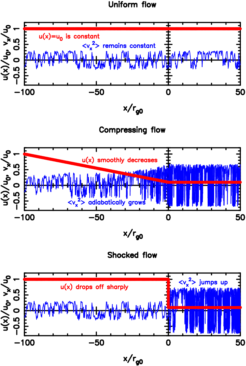
Figure 5 shows the results for these three cases. In the first case (top panel), with constant flow speed, varies with time in the range , with the average , but the dispersion remains constant. This case is similar to the situation studied in the previous test. In the second case (middle panel of Figure 5), where the flow speed linearly drops from to and then remains constant, we see a different behavior. The average particle motion is still locked with the plasma (), but the dispersion increases as drops. This means that the particle’s energy in the plasma frame grows. Such energizing of the particles is, in fact, the adiabatic heating of a gas put in a slowly shrinking volume (see Appendix B of [123] or Section 1.2 in [126]). In the third case (bottom panel of Figure 5), where the flow speed is constant at , but drops abruptly from to , similarly to what it looks like in a shock, the particle is energized significantly at the shock crossing. I, actually, had to introduce a reflecting boundary at that doesn’t allow the particles to cross the shock backwards, from to , in order to show a concise plot. Such crossing back becomes possible because the speed of the particle in the plasma frame is greater than the shock speed.
4 Calculating particle distribution and its moments
To calculate the particle distribution in the simulation, the simulation registers particles crossing certain locations, that we hereafter refer to as ‘grid planes’, because these locations also define the spatial grid, at the nodes of which all the quantities: , , etc., are defined. One may think of this as detection of particles by imaginary detectors placed at discrete locations upstream and downstream of the shock. This calculation may seem a bit tricky because each crossing of a detector by a particle contributes not to the density, but to the flux of particles, so in order to extract the particle distribution information, one needs to properly weight the detected information. However, this weighting is a standard procedure for simulations like ours, and below I demonstrate the reasoning leading to it and examples of the scheme at work.
The Monte Carlo simulation does not populate the whole space with particles; instead, it introduces particles upstream and propagates them one by one, until each leaves the system; yet, it is simulating a steady state solution with this process. This means that if one wants to calculate the particle distribution function and its moments (momentum and energy fluxes) at some spatial locations, one must collect the information about the particles in such a way that all the data collected in the course of one iteration (i.e., during the propagation of all the simulation particles) represents the information that would be collected by particle detectors placed in the plasma in a unit time (e.g., in one second).
The simulation only registers the particles’ contribution to when they cross one of the ‘detectors’. Consider an infinite plane detector in a spatially uniform plasma with no bulk motion () and an isotropic distribution of particle momenta; assume also that all particles have the same speed . Clearly, in a unit time such a detector will register more particles incident normally onto it than tangentially to its plane. It is easy to understand that the number of detected particles with a certain is proportional to , where is the x-component of the particle’s velocity in the rest frame of the detector and is the probability density of its detection in a unit time.
When a ‘detector’ in the simulation registers a particle with small , we must interpret it as that there are many similar particles at this location, but, because of an unfavorable direction of motion, only a few reach this parallel-plane detector in a unit time that one iteration represents.
Quantitatively, if one wants to calculate the number density of particles at the location of the detector, the code must compute the following sum:
| (7) |
where is the number of the grid plane, and – its coordinate, is the number density of particles at , and the summation index runs over all the events of a particle crossing this detector in the course of an iteration. The weight is the statistical weight of the -th event, and is the statistical weight of the particle participating in the event. The statistical weight of a particle, if particles are introduced upstream, representing a plasma density , is simply . The statistical weight of the event is expressed by the ratio , where the denominator is the -component of the particle velocity measured in the rest frame of the detector, at the -th event, and acts as the appropriate normalization factor.
If one wants to calculate the particle distribution function, i.e., the number of particles in a unit phase space volume , then the summation must be restricted to the events corresponding to that phase space volume. In practice, one may be interested in the distribution function such that
| (8) |
where represents the infinitesimal spherical angle corresponding to the momentum space volume . In the simulation, given a phase space binned so that is the width of the -th momentum bin centered at the momentum value , and averaging over the angles, one gets
| (9) |
where is the differential of the solid angle in -space, and the index runs over all particles whose momentum falls into the -th momentum bin. Indeed, with defined this way,
| (10) | |||||
as expected (in the summation, the index runs over all the momentum bins defined in the simulation, and in the last summation, runs over all the events of particle crossing of the detector). In the future, the plots showing actually show , but I omit the bar representing the angular averaging for simplicity.
Calculating the angle-averaged distribution function may be informative, but for practical purposes one needs the moments of the distribution function (i.e., the mass, momentum and density fluxes) that require the information about the angular dependence. From the above reasoning (namely, Equation 10) one may conclude that the correspondence between the integration over the momentum space and summation over particle detection events is as follows:
| (11) |
Therefore, for any function of coordinate and momenta , its expectation value may be calculated directly in the simulation as
| (12) |
Namely, for one finds the particle density, for – the mass flux in the -direction, for – the flux of the -component of momentum in the -direction, and for – the energy flux in the -direction ( is the relativistic kinetic energy corresponding to the momentum ). The expectation value of the function is the diffusive current , and in the case of isotropic momentum distribution gives the pressure.
| (13) | |||||
| (14) | |||||
| (15) | |||||
| (16) | |||||
| (17) | |||||
| (18) | |||||
| (19) |
etc. In the last two equations, the integration was limited to the thermal or to CR particles only. In this way I define the thermal pressure and the CR pressure. I must remind the reader here that a peculiarity of the approach I adopted is that in order to separate the CR particles from the thermal ones, the code uses their history, and not their energy. By my definition, a thermal particle is one that had been introduced into the simulation upstream with a random thermal energy and that may have crossed the subshock going downstream, but has never crossed it back. Once a particle crosses the subshock (the coordinate , to be more precise) in the upstream direction, it by my definition is injected and becomes a CR particle.
Let us note here that, assuming that the particle distribution is isotropic, the fluxes of energy and momentum can be expressed via gas pressure as
| (20) | |||||
| (21) |
where is the pressure and is the enthalpy of the particles. These are well known results of the kinetic theory of gases.
5 Introducing particles into the simulation
Theory
In order to start the Monte Carlo simulation of particle transport, we must introduce thermal particles far upstream, or close to the subshock (the latter method is described in Appendix B of [123]). This task has two components: generating a particle population with the proper energy distribution, and choosing the appropriate angular distribution for these particles.
We normally assume that the unshocked plasma is thermal and has a certain temperature (a typical cold interstellar plasma has K). In order to generate a thermal population, we randomly choose the momentum of every particle introduced into the simulation so that the resulting distribution is Maxwellian:
| (22) |
In order to accomplish this, consider the function such that is the fraction of the thermal particles with momenta in the interval , i.e.,
| (23) |
By substitution
| (24) |
using the identity , we find that has the following distribution function:
| (25) |
(here is the fraction of particles with momenta corresponding to the interval ). The latter is a Gamma distribution with parameter . To generate a quantity with the above distribution, one can use the following recipe:
| (26) |
Here is a random deviate with a uniform distribution in , and is a deviate the the normal (Gaussian) distribution with the mean equal to and the dispersion equal to . The above method was adopted from [37].
Test
I tested the implementation of this procedure, and verified the distribution function in the Monte Carlo simulation, and the test results are shown in Figure 6.

The code introduced particles into the simulation, assuming that their temperature is K, and the density cm-3. The thick line shows the desired Maxwellian distribution calculated according to Equation (22). The thin line shows the result of the detection of the introduced particles at some grid plane, as described in Section 4, according to Equation (9). The local deviations of the Monte Carlo result from the theoretical curve are statistical fluctuations, and these decrease for greater number of particles. Otherwise, the match is excellent, demonstrating the correct implementation of the introduction and the detection of particles in my code.
The angular distribution of momenta of the introduced particles is a major issue of concern for a simulation like ours, because it determines the rate of particle injection into the acceleration process. When the simulation introduces particles at the coordinate , it is replacing the dynamics of these particles upstream of with an analytic description, consequently it must distribute particles in -space at the way they would be distributed having traveled from far upstream and reaching for the first time. This is equivalent to calculating a -space distribution of particles incident on a fully absorbing boundary at after scattering in a non-uniform flow . This is easy to do analytically if all particles have a plasma frame speed less than the flow speed (because then all particles crossing position do it for the first and the last time), and fairly complicated otherwise (see Appendix B). Let us assume in further reasoning, which is justified as long as the local sonic Mach number at the introduction position is large.
The problem is now reduced to the following. We know how to designate an introduced particle’s momentum, . But how do we choose its direction, identified by the angle such that ? As was stated earlier, it is assumed that the angular distribution of momenta of the introduced thermal particles is isotropic in the plasma frame, and there is an overall drift speed superimposed over this motion in the plasma. Therefore, it may seem natural (but is incorrect) to just choose isotropically in the plasma frame, and then transform them into the shock frame. The correct solution must account for the fact that when these particles cross a grid plane, their flux must be ‘flux-weighted’ as seen in Equation (7), because the number of particles arriving at in a unit time is proportional to the cosine of the angle that their shock frame velocity makes with the -axis. This can be done by assuming a probability density of of as
| (27) |
Here , , and is the particle speed in the plasma frame chosen using a random number generator according to (26). The constant can be found from the normalization condition
| (28) |
as
| (29) |
so
| (30) |
In order to generate such a particle distribution, we use a random number uniformly distributed between and and calculate as a function of . The identity
| (31) |
and substitution of the uniform distribution
| (32) |
lead to:
| (33) |
which is where we can derive from. Substituting (30) into (33), we get
| (34) |
Note that, if we did not account for the flux weighting and just prepared an isotropic distribution of particles in the plasma frame and then transformed it into the shock frame, then instead of the prescription (34) we would use
| (35) |
which is incorrect, as I show below.
If properly implemented, the introduced particle population as detected by the grid plane detectors should have a uniform distribution of in the plasma frame, . This corresponds to isotropy of . Let us perform two tests to confirm that the procedure (34) gives the correct particle distribution isotropic in the plasma frame.
In the first test, let us introduce particles into the simulation with a supersonic flow (sonic Mach number ) using the incorrect recipe (35). At the grid plane very close to the introduction position, the model will measure the angular distribution of particles, . Several (approximately 20) diffusion lengths downstream of the introduction position, it will measure again. By the time of the second measurement, the particles must have scattered enough to assume an isotropic velocity distribution in the plasma frame corresponding to . The results of the test are shown in Figure 8.


As expected, the thick line in Figure 8 is , meaning that after many scatterings, particles isotropize their velocities, and also confirming that I implemented correctly the calculation of particle distribution and the pitch angle scattering routine. At the same time, the tilt of the thin line tells us that the introduced particle distribution was not isotropic in the plasma frame, thus the recipe (35) is incorrect.
In the second test, particles will be introduced, now using the recipe (34) to choose their angular distribution. Let the model measure the angular distribution immediately, and some distance downstream of the introduction position. The results are shown in Figure 8. The two angular distributions match exactly, which means that the introduced angular distribution was isotropic, and remained such after many scatterings.
These tests conclude the verification of particle propagation methods of Monte Carlo, and now we can get to testing the particle acceleration properties.
6 Test particle case of DSA
A crucial test that the nonlinear simulation of DSA must pass is the production of a power-law spectrum of accelerated particle in the test particle case. Similarly to the solution shown in Section 5, a shock characterized by a sharp transition at , in which the flow speed jumps from the to , with a compression ratio and particle injection taking place at the shock via thermal leakage, must produce a power-law spectrum of accelerated particles with the power law index given by Equation (23). Verifying the power law index is a strong argument for the correctness of the model.
We ran 3 simulations with a discontinuous flow speed. In each simulation, km s-1, K, cm-3, and to define the mean free path, the model assumed Bohm scattering in a magnetic field G (see Section 1). The difference between the 3 models was the compression ratio, . I chose for the first model, for the second and for the third. Note that I did not require consistency of these compression ratios with the laws of hydrodynamics, and was only interested in particle acceleration and its properties. Namely, according to Equation (23), one expects to get power-law distributions of accelerated particles downstream with the indices , and , for the first, second and the third model, respectively. In these runs I took advantage of the procedure of particle introduction developed in Section 5 and introduced particles close to the shock instead of far upstream. This allowed us to speed up the calculation significantly, and thus I put the free escape boundary rather far upstream, at .

The results of the test – the particle distributions measured in the shock rest frame – are shown in Figure 9. The solid lines are the particle distributions in the shock frame measured in the downstream region. The -axis shows proton momentum in units of , and the -axis – the distribution function multiplied by for convenience. This multiplication factor makes the case with the corresponding appear as a horizontal line, which is a desirable feature of this plot. In the future, all particle distribution functions shown will have this multiplication factor. The thin solid line shows the detected distribution function for , the medium thickness solid line – for and the thick solid line – for case. The dashed lines are added for a comparison. They have the slopes predicted by Equation (23), and for the correct result, the dashed lines must be parallel to the high-energy parts of the distribution functions, which is certainly the case in the presented results.
I would also like to illustrate the physical process that leads to particle acceleration in these tests. In a separate simulation similar to the case, but with a free escape boundary close to the shock, at , the code traced several particles, and I show their motion in the phase space in Figure 10

The top panel of Figure 10 shows the shocked flow speed. Upstream, at , the flow is uniform and fast, km s-1, and at the shock located at , the flow speed drops down to . This flow speed is measured in the system where the shock is stationary, so the flow of matter is directed from the left end to the right end of the plot, and the shock is directed to the left.
The second panel shows a particle introduced far upstream, that crossed the shock, got heated, but never returned upstream and escaped trapped in the downstream flow (the particle’s motion is from the left to the right end of the plot). This is what happens to all particles in collisional shocks that are usually observed on Earth, and no particle acceleration occurs.
The third panel shows a particle initially introduced far upstream as a thermal particle, but its random motion in the stochastic magnetic fields, induced by the pitch angle scattering, lead the particle back upstream, and it crossed the shock from the region into the region. In several such subsequent crossings, the particle gained energy due to the flow speed difference across (the trajectory moved up). Eventually this particle’s energy became so large that it was able to protrude quite far upstream, to , but eventually it was advected downstream with the flow.
The fourth (bottom) panel in Figure 10 shows the phase space trajectory of a ‘lucky’ particle that not only got injected (crossed the shock against the flow), but gained enough energy to find itself very far upstream, to the left of the free escape boundary located at . There such particles were assumed to escape from the system in the upstream direction – this is how the finite size of the accelerator is modeled in the Monte Carlo simulation. The energy of this particle at the moment of escape was close to the maximum achievable particle energy in this shock. The particle’s speed greatly exceeded the shock speed at this moment, with the particle actually being mildly relativistic . In a model representing a real SNR shock, the free escape boundary would have been located much farther upstream, and particles would be able to make many more crossings before escaping upstream, and the maximum particle momenta could be ultrarelativistic, .
7 Shock compression ratio in nonlinear DSA
Theory
In a standard steady state hydrodynamic shock, the relationship between the pre-shock macroscopic quantities: , , and their post-shock values: , , is determined by the sonic Mach number of the shock, and can be derived from the Rankine-Hugoniot equations:
| (36) | |||||
| (37) | |||||
| (38) |
which express the conservation of mass, momentum and energy fluxes, respectively. Here is the gas pressure, and – its enthalpy, , and the internal energy of the gas is proportional to the pressure . For an adiabatic gas with the ratio of specific heats , one can write , and the upstream gas pressure can be related to the sonic Mach number as . This leads to a solution of the Rankine-Hugoniot equations, relating the pre-shock and the post-shock flow speed and temperature. That solution is called the Hugoniot adiabat:
| (39) | |||||
| (40) |
where is the compression ratio22 2 Hereafter let us replace the notation of the total shock compression ratio. Instead of , we will now denote it as , to distinguish it from the subshock compression ..
In a nonlinear shock with magnetic field amplification, the situation is complicated by the contributions of cosmic ray pressure and magnetic turbulence pressure, and by particle escape far upstream. The procedure of the search of the self-consistent compression ratio, developed in [43], is based on the requirement that in a steady-state system, mass, momentum and energy fluxes must be constant in space. I generalized this procedure for the problem of magnetic field amplification by including the contributions of magnetic turbulence to the conservation relations, and developed an iterative procedure for an automated search of the self-consistent . Consider the conservation relations
| (41) | |||||
| (42) | |||||
| (43) |
Here and are the mass density and the flow speed, is the flux of the -component of momentum in the -direction including the contributions from particles and turbulence, and is the far upstream value of momentum flux, i.e.,
| (44) |
The quantity is defined as
| (45) |
where and are the -components of momentum and velocity of particles, and is their distribution function, all measured in the shock frame. The quantity is the energy flux of particles and turbulence in the -direction, is the energy flux of escaping particles at the FEB,33 3 Particle escape at an upstream FEB also causes the mass and momentum fluxes to change but these changes are negligible as long as (see [43]). and the far upstream value of the energy flux is
| (46) |
The quantity is defined as
| (47) |
being the kinetic energy of a particle with momentum measured in the shock frame. and are the momentum and energy fluxes of the turbulence defined in Section 9.
Writing equations (41), (42) and (43) for a point downstream of the shock, sufficiently far from it that the distribution of particle momenta is isotropic, and the approximations (20) and (21) are valid, and denoting the corresponding quantities by index ‘2’, we get the equivalent of the Rankine-Hugoniot relations, that accounts for particle acceleration and escape, and for the presence of magnetic turbulence:
| (48) | |||||
| (49) | |||||
| (50) |
The particle gas enthalpy is , and the internal energy of gas is proportional to the pressure . Introducing the quantity so that , one can write
| (51) |
The value of is averaged over the whole particle spectrum, and it ranges between for a nonrelativistic and for an ultra-relativistic gas. The local value of can be easily calculated in our code from the particle distribution, along with and , as . Similarly, one can define and calculate a local value of anywhere in the code in order to express
| (52) |
The value of depends on the nature of the turbulence. For instance, in Alfvénic turbulence, one expects , [see Equation (185)].
Substituting (51) and (52) into the above equations and introducing , we can eliminate using (48) and using (49), which allows us to express from (50) the quantity as
| (53) |
where
| (54) | |||||
| (55) | |||||
| (56) |
Note that , where due to the absence of CRs far upstream. The pressure of stochastic magnetic fields can be found from the spectrum of seed turbulence far upstream (see Section 2).
The quantity is readily available in the simulation after the end of any iteration. Comparing it to the value predicted by (53), one may evaluate the self-consistency of the solution and make the correction to , if necessary, for further iterations. For making these corrections it is helpful to use in the simulation the inverse of (53), the physically relevant branch of which is
| (57) |
It is important to emphasize here that an iterative procedure is required to find the compression ratio of a non-linearly modified shock, because quantities , and depend on , so (57) only provides a practical way to perform the iterations. The code employs the following procedure:
| (58) |
where is a small number (typically ). Here is the compression ratio assumed for the last iteration, and – the compression ratio chosen for the following iteration. The weighting using the parameter is chosen so that, when the deviation of the nonlinear structure of the shock from the self-consistent solution is large, this iterative procedure would not overcompensate the discrepancy, which may lead to the breakdown of the model (for example, is unphysical, and too high may stall the particle transport procedure).
Another complication that may arise with the procedure described by (58) is that instead of converging to a solution that satisfies the conservation relations (48), (49) and (50), the procedure may find an attracting cycle around the self-consistent value of . For example, may be too low in one iteration, underestimating particle acceleration efficiency, which leads to a shock with a high predicted by (58). The latter, in turn, overestimates particle acceleration, leading to a low compensatory prediction again. These cycles may be merely a mathematical consequence of our numerical model of particle accelerating shocks. On the other hand, it is conceivable that a real shock, instead of evolving into a steady-state system, may behave periodically or even chaotically, turning particle acceleration on and off. However, these effects are beyond the scope of the present research, because we look for the steady-state structure of collisionless shocks. The simulation avoids the attractors other than the self-consistent solution by randomizing the value of , so that it varies between a finite value and in every iteration. This way, any attracting cycle that the system (58) may have with a constant value of will eventually be broken, but if is at its self-consistent value (), the randomization of will not take the solution away from this point. The latter is expected as long as statistical fluctuations of quantities , , and keep in the attracting domain. This only requires that a high enough number of particles is used in the Monte Carlo routine.
Test of the implementation
We test the procedure of the iterative estimation of the compression ratio (58) by confirming that it reproduces the solid predictions of the Hugoniot adiabat (39) and (40). In 10 runs described below, the shocks propagate in a gas with density cm-3, temperature K (corresponding to a sound speed km s-1), and magnetic field G determining the Bohm diffusion (this magnetic field is too small to influence the momentum and energy balance, therefore the Hugoniot adiabat should apply). I performed 9 runs, in which the flow speed, , varied from km s-1 to km s-1, corresponding to the sonic Mach number, , varying from to . In these simulations, I artificially eliminated particle acceleration by assuming that the subshock is fully reflective for particles trying to cross it from the downstream into the upstream region. Additionally, I ran simulation number 10, for which the subshock is assumed fully transparent, and particle acceleration occurs (limited by a free escape boundary at ). We start the simulations off by assuming a flow with the speed , which at the point abruptly slows down by to . This tiny flow speed jump heats the particles a little, just enough to make the procedure (58) start converging to a self-consistent . Setting the parameter and randomizing it between and , in iterations the simulation obtains the self-consistent value of . I averaged the prediction over the last iterations out of , and showed the results in Table 1. Additionally, the simulation measured the downstream gas temperature, , by detecting thermal particle pressure and relating it to the temperature by the ideal gas law.
lccccccc Model , km/s Accel. – MC
1 5 0.5 no 1.0* 1.022 0.003 1.0* 0.99 0.08
2 10 1.0 no 1.0 1.05 0.01 1.0 1.02 0.05
3 12 1.2 no 1.30 1.31 0.02 1.19 1.19 0.06
4 15 1.5 no 1.71 1.73 0.01 1.49 1.48 0.06
5 20 2.0 no 2.29 2.29 0.01 2.08 2.0 0.1
6 30 3.0 no 3.00 2.99 0.01 3.67 3.7 0.1
7 50 5.0 no 3.57 3.58 0.02 8.68 8.4 0.3
8 100 10 no 3.88 3.90 0.01 32.1 31 1
9 300 30 no 3.99 4.00 0.01 282 290 10
10 300 30 yes 3.99** 3.11 0.09 282** 230 10
Column ‘Model’ in Table 1 shows the number of the model, is the upstream flow speed, – the corresponding Mach number, ‘Accel.’ shows whether the Fermi-I acceleration was allowed, as described above. The columns ‘’ and ‘’ are the predictions of the Hugoniot adiabat (39) and (40) corresponding to the Mach number and the adiabatic index of a non-relativistic ideal gas . The columns ‘’ and ‘’ show the result of the simulation, i.e., the average of the last of the iterations, along with the standard deviation. For , the Hugoniot adiabat doesn’t apply, because the flow is subsonic, and no shock should form, corresponding to and (values marked with the asterisk ‘*’).
It is clear that, within statistical errors, the simulation n Models 1-9 reproduced the Hugoniot adiabat results for nonrelativistic hydrodynamic shocks. Note that the physics that the simulation is based on at this point involves only the isotropic particle scattering, the Lorentz transformations between the reference frame of the flow and that of the shock, and the requirement that the calculated momentum, energy and mass fluxes be conserved.

Figure 11 illustrates how the prediction of the self-consistent compression ratio for Model 9 starts off with a trivial initial guess of , rises up to the value predicted by the Hugoniot adiabat in 15 iterations, and stays there.

Figure 12 confirms the conservation of momentum and energy across the shock in Model 9. The top panel shows the flow speed with the compression ratio , the middle panel shows the momentum flux measured in the units of the upstream flux, and the bottom panel shows the energy flux. These fluxes remain constant throughout the shock for Model 9 (the dashed thick line).
Now let’s analyze the results for Model 10, which is the same as Model 9, but with the shock transparent to the particles, so that the process of diffusive shock acceleration can occur. The Hugoniot adiabate is not applicable in this case, and the corresponding values in Table 1 are marked with a double asterisk ‘**’. Indeed, the values of the compression ratio and the downstream temperature determined by the simulation and shown in Table 1 are , and . These values are is lower than the prediction of the Hugoniot adiabat for a shock with the sonic Mach number . In Figure 11, the thick solid line demonstrates that the iterative procedure given by Equation (58) has converged, but the fluxes shown with the solid lines in Figure 12 are not constant, meaning that the derived solution is not physical. This is the effect of particle acceleration studied by Ellison and co-workers using the Monte Carlo model, and the commonly accepted solution is that a shock precursor must form, i.e., the upstream flow speed must decrease towards the shock. The procedure that models it is demonstrated in Section 8.
8 Nonlinear structure of the shock precursor
Theory
In the test-particle limit, the aftermath of particle acceleration by a shock with the compression ratio is the power law spectrum of accelerated particles every point in space, . The power law index of the spectrum for a strong shock with is , which has the unphysical property that, if it were to stretch from to , the pressure (and the internal energy) of the particles with such a spectrum, , would logarithmically diverge at the high momentum end. In reality, of course, the spectrum is limited by the maximum momentum determined by the size of the shock or the acceleration time. However, the logarithmic divergence of pressure at high energies means that there may be a large amount of energy in the highest momentum particles. Of course, the actual amount of energy is determined by the rate of particle injection.
Initially, the shock in the simulation doesn’t have a self-consistent structure because it starts with an unmodified shock and is overestimated at all locations where accelerated particles are present (see, e.g., the plots for Model 10 in Figure 12). Therefore, it must choose to reduce the mismatch between the local momentum flux and the far upstream value of it for , as described by Equation (42). It can be done by calculating
| (59) |
where is the predicted flow speed for the next iteration, and is a small positive number (typically around 0.1), characterizing the pace of the iterative procedure. The value of the parameter is randomly chosen between and a finite value for reasons similar to those described in Section 7. If magnetic field amplification is invoked, then at this point the simulation also refines its estimate for the particle diffusion coefficient (see Section 3).
The predicted and are then used in a new iteration where particles are injected and propagated. The calculated CR pressure, momentum flux, etc. are then used to refine the guesses for and for the next iteration, along with the guess for the compression ration . This procedure is continued until all quantities converge.
Test of implementation
In order to test the implementation and the effects of the precursor smoothing, I complemented Model 10 with the procedure (59). I had to reduce the maximum value of from to and make many more iterations in order to restrict the self-consistent compression ratio . As Figure 13 shows, the iterative procedure converged to a value , much higher than the Hugoniot adiabat predicted44 4 This and other nonlinear effects are discussed in [43]..

In Figure 14, I show the spatial structure of the smoothed shock. In the top panel, a reduction of the flow speed from in the upstream region, , is apparent. Let us refer to the smoothed region as a shock precursor. A subshock at has a compression ratio, . Momentum flux shown in the second panel is conserved within a few percent, and its deviation from conservation is statistical (the shown plots are an average of 14 iterations at the end of the 500 iterations leading to a consistent solution). The energy flux (third panel from top) drops at the upstream free escape boundary, , by 60%, which is explained by particle escape. Downstream of the free escape boundary, the energy flux is almost constant (within statistical deviations). The thin dashed line in this panel shows the self-consistent value of energy flux accounting for particle escape, as determined by equation (53); as one can see, the actual value of is in excellent agreement with this quantity. The bottom panel shows the constituents of the momentum flux , the dynamic pressure , the thermal particle pressure and the cosmic ray pressure . One can easily see that the shock is dominated by the accelerated particles in this case.

9 Summary
I would like to conclude this lengthy section with a summary. The simulation of nonlinear shock acceleration presented here features a Monte Carlo code of particle transport and an iterative procedure for deriving a self-consistent shock structure.
The tests I presented here confirm that:
- •
Particle propagation simulated by the Monte Carlo method is diffusive, and that it reproduces qualitatively and quantitatively the expected behavior of such particle transport;
- •
The simulation reproduces the well-known results for hydrodynamic shocks (i.e., the Hugoniot adiabat), if particle acceleration is artificially blocked;
- •
Accelerated particle spectra predicted by the simulation in the test-particle regime agree with the solid predictions of analytic models of test-particle acceleration;
- •
When the feedback of accelerated particles in the nonlinear regime is accounted for, the simulation obtains a stable solution that conforms with mass, momentum and energy conservation laws.
The methods of the Monte Carlo simulation of particle transport and the idea of iterative derivation of nonlinear shock structure presented here are not original to this dissertation, they were developed by Ellison and co-workers. I will not elaborate any more on the subject of nonlinear shock acceleration and refer the reader to the literature for more information (e.g., [72] and [92]).
The original part of the model – magnetic field amplification and self-consistent particle transport – will be presented in the rest of this Chapter. The reason I presented and tested the Monte Carlo part of the model in such detail is that the actual computer code used in the research was written by the author of this dissertation and had to be tested to confirm that it reproduces the well known, previously established results. Besides that, some details of the currently employed methods did not appear in our publications, and I would like to make a record of these details here.
2 Magnetic Field Amplification
In this section I will describe two theoretical models of magnetic turbulence amplification by streaming particles available in the modern scientific literature. Then I will proceed with a generalization of these models for the problem of nonlinear DSA, and present the analytic description of magnetic field amplification adopted for the model, and its numerical solution. I will conclude by describing the feedback of the amplified magnetic turbulence on the plasma flow.
The physical conditions in which the instabilities take place are representative of the conditions in a collisionless shock precursor. A fully ionized plasma is moving at a speed from the far upstream, unshocked region () towards the subshock located at , where it gets non-adiabatically compressed. We assume that a pre-existing uniform magnetic field parallel to the plasma flow fills the space. The instabilities are induced by the accelerated particles produced by diffusive shock acceleration, and described by . These particles are subject to diffusion in the plasma and advection along with it. Therefore, in the reference frame locally co-moving with the plasma, the CRs appear to move against the bulk flow, away from the subshock. The CR density and pressure increase from at to a finite value at , and so does the diffusive current of CR measured in the plasma reference frame55 5 Speaking of CR current and CRs streaming, I will always mean the apparent drift of CRs in the plasma reference frame..
We describe the fluctuations of magnetic field in the plasma by the energy spectrum of turbulence, . The latter is a quantity such that is the volume density of turbulent energy (i.e., the energy of the waves, including the magnetic field energy and that of the associated stochastic plasma motions) in the waveband . This means that, instead of the the spatial structure of the turbulent magnetic fields, the simulation only follows the evolution of its Fourier transform, locally calculated over a large enough volume, and averaged over a large enough time interval. This approach relieves our model from the computational expenditure of PIC plasma simulations, because the latter have to have a spatial resolution finer than the size of the smallest turbulent vortex, while our simulation gets away with a resolution that is more coarse than the largest turbulent harmonic by describing the processes on smaller scales statistically. Obviously, this advantage is gained at the cost of having to rely on theoretical models of processes in plasmas instead of performing a numerical experiment based on more fundamental physical principles.
Magnetic turbulence amplification is modeled under the assumption of a steady state situation, i.e., the time derivatives in the respective equations are set to . It is also postulated that in the interstellar medium (i.e., far upstream), there exists seed turbulence, which is expressed by the boundary condition
| (60) |
Expression (60) describes a far upstream seed turbulence with a power law spectrum, , normalized so that , where is a parameter of the model representing the assumed effective magnetic field of the seed turbulence. The values and limiting the wavenumber range of the seed turbulence spectrum are also parameters of the model. Normally, the code will choose them so that for particles of all energies found in the simulation, the resonant wavenumber (defined later) is between and .
The effective magnetic field at any point is a quantity that I define as
| (61) |
The fraction before the integral in the right-hand side of Equation (61) expresses the assumption that one half of the turbulence energy is contained in the magnetic field fluctutaions, and the other half is carried by the stochastic fluctuations of the plasma velocity associated with the waves. The factor is exactly correct when the turbulence is purely Alfvénic (see Section 9). The expression (61) is therefore a good approximation if the turbulence is generated by the resonant streaming instability (see Section 1), but does not apply, for example, to the waves generated by the nonresonant Bell’s instability (see Section 2). For the latter case, the relationship between the plasma velocity fluctuations, , and the magnetic field fluctuations, , can be inferred, for example, from Equation (17) in [10]. It can be shown that for wavelengths at the peak of the amplification rate, (defined in Section 2) magnetic field contains , and velocity fluctuations – of the total energy density . However, I use the ‘50/50’ distribution of the turbulent energy between magnetic and kinetic fluctuations, expressed by the factor in Equation (61), for turbulence produced by any source. I do so for the following reasons. First, considering the much larger uncertainties in some other factors of the model (e.g., the diffusion coefficient), an adjustment of the expression (61) to account for the nature of the turbulence would be a minor correction. Second, nonlinear turbulent processes like dissipation and cascading may change the energy distribution between magnetic and velocity fluctuations, and there exists no analytic description of this process adequate for the strong turbulence considered in this model.
1 Resonant cosmic ray streaming instability
Charged particles streaming along a uniform magnetic field are able to resonantly amplify Alfvén waves traveling along the same field ([81, 118, 126, 9], etc.). The mechanism of Alfvén wave amplification is similar to that used to amplify electromagnetic waves in the electronic device known as the traveling-wave tube [63]. Alfvén waves exchange energy with fast particles of resonant momenta. If the particle distribution is anisotropic, Alfvén waves traveling in one direction get amplified, and waves traveling in the opposite direction get dampened by the interactions with the particles close to the resonance. I will not describe this instability in detail and refer the reader to the sources cited above.
Assuming a steady state and that the particle distribution is controlled by advection of the flow and resonant turbulent diffusion (see Section 2), and that the generated waves are a weak perturbation of the uniform magnetic field, , the evolution of may be described (see [82] and references therein) as
| (62) |
if all other effects accompanying wave generation are ignored. Here the growth rate
| (63) |
and
| (64) |
defines the resonant momentum, . Here is the Alfvén wave speed, and is the spectrum of particle pressure, normalized so that is the pressure of accelerated particles in the momentum range .
It was usually assumed that the fluctuations grow until , after which the instability saturates (e.g., [93]). Recently, Bell and Lucek [11] suggested that, if the instability can grow beyond this point, to , the observations of large magnetic fields in some SNRs can be explained by generation of magnetic fields in the process of DSA. Simulations done by the same authors [86] support such a possibility. Here, I adopt Bell and Lucek’s idea and assume that the streaming of CRs is able to produce strong magnetic field fluctuations.
As the perturbations grow and reach , however, it is likely that waves with wave vectors not aligned with will be generated, due to local CR pressure gradients along the total . With , it becomes impossible to predict the average value of the transverse pressure gradients and the resulting magnetic field structure without knowing the relative phases of different wave harmonics. The problem is further complicated by the fact that this longitudinal, compressible turbulence may produce a strong 2nd order Fermi particle acceleration effect which, in turn, can damp the longitudinal fluctuations (see, for example, [105]).
These complications place a precise description of plasma turbulence beyond current analytic capabilities. However, valuable conclusions about MFA in efficient DSA can be made by considering the two limiting cases of the resonant instability development in the nonlinear regime. The first assumes there is no longitudinal turbulence, in which case the wave growth rate is determined by the Alfvén speed in the non-amplified field . This gives a lower bound to the growth rate. The upper limit assumes that the turbulence is isotropic, in which case the growth rate is determined by the Alfvén speed in the much larger amplified field (defined in Equation (61)). The real situation should lie between these two cases, and while I consider these limits, I do not explicitly include second-order Fermi acceleration in the calculations. Section 1 describes the parameterization of the growth rate of the resonant instability that encompasses the minimum and the maximum growth rate in the regime of strong fluctuations.
2 Bell’s nonresonant instability
A nonresonant instability, theoretically described by Bell in 2004 ([10]), occurs when a strong external electric current of CRs is put through the plasma. The instability develops because the thermal plasma must provide a current in response to the external current of streaming CRs, in order to maintain quasi-neutrality. This current makes certain MHD modes unstable; these modes can be described as driven circularly polarized Alfvén waves. Again, I will not discuss the details of the instability; the reader may find more information in [10, 130, 4].
In the linear regime () the growth of the unstable modes can be described by the following equation:
| (65) |
The dispersion relation of waves subject to Bell’s instability is
| (66) |
where and are the frequency and the wavenumber of the generated waves, and is the diffusive current of CRs directed along the magnetic field . The frequency has an imaginary part when
| (67) |
and the reasoning leading to (66) is applicable when the wavelengths of the generated waves are shorter than the smallest energetic particle gyroradius in the system, :
| (68) |
Along with its applicability conditions (67) and (68), the growth rate of the energy of the waves is
| (69) |
Here is the Alfvén speed, and the critical wavenumber is
| (70) |
This instability has been studied theoretically and using MHD and PIC simulations ([10, 130, 5, 4, 104]), which show that it is capable of generating large magnetic fields, and may even dominate the resonant CR streaming instability in young shocks of SNRs [99].
It is informative for future reasoning to point out the dependence of on : the rate becomes non-zero at large wavelengths at , and then grows as towards the smaller wavelengths, until it peaks at , and then rapidly falls off down to zero at .
3 Nonresonant long-wavelength instability
Other instabilities possibly leading to magnetic field amplification may exist in an interstellar plasma in vicinity of a particle accelerating shock. Bykov and Toptygin [30] suggested a model in which streaming cosmic rays may amplify waves in plasma with wavelengths much larger than the gyroradii of the particles.
The model presented in [30] requires the presence of a neutral component in the plasma (i.e., unionized hydrogen atoms) that suppresses the transverse conductivity. The Balmer series lines of neutral hydrogen have been observed in the emission spectra of forward shocks of Type Ia SNRs (e.g., in SN 1006 and Tycho’s SNR [77]. See also the references in [60]). It is also possible that short-scale turbulence may act similarly to neutral plasma component at suppressing the transverse conductivity, which will make the model of nonresonant long-wavelength instability applicable to fully ionized plasmas as well (A. M. Bykov, in private communication, and [27], in press).
I have not incorporated this effect into the simulation, because the details of this model are being developed. However, if this instability operates in the precursor of a collisionless shock, it may have a very strong impact on the maximum momentum of the accelerated particles due to its long-wavelength nature.
4 Evolution of turbulence in a nonlinear shock – other effects
Flow compression
Equations of the form (62) and (65) generally apply to a uniform flow , and do not take into account the possibility of a changing flow speed in the precursor. In the geometric optics approximation, the propagation of waves in a medium with changing properties may lead to modulation of the wavelengths and of the amplitudes of the waves. Different instabilities generate different types of waves, which may evolve differently. Namely, the resonant CR streaming instability in the quasi-linear approximation generates Alfvén waves propagating against the flow, and Bell’s nonresonant instability generates almost purely growing harmonics that can be described as driven Alfvén waves [10]. Considering that compression ratios in strong SNR may reach (see, e.g, observational arguments [125, 33], and theoretical predictions [72, 92]), these effects may change the wavelengths and amplitudes of the generated waves by a large factor, and should be considered.
I propose to include the effects of flow compression in the model by adding the corresponding terms to the equation of turbulence evolution. Consider the equation
| (71) |
Given a boundary condition , one can readily solve this equation for using the method of characteristics: see Equation (104). The ratio in this equation is the factor by which the plasma is compressed, because due to Equation (41), . Equation (104) shows that the parameter determines how the amplitudes of the waves react to compression, namely, . For Alfvén waves, the correct value of this parameter is (see the wave generation equations and the corresponding explanation in [122]). The parameter describes what happens to the wavenumber of the waves as they propagate in the compressing medium, that is, .
Dissipation
The amplified turbulence may be dissipated through collisional and/or collisionless mechanisms and these include: (i) linear and nonlinear Landau damping (e.g., [1, 80, 120, 128]), (ii) particle trapping (e.g., [94]), and (iii) ion-neutral wave damping (e.g, [39, 30]). Existing analytic descriptions of MHD wave damping rely on the quasi-linear approximation , which is inapplicable for strong turbulence, and numerical models with varying ranges of applicability have been proposed which offer a compromise between completeness and speed (e.g., [10, 3, 122, 130]). Because no consistent analytic description of magnetic turbulence generation with exists, and because an numerical (MHD or PIC) description of this process in the framework of non-linear DSA is very computationally expensive, we propose a parameterization of the turbulence damping rate. In doing this, we are pursuing two goals. First, we make some predictions connecting cosmic ray spectra, turbulent magnetic fields and plasma temperatures, which, in principle, can be tested against high resolution X-ray observations in order to estimate the heating of the thermal gas by turbulence dissipation. And second, once heating is included in our simulation in a parameterized fashion, we will be ready to implement more realistic models of turbulence generation and dissipation as they are developed.
The heating of the precursor plasma by dissipation modifies the subshock Mach number (e.g., [44, 123]) and this in turn modifies injection. The overall acceleration efficiency and, of particular importance for X-ray observations, the temperature of the shocked plasma (e.g., [36, 69, 54]) will depend on wave dissipation.
The generalized way of including the dissipation of turbulence into the simulation is introducing a corresponding term into the equation of turbulence evolution:
| (72) |
where stands for the rate of growth of the instability driving the turbulence (i.e., ), and is the rate of turbulence dissipation (measured in ergscm-3s-1). In the simulation, I allow for one of two prescriptions for the dissipation rate to be realized.
In the absence of a better model, one may assume that the dissipation rate is proportional to the amplification rate , i.e.
| (73) |
where is a number between and . Equation (73) is a mere parameterization of the dissipation rate, in which is the fraction of the instability generation rate that is assumed to go directly into particle heating rather than magnetic fields (in , the subscript stands for ‘fraction’). In particular, corresponds to no dissipation, and describes a situation where all the turbulence generated by a particle streaming instability immediately gets dissipated and transformed into heat.
Another prescription for the rate of dissipation is
| (74) |
The wavenumber at which the dissipation begins to dominate, , is identified with the inverse of a thermal proton gyroradius:
| (75) |
where is the proton mass, is the Boltzmann constant and is the local gas temperature. This prescription is a relaxation-time approximation, defined in such a way that at , the dissipation time equals the period of an Alfvén wave with the wavenumber , and the -dependence is . The dependence of the dissipation rate is based on the assumption that viscosity (i.e., magnetic viscosity in this case) drives the dissipation (see, e.g., [120]).
Influence of turbulence dissipation on thermal plasma heating
Dissipation of turbulence acts as an energy sink, in which the magnetic and kinetic energy of turbulent fluctuations are transformed into the internal energy of the thermal particle gas. This means that, in order to conserve energy, the appearance of the term in the equation of turbulence evolution must be accompanied by the corresponding correction to the equations of motion of the thermal plasma. The way to incorporate the thermal plasma heating due to turbulence dissipation was shown in [93], who derived the equation of thermal pressure evolution in the shock precursor:
| (76) |
Here the ratio of specific heats of an ideal nonrelativistic gas is . For , equation (76) reduces to the adiabatic heating law, and, for a non-zero , it describes the heating of the thermal plasma in the shock precursor due to the dissipation of magnetic turbulence. The fluid description of heating given by equation (76), while it doesn’t include details of individual particle scattering, can be used in the Monte Carlo simulation to replace particle scattering and determine heating in the shock precursor. This merging of analytic and Monte Carlo techniques, or Analytic Precursor Approximation (APA), is described in detail in Appendix B of [123], and briefly summarized below.
When the heating rate, , becomes available from the solution of the turbulence growth equation (86), the code solves (76) and substitutes the solution, , for the thermal pressure calculated from particle trajectories. It is done in the upstream region up to the point , at which thermal particles are subsequently introduced into the simulation for the next iteration. In order to include the effects of heating in the model, we must introduce thermal particles at as if they were heated in the precursor, i.e., their temperature must be determined by (76) and the ideal gas law:
| (77) |
The simulation therefore chooses the magnitude of every introduced particle’s momentum in the local plasma frame distributed according to Maxwell-Boltzmann distribution with temperature determined by (77) at . As long as the local sonic Mach number at this location is large (i.e., ), it can be done using the results of the section 5 for the angular distribution of the introduced particles. If the (which does not usually happen in a self consistent solution), then the results described in Appendix B may be applicable.
Spectral energy transfer
Observations of turbulence, including the MHD turbulence in the interplanetary plasma, often report spectra that look like power law functions of over many decades. This phenomenon can successfully be explained by spectral energy transfer (cascading). After the energy has been generated by an instability on some dominant spatial scale, nonlinear motions in the turbulent fluid cause splitting and merging of the turbulent vortices (i.e., a cascade), leading to a re-distribution of energy between different scales. This way, turbulence initiated by large-scale vortex formation due to an external power source can cascade into smaller vortices, producing a power-law distribution of energy in the so-called inertial range (i.e., the interval in -space where the turbulence spectrum is populated by cascading rather than directly by the instability). This cascade continues until the size of the vortices is small enough so that dissipation [e.g., (74)] terminates it by converting the energy of motion into heat in the so-called dissipative region of -space (e.g., [17]).
There are various ways to describe spectral energy transfer (see, e.g., [96]). One of the simplest methods, listed in [96] as the Kovazhny hypothesis, involves a dimensional analysis argument. If one writes the equation of turbulence evolution in the inertial range as
| (78) |
then by the physical meaning, is the flux of energy through -space towards larger . Assuming that is a product of powers of the minimum set of relevant quantities, one can find the simplest form of the corresponding cascading rate. That is, if , then the only combination of , and that gives the correct units is
| (79) |
As we will see later, this cascading rate gives a stationary solution , which is known as the Kolmogorov spectrum, and the corresponding cascade will be referred to as Kolmogorov-type cascade (here denoted by the subscript ‘K’).
When MHD turbulence is considered, the simple dimensional argument shown above does not work because the magnetic field is another relevant quantity. There are two approaches to describing nonlinear effects (spectral energy transfer) in MHD turbulence. One, proposed by Iroshnikov and, independently, by Kraichnan [70, 78], treats the MHD turbulence as weakly interacting plasma waves that can undergo mergers and splitting. The bottom line of this approach is that a stationary spectrum is predicted. Because and are so close, it is difficult to distinguish between the two indices in the analysis of observations. Goldreich and Sridhar [64] point out that the MHD turbulence is inherently anisotropic (even if there is no mean magnetic field, the effective field of the large scale harmonics can play its role for the processes in the inertial interval), and the weak-turbulence approach is not applicable. These authors proposed another theoretical approach: they suggested a certain anisotropic damping rate and postulated a critical balanced state, which allowed them to derive an anisotropic turbulence spectrum. Their results predict that harmonics with wavevectors transverse to the uniform magnetic field experience a Kolmogorov-like cascade, while the cascade in wavevectors parallel to the field is suppressed. The waves generated with streaming instabilities are transverse; therefore the diffusion coefficient for particle transport parallel to the flow depends on the wavenumbers parallel to the magnetic field. Biskamp [17] shows that the Goldreich-Sridhar spectrum for parallel wavenumbers may be expressed as .
We can find the corresponding cascading rate, such that , which would lead to a steady state spectrum with . From the dimensional argument,
| (80) |
One may do a simple estimate and compare the Kolmogorov and the Goldreich-Sridhar cascading rates:
| (81) |
Transition to turbulence
One may pose a relevant question: at what point do the linear plasma waves acquire the nonlinear behavior that leads to their cascade and dissipation at short wavelengths? We assume that it happens when some of the waves reach strong amplitudes, i.e., . In terms of the quantities that we use to describe the turbulence spectrum, I postulate that if, at the coordinate , there is a wavenumber such that
| (82) |
then downstream of this coordinate, the turbulent cascade and dissipation start (i.e., a transition to turbulence occurs). In accordance with that, upstream of this coordinate, the energy transport and the dissipation rate are both set to zero.
Anisotropy relaxation
The resonant streaming instability of Alfvén waves amplifies the waves traveling in the direction of the diffusive particle stream (i.e., in the upstream direction) and damps the waves traveling in the opposite direction. The distribution of energy between the upstream and downstream traveling waves may be important for some applications: for example, the mean speed of scattering centers, if it is not negligible compared to the flow speed, calls for the appropriate reference frame transformations for particle scattering. This may be important for low Alfvén Mach number shocks. In the strong, fast shocks of young SNRs, the generated waves predominantly travel upstream, but for older shocks, nonlinear interactions between upstream and downstream traveling structures may lead to the appearance of downstream traveling waves (e.g., [11]).
Following [11], one can notionally separate the turbulence spectrum as in the plasma frame
| (83) |
where is the spectral energy density of waves traveling upstream, and – that of the downstream-directed waves. The equation of turbulence growth due to a streaming instability, accounting only for the wave advection, growth and the nonlinear interactions between the waves traveling in different directions can be written (see also [122]) as
| (84) | |||||
| (85) |
where and is the Alfvén speed. The factor represents the fact that the considered waves travel at a velocity with respect to the plasma along the magnetic field. The term proportional to in the right-hand side describes nonlinear interactions between the oppositely directed waves that lead to isotropization of the wave spectrum (i.e., to ) with a relaxation time of about the Alfvén wave period. This effect may be important for weaker shocks.
5 Generalized model of magnetic turbulence amplification
Considering the effects described above (except for the interactions with the waves traveling downstream), let us write the equation of turbulence spectrum evolution in the following parameterized form:
| (86) |
and assume that a boundary condition is given at the coordinate in the form
| (87) |
The coordinate is typically located far upstream of the shock, and the function describes the seed turbulence spectrum that, we assume, exists in the unshocked interstellar medium.
In Equation (86), the first term describes the advection of turbulence with the flow. In the Lagrangian view, one may think of the turbulence amplification process as the evolution of a matter element advected towards and across the subshock, compressed and penetrated by cosmic ray flux on the way, which leads to a buildup of stochastic magnetic fields in this element. In the Eulerian perspective, this term represents the full derivative of with respect to time, , with the local derivative set to zero to model the steady-state solution.
The second term, proportional to , represents the effect of plasma compression on the amplitude of the waves, as described in the previous section. The parameter measures the degree of this effect. With all other terms set to zero, equation (86) has the solution , i.e., the amplitude of the waves grows proportionally to the power of the plasma density. For Alfvén waves, .
The third term, containing , describes the effect of compression on the wavenumber of the waves. With all other effects inactive, (86) has the solution , which means that the spectrum shifts in space, while preserving the normalization: . Setting to 0 may be used to ‘turn off’ this effect in the model.
The term that contains is the driving term of instability growth. The function is , where the growth rate can take on values: from (63), or defined by (69), or the sum of the two, depending on which instability one wishes to consider in the model. The value can be used to ‘turn on’, and – to ‘turn off’ the turbulence amplification for purposes of testing the code or making predictions relevant to the physics of shock acceleration.
The parameter in the fourth term of (86) controls the rate of cascading. For the energy flux given by (79), the quantity is essentially the Kolmogorov constant, a factor that complements the dimensional analysis leading to the derivation of (79), and that should be taken from experiments or numerical simulations. There seems to be a universal value of the Kolmogorov constant (see [111] for a review of experiments (note that this article has a different definition of the constant) and [65] for simulation results), . As was mentioned earlier, MHD turbulence may have cascade properties different from those of hydrodynamic turbulence, and may assume different forms, for example from (80). For lack of better knowledge, I will use the value to include turbulent cascading and to omit it from the model.
6 Analytic solutions for turbulence spectrum
The expression (86) is a nonlinear partial differential equation of first order for a function of two variables, . Its particular solution is determined by the initial conditions (60) and by the nonlinear dynamics of the system that couples to particle propagation, and the latter to the driving term in (86) and to the flow speed determined with the iterative procedures (58) and (59). Therefore, the solver of (86) has to be run after every Monte Carlo iteration to advance the solution towards self-consistency.
A powerful tool for tackling first order nonlinear equations is the method of characteristics [85]. In fact, in some simple cases, i.e. when the terms in (86) assume a simple form, analytic solution is possible. Although these simple cases are not directly applicable to the physical system we are studying, I would like to derive these solutions below, because not only do they reveal the influence of various effects on the solution, but they will also be used for testing of the numerical solver.
Parametric form
In order to apply the method of characteristics to Equation (86), let us re-write it, collecting the terms containing the partial derivatives of , and assuming that is given by (79):
| (88) |
In the spirit of the method of characteristics, this equation can be written in a parametric form [85], describing , and as functions of a new parameter :
| (89) | |||||
| (90) | |||||
| (91) |
The other two parametric equations form a system of nonlinear mutually dependent equations, which cannot be solved in a closed form, but the solution can be expressed in a form suitable for analysis. Consider the substitution , , and notice that . Then the above system of equations can be written as
| (92) | |||||
| (93) | |||||
| (94) |
Equations (92), (93) and (94) are the desired parametric form of the generalized equation of turbulence evolution (86). This form will be used in the numerical solver. The physical meaning of the parameter is obvious from equation (92): it is the time elapsed since a particular harmonic at started evolving at (corresponding to ).
I must point out that this system is strongly nonlinear, because the quantities and depend not only on the coordinate and the wavenumber , but also on the values of and , and not only locally, but also on the integrals of with respect to and , via the transport and particle acceleration properties of the turbulence.
However, assuming simplified expressions for and , we may obtain analytic solutions, as shown in the next two sections.
Solution without cascades
In the absence of cascading (), equations (92), (93) and (94) are not coupled, and have the obvious solution
| (95) | |||||
| (96) | |||||
| (97) |
or, in terms of and ,
| (98) | |||||
| (99) | |||||
| (101) | |||||
where , . Finally, for the spectrum in terms of the original variables, , we may write
| (102) |
Expression (102) is the solution of equation (86) with the boundary condition (87) for (no cascading).
In particular, setting in (102), we get the solution describing the turbulence evolution with only amplification and dissipation accounted for:
| (103) |
Assuming the opposite, , but and , one obtains
| (104) |
which describes the effect of compression on the plasma turbulence: the energy density increases in proportion to , and the wavenumber grows as (see also Section 4).
Integral form with cascades
Now let us return to the parametric form of the turbulence evolution equation given by (92), (93) and (94). This time let us not set , but try to derive a solution that accounts for cascading. The last two equations are coupled via the cascading terms, so in order to get an integral form of the solution, let us express as a function of by dividing equation (94) by equation (93), which is a correct operation because . This leads to:
| (105) |
or
| (106) |
which gives the dependence of on in the following form:
| (107) |
where , , and is the moment in time corresponding to . Constants and define the characteristic curve by its initial conditions as: , and . Substituting (107) into (93) gives:
| (108) |
Expressions (92), (107) and (108) are almost a solution to equation (86). We collect them below:
| (109) | |||||
| (110) | |||||
| (111) | |||||
The system (109), (110) and (111), the integral (integro-differential) form of the solution to equation (86), is rather unsightly for a physicist, so we will simplify it by setting , , and assuming that , , and , where is the Dirac delta function. This corresponds to the case where energy is supplied to the turbulence at a wavenumber throughout the spatial extent of the system. In addition, let us assume that there is no seed turbulence, i.e., . Then (110) and (111) yield:
Here
| (118) |
and
| (119) |
Assuming (that is, the generation of the turbulence at the wavenumber overpowers the seed turbulence), the solution for (in other words, for ) is:
| (120) | |||||
| (121) |
The expression for does not depend on , or , and therefore it describes explicitly the turbulence spectrum at . Namely, shortward of , the effect of cascading leads to a formation of a power-law spectrum of turbulence , which is the Kolmogorov spectrum, as discussed in Section 4. This result can directly be used for testing of the numerical routine solving the equation (86).
7 Development of the numerical integrator
In order to calculate the spectrum of MHD turbulence produced by the instabilities of the precursor plasma in the presence of the accelerated particle stream, the model solves equation (86). The driving term in this equation, , is calculated using the information about particle streaming simulated in the Monte Carlo transport module. The numerical procedure that will be run in the simulation must solve Equation (86) with arbitrary driving term and with or without all the other terms in this equation, parameterized by , , , and . I have developed such an integrator, and the algorithm of integration is presented in this section.
In brief, equation (86) is solved by integrating the system of coupled first-order ordinary differential equations: (92), (93) and (94). This system is derived using the method of characteristics, and its solutions for different values of are the characteristic curves. The numerical method used for integration is a finite differencing scheme (based on the implicit Gauss’s method), with an adaptive step size in -space and adaptive mesh refinement in -space. The implicit nature of Gauss’s method is beneficial for the stability of the results, and is achieved with an iterative procedure.
Here is the outline of the procedure. Integrating from to , the scheme will make steps, being the number of grid planes. For every -bin, every spatial step from to will consist of substeps, enumerated by the index , in which the code will propagate and from to ; the size of each substep will be adaptively chosen to ensure the stability of Gauss’s method. After all -bins have been propagated from to , the program will use the -grid modified by compression and cascading to project the amplified onto the fixed -grid of the simulation at , and then proceed with the step to the next grid plane. If the code finds that the evolved -grid has too large a spacing between some nodes, it will refine the problematic regions of the -grid at and repeat the integration of the equation. The scheme will keep refining the -grid at until the resulting -grid at is satisfactory (i.e., fine enough).
Notation for this section
An index in round parentheses, as in , enumerates the -grid plane, and one in square parentheses, as in , indicates the number of -space bin. Subscripts without parentheses (e.g., in ) mean the number of the substep between and , and superscripts in parentheses (e.g., ) are reserved for the number of the cycle in the iteration used to achieve the implicitness of the method.
Making a substep
The substeps will be enumerated by the index , so that and are the quantities and at the end of the -th substep. The code starts making the substeps by initializing the following quantities:
| (126) | |||||
| (127) | |||||
| (128) | |||||
| (129) |
To make the -th substep, let us first assign the following quantities:
| (130) | |||||
| (131) | |||||
| (132) |
The step width will be initially (for ) set as
| (133) |
and if this attempted substep succeeds, there will be only one substep (), after which the scheme will move on to the next grid plane . If the scheme finds this substep too large, it will choose a smaller substep. For the subsequent substeps we will set
| (134) |
where is a number, greater or smaller than 1, depending on whether the previous substep was estimated as too short or too long, as discussed later. The program can integrate (122) to get:
| (135) | |||||
| (136) |
To derive from and from , the code will need to use an iterative procedure in order to implement an implicit finite differencing scheme for solving (123) and (124). The superscript will denote the cycle of iteration, and it will run from as far as it takes for convergence, restarting as with each new . The initial step in this iteration will be
| (137) | |||||
| (138) |
and the subsequent iterations will be derived from
| (139) | |||||
| (140) |
The values of the above mentioned derivatives and of the quantity are discussed later. Before making the -th iteration, the code must check whether the substep size was small enough. It does so by comparing the arguments of the above mentioned exponentials to a pre-set number . The value seems to work well as the target step size. If at any step the arguments of the exponentials are greater than , the iteration terminates, the code chooses a proportionally lower by setting , and tries making the -th substep again. If the value of the arguments of the exponentials in (139) and (140) are by a factor of a few smaller than in all iterations, then for the -th substep the code chooses in order to speed up the integration. Choosing the spatial step size this way makes the scheme adaptive in -space.
The value is used to tend to a nasty property of our equations: the cascading and dissipation terms eventually drive the solution to , which happens to be the boundary of the range of definition of some of the functions in the equations. For the analytic solution, it is not a problem, because at processes further decreasing (cascading and dissipation) naturally cease. But in a numerical solution, there is a danger of marginally running into the region, if is evolved with a finite differencing scheme, which will cause an error, because the factor in some of the functions is not defined for a negative . I eliminate the possibility of getting by evolving instead of with the finite differencing method. However, when , the program risks dividing by zero. To avoid zero values of , I re-define the point at which the processes decreasing stop: from to . The solution in each bin subject to dissipation then converges to instead of . The value of is chosen small enough so that it doesn’t affect the physical solution, but large enough to be treated numerically without problems.
One danger possible with an iteration on and like (139) and (140) is that the solution may find an attractor cycle around the equilibrium point instead of converging to it, in which case we may find ourselves stuck in an infinite cycle (the equilibrium point is the point at which and ). Theory suggests that there is a finite domain of attraction around the attracting equilibria of this system, so all we have to do to ensure convergence in the end is perturb the solution occasionally. If the iteration is stuck in an attractor cycle, with the perturbation it usually jumps into the domain of attraction of the equilibrium point and converges (or finds another cycle, which it will be driven out of with a later perturbation). In practice, the code perturbs the solution whenever equals a multiple of a large integer, for example, 1000. Then it adjusts and only half way from and to what (139) and (140) suggest (this going half way is the perturbation). Experience shows that this procedure successfully finds the equilibrium points of the above system of equations, thus yielding the implicit Gauss’s integration scheme.
The iteration deriving from and from will continue until it converges, that is, the relative difference between the values obtained at the previous and the current step becomes small enough. Suppose it happens at step . Then the code will assign
| (141) | |||||
| (142) |
and increment . As soon as the last substep is completed (), the program names and assigns
| (143) | |||||
| (144) |
Having and allows one to revert back to the physical quantities and assign
| (145) | |||||
| (146) |
Calculating the derivatives
Details of the the growth and damping rate calculations
The instability growth term, , in the resonant case is determined by the gradient of CR pressure at the resonant momentum. The quantity is the pressure per unit interval of particle momentum, thus the factor in (7). To calculate the pressure gradient in such a way that the discontinuity of in -space doesn’t lead to a discontinuity of in -space, I chose to average the pressure over a finite wavenumber interval . The code sets and defines
| (157) | |||||
| (158) |
after which it can calculate the corresponding range of the particle momenta that interact with the current bin:
| (159) | |||||
| (160) |
Then the instantaneous gradient of the CR pressure that powers the instability (to the best of one’s knowledge at the -th iteration of the -th substep from to ) can be estimated as
| (161) |
where
| (162) | |||||
| (163) |
This allows us to calculate (7). Note that I used the grid nodes and as reference points for calculating the gradient. That is done because the CR pressure is evaluated in the Monte Carlo simulation directly at these locations.
In the dissipation rate , calculated in (154),
| (164) | |||||
| (165) | |||||
| (166) |
Adaptive -grid
I use the parametric form of the turbulence growth equation, in which the -grid evolves in time. It may happen that two -grid nodes that were adjacent far upstream will move apart significantly by the time the turbulence advects downstream. In practice, starting off at with 80 -grid nodes equally spaced in space and spanning 10 orders of magnitude of , we are likely to get two adjacent nodes that move apart by several orders of magnitude (!) at . This makes it problematic to interpolate the wave spectrum between these two nodes, and, in fact, a lot of information about this -region is missing from the solution. An attempt to boost the -resolution by increasing the density of -grid nodes uniformly throughout -space leads to a significant increase of computation time and to the need to have tens of thousands of -nodes.
To solve this problem, I use an iterative approach to the refinement of the -grid. After the system is integrated to , the code evaluates the -grid at this final point. If it finds two -nodes that are too far apart at (by too far apart I usually mean ), it inserts a number of new nodes into the integration grid at and interpolates the seed turbulence spectrum into these nodes to repeat the calculation. Several (less than 10) iterations like that allow to get enough resolution in -space throughout the system with minimal time (in practice, the whole computation takes a few seconds) and minimal memory (I usually have to have only a few hundred -bins).
Turning over in -space
Equation (90), for , shows that cascading leads to the motion of a harmonic with wavenumber at a speed of (for ) in -space. This dispersion relation has an interesting feature: if the spectrum has a power-law shape, , then is an increasing function of for , but a decreasing function of for . That is, for the parts of the spectrum in which it rapidly drops off with (more quickly than ), the lower harmonics increase their faster than the greater . In this situation the fast-moving low- harmonics may catch up and overrun the slow-moving high- harmonics.
This situation is common for waves in gases and fluids, where the phase speed of waves increases with density or wave height. It leads to waves turning over in water, and to shocks in fluid dynamics, when viscosity is accounted for. Obviously, in this model the turning over of waves in -space doesn’t have a physical meaning and simply reflects the limited applicability of the Kolmogorov cascade to steep wave spectra. However, straightforward application of this model to non-linear particle accelerating shocks does lead to the turning over in -space in the numerical solution.
The place where turning over is most likely to occur is the dissipative region of the spectrum. There the turbulence dissipation term, , makes the wave spectrum drop off exponentially, creating the situation in which turning over is likely to happen. Another possibility is turning over in the inertial region, if the generation of waves occurs on top of a ‘seed’ spectrum, and the generated waves cascade faster than the seed waves.
I ignore the wave turnover in -space in the dissipative region, assuming that it will not affect the energetics of the process very much. As for the inertial spectrum, the physical solution for a steady-state nonlinearly modified shock must not have wave turnover there, if the model is self consistent (otherwise we must conclude that the Kolmogorov cascade is not a good approximation for the plasma physics of self-generated turbulence). There is a natural property of the accelerated particle distribution in shock precursors that seems to help the situation, if resonant amplification of waves is assumed. Very far upstream, only the highest energy particles resonantly generate the smallest waves. These waves start to cascade and would outrun the higher seed waves, but as the plasma advances toward the subshock, it encounters lower energy particles, whose pressure builds up exponentially with time. These lower energy particles should energize the higher waves, facilitating their escape from the lower waves pre-amplified farther upstream. This way wave turnover in -space may be avoided naturally due to the properties of particle accelerating shocks.
8 Tests of the numerical integrator
In this section I will present the tests of the integrator which compare the results of the numerical solution to the analytic solutions described above. All these test involve introducing a seed turbulence spectrum upstream, at , and numerically integrating Equation (86) from to . In order to test and understand the effects of different processes parameterized by , , , and , I executed several runs, in which some of these parameters were set to finite values, while the other were set to zero.
First, I tested the effects of the compression of the flow: the increase in the amplitude and the wavenumber of the harmonics. At I introduced a Bohm seed spectrum with a Gaussian feature on top of it, located at (see the thin line in Figure 16). I imposed a flow speed that drops by a factor of from to . Then the code solved Equation (86) using and (these values were used just for testing; physically justified values are discussed in Section 4). The resulting spectrum at , shown with the thick line in Figure 16, agrees with one’s expectation based on the analytic solution (104): the feature moved to the right, towards greater by a factor of and upward, to greater amplitudes, by a factor of . Note that in the plots, the spectrum is multiplied by , so a horizontal line represents the seed spectrum, .
The second test, illustrated in Figure 16, confirms that the amplification term proportional to in (86) is handled correctly by the numerical solver. The introduced seed spectrum (shown with the thin line) is the boundary condition at for (86), in which , and . The growth term is modeled using the assumption that the resonant instability operates, i.e., [see Equation (63)], where an artificial CR pressure spectrum was imposed, described by the expression
| (167) |
(this pressure was simulated and binned into the momentum and spatial grids in order to emulate the actual run, where the pressure is calculated by the Monte Carlo particle transport routine). The corresponding solution given by (103) is:
| (168) |
where , and . The result of the numerical integration, shown with the solid thick line, coincides perfectly with the analytic solution (168) shown with the triangular markers.
The cascading term, proportional to , along with the viscous dissipation in the term proportional to , are tested in the following two runs.
In Figure 18, I illustrate the third test – the solution of (86) with and ; the growth rate, , was chosen similarly to the previous example, but with ; the cascading rate, , was taken in the form (79); and I chose the viscous dissipation model described by (74) with , corresponding to a temperature K in (75). The resulting turbulence spectrum is consistent with the predictions of the Kolmogorov theory. The energy-containing interval of wavenumbers is around , where the turbulence amplification takes place (see the previous example for the amplified spectrum not modified by cascading). Then follows the inertial interval, where the energy is carried from small to the greater by cascading; the power law index of the spectrum matches very well the Kolmogorov’s law described by the analytic solution (121). Finally, at short wavelengths, the dissipative interval is marked by the spectrum turning down exponentially due to the effect of viscous dissipation, . It happens at .
In another test of cascading, I confirm that, if the seed turbulence has a power-law form, and is not amplified, the cascading leads to the formation of an inertial interval with followed by the dissipative interval, where the spectrum turns down exponentially. The setup of the run shown in Figure 18 is similar to that of the previous example, but , and the seed turbulence spectrum contains more energy by a factor (the solid thin line). The evolution with cascading leads to the formation of the spectrum shown with the thick solid line. Its slope is in agreement with the Kolmogorov’s law indicated with the dashed line.
The tests presented above are only a few of the multitude of tests that I performed in order to confirm that my major contribution to the model, the magnetic field amplification module, adequately solves equation (86) and calculates the effects of turbulence generation and dissipation on the flow. These effects are: plasma heating due to the turbulence dissipation [see equation (76 and the text explaining it], the contribution of turbulence to the momentum and energy balance, which affects the plasma flow (see Section 9), and the determination of particle transport by the spectrum (Section 3). I should note that in several publications we used a model for magnetic field amplification that included the generation of waves traveling in both directions, but did not include cascading. This model and the corresponding numerical integrator are described in Appendix A.


9 Turbulence and equations of motion
The fundamental idea on which the Monte Carlo model, as well as simpler analytic models, is based, is that the dynamics of matter, particles and magnetic fields are described on scales much larger than the scale of turbulent fluctuations. That is, the model does not contain and describe the information about the spatial structure of stochastic flows and magnetic fields, substituting an averaged statistical description. This is expressed in the following approximations:
- •
Instead of a field of turbulent fluctuations of the plasma velocities, the model has the averaged flow speed ;
- •
Instead of the spatial structure of magnetic fields , the Fourier spectrum of fluctuations, averaged over a large enough volume surrounding a coordinate , is used, denoted as ;
- •
Instead of describing particle transport using the equations of motion based on the Lorentz force, the model employs a diffusion model, in which the mean free paths depend on . This diffusion approach applies on scales on which the particles ‘lose memory’ of their initial direction of motion, and these scales must be greater than the size of the turbulent structures scattering the particles.
The above approximations mean that the equations of motion describing must contain the properly averaged contributions of the turbulence to the fluxes of mass, momentum and energy. In this section, we present and explain these contributions. The equations and reasoning shown here are pertinent to the discussions in Sections 7 and 8.
One may calculate the flux of momentum and energy, accounting for the turbulent contribution, using the general expression for the energy density , the stress tensor , and the energy flux (e.g., equations (2.48), (2.49) and (2.67) in [120])
| (169) | |||||
| (170) | |||||
| (171) |
Here is the Kronecker delta-symbol, and the index ‘t’ in indicates that this is the total energy density of the bulk flow, accelerated particles, and turbulence.
For simplicity (also see the comment at the end of this section), let us assume that the spectrum of turbulence, , is a power spectrum of Alfvén waves traveling along the magnetic field in a plasma moving at a constant speed with mass density . Such waves induce perturbations of the matter velocity and magnetic field, and the total flow velocity and total magnetic field can be written as:
| (172) | |||||
| (173) |
where and are the time and coordinate-dependent values of the fluctuations of the magnetic field and the plasma velocity in the wave, and are the amplitudes of these fluctuations, and is the average x-component of the flow velocity, also denoted throughout this work as . The signs correspond to different polarization (i.e., directions of motion). For Alfvén waves, the following properties must be listed: , , , . Also, because Alfvén waves are an incompressible motion of plasma, one may add these conditions: , and (here is the internal energy, and – the pressure of the gas).
Substituting the expressions for and from (172) and (173) into (169), (170) and (171), one may derive the quantities that interest us in the 1-D simulation: , and . Note that these quantities have also been denoted above as and .
| (174) | |||||
| (175) | |||||
| (176) | |||||
Simplifying the vector operations and averaging over many wavelengths in and many cycles in (this leads to and ), one gets:
| (177) | |||||
| (178) | |||||
| (179) | |||||
In the following, we omit the averaging signs . Associating the last terms in the above equations with the contributions of turbulence we have:
| (180) | |||||
| (181) | |||||
| (182) |
Now, using the ‘equipartition’ characteristic of Alfvén waves, i.e., the identity , and the definition of Alfvén velocity , we arrive at:
| (183) | |||||
| (184) | |||||
| (185) |
In these equations, are the energy densities of, respectively, kinetic and magnetic turbulent fluctuations. Equations (184) and (185) define the ‘pressure’ (i.e., flux of the -component of momentum in the -direction) and the energy flux (in the -direction) of turbulence. These quantities should be added to the corresponding fluxes of particles in order to account for turbulence in the momentum and energy balance; in other words, in order to account for turbulence in the equations of averaged motion.
Let us discuss the equations (184) and (185) defined above. First of all, they only strictly apply to Alfvén waves (but, thankfully, of arbitrary amplitude). Nonlinear interactions between high amplitude waves and particles may, as explained in earlier sections, lead to the turbulent behavior characterized by cascading and by significant changes in the geometry of magnetic fields and random plasma velocities, invalidating (184) and (185). Also, even without the transition to turbulence, these equations do not rigorously apply to any waves other than Alfvén. For instance, the short-wavelength harmonics generated by Bell’s instability are not Alfvénic; one may show that for waves at (the peak of the growth rate), the balance between the kinetic and magnetic energy density of these waves, and , is , as opposed to for Alfvén waves.
In the absence of a more detailed model of turbulence evolution that describes the geometry and dynamics of stochastic motions and fields in the plasma, one cannot expect to significantly improve the calculation of and . However, I argue that, as shown by the example of Bell’s harmonics, different geometry or dynamics of turbulence may just lead to changes in the factors such as and in equations (184) and (185). One may hope that this would be a minor change, where by ‘minor’ I mean a change by a factor of a few. This is as much certainty as one may expect to achieve without describing the spatial structure of turbulence with a PIC or MHD model. That approach, as we saw earlier, is extremely computationally expensive, especially for nonlinear shocks that require a large spatial and temporal dynamic range, and I accept the equations (184) and (185) in the model for the sake of achieving the designated goal of this work: studying the nonlinear structure of shocks undergoing efficient particle acceleration and strong magnetic field amplification.
3 Particle transport
The problem of diffusive transport of charged particles in magnetized plasmas is fundamental for plasma physics. In collisionless plasmas typically found in astrophysics, this transport is generally turbulent diffusion as particles propagate in stochastic magnetic fields and the associated stochastic plasma motions. The question usually asked is, given the spectrum (or a more complete description – correlation tensors) of turbulence, find the diffusion coefficient of a particle with a certain momentum . In this work I used several approximations of diffusion coefficients, as described below. Each of these approximations has a its own domain of applicability.
1 Bohm diffusion limit
Bohm diffusion was first observed for electrons in a magnetized laboratory plasma [76], but the Bohm diffusion model is often applied in astrophysics due to its simplicity. The principal assumption is that the plasma is magnetized and turbulent, so that a particle’s mean free path between strong deflections is equal to its gyroradius,
| (186) |
Here is the momentum of the particle, and is the magnetic field in the plasma. The corresponding diffusion coefficient, assuming isotropic diffusion, is
| (187) |
where is the speed of the particle corresponding to momentum . Note that for non-relativistic particles (), , and for ultra-relativistic ones (, ), the scaling is .
The Bohm approximation is clear and intuitive. It features two most important dependencies: the diffusion coefficient increases with the particle momentum, , and decreases with the magnetic field . This diffusion model rests on the assumption that is rather strong: it confines the particle gyromotion to scales on which the field itself varies significantly (so that the diffusive character of motion is effectuated).
2 Resonant scattering by Alfvén waves
When a uniform field, , exists in a plasma on scales much larger than the sizes of particle gyroradii and turbulent harmonics, and a train of low amplitude Alfvén waves travels along this field, the mean free path of an energetic particle along the uniform field can be estimated as
| (188) |
where
| (189) |
and
| (190) |
(see [126] or [82]). In expression (188), the numerator of the second fraction is the gyroradius of the particle ( is the component of the particle’s momentum transverse to the field ), and the denominator is, within a factor, the energy density of Alfvén waves (per unit logarithmic waveband ) normalized to the energy density of the underlying uniform field. The energy density in (189) is taken at the resonant wavenumber defined by (190). When approaches , the mean free path shrinks down to the particle gyroradius, and the Bohm limit is realized. Increasing further takes this theory beyond its applicability limits.
3 Diffusion in short scale turbulent fluctuations
If the bulk of the turbulence energy is in small-scale harmonics with respect to the particle mean free path, then the motion of the particle is nearly ballistic, with frequent and small deflections from the stochastic Lorentz force. The collision length of such motion can be expressed ([38], see also [117] and [71]) as:
| (191) |
This corresponds to a mean free path in the small-scale field, , given by the expression , where is the gyroradius of the particle with momentum in the effective small-scale field, , and is equal to the correlation length of the small-scale magnetic field (see below for exact definitions). This relationship is easy to understand. Consider a thought experiment: an energetic particle with momentum is propagating through a medium consisting of regions of scale , each of which contains a magnetic field with magnitude , pointing in a different random direction in each region. In the course of the path , the particle encounters such regions, and in each of them its momentum gets a random scattering in the amount (here is the magnitude of Lorentz force, and is the time of the particle crossing the region). Considering this process a random walk in -space, the mean square deflection of momentum along the path is , and setting , corresponding to being the mean free path, one can solve this equation to find . This mean free path depends on the particle momentum as , as opposed to the Bohm behavior , which is a significant difference.
4 Low energy particle trapping by turbulent vortices
Suppose the turbulence has a power law spectrum that contains a significant fraction of energy in the smallest scales (such a spectrum may be produced by cascading as described in Section 4). A particle with a low enough energy will be effectively confined by resonant scattering on the small scale turbulence fluctuations. But its transport on scales greater than the correlation length of the turbulence (i.e., greater than the largest turbulent harmonics), which is of interest for the Monte Carlo code, may be significantly different from the directly applied model of resonant scattering transport. The efficient resonant scattering effectively confines the particles to the large-scale turbulent structures, and their diffusion on large scales is determined by the motions of the turbulence rather than the particles’ own motion. A theoretical description of such transport is described by Bykov and Toptygin in [28], [29] and [120]. A rough approximation of their result is that, if the mean free path of a low energy particle due to resonant scattering is , where is the correlation length of the turbulence, then the diffusion coefficient of such particle on scales greater than is on the order of
| (192) |
where is the typical speed of turbulent motions with correlation length . This applies when , where is the speed of the particle, and is its mean free path between the resonant scatterings, meaning that the ‘convective’ diffusion coefficient (192) is much greater than the resonant scattering coefficient. This situation is analogous to the convective diffusion of cream in a coffee cup. Pour the cream into the coffee and, even without stirring, it will spread through the cup in minutes. If one naively assumes molecular diffusion and estimates the time it takes the cream to diffuse from one end of the cup to another, this time will be much longer, on the order of hours. The discrepancy is successfully explained with a model similar to (192): molecules of the admixture are confined to the turbulent vortices in the medium (in the coffee cup, those are induced by the temperature difference between the top and the bottom, and by the energy introduced during the pouring of the coffee into the cup and of the cream into the coffee), and the propagation of the admixture is determined by the motion of these vortices rather than of the admixture with respect to the vortices.
Another possibility of particle trapping in turbulent structures is when there is no short-scale turbulence to produce effective resonant scattering, but a particle has a low enough energy so that its gyroradius in the large scale turbulent magnetic field, , is small compared to the correlation length of the turbulence, . Then the particle will gyrate around the turbulent magnetic fields, losing the memory of its initial direction of motion on the length comparable to . If the particle’s speed (so that the turbulence is essentially stationary for the particle), then one may estimate the coefficient of diffusion of the particle on scales greater than as
| (193) |
or the effective mean free path of the particle as
| (194) |
This means that particles trapped in the turbulent vortices by gyration in the turbulent large-scale magnetic fields have a mean free path nearly independent of the particle energy and equal to the size of the turbulent vortices. More realistic models of this process may be necessary, because effects such as drifts in magnetic fields and time dependence of the vortex structure may change the dependence of the mean free path on the particle energy.
The above approximation applies to particle transport on scales greater than the turbulence correlation length. The transport of very low energy particles on smaller scales depends on geometry and evolution of the turbulent structures, which is beyond the reach of our model. The motion of magnetic field lines (sometimes called magnetic field line wandering) may be non-diffusive on small spatial scales, resulting in CR transport that cannot be described as diffusion (e.g., [101]).
5 Implementation of diffusion models in the Monte Carlo code
Based on the theoretical models of particle transport outlined above, I implemented the corresponding mean free path prescriptions into the Monte Carlo code. When the model is run, the user can specify which prescription is to be used in the simulation. It allows the application of transport models of various degrees of physical accuracy and applicability to study their effects on the self-consistent shock structure.
Bohm diffusion
If the user specifies the Bohm regime of diffusion in the simulation, then given the momentum of the particle, , measured in the plasma frame, the code will calculate the mean free path using (186), where for it substitutes the effective local magnetic field, , defined in (61).
This is the simplest method of describing diffusion in the presence of efficient MFA. It should give an accurate (within an order of magnitude) estimate of the collision mean free paths for moderate energy cosmic rays. For the highest energy cosmic rays, with gyroradii greater than the magnetic field correlation length, the turbulence acts as small-scale magnetic fluctuations, an Bohm diffusion is an overestimate of the confinement strength. For the lowest energy CRs and thermal particles, Bohm diffusion is also not a good approximation, because the particles may be trapped in magnetic structures, in which case their diffusion is determined by the evolution of the small scale turbulence rather than their own motion.
Resonant scattering
I have the option of describing the particle scattering with a form similar to (188) in the simulation. If this model is adopted, it calculates the resonant wavenumber as given by (190), except that it uses the total momentum instead of , and to calculate the mean free path, it uses (188), but with instead of . This replacement of the components of the particle momentum with its magnitude is done in order to account for the strong nature of the turbulence. Actually, if , then (188) is not applicable in all rigorousness, but I use this theory in order to grasp the most important qualitative behavior of the turbulent transport: the stronger the turbulent structures of scales comparable to the particle gyroradius, the more efficient is particle scattering.
If the turbulence spectrum has the shape , which will hereafter be called the Bohm spectrum, then (188) gives a mean free path similar to the Bohm prescription (186). Namely, when , and , the two models match within a factor of . The latter condition is equivalent to the condition that a unit logarithmic waveband contains the same amount of turbulent energy as the underlying magnetic field .
Thus, for relativistic particles, in a Bohm spectrum . Steeper spectra of turbulence ( for ) give weaker dependencies of on . The spectrum gives a constant .
Hybrid model of diffusion in strong turbulence
It is useful to re-write equation (191) as
| (195) |
where is the particle gyroradius in the effective magnetic fields of the short-scale magnetic perturbations. In the model, I adopt the prescription (195), and generalize it with two assumptions, as outlined below, so it can be applied to particles of lower energies as well. The first assumption is that for a particle of momentum , the local turbulence spectrum can be divided into the large-scale and the short-scale part, the wavenumber being the boundary between them. The effective large-scale magnetic field is then
| (196) |
the effective small-scale field is
| (197) |
and the correlation length of short-scale field can be estimated as
| (198) |
I define using the condition , where is the gyroradius of the particle in the large-scale magnetic field . The latter is dependent on , therefore a nonlinear equation must be solved at every point in space for every particle momentum in order to determine . The second assumption is that the calculated does not increase as momentum decreases.
Let us comment on the physics behind the assumptions outlined above. Equation (195) applies if the turbulence is predominantly short scale. However, if the turbulence spectrum incorporates a wide range of wavenumbers (for example, the assumed upstream spectrum ) then a good quasi-linear approximation to the particle transport properties is the resonant scattering prescription (188) (see, e.g., [3, 122] and references therein). However, for a spectrum similar to (60) and , the mean free path (195) can be represented after some simple mathematical transformations as
| (199) |
where . For (weak turbulence case), this is precisely the resonant scattering mean free path (188), and for (strong perturbations), it may be a good generalization of the latter. Therefore, dividing the turbulence spectrum at allows one to correctly describe the mean free path of intermediate-energy particles using (195), along with the high energy particles.
The second assumption, that of monotonic behavior of with respect to , doesn’t influence the case of a power-law turbulence spectrum, but affects the diffusive transport of low energy particles in case of turbulence with a marked concentration of energy around a wavenumber , i.e. containing strong vortices of size . Indeed, assume for simplicity a Gaussian spectrum , where is the width of the spectrum. If the particle momentum is large enough so that , and holds, then the particle is scattered by frequent deflections in the short-scale magnetic field of the vortices, and equation (195) applies unconditionally. However, a particle with a low enough momentum so that will find itself trapped in the large-scale magnetic fields of the vortices, and one may assume that its transport on scales larger that is diffusive (see equation (194), with the effective mean free path
| (200) |
Now consider the above Gaussian spectrum. The prescription (195), with and determined using the formalism, does not describe the trapping of the low energy particles. However, at such momentum that for this momentum, the magnetic field , (assuming strong turbulence), and lowering the value of will lead to an exponentially rapid decrease of , and an equally rapid increase in , which will make unphysically increase for smaller . The monotonicity assumption will correct this unphysical behavior by fixing at the value for . And this value will approximately be (200), because corresponds to .
Summarizing, I state that I choose the mean free path of particles with momentum according to (195), where and are calculated for the short-scale part of the magnetic field, , and force this prescription to be monotonic in for low momenta. The reasoning provided above shows that our prescription properly describes particle transport a) for high particles in short-scale field, as per the derivation of (195); b) for intermediate to low in a power-law turbulence spectrum, assuming resonant scattering, and c) for low energy particles in large-scale turbulent vortices, assuming particle trapping. In between these important regimes, the prescription provides an interpolation.
4 Parallel computing with MPI
The code used for this dissertation is written for parallel processing using the MPI (Message Passing Interface) protocol. In this section I will summarize the parallelization algorithm, outline its advantages and drawbacks, and present a performance test.
By far the most time consuming part of the simulation is the Monte Carlo transport of particles that simulates the Fermi-I acceleration process. This procedure is intrinsically very well suited for parallel computing, because particles are propagated one after another, and each particle’s motion within an iteration is completely independent of any other particle’s history. Multiple particles are only required in order to decrease random deviations of the results, i.e. to ‘improve statistics’. This also means that the quality of random numbers is not a major issue of concern for this Monte Carlo code, because even if the random numbers are correlated within a sequence, correlated between different processors, or do not continuously fill their range of definition, it does not affect the quality of results. That is because the trajectory of each particle depends not only on the latest scattering outcome, but also on the previous history of acceleration of this particle, which effectively diminishes any possible correlations in particle histories due to the imperfections of the random numbers used by the Monte Carlo code66 6 The random number generator used in the code is an excellent match for the single-processor version of the Monte Carlo simulation, but was not specifically designed for parallel processing. This, however, turns out not to be a problem for the reasons stated in the text..
I implemented the following algorithm of parallelization of the calculations. First, a ‘master’ processor divides the user-specified number of particles equally between the available processors, including itself. Then each processor (the ‘slaves’ and the ‘master’) performs one iteration, i.e. propagates the particles it is responsible for until they reach the highest achievable energies, and the iteration terminates. After a processor completes its iteration, it returns the output, (the particle distribution function and its moments) to the ‘master’ processor (which also performs its iteration equally with the other processors, and returns the collected information to itself). The ‘master’ processor then averages the incoming results (which improves the statistical certainty of the calculated particle distribution, of momentum and energy fluxes, and of the increments of field-amplifying instabilities) and uses them to calculate magnetic field amplification and precursor smoothing. These procedures are not easily parallelized, but they take relatively little time, and I chose to leave them to just one processor. After that, the ‘master’ processor gives the other processors the updated flow speed , the re-iterated magnetic turbulence , and each processor computes the corresponding mean free path prescription and performs another iteration. This cycle continues until the self-consistent solution is derived.
The primary advantage of this procedure is its ultimate simplicity. In terms accepted in the parallel computing field, this is an ‘embarrassingly parallel’ code, which means that the interactions between processors take place very infrequently (in practice, they exchange several megabytes of data once every several minutes). Another advantage is that one processor’s runtime performance does not affect another processor’s particle history. It is a welcome feature of the method, because it makes it easier to debug, if problems arise: the results, including the run-time errors, are reproducible. We must note here that the sequences of random numbers generated by the code are, in fact, deterministic: in two identical runs executed at different times, the random number sequences and the final results will be identical. The same applies to the version of the code with parallel computing performed as described above.
A disadvantage of this method is that there may be situations when most processors had finished their iterations, but must wait for one processor working on a particle with an ‘unfortunate’, long history of acceleration. Computing time is lost in this case, because the duration of every Monte Carlo iteration is as long as the worst processor’s performance. This is not a major issue of concern when the number of particles per processor is large, but when many processors are available, and each gets only a few particles, the deviation of the worst processor’s performance from the average performance may be significant.
In Table 2 I listed the results of a simulation similar to that done in Section 8. I executed 5 runs, with identical input parameters, but with different numbers of processors: 1, 2, 4, 8 and 16. Each run obtained a self-consistent shock structure, and the results were identical in all runs within small statistical deviations.
| Time, s | Speedup | ||
|---|---|---|---|
| 1 | 160 | 7622 | 1.0 |
| 2 | 80 | 5614 | 1.4 |
| 4 | 40 | 3049 | 2.5 |
| 8 | 20 | 2092 | 3.6 |
| 16 | 10 | 1688 | 4.5 |
Column ‘’ lists the number of processors used in the run. There were a total of particles in each run77 7 This is not the number of thermal particles. A numerical procedure called ‘particle splitting’ is used in the Monte Carlo model, which allows to maintain nearly equal number of particles at any energy – a necessary condition to simulate rapidly decreasing particle spectra over many decades of the energy. I did not describe the ‘particle splitting’ in this dissertation, because it is purely technical, and was explained in the literature (e.g., [72]). , and they were equally divided between the processors, as shown in column ‘’. The time that the each simulation took is listed in seconds, and the column ‘Speedup’ shows the ratio of the time of the iteration with 1 processor (i.e., without parallel computing) to that of the parallelized run.
The results show that the parallelization does lead to an increase in the speed of the calculations, but the speedup is proportional to, approximately, , which is not very efficient. An alternative parallelization algorithm that may improve the efficiency is reserving the ‘master’ processor for dispatching particles between the ‘slaves’ in the run-time, i.e., each ‘slave’ gets a new particle from the ‘master’ as soon as it finishes with the previous one. This way the situation when many processors await a few ‘unlucky’ ones to finish with their iterations will not last as long.
However, because this procedure is incompatible with the reproducibility of results (unless each particle has its own random number sequence, that is stored and passed between the processors; care must be taken in this case to ensure that correlations between particle histories do not occur when particle splitting is performed). This makes it difficult to debug the code (see above), I chose to stay with the currently implemented, less efficient, but more predictable scheme. Despite the less than perfect scaling of performance with the number of processors, it allows me to achieve reasonable computation times even with the available modest computational resources (8-16 processors per run). Typical run times are seconds to minutes for test runs, and around one day for a self-consistent simulation with a realistic dynamic range and small enough statistical deviations.
Chapter 3 Applications of the model
In this chapter I will show the basic results of the model of magnetic field amplification in collisionless shocks based on the Monte Carlo simulation of DSA. Some of these results have appeared in peer-reviewed publications (Sections 1, 2 and 3), and some will soon be submitted for publication (section 4).
For the published material, in this Chapter I only provide a condensed version of the articles. For the work that has not yet appeared in press (Sections 5, 6), the reader will find an outline of the proposed direction of research, a presentation of the preliminary results and a discussion of the applicability to astrophysical research.
1 Turbulence growth rate and self-consistent solutions
In [122]11 1 The results presented here first appeared in [122] and largely are reproduced from this publication., we introduced a Monte Carlo model of nonlinear diffusive shock acceleration allowing for the generation of large-amplitude magnetic turbulence, i.e., , where is the ambient magnetic field. The model is the first to include strong wave generation, efficient particle acceleration to relativistic energies in nonrelativistic shocks, and thermal particle injection in an internally self-consistent manner. In order to describe the field growth rate in the regime of strong fluctuations, we use a parameterization that is consistent with the resonant quasi-linear growth rate in the weak turbulence limit. We believe our parameterization spans the range between maximum and minimum rates of fluctuation growth.
We find that the upstream magnetic field can be amplified by large factors and show that this amplification depends strongly on the ambient Alfvén Mach number. We also show that in the nonlinear model large increases in do not necessarily translate into a large increase in the maximum particle momentum a particular shock can produce. The most direct application of our results will be to estimate magnetic fields amplified by strong cosmic-ray modified shocks in supernova remnants.
1 Model
In [122], we described the amplification of magnetic turbulence by the following set of equations:
| (1) |
| (2) |
which were solved iteratively in the MC simulation. This system describes the development of the resonant cosmic ray streaming instability of Alfvén waves along with the processes of wave amplitude increase due to the plasma compression, and of interactions between waves traveling in opposite directions (see Section 4 and Appendix A). For the growth of Alfvén waves in quasi-linear theory, , where is the Alfvén speed calculated with the non-amplified field and is the matter density at position . This choice of provides a lower limit on the amplification rate for the nonlinear regime, , and was used in [3]. If, on the contrary, we define using the amplified field, i.e., , it reflects the situation where the growth rate is determined by the maximum gradient of along the fluctuating field lines. This provides an upper limit on the wave growth rate and was used in [11]. The real situation should lie between the two extremes for . For this preliminary work, we vary between the two limits, i.e., we introduce a parameter, , such that
| (3) |
and varies linearly between (for ) and (for ).
Finally, we assume a Bohm model for diffusion. The mean free path of a particle with momentum at position is taken to be equal to the gyroradius of this particle in the amplified field, i.e., , and the diffusion coefficient is then , where is the particle speed, and was defined according to (61).
The Monte Carlo code used here was the original simulation developed by Ellison and co-workers, not the version developed by the author of this dissertation for the problem of magnetic field amplification. I have confirmed that the latter model reproduces the results presented here.
2 Results
In all of the following examples we set the shock speed km s-1, the unshocked proton number density cm-3, and the unshocked proton temperature K. For simplicity, the electron temperature is set to zero and the electron contribution to the jump conditions is ignored. With these parameters, the sonic Mach number and the Alfvén Mach number .
With and Without Magnetic Field Amplification
Figure 1 shows self-consistent solutions for four shocks, obtained with . Note that the horizontal scale has units of and is divided at between a linear and log scale. The the heavy dotted curves show results without amplification and all other curves are with amplification. The heavy solid and dotted curves have , the dashed curve has , the light solid curve has .

First, we compare the results shown with heavy-weight solid curves to those shown with heavy-weight dotted curves. The heavy solid curves were determined with -field amplification while the dotted curves were determined with a constant . All other input parameters were the same for these two models, and an upstream free escape boundary was placed at , where . The most striking aspect of this comparison is the increase in when field amplification is included (bottom panels). The magnetic field goes from G, to G for , and this factor of increase in will influence the shock structure and the particle distributions in important ways. The solution without -field amplification (dotted curves) has a considerably larger than the one with amplification, i.e., for no -field amplification, , and with -field amplification (heavy solid curves), .22 2 See [12] for a discussion of how very large ’s can result in high Mach number shocks if only adiabatic heating is included in the precursor. The uncertainty on the compression ratios for the examples in this paper is typically . This difference in overall compression results because the wave pressure is much larger in the field amplified case making the plasma less compressible. A large means that high energy particles with long diffusion lengths get accelerated very efficiently and, therefore, the fraction of particles injected must decrease accordingly to conserve energy. The shock structure adjusts so weakened injection (i.e., a small ) just balances the more efficient acceleration produced by a large . Since largely determines the plasma heating, the more efficiently a shock accelerates particles causing to increase, the less efficiently the plasma is heated.

In Figure 2 we show the phase space distributions, , for the shocks shown in Figure 1. These spectra are multiplied by and are calculated downstream from the shock in the shock rest frame. For the two cases with the same parameters except field amplification, we note that the amplified field case (heavy solid curve) obtains a higher and has a higher shocked temperature (indicated by the shift of the “thermal” peak and caused by the larger ) than the case with no field amplification (heavy dotted curves). It is significant that the increase in is modest even though increases by more than a factor or 30 with field amplification. We emphasize that as such is not a free parameter in this model; is determined self-consistently once the size of the shock system, i.e., , and the other environmental parameters are set.
In order to show the effect of changing , we include in Figs. 1 and 2 field amplification shocks with the same parameters except that is changed to (dashed curves) and (light-weight solid curves). From Figure 2, it’s clear that scales approximately as and that the concave nature of is more pronounced for larger . The field amplification also increases with , but the increase between the and cases is less than a factor of two (bottom panels of Figure 1).


In Figure 3 we show the energy density in magnetic turbulence, , the diffusion coefficient, , and particle distributions as functions of and at three different positions in the shock. All of these plots are for the example shown with dashed curves in Figs. 1 and 2 (i.e., with ). The solid curve is calculated downstream from the shock, the dashed curve is calculated at upstream from the subshock, and the dotted curve is calculated at upstream from the subshock.
The efficiency of the shock acceleration process can be inferred from Figure 4. It shows the number density of particles with momentum greater than , i.e., , the energy density in particles with momentum greater than , i.e., , for the shocks shown in Figs. 1 and 2 with heavy solid and dotted curves. The plots in Figure 4 indicate that the shocks are extremely efficient accelerators with of the energy density in placed in relativistic particles (i.e., ). The actual energy efficiencies are considerably higher since the escaping particles carry away a larger fraction of the total energy than is placed in magnetic turbulence. With included, well over 50% of the total shock energy is placed in relativistic particles. Despite this high energy efficiency, the fraction of total particles that become relativistic is small, i.e., in both cases.
The effect of magnetic field amplification on the number of particles injected is evident in the left-hand curves. The larger (solid curve) results in more downstream particles being injected into the Fermi mechanism with amplification than without. While it is hard to see from Figure 4, when the escaping energy flux is included, the shock with -field amplification puts a considerably smaller fraction of energy in relativistic particles than the shock without amplification. Again, injection depends in a nonlinear fashion on the shock parameters and the subshock strength will adjust to ensure that just the right amount of injection occurs so that momentum and energy are conserved.
Alfvén Mach Number Dependence
In Figure 5 we show three examples where was varied and all other input parameters were kept constant.

In all panels, the solid curves are for G, the dashed curves are for G, and the dotted curves are for G. The FEB is placed at the same physical distance in all cases with m. Note that increases most strongly for G, but that the pressure in magnetic turbulence (bottom panel) does not gets above % of the total pressure, which but still contains a significant fraction of the total pressure.
The resulting overall compression ratios are: for G, for G, for G, values consistent, within statistical errors, with , as indicated in the energy flux panels. As for the self-consistent amplified magnetic fields in these examples, for G, for G, and for G.
Wave Amplification factor,
All of the examples shown so far have used the minimum amplification factor (equation 3). We now investigate the effects of varying between 0 and 1 so that varies between and . The other shock parameters are the same as used for the dashed curves in Figure 1, i.e., km s-1, G, and .

Figure 6 shows and for , , , and 1 as indicated. In all cases, km s-1, G, and . The top panels show that increasing the growth rate (increasing and therefore ) produces a large change in the shock structure and causes the overall shock compression ratio, , to decrease. The decrease in signifies a decrease in the acceleration efficiency and a decrease in the fraction of energy that escapes at the FEB, and the subshock compression adjusts to ensure conservation of momentum and energy. It is interesting to note that increases as decreases and becomes greater than 4 for . In contrast to the strong modification of , there is little difference in (bottom panels of Figure 6) and little change in (Figure 7), between these examples. The fact that increasing the wave growth rate decreases the acceleration efficiency shows the nonlinear nature of the wave generation process. The most important reason for this is that the magnetic pressure , becomes significant compared to when . The wave pressure causes the shock to be less compressive overall and forces down.

In Figure 7 we show the distribution functions for the four examples of Figure 6 and note that the low momentum peaks shift upward significantly with increasing . As we have emphasized, the injection efficiency, i.e., the fraction of particles that enter the Fermi process, must adjust to conserve momentum and energy and the low momentum peaks shift as a result of this. The solid dots in Figure 7 roughly indicate the injection point separating “thermal” and superthermal particles for the two extreme cases of and 1. The first thing to note is that this injection point is not well defined, a consequence of the fact that the MC model doesn’t distinguish between ‘‘thermal’’ and ‘‘nonthermal’’ particles. Once the shock has become smooth, the injection process is smooth and the superthermal population smoothly emerges from the quasi-thermal population.33 3 We note that the smooth emergence of a superthermal tail has been seen in spacecraft observations of the quasi-parallel Earth bow shock (i.e., [51]) and at interplanetary traveling shocks (i.e., [8]). Nevertheless, the approximate momentum where the superthermal population develops, , can be estimated and we mark this position with solid dots for and . What is illustrated by this is that the injection point shifts, relative to the post-shock distribution, when is varied. This implies that, if injection is parameterized, the parameterization must somehow be connected to modifications in the shock structure.
3 Discussion
We have introduced a model of diffusive shock acceleration which couples thermal particle injection, nonlinear shock structure, magnetic field amplification, and the self-consistent determination of the maximum particle momentum. This is a first step toward a more complete solution and, in this preliminary work, we make a number of approximations dealing mainly with the plasma physics of wave growth. Keeping in mind that our results are subject to the validity of our approximations, we reach a number of interesting conclusions.
First, our calculations find that efficient shock acceleration can amplify ambient magnetic fields by large factors and are generally consistent with the large fields believed to exist at blast waves in young SNRs, although we have not attempted a detailed fit to SNR observations in this paper. More specifically, we find that the amplification, in terms of the downstream to far upstream field ratio , is a strong function of Alfvén Mach number, with weak ambient fields being amplified more than strong ones. For the range of examples shown in Figure 5, for and for . Qualitatively, a strong correlation between amplification and should not depend strongly on our approximations and may have important consequences. Considering that evidence for radio emission at reverse shocks in SNRs has been reported (see [66], for example) and the strong amplification of low fields we see here, it may be possible for reverse shocks in young SNRs to accelerate electrons to relativistic energies and produce radio synchrotron emission. If similar effects occur in relativistic shocks, these large amplification factors will be critical for the internal shocks presumed to exist in -ray bursts (GRBs). Even if large -field amplification is confined to nonrelativistic shocks, amplification will be important for understanding GRB afterglows, in the stages when the expanding fireball has slowed down.
As expected, amplifying the magnetic field leads to a greater maximum particle momentum, , a given shock can produce. Quantifying is one of the outstanding problems in shock physics because of the difficulty in obtaining parameters for typical SNRs that allow the production of cosmic rays to energies at and above the CR knee near eV. Assuming that acceleration is truncated by the size of the shock system, we determine from a physical constraint: the relevant parameter is the distance to the free escape boundary in diffusion lengths. Our results show that does increase when field amplification is included, but the increase is considerably less than the amplification factor at the shock (compare the heavy dotted and heavy solid curves in Figure 2). The main reason for this is that high momentum particles have long diffusion lengths, and the weak precursor magnetic field well upstream from the subshock determines . If the shock size, in our case , limits acceleration, will be considerably less than crude estimates using a spatially independent (see also Section 2). On the other hand, particles spend a large fraction of their time downstream from the shock where the field is high and collision times are short. If shock age limits acceleration rather than size, we expect the increase in from the amplified field to be closer to the amplification factor, .
Finally, it is well known that DSA is inherently efficient. Field amplification reduces the fraction of shock ram kinetic energy that is placed in relativistic particles but, at least for the limited examples we show here, the overall acceleration process remains extremely efficient. Even with large increases in , well over 50% of the shock energy can go into relativistic particles (Figure 4). As in all self-consistent calculations, the injection efficiency must adjust to conserve momentum and energy. In comparing shocks with and without field amplification, we find that field amplification lowers and, therefore, individual energetic particles are, on average, accelerated less efficiently. In order to conserve momentum and energy, this means that more thermal particles must be injected when amplification occurs. The shock accomplishes this by establishing a strong subshock which not only injects a larger fraction of particles, but also more strongly heats the downstream plasma. This establishes a nonlinear connection between the field amplification, the production of cosmic rays, and the X-ray emission from the shocked heated plasma.
2 Impact of MFA on the maximum particle energy
Evidence is accumulating44 4 This section presents, in a condensed form, our publication [53]. suggesting that collisionless shocks in supernova remnants (SNRs) can amplify the interstellar magnetic field to hundreds of microgauss or even milligauss levels, as recently claimed for SNR RX J1713.7-3946 [119]. Ironically, the evidence for large magnetic fields and, therefore, nonlinear MFA is obtained exclusively from radiation emitted by relativistic electrons, while the nonlinear processes responsible for MFA are driven by the efficient acceleration of relativistic ions, mainly protons.
Here we address a single question: Can, as asserted by Uchiyama et al. [119], the large amplified fields inferred for electrons from radiation losses in a nonlinear shock also determine the maximum proton energy produced in the SNR shock? We find the answer to be no because the inevitable nonlinear shock modification (due to efficient DSA) and the magnetic field variation in the shock precursor (due to MFA) make the maximum proton energy smaller than what is expected without accounting for these effects.
Our result is similar to that found by [21] in a time-dependent calculation of DSA where the acceleration is limited by the age of the shock rather than the size, an indication that the nonlinear effects we discuss are robust.
1 Model
In a size limited shock, the proton maximum energy, , will be determined when the upstream diffusion length of the most energetic protons becomes comparable to the confinement size of the shock, typically some fraction of the shock radius. We model the confinement size with a free escape boundary (FEB) at a distance in front of the shock. Protons that reach this position stream freely away from the shock without producing any more magnetic turbulence. Therefore, for Bohm diffusion (see [53] for details),
| (4) |
where is the upstream flow speed. For a quasi-parallel, unmodified (UM) shock with no MFA, , being the shock speed and being the downstream magnetic field derivable from synchrotron emission of accelerated electrons. However, for a nonlinear (NL) CR modified shock of the same physical confinement size, , the maximum proton energy will be determined by some mean value , giving
| (5) |
For a strongly modified shock, , and in the following we determine using the Monte Carlo model described in detail in [122].
The Monte Carlo model we use (see [122] for full details) calculates NL DSA and the magnetic turbulence produced in a steady-state, plane-parallel shock precursor by the CR streaming instability. We self-consistently determine the nonlinear shock structure [i.e., vs. ], the MFA [ vs. ], and the thermal particle injection.55 5 Note that the Monte Carlo model ignores the dynamic effects of electrons and the NL shock structure is determined solely from the pressure of the accelerated protons and of the amplified magnetic fields. While electron acceleration can be modeled (e.g., [7]), we only show proton spectra here.
The NL results we investigate do not depend qualitatively on the particular shock parameters as long as the sonic Mach number is large enough to result in efficient DSA. Here, we use a shock speed = km s-1, sonic Mach number , plasma density protons cm-3, and G, yielding an Alfvén Mach number . To these parameters we add a FEB boundary at pc, corresponding to , where . This size is comparable to the hot spots in SNR RX J1713.7-3946 and produces a proton energy eV in our unmodified shock approximation. Using the above parameters, we simulate two cases: a nonlinear solution, where is amplified from an upstream value G to a downstream value G (obtained self-consistently by our model), and an unmodified solution with a magnetic field set equal everywhere to G. In these two cases we look at to see how the prediction of the NL model, conserving momentum and energy, compares to the prediction of the UM model, implicitly assumed by [119]. The information about the maximum energy of electrons (which are not included in our calculations) can be inferred graphically from the plot of the acceleration time (see Fig. 9).
2 Results
Figure 8 shows the shock structure, , the effective magnetic field after amplification, , and , for the unmodified case (dashed lines), and the nonlinear case (solid lines). The bottom panel shows the energy flux, normalized to the far upstream value, for the NL case. The smoothing of , the weak subshock (), and the increase in above 4 () are clearly present in the top panel for the NL case. These three effects must occur to conserve momentum and energy if CRs are efficiently accelerated. The quantity over most of the precursor in the NL case.


In Figure 9 we show the momentum distributions functions, (multiplied by ), and the acceleration time, . The NL effects evident in Fig. 8 result in,
| (6) |
and a longer to a given momentum. Here, and . We have not attempted a detailed fit to SNR RX J1713.7-3946, but note that the concave shape of our proton spectrum, above the thermal peak, is similar to that obtained by [15] who find a good fit to the data, including the HESS TeV observations [68].
The UM result is obtained from the Monte Carlo simulation assuming the same “thermal leakage” model for injection as in the NL result (e.g., [72]). This injection scheme works self-consistently with modifications in the shock structure and overall compression ratio, , to conserve momentum and energy in the NL case. In the UM case, the shock structure and are not adjusted and the thermal leakage model produces far too many injected particles to conserve momentum and energy. For the UM shock to become a test-particle shock with energy conservation, far fewer particles would need to be injected so that the normalization of the superthermal power law becomes low enough, relative to the thermal peak, so that in contains an insignificant fraction of the total shock ram kinetic energy. Since we are only interested in comparing in the two cases, the normalization of the unmodified power law is unimportant since only depends on .
3 Discussion
The possibility of strong MFA in SNR shocks has been strengthened by the recent observations of rapid time variability in hot spots in SNR RX J1713.7-3946 by [119]. If we accept the conclusions of [119], the yr variations in X-ray emission in some hot spots stem from radiation losses for electrons and indicate magnetic fields on the order of 1 mG. Such large fields would almost certainly be caused by MFA occurring simultaneously with the efficient production of CR ions in DSA.
While a number of other interpretations of the X-ray and broadband emission in SNR RX J1713.7-3946 have concluded that the magnetic field present in the particle acceleration site is considerably less than 1 mG (e.g., [52, 84, 15, 100]), we have shown that even if the magnetic field inferred from electron radiation losses is as high as [119] claim, the underlying physics of MFA in DSA shows that this field cannot be simply applied to protons to estimate their maximum energy.
The essential point is that, if MFA to milligauss levels is occurring as part of DSA, the acceleration must be efficient and the system is strongly nonlinear. The accelerated particles and the pressure from the amplified field feedback on the shock structure (Fig. 8) and this feedback makes the precursor less confining [i.e., ]. Therefore, a shock of a given physical size will not be able to accelerate protons to an energy as large as estimated ignoring NL effects.
Despite the reduction in compared to test-particle predictions that our results imply, a remnant such as SNR RX J1713.7-3946 might still produce CRs up to the knee. The NL example we have presented with G produces protons up to TeV in yr in a confinement region of pc. If instead we had taken pc, a size comparable to the western shell of SNR RX J1713.7-3946, our NL model would produce PeV protons in yr. Protons of this energy are consistent with the TeV -rays observed from SNR RX J1713.7-3946 [68] and when the acceleration of heavy ions such as Fe+26 is considered, the maximum particle energy extends to eV.
As a final comment we emphasize a point also made by [21]. If MFA is occurring and the system is highly NL, it may not be possible to explain temporal variations in nonthermal X-ray emission simply as a radiation loss time. There cannot be variations in X-ray emission on short time scales unless the accelerator changes in some fashion on these time scales, otherwise the radiation would be steady, or varying on the shock dynamic timescale, regardless of how short the radiation loss time was. Since the injection and acceleration of protons and electrons is nonlinearly connected to the amplified magnetic field, changes in the electron particle distribution and changes in the field producing the synchrotron emission, will go together and it may be difficult to unambiguously determine the field strength from temporal variations.
3 Turbulence dissipation in shock precursor
Here we present the results of our model regarding the effects of dissipation of turbulence upstream of the shock and the subsequent precursor plasma heating66 6 Results presented here were a part of our article [123]..
The magnetic turbulence generated by the instability is assumed to dissipate at a rate proportional to the turbulence generation rate, and the dissipated energy is pumped directly into the thermal particle pool (i.e., the model described by Equation (73) is assumed). An iterative scheme is employed to ensure the conservation of mass, momentum, and energy fluxes, thus producing a self-consistent solution of a steady-state, plane shock, with particle injection and acceleration coupled to the bulk plasma flow modification and to the magnetic field amplification and damping.
Our results show that even a small rate of turbulence dissipation can significantly increase the precursor temperature and that this, in turn, can increase the rate of injection of thermal particles. The nonlinear feedback of these changes on the shock structure, however, tend to cancel so that the spectrum of high energy particles is only modestly affected.
1 Model
We model the evolution of the turbulence, as it is being advected with the plasma and amplified, with the following equations:
| (7) |
Here, for readability, we abbreviated as the evolution operator, as the growth operator and as the wave-wave interactions operator, acting on the spectrum of turbulence energy density . These quantities are defined as follows:
| (8) | |||||
| (9) | |||||
| (10) |
The parameter describes the turbulence dissipation rate, and for , the equations (7) becomes exactly the system of equations (1) and (2). In this system is the flow speed and is the parameter defining the turbulence growth rate and the wave speed77 7 As explained in [122], in the quasi-linear case, , the wave speed and the speed determining turbulence growth rate are both equal to the Alfvén speed, . In the case of strong turbulence, , we hypothesize that the resonant streaming instability can still be described by equations (7) with being a free parameter ranging from to .. The parameter enters the equations of turbulence evolution (7) through the factor , which represents the assumption that at all wavelengths only a fraction of the instability growth rate goes into the magnetic turbulence, and the remaining fraction is lost in the dissipation process. See Equation (73) and the corresponding part of Section 4.
Equation (76) is used to account for the precursor plasma heating by the dissipated turbulence. For , equation (76) reduces to the adiabatic heating law, and, for a non-zero , it describes the heating of the thermal plasma in the shock precursor due to the dissipation of magnetic turbulence.
The main effects of turbulence dissipation in our model are: (i) a decrease in the value of the amplified field , which determines the diffusion coefficient, ; (ii) an increase in the temperature of particles just upstream of the subshock, which influences the injection of particles into the acceleration process, and (iii) an increase in the thermal particle pressure , and a decrease in the turbulence pressure , which enter the conservation equations described in Section 7 and 8. Since all of these processes are coupled, a change in dissipation influences the overall structure of the shock.
2 Results
Particle Injection in Unmodified Shocks (Subshock Modeling)
In order to isolate the effects of plasma heating on particle injection, we first show results for unmodified shocks, i.e., and , with fixed . In these models particle acceleration, magnetic field amplification and turbulence damping are included consistently with each other, but we do not obtain fully self-consistent solutions conserving momentum and energy, since this requires the shock to be smoothed, while we intentionally fix .


In Fig. 10 we show results where the compression ratio is varied between and as indicated. In all models, km s-1, K, cm-3 and G (the corresponding sonic and Alfvén Mach numbers are ). The FEB was set at (our spatial scale unit ), and for each we obtained results for different values of between 0 and 1. The values plotted in the top three panels of Fig. 10 are the amplified magnetic field downstream, , the Mach number right before the shock, (this is not equal to because of the plasma heating due to turbulence dissipation), and the fraction of thermal particles in the simulation that crossed the shock in the upstream direction at least once (i.e., got injected), . The bottom panel shows the ratio of the calculated downstream effective magnetic field to trend values ; what is meant by “trend” is the equation (11) explained in [123]:
| (11) |
Looking at the curve for in the and models, one sees an easy to explain behavior: as the magnetic turbulence dissipation rate, , increases, the value of the amplified magnetic field decreases, going down to (the upstream field compressed at the shock) for . Increasing simply causes more energy to be removed from magnetic turbulence and put into thermal particles, thus decreasing the value of .
The plots for present a qualitatively different behavior from those with . The downstream magnetic field does decrease with increasing , but not as rapidly as in the previous two cases, and there is a switching point at in the curves for and . The bottom panel of Fig. 10 shows a deviation of from the trend (11) by a large factor in the case. This effect becomes even more dramatic for and where , contrary to expectations, increases with before . The fact that the final energy in turbulence can increase as more energy is transferred from the turbulence to heat indicates the nonlinear behavior of the system and shows how sensitive the acceleration is to precursor heating.
It is worth mentioning that the observed increase of particle injection due to the precursor plasma heating is a consequence of the thermal leakage model of particle injection adopted here (see [123] for the explanation of this connection). In this model, a downstream particle, thermal or otherwise, with plasma frame speed , has a probability to return upstream which increases with (see [9] for a discussion of the probability of returning particles). An alternative model of injection (see, for example, [22]) is one where only particles with a gyroradius greater than the shock thickness can get injected. In the [22] model the fraction of injected particles may be insensitive to the precursor heating if the parameter controlling the injection in that model, , is fixed. While both models are highly simplified descriptions of the complex subshock (see, e.g., [90, 62]), they offer two scenarios for grasping a qualitatively correct behavior of a shock where particle injection and acceleration are coupled to turbulence generation and flow modification. Hopefully, a clearer view of particle injection by self-generated turbulence in a strongly magnetized subshock will become available when relevant full particle PIC or hybrid simulations are performed.
With the general trends observed here in mind, we now show how nonlinear effects modify the effect dissipation has on injection and MFA.
Fully Nonlinear Model
In this section we demonstrate the results of the fully nonlinear models, in which the flow structure, compression ratio, magnetic turbulence, and particle distribution are all determined self-consistently, so that the fluxes of mass, momentum and energy are conserved across the shock.
We use two sets of parameters, one with the far upstream gas temperature K and the far upstream particle density cm-3, typical of the cold interstellar medium (ISM), and one with K and cm-3, typical of the hot ISM. In both cases we assumed the shock speed km s-1, and the initial magnetic field G (giving an equipartition of magnetic and thermal energy far upstream, ). The corresponding sonic and Alfvén Mach numbers are in both cases). The size of the shocks was limited by a FEB located at pc. For both cases, we ran seven simulations with different values of the dissipation rate , namely . Also, for the hot ISM ( K) case we ran a simulation neglecting the streaming instability effects, i.e., keeping the magnetic field constant throughout the shock and assuming that the precursor plasma is heated only by adiabatic compression (this model will be referred to as the ‘no MFA case’).
| 0.00 | 0.10 | 0.25 | 0.50 | 0.75 | 0.95 | 1.00 | |
| 16.0 | 16.2 | 14.5 | 14.6 | 14.0 | 13.2 | 13.0 | |
| 2.95 | 2.83 | 2.75 | 2.59 | 2.50 | 2.50 | 2.51 | |
| , G | 345 | 323 | 284 | 232 | 158 | 71 | 21 |
| , G | 345 | 327 | 299 | 245 | 174 | 80 | 21 |
| , K | 1.06 | 4.3 | 9.0 | 17 | 26 | 37 | 56 |
| , K | 3.3 | 68 | 160 | 330 | 490 | 610 | 650 |
| , K | 1400 | 1500 | 1600 | 1600 | 1800 | 2000 | 2200 |
| 44 | 9.5 | 6.3 | 4.2 | 3.5 | 3.3 | 3.2 | |
| , % | 1.0 | 1.2 | 1.6 | 2.1 | 2.6 | 3.1 | 3.2 |
| 500 | 450 | 400 | 350 | 250 | 150 | 80 | |
| 1.33 | 1.33 | 1.33 | 1.33 | 1.34 | 1.34 | 1.34 | |
| 1.38 | 1.38 | 1.38 | 1.39 | 1.39 | 1.40 | 1.41 | |
| -0.005 | -0.001 | -0.001 | -0.001 | -0.002 | -0.004 | -0.02 | |
| -0.04 | -0.06 | -0.06 | -0.09 | -0.23 | -0.57 | -2.1 |
See text and [123] for notation
| 0.00 | 0.10 | 0.25 | 0.50 | 0.75 | 0.95 | 1.00 | No MFA | |
| 8.1 | 8.2 | 8.3 | 8.0 | 7.8 | 7.4 | 7.3 | 13 | |
| 2.92 | 2.75 | 2.55 | 2.44 | 2.22 | 2.15 | 2.12 | 2.75 | |
| , G | 62 | 60 | 55 | 44 | 32 | 17 | 14 | 21 |
| , G | 62 | 59 | 54 | 45 | 33 | 19 | 13 | - |
| , K | 1.04 | 1.3 | 1.7 | 2.3 | 3.1 | 3.9 | 4.2 | 1.1 |
| , K | 2.0 | 6.0 | 13 | 23 | 34 | 42 | 43 | 2.7 |
| , K | 53 | 49 | 47 | 55 | 62 | 72 | 75 | 22 |
| 10.9 | 5.8 | 3.7 | 2.6 | 2.1 | 1.9 | 1.9 | 4.7 | |
| , % | 1.2 | 1.6 | 2.5 | 4.0 | 6.4 | 6.9 | 6.4 | 2.4 |
| 150 | 120 | 110 | 100 | 90 | 70 | 60 | 80 | |
| 1.34 | 1.34 | 1.34 | 1.34 | 1.34 | 1.34 | 1.35 | 1.34 | |
| 1.43 | 1.43 | 1.43 | 1.44 | 1.45 | 1.45 | 1.45 | 1.41 | |
| -0.04 | -0.02 | -0.02 | -0.02 | -0.03 | -0.07 | -0.05 | -0.02 | |
| -0.1 | -0.1 | -0.2 | -0.2 | -0.4 | -0.9 | -1.4 | -0.1 |
See text and [123] for notation
Tables 1 and 2 summarize some of the results of these models. The effect of the turbulence dissipation into the thermal plasma is evident in the values of the pre-subshock temperature , the downstream temperature , and the volume-averaged precursor temperature (the averaging takes place between and ). The value of depends drastically on the level of the turbulence dissipation , increasing from to by a factor of 100 in the cold ISM case, and by a factor of 11 in the hot ISM case. The values of the temperature as high as are achieved upstream only near the subshock; the volume-averaged upstream temperature, , is significantly lower. The downstream temperature, , varies less with changing , because it is largely determined by the compression at the subshock, which is controlled by many factors. It is worth mentioning the case without MFA reported in Table 2. Besides having a much larger compression factor than the shocks with MFA ( as opposed to ), it has a much smaller downstream temperature ( K as opposed to K) These effects of dissipation on the precursor temperature may be observable.
In Figure 11 we show results for , , , and which can be compared to the results for unmodified shocks shown in Figure 10. For the modified shocks, the fraction of the thermal particles crossing the shock backwards for the first time, , clearly increases by a large factor with , which can be explained by the connection between and the injection rate. One could expect that the amplified effective magnetic field would behave similarly to the case in Section 2, i.e. that would not decrease or even would increase for larger . Instead, behaves approximately according to the trend (11), as the values of from Tables 1 and 2 show and the bottom panel of Fig. 11 illustrates. The important point is that, even though precursor heating causes the injection efficiency to increase substantially, the efficiency of particle acceleration (i.e., the fraction of energy in CRs) and magnetic turbulence generation is hardly changed. We base this assertion on the fact that remains close to , which was derived under the assumption that changing preserves the total energy generated by the instability, but re-distributes it between the turbulence and the thermal particles.
Considering how much the injection rate increases with , and how much the upstream temperature of the thermal plasma, , is affected by the heating, it is somewhat surprising that the trend of the amplified effective field is unaffected. The mechanism by which the shock adjusts to the changing heating and injection in order to preserve the MFA efficiency can be understood by looking at the trend of the total compression ratio and the subshock compression ratio in Tables 1 and 2: they both decrease significantly for higher . The decrease in is easy to understand: with the turbulence dissipation operating in the precursor goes down, which lowers . Additionally, decreasing helps to reduce , and with a boost of the particle injection rate, the particles returning for the first time increase in number and build up some extra pressure just upstream of the shock, which causes the flow to slow down in that region, thus reducing the ratio .
Further understanding of the shock adjustment to the changing dissipation can be gained by studying Figures 12 - 15, in which we plot the spatial structure and the momentum-dependent quantities of the shocks in the cold ISM and the hot ISM cases for .


Figures 12 and 13 show an overlap in the curves for the flow speed in the and models, differing only close to the subshock, where falls off more rapidly towards the subshock in the case, resulting eventually in a lower . This means that for the high energy particles, which diffuse far upstream, the acceleration process will go on in about the same way with and without moderate turbulence dissipation (and the acceleration efficiency will be preserved with changing ). For lower energy particles, however, there will be observable differences in the energy spectrum. The case has a significantly smoother precursor, which is not unusual, given the lower maximal energy of the accelerated particles in this case (because of the magnetic field remaining low). The thermal gas temperatures , plotted in the bottom panels of Figures 12 and 13, show that the temperature becomes high well in front of the subshock.
The low energy parts of the particle distribution functions shown in Figures 14 and 15 are significantly different for models with and without dissipation in both the cold ISM and the hot ISM cases. The apparent widening of the thermal peak reflects the increase in the downstream gas temperature . The differences extend from the thermal peak to mildly superthermal momenta , indicating an increased population of the ‘adolescent’ particles with speeds up to when the turbulence dissipation operates. The high energy () parts of the spectra for and are similar (except for a lower due to a lower value of the amplified field in the case), confirming our assertion about the preservation of the particle acceleration efficiency. The increased population of the low-energy particles just above the thermal peak should influence the shock’s X-ray emission.
The characteristic concave curvature of the particle spectra above the thermal peak is clearly seen in the top panels of Figures 14 and 15. These shocks are strongly nonlinear and, as the pressure spectra in the bottom panels show, most of the pressure is in the highest energy particles. For these examples, 60 to 80 percent of the downstream momentum flux is in CR particles. The number of particles producing this pressure is small, however, and as the plots in the middle panels show, the fraction of particles above the thermal peak is on the order of , and the fraction of particles above 1 GeV is around in all cases. In addition to the pressure (and energy) in the distributions shown, a sizable fraction of shock ram kinetic energy flux escapes at the FEB.

In Figure 16 the subshock region for the hot ISM case is shown enlarged for the models with () and without dissipation (). For , the thermal pressure remains low upstream (middle panel), and the subshock transition is dominated by the magnetic pressure . For (bottom panel) the thermal pressure just before the shock becomes comparable with , but also the heating-boosted particle injection brings up the pressures of the ‘adolescent’ particles. For the pressures produced by the first and second time returning particles ( and ) are not small compared to and just upstream of the shock, which contributes to the reduction of described above. However, the pressure of the ‘mature’ particles, , doesn’t change much, due to the non-linear response of the shock structure to the increased injection.
To summarize, for both the unmodified (Fig. 10) and modified (Fig. 11) cases, drops and grows as increases. The surprising result is that can increase in the unmodified shock as goes up if is large enough. This indicates that the boosted injection efficiency (i.e., larger ) outweighs the effects of field damping. This doesn’t happen in the modified case (top panel of Fig. 11) because of the nonlinear effects from the increased injection. From Fig. 16 we see that the boosted injection results in a smoother subshock and this makes it harder for low energy adolescent particles to gain energy. Once particles reach a high enough momentum (; see the top panel of Fig. 15) they diffuse far enough upstream where the boost in injection has a lesser effect.
We must emphasize again that these results are very sensitive to the physics of particle injection at the subshock. It is difficult to predict how the nonlinear results would change if a different model of injection was used, but we can refer the reader to the analytic model [3] that uses the threshold injection model with a different diffusion coefficient.
3 Discussion
Our two most important results are, first, that even a small rate (%) of turbulence dissipation can drastically increase the precursor temperature, and second, that the precursor heating boosts particle injection into DSA by a large factor. The increase in particle injection modifies the low-energy part of the particle spectrum but, due to nonlinear feedback effects, does not significantly change the overall efficiency or the high energy part of the spectrum. Both the precursor heating and modified spectral shape that occur with dissipation may have observable consequences.
The parameterization we use here is a simple one and a more advanced description of the turbulence damping may change our results. In our model the energy drained from the magnetic turbulence, at all wavelengths, is directly ‘pumped’ into the thermal particles. Superthermal particles only gain extra energy due to heating because the thermal particles were more likely to return upstream and get accelerated. In a more advanced model of dissipation, where energy cascades from large-scale turbulence harmonics to the short-scale ones, the low energy CRs might gain energy directly from the dissipation. It is conceivable that cascading effects might increase the overall acceleration efficiency, the magnetic field amplification, and the maximum particle energy a shock can produce.
It is also possible that non-resonant turbulence instabilities play an important role in magnetic field amplification (e.g., [99]). This opens another possibility for the turbulence dissipation to produce an increase in the magnetic field amplification. For instance, [30] proposed a mechanism for generating long-wavelength perturbations of magnetic fields by low energy particles. If such a mechanism is responsible for generation of a significant fraction of the turbulence that confines the highest energy particles, then the increased particle injection due to the precursor heating may raise the maximum particle energy and, possibly, the value of the amplified magnetic field.
4 Bell’s nonresonant instability and cascading in nonlinear model
These results are currently in preparation for publication by Vladimirov, Bykov and Ellison. We will present the results of the model of nonlinear shock acceleration with amplification of strong stochastic magnetic fields by Bell’s nonresonant streaming instability. We compare the assumption that the spectral energy transfer in the generated MHD turbulence is suppressed to the assumption that the Kolmogorov cascade determines the transfer.
The results confirm that the nonresonant instability alone may produce a steady state shock structure with a very strong effective magnetic field. In addition, we find that, in the absence of cascading, the spectrum of the MHD turbulence is not a power law, as usually assumed, but has a prominent multiple-peak structure. The sharp peaks indicate the presence of eddies of different distinct scales. Also, the precursor of the shock is no longer smooth, but has several layers (i.e., it is stratified), where lower and lower energy cosmic rays are overtaken by the eddies and quickly accelerated. However, if the Kolmogorov cascade is assumed, the amplification of magnetic field is not as efficient, but the stratification is eliminated.
We argue that the physically realistic solution is in between the two extreme cases that we presented here, and discuss the consequences of both scenarios for the process of particle acceleration by shocks and for the observable features of emitted radiation.
1 Model
We describe the evolution of turbulence by equation (86) with boundary condition (87), and set , and . For the turbulence amplification model, we choose the Bohm nonresonant instability, i.e., with given by Equation (69).
The flux of energy along the spectrum, , reflects the cascade of turbulent structures. Cascade of MHD turbulence may be anisotropic [64], harmonics with wavenumbers transverse to the uniform magnetic field experiencing a Kolmogorov-like cascade, while the cascade in wavenumbers parallel to the field is suppressed. The waves generated in the nonresonant instability are transverse, so the diffusion coefficient for particle transport parallel to the flow depends on the wavenumbers parallel to the magnetic field. It is uncertain whether the regime in which the instability operates will lead to a Kolmogorov cascade, or to a suppression of the parallel cascade. We therefore consider two extreme cases: Model A, in which the cascading is fully suppressed, i.e., , and Model B, in which the cascading is efficient and has the Kovazhny form (e.g., [120]) given by equation (79), i.e., . The dissipation term, , is assumed to be zero for Model A, and to have the form (74) for Model B, i.e., . For Model B, we also assume that the seed wave spectrum represents linear waves that are not subject to cascading or dissipation, and that the transition to the turbulent regime takes place at a point where the amplified wave spectrum reaches the value at some . At this point, and are set from zero to the values (79) and (74). The wavenumber at which the dissipation begins to dominate, , is identified with the inverse of a thermal proton gyroradius: , where is the proton mass, is the Boltzmann constant and is the local gas temperature determined from the gas heating induced by , as described in Section 4.
Particle transport is described by the hybrid model of diffusion in strong turbulence, laid out in Section 3.
To calculate the diffusive current , we propagate the particles using the diffusion properties described above, and then compute the moment of the particle distribution function by summing over all particles crossing certain positions.
In order to determine the minimal particle gyroradius, , that limits the long-wavelength generation by the instability as defined by Equation (69), we define the lowest CR momentum at the current position, , as the momentum below which the CRs contribute of the total CR pressure. Then is defined as with calculated for the momentum .
2 Results
We ran the Monte Carlo simulations of a shock with a speed km s-1 propagating along a uniform magnetic field G in a plasma with a proton density cm-3 and a temperature K. We assumed that the seed magnetic fluctuations have an effective value , and that the acceleration process is size-limited with a free escape boundary located at , where . Two simulations were performed, which as described in the previous section, we will call Model A and Model B.

The result for model A was the steady-state structure of a shock modified by efficient particle acceleration and magnetic field amplification, with a self-consistent compression ratio , a downstream magnetic field G, and particle acceleration up to a maximum momentum . Model B predicted a lower compression ratio, , lower magnetic field G, and a maximum momentum .

The self-consistent structure of the shocks (the flow speeds, the effective magnetic field, the diffusive CR current and the thermal plasma temperature) are shown in Figure 17. Besides the above mentioned differences in the compression ratio and the amplified magnetic fields, one may notice the difference in the plot. While the curve is smooth for Model B, it has an uneven structure for Model A, which reveals the stratification that becomes more apparent in the spectra of the self-generated magnetic turbulence (see below). Another prominent difference is the significantly increased temperature in the precursor of the Model B shock, which comes about due to the dissipation of cascading turbulence at large .
In Figure 18, we show the particle distribution function , the dependence of proton mean free path on momentum , and the acceleration time to a certain momentum, . The plots of show that shocks with either model of spectral energy transfer remain efficient particle accelerators: the concave shape indicates the nonlinear modification of the shock structure, also apparent in the plots of . The thicker thermal peak and the higher low energy parts of the spectrum in the model with cascading are due to the increased turbulence dissipation, similarly to what was observed in [123]. The mean free path for model B is a smooth function of , with for intermediate and for the highest energy particles, but for model A it has plateaus that correspond to the trapping of particles by turbulent vortices of different scales. A similar uneven structure is seen in the acceleration time : it has regions of rapid and slow acceleration.

The most intriguing result of this simulation is shown in Figure 19. Plotted there are the turbulence spectra, , multiplied by (so that a horizontal line represents a Bohm spectrum ). As in the other figures, the dotted lines represent Model A, and the dashed lines – Model B, but here we also show the spectra at different locations, which adds lines of the same styles, but different thicknesses. The thickest lines correspond to the downstream region , the medium thickness lines – a point upstream of the subshock, , and the thinnest lines – to the unshocked interstellar medium (i.e., very far upstream). In both models, the spectra of stochastic magnetic fields are described by (60) and represented by the thin horizontal lines. Closer to the shock, where a small current of streaming accelerated protons is present, fluctuations around are amplified by the nonresonant instability. In model A, the energy spectrum of these fluctuations peaks around the value corresponding to the maximum of from (69), but in model B, cascading spreads this energy over an extended inertial range of (see the medium thickness lines). Closer to the shock, where lower energy particles appear, the generation of waves at shuts down, according to the limits of applicability in (69), but the increased number of the streaming particles and accordingly raised diffusive current now corresponds to a greater , and shorter wavelength structures get amplified, around . In model A, this results in a second peak of the turbulence spectrum at that wavenumber, but in model B, cascading smoothes out the spectrum. By the time the plasma reaches the downstream region (thick lines), three distinct peaks get generated with this mechanism in Model A, while Model obtains an amplified turbulence spectrum close to .
The peaks occur because of the coupling of particle transport with magnetic turbulence amplification. The first (smallest ) peak forms far upstream, where only the highest energy particles are present, and their current is low. These particles diffuse in the regime, scattered by the short-scale magnetic field fluctuations that they themselves generate. As the plasma moves toward the subshock, advecting the turbulence with it, lower energy particles appear. At some , particles with energies low enough to resonate with the turbulence generated farther upstream (in the lowest peak) become dominant. This strong resonant scattering leads to a high gradient of (seen at in the third panel of Fig. 17), and the wavenumber , at which the amplification rate has a maximum, increases rapidly. The increased value of leads to the emergence of the second peak between and , as seen in Fig. 19. Similarly, the third peak is generated at distances closer to the subshock than and this is seen in the thick dotted line in Fig. 19 at .
The number of peaks depends on the dynamic range, i.e., on . A smaller can result in two peaks, while a larger , and therefore a larger , can yield four or more peaks in the downstream region.
The formation of the spectrum with discrete peaks occurs simultaneously with the stratification of the shock precursor into layers (see the plots of ), in which vortices of different scales are formed. The peaks are a direct result of Bell’s nonresonant instability, but they will not show up unless and are calculated consistently, and the simulation has a large enough dynamic range in both and .
3 Discussion
Our results show that, similarly to the model with a Bohm diffusion coefficient and a resonant streaming instability [122, 123], the predictions of efficient particle acceleration, shock modification and magnetic field amplification by a large factor remain in force. However, compared to the previous results, the precursor structure is strikingly different: instead of a smooth, gradual variation of all quantities in the precursor, we observe a stratification into layers, in which vortices of distinct sizes are subsequently generated. The resulting turbulence spectrum has 3 sharp peaks, including one at very short wavelengths. This stratification process is eliminated if the rapid Kolmogorov cascade of turbulence structures is assumed. In the latter case, the amplified turbulence spectrum downstream becomes a power law , and the variation of all quantities in the shock precursor reverts to being smooth. The amplified effective magnetic field, the shock compression ratio and the maximum energy of accelerated particles are smaller in the model with Kolmogorov cascade. Cascading of MHD turbulence with respect to the wavenumbers parallel to the mean magnetic field must be suppressed [64], and the two models (without cascading and with the Kolmogorov cascade) should be perceived as the extremes, between which the more physically realistic answer lies.
If the situation without cascades and with precursor stratification is the better approximation of physical reality, what consequences for astrophysical observations and theory of cosmic accelerators might it have? The calculation performed here derived a steady-state structure of a size-limited particle accelerator, but the information about mean particle acceleration time, (bottom panel of Figure 18) allows a peek into the time-dependent process. The time of acceleration to a certain momentum is, on the average, proportional to the momentum, , for is, but there are periods of slow acceleration, when , and fast acceleration, when . Does it mean that in a time-dependent calculation, one would observe quiet periods, when the highest energy particles escape ahead of the shock into the interstellar medium and generate large-scale turbulent vortices, intermittent with bursts of particle acceleration, when the lower energy particles are trapped by these vortices and vigorously accelerated? The large amount of energy observed in the shortest-scale (largest ) peak may influence the synchrotron radiation of electrons. Its location was around , and it contained roughly of the magnetic field energy corresponding to the G magnetic field. Will this rapidly varying field affect the radio or the X-ray (e.g., [31]) part of the SNR shock synchrotron spectrum?
On the other hand, if the Kolmogorov cascade is the better representation of the spectral energy transfer in the problem of diffusive shock acceleration, it means that the amplified magnetic fields may not be as large as the quasi-linear theory suggests. Also, the heating of the shock precursor by the dissipation of turbulence must have significant effects. Indeed, in the model with cascades, the upstream plasma temperature is increased to values above K (bottom panel of Figure 17), and the accelerated particle spectrum is elevated up to with respect to model A. These features of the solution indicate that the X-ray emission of shocks must carry the fingerprints of the turbulent cascade.
5 Fits for the nonlinear shock structure
The predictions of the model: how efficient magnetic field amplification and particle acceleration are, how much the nonlinearly modified shocks compress and heat the medium that they propagate in, are important for many applications where strong shocks exist. Although nonlinear shock structure is likely to emerge in many problems, there exists no simple description for physicists working in other areas for to incorporating the nonlinear effects into calculations.
In an effort to fix this situation, I derived simple scaling laws to replace the Hugoniot adiabat, when nonlinearly modified shocks are considered (see also one such scaling in [25]). I did it by performing the derivation of the self-consistent shock structure for a set of input parameters spanning a certain range. After that, using the least squares method, I derived the best fit coefficients for power-law scalings fitting the obtained data.
1 Model
The nonlinear shock model used here is identical to that described in Section 3.
2 Results
I ran a total of 81 Monte Carlo simulations with different parameters and obtained a self-consistent solution in each case. I chose the parameter range that represents the conditions in galaxy gluster shocks: , K, G, cm-3, and km s-1. For densities at the lower end of the range, magnetic field was only varied between G and G, because Alfvén Mach numbers are too low for high G for low density. The upstream free escape boundary was chosen as .
The raw data I collected are shown in the tables 3, 4 and 5. In these tables, the input parameters of the models are listed to the left of the vertical divider: is the dissipation rate parameter, is the shock speed, is the far upstream gas temperature, is the far upstream plasma density, and is the far upstream magnetic field. The rest of the columns are the self-consistent results of the simulation: and are the self-consistent total and subshock compression ratios, is the temperature right before the subshock, is the downstream amplified effective magnetic field and is the downstream gas temperature.
I fitted and from these data with power law fits in the form:
| (12) | |||
| (13) |
I chose to fit the , and cases separately. The results are shown below. The temperature scales as
| (14) | |||||
| (15) | |||||
| (16) |
The compression ratio scales as
| (17) | |||||
| (18) | |||||
| (19) |
The deviations of the parameters shown above come from the standard least squares method and are (95% confidence). To estimate the fit quality, I also calculated the mean square relative error and the maximum error of the fits in each case. For the temperature fits the mean square deviations of the fits (14), (15) and (16) from the data were 18%, 7% and 6%, respectively, and the maximum errors were 41%, 25% and 17%, respectively. For the compression ratio fits the mean square deviations of the fits (17), (18) and (19) from the data were 12%, 7% and 5%, respectively, and the maximum errors were 42%, 26% and 18%, respectively.
3 Discussion
I calculated the self-consistent structure of nonlinear shocks that power particle acceleration and magnetic field amplification. The parameter range I spanned makes these calculations applicable to cosmological shocks [26], except for free escape boundary location, . Galaxy cluster formation shocks may have much larger spatial scale than defined by , but running the Monte Carlo simulation with a much greater is too time consuming. However, I argue and cans show with simulation results that as soon as is large enough to ensure that the fraction of ultra-relativistic particles in the shock precursor is significant, increasing further does not affect the self-consistent compression ratio and the downstream temperature too much (see also [123]).
By fitting the results of a number of simulations, I derived simple scaling laws for the downstream temperature and the shock compression ratio, expressed by the equations (14) – (19).
These predictions are, of course, very different from the hydrodynamic shock solution. For instance, the Hugoniot adiabat (39) and (40) provides the following scaling for :
| (20) | |||||
| (21) |
In the fits that I found, the temperature is orders of magnitude lower, and the compression ratio several times greater, than in the hydrodynamic shock solution.
This method can be extended to different parameter ranges, and our model can make similar predictions of macroscopic parameter scalings for shocks in other systems. For example, the emission spectra of radiative shocks (from the infrared to the X-ray ranges) may be influenced by particle acceleration and magnetic field amplification.
I am grateful to A. M. Bykov for the idea of this direction of research.
ccccc—cccccccccc , km s-1 , K , cm-3 , G , K , G , G
0.0 1.0E+03 2.0E+04 1.0E-04 1.0E-07 7.19 2.87 3.63E+04 2.25E-06 2.70E+06
0.0 2.0E+03 2.0E+04 1.0E-04 1.0E-07 8.50 2.91 4.06E+04 3.84E-06 7.94E+06
0.0 3.0E+03 2.0E+04 1.0E-04 1.0E-07 8.96 2.94 4.25E+04 5.13E-06 1.64E+07
0.0 1.0E+03 2.0E+04 1.0E-04 3.0E-07 6.61 2.86 3.50E+04 2.76E-06 3.16E+06
0.0 2.0E+03 2.0E+04 1.0E-04 3.0E-07 7.13 2.89 3.71E+04 4.70E-06 1.10E+07
0.0 3.0E+03 2.0E+04 1.0E-04 3.0E-07 8.12 2.92 4.09E+04 6.82E-06 1.94E+07
0.0 1.0E+03 2.0E+04 1.0E-04 1.0E-06 3.92 2.81 2.54E+04 3.30E-06 8.29E+06
0.0 2.0E+03 2.0E+04 1.0E-04 1.0E-06 5.69 2.89 3.28E+04 5.74E-06 1.70E+07
0.0 3.0E+03 2.0E+04 1.0E-04 1.0E-06 6.39 2.91 3.69E+04 8.20E-06 3.07E+07
0.0 1.0E+03 2.0E+04 3.0E-05 1.0E-07 6.95 2.85 3.60E+04 1.31E-06 2.83E+06
0.0 2.0E+03 2.0E+04 3.0E-05 1.0E-07 8.05 2.92 4.00E+04 2.57E-06 8.90E+06
0.0 3.0E+03 2.0E+04 3.0E-05 1.0E-07 9.01 2.91 4.37E+04 3.42E-06 1.57E+07
0.0 1.0E+03 2.0E+04 3.0E-05 3.0E-07 5.68 2.83 3.22E+04 1.65E-06 4.13E+06
0.0 2.0E+03 2.0E+04 3.0E-05 3.0E-07 6.81 2.90 3.66E+04 2.98E-06 1.20E+07
0.0 3.0E+03 2.0E+04 3.0E-05 3.0E-07 7.20 2.92 3.90E+04 4.14E-06 2.43E+07
0.0 1.0E+03 2.0E+04 3.0E-05 6.0E-07 3.62 2.80 2.42E+04 1.85E-06 9.53E+06
0.0 2.0E+03 2.0E+04 3.0E-05 6.0E-07 5.60 2.88 3.28E+04 3.19E-06 1.73E+07
0.0 3.0E+03 2.0E+04 3.0E-05 6.0E-07 6.13 2.92 3.67E+04 4.52E-06 3.32E+07
0.0 1.0E+03 2.0E+04 1.0E-05 1.0E-07 6.57 2.83 3.56E+04 8.83E-07 3.11E+06
0.0 2.0E+03 2.0E+04 1.0E-05 1.0E-07 7.52 2.90 3.86E+04 1.60E-06 9.99E+06
0.0 3.0E+03 2.0E+04 1.0E-05 1.0E-07 8.00 2.91 4.09E+04 2.24E-06 1.99E+07
0.0 1.0E+03 2.0E+04 1.0E-05 3.0E-07 4.02 2.82 2.59E+04 1.02E-06 7.89E+06
0.0 2.0E+03 2.0E+04 1.0E-05 3.0E-07 5.96 2.88 3.41E+04 1.83E-06 1.55E+07
0.0 3.0E+03 2.0E+04 1.0E-05 3.0E-07 6.41 2.91 3.77E+04 2.54E-06 3.03E+07
0.0 1.0E+03 2.0E+04 1.0E-05 5.0E-07 2.63 2.60 2.01E+04 1.20E-06 1.47E+07
0.0 2.0E+03 2.0E+04 1.0E-05 5.0E-07 4.51 2.88 2.95E+04 1.95E-06 2.62E+07
0.0 3.0E+03 2.0E+04 1.0E-05 5.0E-07 5.49 2.92 3.51E+04 2.75E-06 4.09E+07
ccccc—cccccccccc , km s-1 , K , cm-3 , G , K , G , G
0.5 1.0E+03 2.0E+04 1.0E-04 1.0E-07 6.68 2.36 1.28E+06 1.54E-06 3.30E+06
0.5 2.0E+03 2.0E+04 1.0E-04 1.0E-07 7.95 2.55 1.95E+06 2.36E-06 8.68E+06
0.5 3.0E+03 2.0E+04 1.0E-04 1.0E-07 8.74 2.62 2.87E+06 3.11E-06 1.62E+07
0.5 1.0E+03 2.0E+04 1.0E-04 3.0E-07 5.39 2.24 2.18E+06 1.68E-06 4.91E+06
0.5 2.0E+03 2.0E+04 1.0E-04 3.0E-07 6.73 2.34 4.71E+06 3.07E-06 1.24E+07
0.5 3.0E+03 2.0E+04 1.0E-04 3.0E-07 7.44 2.42 7.49E+06 4.43E-06 2.27E+07
0.5 1.0E+03 2.0E+04 1.0E-04 1.0E-06 3.65 2.40 2.40E+06 2.99E-06 8.58E+06
0.5 2.0E+03 2.0E+04 1.0E-04 1.0E-06 4.96 2.26 9.29E+06 4.19E-06 2.18E+07
0.5 3.0E+03 2.0E+04 1.0E-04 1.0E-06 5.72 2.26 1.67E+07 5.66E-06 3.82E+07
0.5 1.0E+03 2.0E+04 3.0E-05 1.0E-07 5.98 2.29 1.68E+06 8.36E-07 3.97E+06
0.5 2.0E+03 2.0E+04 3.0E-05 1.0E-07 7.45 2.40 3.53E+06 1.59E-06 1.02E+07
0.5 3.0E+03 2.0E+04 3.0E-05 1.0E-07 8.32 2.48 4.85E+06 2.10E-06 1.77E+07
0.5 1.0E+03 2.0E+04 3.0E-05 3.0E-07 4.66 2.21 2.74E+06 1.16E-06 6.06E+06
0.5 2.0E+03 2.0E+04 3.0E-05 3.0E-07 5.94 2.25 7.20E+06 1.92E-06 1.59E+07
0.5 3.0E+03 2.0E+04 3.0E-05 3.0E-07 6.63 2.29 1.21E+07 2.77E-06 2.89E+07
0.5 1.0E+03 2.0E+04 3.0E-05 6.0E-07 3.44 2.46 2.04E+06 1.72E-06 9.52E+06
0.5 2.0E+03 2.0E+04 3.0E-05 6.0E-07 4.82 2.25 9.95E+06 2.43E-06 2.28E+07
0.5 3.0E+03 2.0E+04 3.0E-05 6.0E-07 5.58 2.30 1.68E+07 3.14E-06 3.98E+07
0.5 1.0E+03 2.0E+04 1.0E-05 1.0E-07 5.36 2.20 2.30E+06 5.46E-07 5.05E+06
0.5 2.0E+03 2.0E+04 1.0E-05 1.0E-07 6.70 2.29 5.58E+06 1.04E-06 1.29E+07
0.5 3.0E+03 2.0E+04 1.0E-05 1.0E-07 7.52 2.36 7.68E+06 1.42E-06 2.16E+07
0.5 1.0E+03 2.0E+04 1.0E-05 3.0E-07 3.78 2.38 2.47E+06 9.24E-07 8.21E+06
0.5 2.0E+03 2.0E+04 1.0E-05 3.0E-07 4.96 2.27 9.51E+06 1.30E-06 2.19E+07
0.5 3.0E+03 2.0E+04 1.0E-05 3.0E-07 5.77 2.26 1.64E+07 1.77E-06 3.81E+07
0.5 1.0E+03 2.0E+04 1.0E-05 5.0E-07 2.62 2.58 1.41E+05 1.20E-06 1.46E+07
0.5 2.0E+03 2.0E+04 1.0E-05 5.0E-07 4.17 2.37 9.86E+06 1.68E-06 2.84E+07
0.5 3.0E+03 2.0E+04 1.0E-05 5.0E-07 4.93 2.30 2.04E+07 2.09E-06 4.86E+07
ccccc—cccccccccc , km s-1 , K , cm-3 , G , K , G , G
1.0 1.0E+03 2.0E+04 1.0E-04 1.0E-07 5.86 2.12 2.63E+06 3.82E-07 4.72E+06
1.0 2.0E+03 2.0E+04 1.0E-04 1.0E-07 7.52 2.29 4.66E+06 4.57E-07 1.04E+07
1.0 3.0E+03 2.0E+04 1.0E-04 1.0E-07 8.35 2.44 5.96E+06 4.93E-07 1.84E+07
1.0 1.0E+03 2.0E+04 1.0E-04 3.0E-07 5.08 2.07 3.46E+06 1.03E-06 5.88E+06
1.0 2.0E+03 2.0E+04 1.0E-04 3.0E-07 5.91 2.02 1.10E+07 1.16E-06 1.82E+07
1.0 3.0E+03 2.0E+04 1.0E-04 3.0E-07 6.96 2.23 1.36E+07 1.30E-06 2.80E+07
1.0 1.0E+03 2.0E+04 1.0E-04 1.0E-06 3.43 2.25 4.06E+06 2.74E-06 1.00E+07
1.0 2.0E+03 2.0E+04 1.0E-04 1.0E-06 4.49 2.07 1.66E+07 3.18E-06 2.89E+07
1.0 3.0E+03 2.0E+04 1.0E-04 1.0E-06 5.17 2.09 3.01E+07 3.50E-06 5.12E+07
1.0 1.0E+03 2.0E+04 3.0E-05 1.0E-07 5.48 2.07 3.07E+06 3.63E-07 5.16E+06
1.0 2.0E+03 2.0E+04 3.0E-05 1.0E-07 6.87 2.25 5.70E+06 4.26E-07 1.24E+07
1.0 3.0E+03 2.0E+04 3.0E-05 1.0E-07 7.69 2.28 9.80E+06 4.67E-07 2.22E+07
1.0 1.0E+03 2.0E+04 3.0E-05 3.0E-07 4.25 2.08 4.74E+06 9.19E-07 7.98E+06
1.0 2.0E+03 2.0E+04 3.0E-05 3.0E-07 5.32 2.08 1.30E+07 1.07E-06 2.19E+07
1.0 3.0E+03 2.0E+04 3.0E-05 3.0E-07 5.96 2.10 2.18E+07 1.16E-06 3.89E+07
1.0 1.0E+03 2.0E+04 3.0E-05 6.0E-07 3.32 2.38 3.47E+06 1.63E-06 1.05E+07
1.0 2.0E+03 2.0E+04 3.0E-05 6.0E-07 4.42 2.12 1.67E+07 1.90E-06 2.93E+07
1.0 3.0E+03 2.0E+04 3.0E-05 6.0E-07 5.01 2.11 3.21E+07 2.06E-06 5.47E+07
1.0 1.0E+03 2.0E+04 1.0E-05 1.0E-07 4.95 2.04 3.85E+06 3.40E-07 6.33E+06
1.0 2.0E+03 2.0E+04 1.0E-05 1.0E-07 6.04 2.12 1.01E+07 3.92E-07 1.75E+07
1.0 3.0E+03 2.0E+04 1.0E-05 1.0E-07 6.96 2.18 1.42E+07 4.32E-07 2.81E+07
1.0 1.0E+03 2.0E+04 1.0E-05 3.0E-07 3.56 2.29 4.12E+06 8.44E-07 9.65E+06
1.0 2.0E+03 2.0E+04 1.0E-05 3.0E-07 4.55 2.06 1.68E+07 9.66E-07 2.88E+07
1.0 3.0E+03 2.0E+04 1.0E-05 3.0E-07 5.24 2.09 2.95E+07 1.06E-06 4.95E+07
1.0 1.0E+03 2.0E+04 1.0E-05 5.0E-07 2.62 2.56 3.71E+05 1.20E-06 1.44E+07
1.0 2.0E+03 2.0E+04 1.0E-05 5.0E-07 3.87 2.25 1.64E+07 1.47E-06 3.47E+07
1.0 3.0E+03 2.0E+04 1.0E-05 5.0E-07 4.51 2.17 3.49E+07 1.60E-06 6.35E+07
6 Spectrum and angular distribution of escaping particles
Using our model, we calculated the spectra of particles escaping from the shock at the free escape boundary. We provide simple fits to the energy and angular distribution of the escaping particles.
1 Model
For Bohm diffusion, the momentum distribution of the escaping particles can be described as
| (22) |
Here is the power-law index corresponding to the compression ratio , and is defined below. The numerator describes the exponential turn-over of the high energy particles, and the denominator describes the low-energy part of the escaping particle distribution. Equation (22) is similar to equations (7) and (8) of [129], but assumes a diffusion coefficient , as opposed to assumed in [129].
To find the normalization of the escaping particle distribution , one needs to use the quantity self-consistently defined by the simulation as (53):
| (23) |
where is the fraction of energy flux carried away by escaping particles, and is their angular distribution. The latter function is defined so that , and .
The quantity (the maximum particle momentum) can be estimated from the test-particle theory of particle acceleration as (i.e., the momentum at which the Bohm diffusion length equals ). The function is the distribution of particles incident on a fully absorbing boundary in a flow moving at a speed . It can be estimated using the Monte Carlo simulation, as shown below.
2 Results
I ran a simulation of a nonlinearly modified shock with a speed km s-1, compression ratio , no magnetic field amplification, and Bohm model of diffusion. Then I plotted and fitted the particle distribution (angular and momentum-space) determined by the simulation at the free escape boundary located at , as as shown in Figures 21 and 21. The histograms shown in these figures are the results of the Monte Carlo simulation, and the smooth lines are the fits, equations for which are provided in the figures.


It turns out that the angular distribution of the particles can successfully be fitted with the equation shown in Figure 21:
| (24) |
This represents the case when all the particles are moving to the left, i.e., away from the shock (because ). The momentum distribution of escaping particles has the shape described by equation (22) with
| (25) |
The factor is a minor correction to the above mentioned analytic estimate.
I would like to thank T. Kamae and S.-H. (Herman) Lee for the discussions that have led to the results presented here.
3 Discussion
I used our model to quantitatively describe the spectrum and the anisotropic angular distribution of particles leaving the shock at the upstream free escape boundary. The calculations accounted for the nonlinear modification of the shock by efficient particle acceleration.
While the particular results derived here have limited applicability, because they apply to just a single set of parameters of a plane shock, I provided them to indicate a possible direction of research applying the model presented in this dissertation.
One application may be the description of the interaction between the CRs escaping from a shock and the interstellar medium. For instance, the streaming of these particles, carrying a large fraction of the shock’s energy flux, may amplify magnetic field fluctuations in the interstellar medium.
Another interesting astrophysical application of these results is the recently discovered diffuse gamma ray sources identified as molecular clouds illuminated by cosmic ray particles produced in a nearby supernova remnant shock wave (e.g., [88]). A major uncertainty for the interpretation of these observations is whether the particle accelerating shocks are traversing through the cloud, or located far away from it (see, e.g., [59]). In the first case, the angular distribution of accelerated protons is far from isotropic, while in the second case the CRs may have had time to isotropize in the interstellar medium before they reach the cloud. The gamma ray emission of these protons via the decay of pi-mesons produced in collisions with the cloud gas protons will be different in these two cases, because the relativistic process produces gamma rays with strong dependence of energy spectrum on the angle of emission.
Chapter 4 Conclusions
I have developed a model of nonlinear shock acceleration that self-consistently includes the amplification of stochastic magnetic fields in the shock precursor by the accelerated particles produced in the first order Fermi process. The model is based on the Monte Carlo simulation of particle transport developed by Ellison and colleagues, and my contribution to the model was the incorporation of the analytic description of magnetic turbulence amplification and evolution, and the implementation of particle transport consistent with the generated magnetic turbulence.
In this dissertation, I provided the details of the model to a degree that, I believe, make it reproducible. I presented the tests of the various parts of the simulation, which confirm that the results of the computer code I built agree with the known analytic results. This dissertation also contains an outline of our three refereed publications, in which we presented the applications of our model. It also features some results that have not yet been published.
The applicability of the Monte Carlo model to shock acceleration in space was tested well before my work in this project by Ellison, Baring and others [43, 8], who used the most direct data available – spacecraft observations of the Earth’s bow shock and of interplanetary shocks. The physical correctness of the magnetic field amplification that I implemented is yet to be tested. Nevertheless, the predictions of the model are able to explain the observations that inspired it (i.e., the large magnetic fields and increased shock compression ratios in SNRs).
The most important limitations of the model are the uncertainty of the extrapolations of linear models of magnetic turbulence evolution into the nonlinear regime, and the statistical description of particle transport in stochastic magnetic fields, which is subject to various conjectures. However, the strength of the presented model compared to the simplified analytic treatments of particle acceleration and magnetic field amplification in shocks is the self-consistency. Our model allows one to determine the shock structure, the accelerated particle spectrum and the turbulence generation all consistently with each other, through an iterative procedure. Even compared to the advanced analytic nonlinear models of particle acceleration (e.g., [3]), our simulation stands out because the Monte Carlo technique can handle anisotropic particle distributions, which is essential for a more precise description of plasma physics; for instance, the injection of particles into the acceleration process is predicted self-consistently in our model, yet it requires an additional parameter in others. Also, the inclusion of various factors that determine the plasma physics (e.g., turbulent cascades) is straightforward in our approach, and may be complicated in the analytic calculations.
The applications of the model developed here are numerous and exist wherever strong non-relativistic collisionless shocks are present. This includes, to some degree, shocks in interplanetary space, supernova remnants, shocks in galaxy clusters, etc. Our results help answer questions regarding the sources of galactic cosmic rays up to the ‘knee’ of the CR spectrum, and they may be used in the modeling of supernova remnants, galaxy clusters and other objects.
The dissertation contains the results of the model in Chapter 3. Sections 1 presents our first refereed publication [122] featuring the model. In this work we studied the self-consistent structure of particle accelerating shocks in the presence of the resonant CR streaming instability (see Section 1). We confirmed that the efficient particle acceleration and strong magnetic field amplifications can exist in collisionless shocks in a wide range of the possible rates of nonlinear development of the streaming instability. In Section 2, I present our article [53] that discusses the impact of magnetic field amplification on the maximum energy of the accelerated particles. We showed that the amplified magnetic field does increase the maximum achievable particle energy, but by a smaller factor the increase of the field. Section 3 contains the results of our investigation of the effect of turbulence dissipation in the shock precursor. These results, presented in [123], show that the conversion of turbulent energy into heat increases the pre-shock temperature, which affects particle injection into the acceleration process. In addition to presenting the published articles, I included some work in progress in this dissertation. In Section 4 I demonstrate the results of the simulation of the nonlinear shock structure with the nonresonant Bell’s instability (see Section 2) and the hybrid model of particle diffusion (see Section 5). We find that, if turbulent cascade is suppressed, the self-consistent steady state shock structure has a stratified precursor, and the spectrum of turbulence has an unusual multiple-peak structure. Section 5 contains an outline of the calculations that can be done with the simulation in order to obtain simple power-law fits to the results of nonlinear DSA. Such fits can be used in the models of supernova remnants, galaxy cluster shocks, or other objects where strong particle-accelerating shocks are present. Finally, in Section 6 I describe how the escaping particle distribution can be fitted with simple functions and where these fits may be used.
Considering the rapid growth of observational X-ray and gamma ray facilities that reveal the ‘high energy Universe’, such as Chandra, Fermi, H.E.S.S., etc., I believe that the development of this model is very timely and beneficial for the research in different areas of astrophysics.
References
- [1] A. Achterberg and R. D. Blandford. Transmission and damping of hydromagnetic waves behind a strong shock front - Implications for cosmic ray acceleration. Monthly Notices of Royal Academic Society, 218:551–575, February 1986.
- [2] G. E. Allen, J. C. Houck, and S. J. Sturner. Evidence of a Curved Synchrotron Spectrum in the Supernova Remnant SN 1006. Astrophysical Journal, 683:773–785, August 2008.
- [3] E. Amato and P. Blasi. Non-linear particle acceleration at non-relativistic shock waves in the presence of self-generated turbulence. Monthly Notices of Royal Academic Society, 371:1251–1258, September 2006.
- [4] E. Amato and P. Blasi. A kinetic approach to cosmic-ray-induced streaming instability at supernova shocks. Monthly Notices of Royal Academic Society, 392:1591–1600, February 2009.
- [5] E. Amato, P. Blasi, and S. Gabici. Kinetic approaches to particle acceleration at cosmic ray modified shocks. Monthly Notices of Royal Academic Society, 385:1946–1958, April 2008.
- [6] A. Bamba, R. Yamazaki, M. Ueno, and K. Koyama. Small-Scale Structure of the SN 1006 Shock with Chandra Observations. Astrophysical Journal, 589:827–837, June 2003.
- [7] M. G. Baring, D. C. Ellison, S. P. Reynolds, I. A. Grenier, and P. Goret. Radio to gamma-ray emission from shell-type supernova remnants: predictions from nonlinear shock acceleration models. ApJ, 513:311, 1999.
- [8] M. G. Baring, K. W. Ogilvie, D. C. Ellison, and R. J. Forsyth. Acceleration of Solar Wind Ions by Nearby Interplanetary Shocks: Comparison of Monte Carlo Simulations with ULYSSES Observations. Astrophysical Journal, 476:889–+, February 1997.
- [9] A. R. Bell. The acceleration of cosmic rays in shock fronts. I. Monthly Notices of Royal Academic Society, 182:147–156, January 1978.
- [10] A. R. Bell. Turbulent amplification of magnetic field and diffusive shock acceleration of cosmic rays. Monthly Notices of Royal Academic Society, 353:550–558, September 2004.
- [11] A. R. Bell and S. G. Lucek. Cosmic ray acceleration to very high energy through the non-linear amplification by the cosmic rays of the seed magnetic field. MNRAS, 321:433, 2001.
- [12] E. G. Berezhko and D. C. Ellison. A simple model of nonlinear diffusive shock acceleration. ApJ, 526:385, 1999.
- [13] E. G. Berezhko, L. T. Ksenofontov, and S. I. Petukhov. Radio, X-ray and gamma-ray emission produced in SN 1006 by accelerated cosmic rays. Proc. 26th Int. Cosmic-Ray Conf.(Salt Lake City), 4:431–434, December 1999.
- [14] E. G. Berezhko, L. T. Ksenofontov, and H. J. Völk. Confirmation of strong magnetic field amplification and nuclear cosmic ray acceleration in SN 1006. Astronomy and Astrophysics, 412:L11–L14, December 2003.
- [15] E. G. Berezhko and H. J. Völk. Theory of cosmic ray production in the supernova remnant RX J1713.7-3946. Astronomy and Astrophysics, 451:981–990, June 2006.
- [16] E. G. Berezhko and H. J. Völk. Hadronic versus leptonic origin of the gamma-ray emission from supernova remnant RX J1713.7-3946. Astronomy and Astrophysics, 492:695–701, December 2008.
- [17] D. Biskamp. Magnetohydrodynamic turbulence. Cambridge University Press, Cambridge, U.K. ; New York, 2003.
- [18] Bissonnette et al. Golf ball with improved flight performance. United States Patent, 7,491,137, February 2009.
- [19] R. Blandford and D. Eichler. Particle acceleration at astrophysical shocks: A theory of cosmic ray origin. Physics Reports, 154:1–75, October 1987.
- [20] R. D. Blandford and J. P. Ostriker. Particle acceleration by astrophysical shocks. Astrophysical Journal, Letters, 221:L29–L32, April 1978.
- [21] P. Blasi, E. Amato, and D. Caprioli. The maximum momentum of particles accelerated at cosmic ray modified shocks. Monthly Notices of Royal Academic Society, 375:1471–1478, March 2007.
- [22] P. Blasi, S. Gabici, and G. Vannoni. On the role of injection in kinetic approaches to non-linear particle acceleration at non-relativistic shock waves. Monthly Notices of Royal Academic Society, 361:907–918, August 2005.
- [23] L. F. Burlaga, N. F. Ness, M. H. Acuña, R. P. Lepping, J. E. P. Connerney, and J. D. Richardson. Magnetic fields at the solar wind termination shock. Nature, 454:75–77, July 2008.
- [24] L. F. Burlaga, N. F. Ness, M. H. Acuña, R. P. Lepping, J. E. P. Connerney, E. C. Stone, and F. B. McDonald. Crossing the Termination Shock into the Heliosheath: Magnetic Fields. Science, 309:2027–2029, September 2005.
- [25] A. M. Bykov. X-ray line emission from supernova ejecta fragments. Astronomy and Astrophysics, 390:327–335, July 2002.
- [26] A. M. Bykov, K. Dolag, and F. Durret. Cosmological Shock Waves. Space Science Reviews, 134:119–140, February 2008.
- [27] A. M. Bykov, S. M. Osipov, and I. N Toptygin. Long-wavelength MHD instability in the precursor of collisionless shock waves with accelerated particles. Pis’ma v Astronomicheskii Zhurnal, in Russian, October 2008.
- [28] A. M. Bykov and I. N. Toptygin. Diffusion of charged particles in a large-scale stochastic magnetic field. Sov.Phys. JETP, 74:462–468, March 1992.
- [29] A. M. Bykov and I. N. Toptygin. Particle kinetics in highly turbulent plasmas (renormalization and self-consistent field methods). Physics Uspekhi, 36:1020–1052, 1993.
- [30] A. M. Bykov and I. N. Toptygin. Generation of Magnetic Fluctuations Near a Shock Front in a Partially Ionized Medium. Astronomy Letters, 31:748–754, November 2005.
- [31] A. M. Bykov, Y. A. Uvarov, and D. C. Ellison. Dots, Clumps, and Filaments: The Intermittent Images of Synchrotron Emission in Random Magnetic Fields of Young Supernova Remnants. Astrophysical Journal, Letters, 689:L133–L136, December 2008.
- [32] G. Cassam-Chenaï, J. P. Hughes, J. Ballet, and A. Decourchelle. The Blast Wave of Tycho’s Supernova Remnant. Astrophysical Journal, 665:315–340, August 2007.
- [33] G. Cassam-Chenaï, J. P. Hughes, E. M. Reynoso, C. Badenes, and D. Moffett. Morphological Evidence for Azimuthal Variations of the Cosmic-Ray Ion Acceleration at the Blast Wave of SN 1006. Astrophysical Journal, 680:1180–1197, June 2008.
- [34] The Pierre Auger Collaboration. Observation of the Suppression of the Flux of Cosmic Rays above eV. Physical Review Letters, 101(6):061101–+, August 2008.
- [35] R. Cowsik and S. Sarkar. A lower limit to the magnetic field in Cassiopeia-A. Monthly Notices of Royal Academic Society, 191:855–861, June 1980.
- [36] Anne Decourchelle, Donald C. Ellison, and Jean Ballet. Thermal X-ray emission and cosmic-ray production in young supernova remnants. ApJ, 543:L57, 2000.
- [37] Luc Devroye. Non-uniform random variate generation. Springer-Verlag, New York, 1986. Luc Devroye.; Bibliography: p. [784]-816.; Includes index.
- [38] A. Z. Dolginov and I. N. Toptygin. Cosmic rays in the interplanetary magnetic fields. Icarus, 8:54–60, 1968.
- [39] L. O’C. Drury, P. Duffy, and J. G. Kirk. Limits on diffusive shock acceleration in dense and incompletely ionised media. Astronomy and Astrophysics, 309:1002–1010, May 1996.
- [40] D. Eichler. Particle acceleration in collisionless shocks - Regulated injection and high efficiency. Astrophysical Journal, 229:419–423, April 1979.
- [41] D. Eichler. On the theory of cosmic-ray-mediated shocks with variable compression ratio. Astrophysical Journal, 277:429–434, February 1984.
- [42] D. C. Ellison. Monte Carlo Simulation of Collisionless Shock Acceleration. Ph.D. Thesis, 1982.
- [43] D. C. Ellison. Shock acceleration of diffuse ions at the earth’s bow shock Acceleration efficiency and A/Z enhancement. Journal of Geophysics Research, 90:29–38, January 1985.
- [44] D. C. Ellison, E. G. Berezhko, and M. G. Baring. Nonlinear shock acceleration and photon emission in supernova remnants. ApJ, 540:292, 2000.
- [45] D. C. Ellison and G. Cassam-Chenaï. Radio and X-Ray Profiles in Supernova Remnants Undergoing Efficient Cosmic-Ray Production. Astrophysical Journal, 632:920–931, October 2005.
- [46] D. C. Ellison, A. Decourchelle, and J. Ballet. Nonlinear particle acceleration at reverse shocks in supernova remnants. Astronomy and Astrophysics, 429:569–580, January 2005.
- [47] D. C. Ellison, J. Giacalone, D. Burgess, and S. J. Schwartz. Simulations of particle acceleration in parallel shocks: Direct comparison between Monte Carlo and one-dimensional hybrid codes. Journal of Geophysics Research, 98(17):21085–+, December 1993.
- [48] D. C. Ellison, F. C. Jones, and D. Eichler. Monte Carlo simulation of collisionless shocks showing preferential acceleration of high A/Z particles. Journal of Geophysics Zeitschrift Geophysik, 50:110–113, 1981.
- [49] D. C. Ellison, F. C. Jones, and S. P. Reynolds. First-order Fermi particle acceleration by relativistic shocks. Astrophysical Journal, 360:702–714, September 1990.
- [50] D. C. Ellison and E. Moebius. Diffusive shock acceleration - Comparison of a unified shock model to bow shock observations. Astrophysical Journal, 318:474–484, July 1987.
- [51] D. C. Ellison, E. Moebius, and G. Paschmann. Particle injection and acceleration at earth’s bow shock - Comparison of upstream and downstream events. Astrophysical Journal, 352:376–394, March 1990.
- [52] D. C. Ellison, P. Slane, and B. M. Gaensler. Broadband Observations and Modeling of the Shell-Type Supernova Remnant G347.3-0.5. Astrophysical Journal, 563:191–201, December 2001.
- [53] D. C. Ellison and A. Vladimirov. Magnetic Field Amplification and Rapid Time Variations in SNR RX J1713.7-3946. Astrophysical Journal, Letters, 673:L47–L50, January 2008.
- [54] Donald C. Ellison, Anne Decourchelle, and Jean Ballet. Hydrodynamic simulation of supernova remnants including efficient particle acceleration. A&A, 413:189, 2004.
- [55] B. G. Elmegreen and J. Scalo. Interstellar Turbulence I: Observations and Processes. Annual Review of Astronomy and Astrophysics, 42:211–273, September 2004.
- [56] G. Falkovich and K. Sreenivasan. Lessons from hydrodynamic turbulence. Physics Today, 59(4):43–49, 2006.
- [57] P. Freier, E. J. Lofgren, E. P. Ney, F. Oppenheimer, H. L. Bradt, and B. Peters. Evidence for Heavy Nuclei in the Primary Cosmic Radiation. Physical Review, 74:213–217, July 1948.
- [58] U. Frisch and S. Orszag. Turbulence: Challenges for theory and experiment. Physics Today, 43(1):24–32, 1990.
- [59] S. Gabici, F. A. Aharonian, and P. Blasi. Gamma rays from molecular clouds. Astrophysics and Space Science, 309:365–371, June 2007.
- [60] P. Ghavamian, J. Raymond, R. C. Smith, and P. Hartigan. Balmer-dominated Spectra of Nonradiative Shocks in the Cygnus Loop, RCW 86, and Tycho Supernova Remnants. Astrophysical Journal, 547:995–1009, February 2001.
- [61] J. Giacalone. Large-Scale Hybrid Simulations of Particle Acceleration at a Parallel Shock. Astrophysical Journal, 609:452–458, July 2004.
- [62] J. Giacalone and D. C. Ellison. Three-dimensional numerical simulations of particle injection and acceleration at quasi-perpendicular shocks. Journal of Geophysics Research, 105(14):12541–12556, June 2000.
- [63] J. F. Gittins. Power travelling-wave tubes. American Elsevier Pub. Co, New York, 1965.
- [64] P. Goldreich and S. Sridhar. Toward a theory of interstellar turbulence. 2: Strong alfvenic turbulence. Astrophysical Journal, 438:763–775, January 1995.
- [65] T. Gotoh and D. Fukayama. Pressure Spectrum in Homogeneous Turbulence. Physical Review Letters, 86:3775–3778, April 2001.
- [66] E. V. Gotthelf, B. Koralesky, L. Rudnick, T. W. Jones, U. Hwang, and R. Petre. Chandra Detection of the Forward and Reverse Shocks in Cassiopeia A. Astrophysical Journal, Letters, 552:L39–L43, May 2001.
- [67] D. A. Green, S. P. Reynolds, K. J. Borkowski, U. Hwang, I. Harrus, and R. Petre. The radio expansion and brightening of the very young supernova remnant G1.9+0.3. Monthly Notices of Royal Academic Society, 387:L54–L58, June 2008.
- [68] HESS collaboration (F. Aharonian et al). A detailed spectral and morphological study of the gamma-ray supernova remnant RX J1713.7-3946 with HESS. Astronomy and Astrophysics, 449:223–242, April 2006.
- [69] J. P. Hughes, C. E. Rakowski, and A. Decourchelle. Electron Heating and Cosmic Rays at a Supernova Shock from Chandra X-Ray Observations of 1E 0102.2-7219. Astrophysical Journal, Letters, 543:L61–L65, November 2000.
- [70] P. S. Iroshnikov. Turbulence of a Conducting Fluid in a Strong Magnetic Field. Soviet Astronomy, 7:566–+, February 1964.
- [71] J. R. Jokipii. Propagation of cosmic rays in the solar wind. Reviews of Geophysics and Space Physics, 9:27–87, 1971.
- [72] F. C. Jones and D. C. Ellison. The plasma physics of shock acceleration. Space Science Reviews, 58:259–346, 1991.
- [73] F. C. Jones, J. R. Jokipii, and M. G. Baring. Charged-Particle Motion in Electromagnetic Fields Having at Least One Ignorable Spatial Coordinate. Astrophysical Journal, 509:238–243, December 1998.
- [74] H. Kang and T. W. Jones. Diffusive Shock Acceleration in Oblique Magnetohydrodynamic Shocks: Comparison with Monte Carlo Methods and Observations. Astrophysical Journal, 476:875–+, February 1997.
- [75] H. Kang, T. W. Jones, and U. D. J. Gieseler. Numerical Studies of Cosmic-Ray Injection and Acceleration. Astrophysical Journal, 579:337–358, November 2002.
- [76] Harold R. Kaufman. Explanation of bohm diffusion. Journal of Vacuum Science and Technology B: Microelectronics and Nanometer Structures, 8(1):107–108, 1990.
- [77] R. Kirshner, P. F. Winkler, and R. A. Chevalier. High-velocity emission in young supernova remnants: SN 1006 and SN 1572. Astrophysical Journal, Letters, 315:L135–L139, April 1987.
- [78] R. H. Kraichnan. Inertial-Range Spectrum of Hydromagnetic Turbulence. Physics of Fluids, 8:1385–1387, July 1965.
- [79] G. F. Krymskii. A regular mechanism for the acceleration of charged particles on the front of a shock wave. Akademiia Nauk SSSR Doklady, 234:1306–1308, June 1977.
- [80] R. M. Kulsrud. Propagation of cosmic rays through a plasma. In Astronomical Papers Dedicated to Bengt Stromgren, pages 317–326, 1978.
- [81] R. M. Kulsrud. Plasma physics for astrophysics. Princeton University Press, 2005.
- [82] P. O. Lagage and C. J. Cesarsky. The maximum energy of cosmic rays accelerated by supernova shocks. Astronomy and Astrophysics, 125:249–257, September 1983.
- [83] L. D. Landau and E. M. Lifshiëtìs. Fluid mechanics, volume 6. Pergamon Press, Oxford ; New York, 1987.
- [84] J. S. Lazendic, P. O. Slane, B. M. Gaensler, S. P. Reynolds, P. P. Plucinsky, and J. P. Hughes. A High-Resolution Study of Nonthermal Radio and X-Ray Emission from Supernova Remnant G347.3-0.5. Astrophysical Journal, 602:271–285, February 2004.
- [85] Gustavo López. Partial differential equations of first order and their applications to physics. World Scientific, Singapore ; River Edge, N.J., 1999.
- [86] S. G. Lucek and A. R. Bell. Non-linear amplification of a magnetic field driven by cosmic ray streaming. Monthly Notices of Royal Academic Society, 314:65–74, May 2000.
- [87] Y. Lyubarsky and D. Eichler. Are Gamma-Ray Burst Shocks Mediated by the Weibel Instability? Astrophysical Journal, 647:1250–1254, August 2006.
- [88] MAGIC Collaboration (J. Albert et al). Discovery of Very High Energy Gamma Radiation from IC 443 with the MAGIC Telescope. Astrophysical Journal, Letters, 664:L87–L90, August 2007.
- [89] M. A. Malkov. Analytic Solution for Nonlinear Shock Acceleration in the Bohm Limit. Astrophysical Journal, 485:638–+, August 1997.
- [90] M. A. Malkov. Ion leakage from quasiparallel collisionless shocks: Implications for injection and shock dissipation. Physical Review E, 58:4911–4928, October 1998.
- [91] M. A. Malkov and P. H. Diamond. Nonlinear Dynamics of Acoustic Instability in a Cosmic Ray Shock Precursor and its Impact on Particle Acceleration. Astrophysical Journal, 692:1571–1581, February 2009.
- [92] M. A. Malkov and L.O’C. Drury. Nonlinear theory of diffusive acceleration of particles by shock waves . Reports of Progress in Physics, 64:429–481, April 2001.
- [93] J. F. McKenzie and H. J. Voelk. Non-linear Theory of Cosmic Ray Shocks Including Self-generated Alfvén waves. Astronomy and Astrophysics, 116:191–200, 1982.
- [94] M. V. Medvedev. Collisionless dissipative nonlinear Alfvén waves: Nonlinear steepening, compressible turbulence, and particle trapping. Physics of Plasmas, 6:2191–2197, May 1999.
- [95] M. V. Medvedev and A. Loeb. Generation of Magnetic Fields in the Relativistic Shock of Gamma-Ray Burst Sources. Astrophysical Journal, 526:697–706, December 1999.
- [96] A. S. Monin and A. M. Yaglom. Statistical fluid mechanics; mechanics of turbulence. MIT Press, Cambridge, Mass., 1971.
- [97] G. Morlino, E. Amato, and P. Blasi. Gamma-ray emission from SNR RX J1713.7-3946 and the origin of galactic cosmic rays. Monthly Notices of Royal Academic Society, 392:240–250, January 2009.
- [98] J. Niemiec, M. Pohl, T. Stroman, and K.-I. Nishikawa. Production of Magnetic Turbulence by Cosmic Rays Drifting Upstream of Supernova Remnant Shocks. Astrophysical Journal, 684:1174–1189, September 2008.
- [99] G. Pelletier, M. Lemoine, and A. Marcowith. Turbulence and particle acceleration in collisionless supernovae remnant shocks. I. Anisotropic spectra solutions. Astronomy and Astrophysics, 453:181–191, July 2006.
- [100] T. A. Porter, I. V. Moskalenko, and A. W. Strong. Inverse Compton Emission from Galactic Supernova Remnants: Effect of the Interstellar Radiation Field. Astrophysical Journal, Letters, 648:L29–L32, September 2006.
- [101] B. R. Ragot. On the Quasi-linear Transport of Magnetic Field Lines. Astrophysical Journal, 525:524–532, November 1999.
- [102] S. P. Reynolds, K. J. Borkowski, D. A. Green, U. Hwang, I. Harrus, and R. Petre. The Youngest Galactic Supernova Remnant: G1.9+0.3. Astrophysical Journal, Letters, 680:L41–L44, June 2008.
- [103] S. P. Reynolds and D. C. Ellison. Electron acceleration in Tycho’s and Kepler’s supernova remnants - Spectral evidence of Fermi shock acceleration. Astrophysical Journal, Letters, 399:L75–L78, November 1992.
- [104] M. A. Riquelme and A. Spitkovsky. Non-linear Study of Bell’s Cosmic Ray Current-driven Instability. ArXiv e-prints, October 2008.
- [105] R. Schlickeiser, A. Campeanu, and L. Lerche. Stochastic particle acceleration at parallel astrophysical shock waves. Astronomy and Astrophysics, 276:614–+, September 1993.
- [106] J. Skilling. Cosmic ray streaming. II - Effect of particles on Alfven waves. Monthly Notices of Royal Academic Society, 173:245–254, November 1975.
- [107] E. J. Smith. Observations of interplanetary shocks - Recent progress. Space Science Reviews, 34:101–110, January 1983.
- [108] A. Spitkovsky. On the Structure of Relativistic Collisionless Shocks in Electron-Ion Plasmas. Astrophysical Journal, Letters, 673:L39–L42, January 2008.
- [109] A. Spitkovsky. Particle Acceleration in Relativistic Collisionless Shocks: Fermi Process at Last? Astrophysical Journal, Letters, 682:L5–L8, July 2008.
- [110] Lyman Spitzer. Physical processes in the interstellar medium. Wiley, New York, 1978.
- [111] K. R. Sreenivasan. On the universality of the Kolmogorov constant. Physics of Fluids, 7:2778–2784, November 1995.
- [112] Stipp et al. Low viscosity orange juice concentrates useful for high brix products having lower pseudoplasticity and greater dispersibility. United States Patent, 4,946,702, August 1990.
- [113] E. C. Stone. Voyager 2 Observations of the Solar Wind Termination Shock and Heliosheath. AGU Fall Meeting Abstracts, pages A1+, December 2008.
- [114] E. C. Stone, A. C. Cummings, F. B. McDonald, B. C. Heikkila, N. Lal, and W. R. Webber. Voyager 1 Explores the Termination Shock Region and the Heliosheath Beyond. Science, 309:2017–2020, September 2005.
- [115] C. M. Surko and R. E. Slusher. Waves and Turbulence in a Tokamak Fusion Plasma. Science, 221:817–822, August 1983.
- [116] S. P. Swordy. The Energy Spectra and Anisotropies of Cosmic Rays. Space Science Reviews, 99:85–94, October 2001.
- [117] I. N. Toptygin. Cosmic rays in interplanetary magnetic fields. Dordrecht, D. Reidel Publishing Co., 1985.
- [118] V. N. Tsytovich. The Isotropization of Cosmic Rays. Soviet Astronomy, 10:419, December 1966.
- [119] Y. Uchiyama, F. A. Aharonian, T. Tanaka, T. Takahashi, and Y. Maeda. Extremely fast acceleration of cosmic rays in a supernova remnant. Nature, 449:576–578, October 2007.
- [120] S. I. Vainshtein, A. M. Bykov, and I. Toptygin. Turbulence, current sheets, and shocks in cosmic plasma. Gordon and Breach Science Publishers, Langhorne, Pa., U.S.A., 1993.
- [121] J. Vink and J. M. Laming. On the Magnetic Fields and Particle Acceleration in Cassiopeia A. Astrophysical Journal, 584:758–769, February 2003.
- [122] A. Vladimirov, D. C. Ellison, and A. Bykov. Nonlinear Diffusive Shock Acceleration with Magnetic Field Amplification. Astrophysical Journal, 652:1246–1258, December 2006.
- [123] A. E. Vladimirov, A. M. Bykov, and D. C. Ellison. Turbulence Dissipation and Particle Injection in Nonlinear Diffusive Shock Acceleration with Magnetic Field Amplification. Astrophysical Journal, 688:1084–1101, December 2008.
- [124] H. J. Völk, E. G. Berezhko, and L. T. Ksenofontov. Magnetic field amplification in Tycho and other shell-type supernova remnants. Astronomy and Astrophysics, 433:229–240, April 2005a.
- [125] J. S. Warren, J. P. Hughes, C. Badenes, P. Ghavamian, C. F. McKee, D. Moffett, P. P. Plucinsky, C. Rakowski, E. Reynoso, and P. Slane. Cosmic-Ray Acceleration at the Forward Shock in Tycho’s Supernova Remnant: Evidence from Chandra X-Ray Observations. Astrophysical Journal, 634:376–389, November 2005.
- [126] D. G. Wentzel. Cosmic-ray propagation in the Galaxy - Collective effects. Annual Review of Astronomy and Astrophysics, 12:71–96, 1974.
- [127] D. Winske and N. Omidi. A nonspecialist’s guide to kinetic simulations of space plasmas. Journal of Geophysics Research, 101:17287–17304, August 1996.
- [128] V. N. Zirakashvili. Induced Scattering and Two-Photon Absorption of Alfven Waves with Arbitrary Propagation Angles. Journal of Experimental and Theoretical Physics, 90:810–816, May 2000.
- [129] V. N. Zirakashvili and V. S. Ptuskin. Diffusive Shock Acceleration with Magnetic Amplification by Nonresonant Streaming Instability in Supernova Remnants. Astrophysical Journal, 678:939–949, May 2008.
- [130] V. N. Zirakashvili, V. S. Ptuskin, and H. J. Völk. Modeling Bell’s Nonresonant Cosmic-Ray Instability. Astrophysical Journal, 678:255–261, May 2008.
APPENDICES
Appendix A
Numerical integrator for model with isotropization
In our works [122], [53] and [123], we were including the generation by the streaming instability of waves traveling in both direction, and used the version of the wave amplification equation that accounts for the interaction between these waves. In fact, this effect is only important for the weaker shocks that we did not consider, and in the more recent version we neglected the waves traveling downstream. In order to make a record of the previous work, I provide here the numerical integrator of the previously used model.
The equations we will now consider are (1) and (2). They include the resonant streaming instability (generating and damping waves traveling in both direction), the effect of wave amplitude increase with plasma compression, and the nonlinear interactions between the waves traveling in different directions.
These equations, by introducing quantities
| (A-1) | |||||
| (A-2) |
are transformed into
| (A-3) | |||||
| (A-4) |
Here is the gradient of CR pressure produced by particles resonant with waves in the bin (see resonance condition below). Then the latter are re-written as
| (A-5) |
where
| (A-6) |
If equation (A-5) was linear (i.e., the matrices , and did not depend on ), then solving it would be straightforward. I will skip the details and leave it to the reader to verify that the solution of equation (A-5) with the initial condition
| (A-7) |
assuming that is reversible (otherwise, the system is not consistent) is
| (A-8) |
However, explicitly depends on , and for , the magnetic field determining depends on the integral of with respect to (see Section 1), making the matrices and depend on in a non-trivial way, and therefore a numerical solution is required.
To integrate (A-5), let us start off by assuming that for any . Then let the integrator perform a ‘level-1’ iterative procedure, the purpose of which is to deal with the fact that in (A-5) the matrices and depend on the unknown functions , in all -space and -space through depending on . Here is what the ‘level-1’ iterative procedure involves. Given a -bin, integrate the equations (A-5) for that bin from far upstream to downstream. The values of and used to form matrices and are the ones obtained from the previous iteration. After all -bins have been integrated, the iteration is over. Then the just obtained values of are used to run the next iteration. Iterating on ‘level-1’ ends when the current iteration gives results that are close enough to the results of the previous iteration.
Integrating from one grid plane (at ) to the next one (at ), the routine is not likely to encounter a very strong variation of determining the matrices and (because the latter depend on an integral of with respect to ), but the quantities and that enter may vary by a large factor, and care must be take with using (A-8). I employ another iterative procedure (’level-2’) to tend to the dependence of the vector , on , in (A-5). This iterative procedure is described below. First, divide the step from to into equal substeps between the following points:
| (A-9) |
Then use (A-8) to obtain and from and . Here is the number of the substep. When is reached, remember the values , and increase twice and do another iteration. Eventually, stop iterating on ‘level-2’ after becomes large enough so that the resulting pair , obtained at the current iteration is close enough to that from the previous iteration.
What values should the integrator use at the ‘level-2’ iteration in the vector to obtain from ? The easiest way would be to form from and . But expecting this explicit method to have little stability, as typical of such methods, I decided to use an implicit method and to form from and . Of course, the code does not know the values at when it integrates from to , which is what the explicit methods are all about. So I use a ‘level-3’ iterative procedure for that matter. First, assume that values of and at the end of the substep are the same as at the beginning, and obtain the preliminary values at . These values are then used to repeat the substep as many times as it takes to get at the current iteration close enough to the one in the previous iteration.
Throughout the solution, for I assume the following:
- •
Quantities , , , , which are defined at x-grid planes, are interpolated linearly in between the planes;
- •
Spatial derivatives of the above quantities, , , , are uniform between the grid planes. Their values correspond to the slopes of the linear interpolation of the above quantities;
- •
Wave speed according to Equation (3);
- •
The resonant wavenumber is related to the momentum as .
Appendix B
Diffusive flow incident on a moving absorbing boundary
It was mentioned in Section 5 that particles must be introduced into the simulation as if they are crossing the position, at which they are placed, for the first time in their histories. The angular distribution of these particles is thus equal to the angular distribution of particles diffusively moving with respect to a flowing background medium, and incident on a fully absorbing boundary (the flow is directed into the boundary in our one-dimensional case). If the speed of the flow, , is greater than the speed of the particles, with respect to the flow, , then, assuming isotropic distribution of particles in the reference frame tied to the flow, their angular distribution may be written as (30). This is simple, because for all particles cross every position in the flow just once, because they cannot move upstream in the stationary reference frame. However, for , this situation becomes more complicated, because particles are able to move forward as well as backward (against the flow) and the flux of such particles on a fully absorbing boundary is more difficult to estimate.
To solve this problem, I ran the Monte Carlo simulation, injecting the particles far upstream and propagating them downstream till they cross the fully absorbing boundary at for the first time. I recorded the angular distribution of these particles and fitted them with a simple scaling. I chose to search for the distribution in the power law form
| (B-1) |
where is the -component of the incident particle velocity measured in the shock frame (i.e., in the frame in which the absorbing boundary is at rest), , , and is found from condition
| (B-2) |
as
| (B-3) |
making
| (B-4) |
In order to derive , one needs to minimize the following function of to find the least squares fit:
| (B-5) |
where the index runs over all numerical bins of the speed , the values are the centers of these bins, and is the properly normalized fraction of incident particles that had the -component of velocity in the -th bin upon their incidence. I used a bracketing method to find the minimum, searching for it in the region .
In order to collect the data, I ran 30 simulations, introducing particles that were mono-energetic in the plasma frame, with a speed , into a flow with speed . The angular distribution that I used for these particles did not matter, because they were given enough time to scatter in the flow an isotropize before they reached the absorbing boundary. I covered the range . For each such run, I fitted the angular distribution of particles first entering the shock with a single parameter power law and derived an for this run. Then I plotted the resulting power law index versus the ratio of a run. The resulting curve can be described by the following simple equation:
| (B-6) |
The angular distribution function (B-4) with given by (B-6) is simulated in the code in order to introduce particles with a plasma frame speed greater than the local flow speed . Note that for , the power law index approaches , and for the power law index approaches , and it stays for , where (30) becomes applicable. The last statement was demonstrated separately, in other simulations, and is obvious: for small there are no backward-moving particles in the shock frame, so every particle crossing a plane crosses it for the first and the last time.