跳到论文正文
W Papers独立论文阅读器 arXiv:0904.3600 论文正文 计算阅读时间 · 0%
引用这篇论文根据当前论文元数据生成,正式投稿前建议核对。


License: arXiv.org perpetual non-exclusive license
arXiv:0904.3600v2 [hep-ph] 01 Dec 2009

Kadanoff-Baym Equations with Non-Gaussian Initial Conditions:
The Equilibrium Limit

Preprint: Phys. Rev. D80 (2009) 085011
Mathias Garny Email: Mathias.Garny@mpi-hd.mpg.de Affiliation: Max-Planck-Institut für Kernphysik
Saupfercheckweg 1, 69117 Heidelberg, Germany
   Markus Michael Müller Email: Markus.Michael.Mueller@lrz.de Affiliation: Leibniz-Rechenzentrum,
Boltzmannstraße 1, 85748 Garching, Germany
August 24, 2026
Abstract

The nonequilibrium dynamics of quantum fields is an initial-value problem, which can be described by Kadanoff-Baym equations. Typically, and in particular when numerical solutions are demanded, these Kadanoff-Baym equations are restricted to Gaussian initial states. However, physical initial states are non-Gaussian correlated initial states. In particular, renormalizability requires the initial state to feature nn-point correlations that asymptotically agree with the vacuum correlations at short distances. In order to identify physical nonequilibrium initial states, it is therefore a precondition to describe the vacuum correlations of the interacting theory within the nonequilibrium framework. In this paper, Kadanoff-Baym equations for non-Gaussian correlated initial states describing vacuum and thermal equilibrium are derived from the 2PI effective action. A diagrammatic method for the explicit construction of vacuum and thermal initial correlations from the 2PI effective action is provided. We present numerical solutions of Kadanoff-Baym equations for a real scalar Φ4\Phi^{4} quantum field theory which take the thermal initial 4-point correlation as the leading non-Gaussian correction into account. We find that this minimal non-Gaussian initial condition yields an approximation to the complete equilibrium initial state that is quantitatively and qualitatively significantly improved as compared to Gaussian initial states.

pacs
11.10.Wx, 11.10.Gh, 98.80.Cq

I Introduction

Nonequilibrium processes within astro-particle and high-energy physics, like reheating after inflation, baryogenesis, or relativistic heavy ion collisions, are typically described by classical or semi-classical equations. These include Boltzmann equations, hydrodynamic transport equations or effective equations of motion for a coherent scalar field expectation value [1, 2, 3]. The semi-classical treatment provides the possibility to relate fundamental parameters of the underlying theory with model predictions. Although inflation and baryogenesis occur at extremely high energies, key observables like the baryon asymmetry and the spectral index are subject to experimental verification, for example by measurements of the cosmic microwave background radiation [4]. Therefore it is of great importance to assess the reliability of the underlying semi-classical approximations. This can be achieved by a comparison with a completely quantum field theoretical treatment.

In recent years it has been demonstrated that the time evolution of relativistic scalar and fermionic quantum fields far from equilibrium can be described based on first principles by Kadanoff-Baym equations [5, 6, 7, 8, 9]. These equations for the complete one- and two-point correlation functions can be obtained from the stationarity conditions of the 2PI effective action [10] defined on the Schwinger-Keldysh closed real-time contour [11, 12, 13, 14, 15]. The advantages of this approach are manifold: First, its conceptual simplicity is very attractive. The only assumption entering the derivation of Kadanoff-Baym equations is the truncation of the so-called 2PI functional, which amounts to a controlled approximation in the coupling constant or the inverse number of field degrees of freedom for specific quantum field theories [6]. Furthermore, Kadanoff-Baym equations inherently incorporate typical quantum (e.g. off-shell) effects as well as ‘classical’ (e.g. on-shell) effects in a unified manner, and can be applied even to systems far from equilibrium. Accordingly, they are very versatile and can be employed both to assess the validity of conventional semi-classical approximations (e.g. for baryogenesis and leptogenesis), and in situations where a single effective description does not exist (e.g. for (p)reheating by inflaton decay and subsequent thermalization) [16, 17, 18, 19, 20].

It has been shown that numerical solutions of Kadanoff-Baym equations not only provide a description of the quantum thermalization process of relativistic quantum fields for closed systems [5, 21], but also feature a separation of time-scales between kinetic and chemical equilibration (prethermalization) [22]. Furthermore, they have been compared to semi-classical transport equations for bosonic and fermionic systems [7, 23, 24, 9, 25, 26] (see also Refs. [27, 28, 29, 30, 31] for the non-relativistic case). Moreover, Kadanoff-Baym equations can describe the decay of a coherent, oscillating scalar field expectation value under conditions where parametric resonance occurs [16], and have also been investigated in curved space-time [32, 33].

These successes of the 2PI effective action and Kadanoff-Baym equations in the area of nonequilibrium quantum field theory make it worthwhile and, in view of realistic applications, necessary to answer remaining conceptual questions, like renormalization. The renormalization of the 2PI effective action in vacuum and at finite temperature has been established recently [34, 35, 36, 37, 38]. It has been shown that the vacuum counterterms are also sufficient at finite temperature. In order to extend this proof to nonequilibrium situations, it is necessary to identify initial states that are themselves free of divergences. In particular, this requires that the correlation functions characterizing these physical initial states are rendered finite by the vacuum counterterms.

Typically, Kadanoff-Baym equations are solved for Gaussian initial states. All connected nn-point correlation functions with n>2n>2 vanish for Gaussian initial states by definition. However, in vacuum and at finite temperature the 33- and 44-point correlation functions carry overall divergences that are cancelled by corresponding vacuum counterterms. Thus Gaussian initial states lead to an unbalanced divergence at the initial time [39]. In order to overcome this shortcoming, physical initial states have to carry non-Gaussian initial 33- and 44-point correlation functions that differ from the vacuum correlations at most by a finite amount.

In order to be able to identify physical initial states, it is therefore a precondition to be able to describe vacuum and thermal equilibrium within the standard framework of nonequilibrium quantum field theory, i.e. on the closed real-time path with finite initial time ti​n​i​t≡0t_{init}\equiv 0. Apart from the question of renormalization it is also a matter of principle that vacuum and thermal equilibrium should be accessible within nonequilibrium field theory as special cases by choosing the initial state appropriately.

In this work, Kadanoff-Baym equations for non-Gaussian correlated initial states describing vacuum and thermal equilibrium are derived from the 2PI effective action formulated on the closed real-time path with finite initial time. For that purpose, we propose a diagrammatic method for the explicit construction of vacuum and thermal initial correlations that is applicable to nonperturbative 2PI approximations.

There exist several techniques to describe non-Gaussian correlated initial states. These can be divided into two categories: Either, the correlations are generated by modifying the closed real-time path 𝒞\mathcalbf{C}, or the initial state is explicitly described by its density matrix ρ\rho. We shall refer to these as implicit and explicit techniques, respectively. The implicit techniques include the so-called imaginary-time stepping [15, 27, 28], where an imaginary branch is added to the contour 𝒞\mathcalbf{C}, similar to the description of thermal field theory [40, 41, 42]. Another possibility is to extend the closed real-time contour 𝒞\mathcalbf{C} over the complete real axis, such that it runs from −∞-\infty to +∞+\infty, and back to −∞-\infty. The correlated initial state is then generated by including an external two-point source K⁡(x,y)K(x,y), that is switched off at the ‘initial’ time [39].

For the explicit technique, the density matrix ρ\rho of the initial state is parameterized by initial nn-point correlation functions αn​(x1,…,xn)\alpha_{n}(x_{1},\dots,x_{n}) [43, 44]. These appear in the form of non-local effective nn-point vertices in the 2PI effective action. When deriving Kadanoff-Baym equations, these inherit the contributions from non-Gaussian initial correlations.

The advantage of the implicit techniques is that the equilibrium limit can be approached without any additional work. However, due to the implicit preparation of the initial state, the freedom and the control in choosing the initial state is restricted. The advantage of the explicit technique is that the resulting Kadanoff-Baym equations are very similar to the Gaussian case. Furthermore, the explicit approach provides a maximal degree of freedom for specifying the initial state.

The renormalization of Kadanoff-Baym equations has recently been discussed based on the implicit technique involving an external two-point source [39]. In this work, we use the explicit technique. Thus, the methods developed in this paper provide a complementary framework for addressing the issue of renormalization.

The main purpose of this work is to provide techniques for calculating the non-Gaussian initial correlations αn𝑡ℎ​(x1,…,xn)\alpha_{n}^{\it th}(x_{1},\dots,x_{n}) for a thermal initial state ρ𝑡ℎ\rho_{\it th} within the 2PI-Schwinger-Keldysh formalism. As explained above, this is a prerequisite for studying the renormalization of Kadanoff-Baym equations based on the explicit approach. In Ref. [44], a perturbative expansion of the αn𝑡ℎ\alpha_{n}^{\it th} was derived. Unfortunately, this expansion is not suitable for the non-perturbative 2PI formalism. The main idea followed in the present work is to determine the αn𝑡ℎ\alpha_{n}^{\it th} by matching the Kadanoff-Baym equations for a thermal initial state on the one hand with the evolution equations obtained from the 2PI effective action formulated on the well-known thermal time contour [40, 41, 42, 45, 46] on the other hand. For this matching procedure, we employ the thermal time contour obtained by concatenating the closed real-time contour with the imaginary time contour. We stress that it is important to keep a finite ‘initial’ time. In this case, both the horizontal and the vertical branches contribute [45, 46, 47]. The contributions from the vertical branch can then be identified with corresponding contributions from the αn𝑡ℎ\alpha_{n}^{\it th} within the equivalent Schwinger-Keldysh formalism. We note that, when considering an exact thermal initial state, the propagator obtained from the Kadanoff-Baym equations is time-translation invariant within its domain of definition, in accordance with Refs. [45, 46, 47].

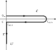
Refer to caption
Figure 1: Closed real-time path 𝒞\mathcalbf{C}. This time path was invented by Schwinger [11] and applied to non-equilibrium problems by Keldysh [14] (see also Refs. [12, 13]). In order to avoid the doubling of the degrees of freedom, we use the form presented in Ref. [15].

This work is organized as follows: In section II, we derive Kadanoff-Baym equations for non-Gaussian initial states from the corresponding 2PI effective action using the explicit technique. In section III, we provide techniques for calculating the non-Gaussian initial correlations αn𝑡ℎ​(x1,…,xn)\alpha_{n}^{\it th}(x_{1},\dots,x_{n}) within perturbation theory. These techniques are generalized to the nonperturbative 2PI case in section IV. In section V, Kadanoff-Baym equations for a thermal initial state are derived by combining the results from sections II and IV. In section VI, we compare numerical solutions of Kadanoff-Baym equations for two nonequilibrium initial states that are approximations to the thermal initial state. One of them is Gaussian, while the other also includes the leading non-Gaussian initial correlation. The appendices A and B contain additional material helpful for sections III and IV, respectively.

II Effective Action and Kadanoff-Baym equations

II.1 Gaussian Initial States

In this subsection, we start from the classical action for a real scalar quantum field with a quartic self interaction

S⁡[ϕ]=∫d4​x​(12​(∂ϕ)2−12​m2​ϕ2−λ4!​ϕ4),S[\phi]=\int d^{4}x\,\left(\frac{1}{2}(\partial\phi)^{2}-\frac{1}{2}m^{2}\phi^{2}-\frac{\lambda}{4!}\phi^{4}\right)\;, (1)

and review the basic elements of the derivation of the 2PI effective action and the Kadanoff-Baym equations for the case of a Gaussian initial state. In the following subsections, we can then easily expose the differences, which arise for a non-Gaussian initial state.

The Schwinger-Keldysh propagator is defined by

G⁡(x,y)=⟨T​C​Φ​(x)​Φ​(y)⟩−⟨Φ⁡(x)⟩​⟨Φ⁡(y)⟩,G(x,y)=\left\langle T{C}\,\Phi(x)\Phi(y)\right\rangle-\left\langle\Phi(x)\right\rangle\left\langle\Phi(y)\right\rangle\;, (2)

where T​CT{C} denotes the time-ordering operator along the closed real-time path 𝒞\mathcalbf{C} shown in figure 1 [11, 14, 15]. The Schwinger-Keldysh propagator can be obtained by functional differentiation from the generating functional for correlation functions formulated on the closed real-time path. The generating functional in the presence of a local external source J⁡(x)J(x) and a bilocal external source K⁡(x,y)K(x,y) is given by [44]

Zρ​[J,K]=∫𝒟​φ​(x)​⟨φ+​|ρ|​φ−⟩\displaystyle Z_{\rho}\left[J,K\right]=\int\mathcal{D}\varphi\left(x\right)\left\langle\varphi_{+}\left|\rho\right|\varphi_{-}\right\rangle (3)
×exp⁡(i​S​[φ]+i​J​φ+i2​φ​K​φ),\displaystyle{}\times\exp\left(iS\left[\varphi\right]+iJ\varphi+\frac{i}{2}\varphi K\varphi\right)\;,

where a matrix-vector notation has been used for the space-time integrals in the exponential function11 1 Throughout this work, the compact notation of Ref. [15] is used for the contour integrals over the closed real-time path, for example J​φ≡∫C​d4​x​J​(x)​φ​(x)=∫d4​x​[J+​(x)​φ+​(x)−J−​(x)​φ−​(x)]J\varphi\equiv\int{C}\!d^{4}x\,J(x)\varphi(x)=\int\!d^{4}x\left[J_{+}(x)\varphi_{+}(x)-J_{-}(x)\varphi_{-}(x)\right]. , and |φ±⟩|\varphi_{\pm}\rangle are the quantum states corresponding to the field configurations φ±​(𝒙)=φ⁡(0±,𝒙)\varphi_{\pm}(\bm{x})=\varphi(0_{\pm},\bm{x}). The information about the initial state enters via the matrix element of the density matrix ρ\rho, which is known only at the initial time t=ti​n​i​t≡0t=t_{init}\equiv 0.

A Gaussian initial state is an initial state for which all connected nn-point correlation functions with n≥3n\geq 3 vanish at the initial time. The density matrix element for a Gaussian initial state can be parameterized by

⟨φ+​|ρ|​φ−⟩=exp⁡(i​α0+i​α1​φ+i2​φ​α2​φ).\left\langle\varphi_{+}\left|\rho\right|\varphi_{-}\right\rangle=\exp\left(i\alpha_{0}+i\alpha_{1}\varphi+\frac{i}{2}\varphi\alpha_{2}\varphi\right)\;. (4)

Therefore, in the Gaussian case, the contribution of the density matrix to the generating functional (3) can formally be absorbed into the external sources, J+α1→JJ+\alpha_{1}\rightarrow J and K+α2→KK+\alpha_{2}\rightarrow K. As is, for example, explained in Ref. [48], this means that the Gaussian initial density matrix does not appear explicitly, but rather enters the dynamics via defining the initial conditions of all independent one- and two-point functions. For vanishing field expectation value, these are given by G⁡(x,y)G(x,y), (∂x0+∂y0)G(x,y)(\partial_{x^{0}}+\partial_{y^{0}})G(x,y) and ∂x0∂y0G⁡(x,y)\partial_{x^{0}}\partial_{y^{0}}G(x,y), all evaluated at x0=y0=0x^{0}=y^{0}=0 [48, 9].

The 2PI effective action Γ⁡[ϕ,G]\Gamma[\phi,G] is the double Legendre transform of the generating functional (3) with respect to the external sources. For a Gaussian initial state, the generating functional has the same structure as the generating functional in vacuum, except that all time-integrations are performed over the closed real-time path. Consequently, for a Gaussian initial state the 2PI effective action can be parameterized in the form [10]

Γ⁡[ϕ,G]\displaystyle\Gamma\left[\phi,G\right] =\displaystyle= S⁡[ϕ]+i2​Tr​log𝒞​[G−1]\displaystyle S\left[\phi\right]+\frac{i}{2}\mbox{Tr}\log_{\mathcalbf{C}}\left[G^{-1}\right] (5)
+i2​Tr𝒞​[𝒢0−1​G]+Γ2​[ϕ,G],\displaystyle{}+\frac{i}{2}\mbox{Tr}_{\mathcalbf{C}}\left[\mathcal{G}_{0}^{-1}G\right]+\Gamma_{2}\left[\phi,G\right]\;,

where 𝒢0−1{\mathcal{G}_{0}}^{-1} is the inverse classical Schwinger-Keldysh propagator and i​Γ2​[ϕ,G]i\Gamma_{2}[\phi,G] is the sum of all 2PI Feynman diagrams without any external legs, where internal lines represent the complete Schwinger-Keldysh propagator G⁡(x,y)G(x,y). The vertices of the diagrams contained in i​Γ2​[ϕ,G]i\Gamma_{2}[\phi,G] are given by the third and fourth functional derivatives of the classical action S⁡[ϕ]S[\phi] [10]. Eventually, the Kadanoff-Baym equations

(□x+M2​(x))​GF​(x,y)\displaystyle\left(\Box_{x}+M^{2}(x)\right)G_{F}(x,y) =\displaystyle= ∫0y0d4​z​ΠF​(x,z)​Gρ​(z,y)\displaystyle\int\limits_{0}^{y^{0}}d^{4}z\;\Pi_{F}(x,z)G_{\rho}(z,y) (6)
−∫0x0d4zΠρ(x,z)GF(z,y),\displaystyle\hskip-42.67912pt{}-\int\limits_{0}^{x^{0}}d^{4}z\;\Pi_{\rho}(x,z)G_{F}(z,y)\;,
(□x+M2​(x))​Gρ​(x,y)\displaystyle\left(\Box_{x}+M^{2}(x)\right)G_{\rho}(x,y) =\displaystyle= ∫x0y0d4​z​Πρ​(x,z)​Gρ​(z,y),\displaystyle\int\limits_{x^{0}}^{y^{0}}d^{4}z\;\Pi_{\rho}(x,z)G_{\rho}(z,y)\;,

follow from the stationarity condition of the 2PI effective action. Here, we use the notation of Ref. [9].

II.2 Non-Gaussian Initial States

In the remainder of this section, Kadanoff-Baym equations are derived that can describe systems characterized by a general non-Gaussian initial state [44, 43, 49]. For that purpose, we extend the derivation of the previous subsection using a generalization of the Gaussian density matrix (4). In general, the matrix element of the density matrix ρ\rho is an arbitrary functional of the field configurations φ+​(𝒙)\varphi_{+}(\bm{x}) and φ−​(𝒙)\varphi_{-}(\bm{x}), which can be written as [44]

⟨φ+​|ρ|​φ−⟩=exp⁡(i​F​[φ]).\left\langle\varphi_{+}\left|\rho\right|\varphi_{-}\right\rangle=\exp\left(iF[\varphi]\right)\;. (7)

While for a Gaussian initial state F⁡[φ]F[\varphi] is a quadratic functional of the field, for a general non-Gaussian initial state it may be Taylor expanded in the form [44]

F⁡[φ]\displaystyle F[\varphi] =\displaystyle= ∑n=0∞1n!​∫𝒞d4​x1​…​d4​xn​αn​(x1,…,xn)\displaystyle\sum_{n=0}^{\infty}\frac{1}{n!}\int\limits_{\mathcalbf{C}}d^{4}x_{1}\ldots d^{4}x_{n}\;\alpha_{n}\left(x_{1},\ldots,x_{n}\right) (8)
×φ⁡(x1)⋅…⋅φ⁡(xn).\displaystyle{}\times\varphi(x_{1})\cdot\ldots\cdot\varphi(x_{n})\;.

By definition F⁡[φ]F[\varphi] depends only on the field configuration evaluated at the boundaries of the time contour. Consequently, the kernels αn​(x1,…,xn)\alpha_{n}(x_{1},\dots,x_{n}) are non-zero only if all their time arguments lie on the boundaries of the time contour. With the notation δ+​(t)=δ​C​(t−0+)\delta_{+}(t)=\delta{C}(t-0_{+}) and δ−​(t)=δ​C​(t−0−)\delta_{-}(t)=\delta{C}(t-0_{-}), they can be written in the form

αn​(x1,…,xn)\displaystyle\alpha_{n}\left(x_{1},\ldots,x_{n}\right) =\displaystyle= αnϵ1,…,ϵn​(𝒙𝟏,…,𝒙𝒏)\displaystyle\alpha_{n}^{\epsilon_{1},\ldots,\epsilon_{n}}\left(\bm{x_{1}},\ldots,\bm{x_{n}}\right) (9)
×δϵ1​(x10)⋅…⋅δϵn​(xn0),\displaystyle{}\times\delta_{\epsilon_{1}}\left(x_{1}^{0}\right)\cdot\ldots\cdot\delta_{\epsilon_{n}}\left(x_{n}^{0}\right)\;,

where summation over ϵj∈{+,−}\epsilon_{j}\in\{+,-\} is implied. In this way, the explicit dependence of the functional F⁡[φ]F[\varphi] on the field configurations φ+​(𝒙)\varphi_{+}(\bm{x}) and φ−​(𝒙)\varphi_{-}(\bm{x}) may be recovered,

F⁡[φ]=α0+∫d3​x​α1ϵ​(𝒙)​φϵ​(𝒙)+….F[\varphi]=\alpha_{0}+\int d^{3}x\;\alpha_{1}^{\epsilon}(\bm{x})\varphi_{\epsilon}(\bm{x})+\ldots\;.

The set of all kernels αn\alpha_{n} with n≥0n\geq 0 encodes the complete information about the density matrix characterizing the initial state. Not all the kernels are independent. The Hermiticity of the density matrix, ρ=ρ†\rho=\rho^{\dagger}, implies that

i​αnϵ1,…,ϵn​(𝒙𝟏,…,𝒙𝒏)=(i​αn(−ϵ1),…,(−ϵn)​(𝒙𝟏,…,𝒙𝒏))∗.i\alpha_{n}^{\epsilon_{1},\dots,\epsilon_{n}}(\bm{x_{1}},\dots,\bm{x_{n}})=\left(i\alpha_{n}^{(-\epsilon_{1}),\dots,(-\epsilon_{n})}(\bm{x_{1}},\dots,\bm{x_{n}})\right)^{*}\;.

If the initial state is invariant under some symmetries, there are further constraints. For example, for an initial state which is invariant under the Z2Z_{2}-symmetry Φ→−Φ\Phi\rightarrow-\Phi, all kernels αn​(x1,…,xn)\alpha_{n}(x_{1},\dots,x_{n}) with odd nn vanish. If the initial state is homogeneous in space, the initial correlations αn​(x1,…,xn)\alpha_{n}(x_{1},\dots,x_{n}) are invariant under space-translations 𝒙𝒊→𝒙𝒊+𝒂\bm{x_{i}}\rightarrow\bm{x_{i}}+\bm{a} of all arguments for any real three-vector 𝒂\bm{a}, and can conveniently be expressed in spatial momentum space,

αnϵ1,…,ϵn​(𝒙𝟏,…,𝒙𝒏)\displaystyle\alpha_{n}^{\epsilon_{1},\ldots,\epsilon_{n}}(\bm{x_{1}},\ldots,\bm{x_{n}})
=\displaystyle= ∫d3​k1(2​π)3​…​∫d3​kn(2​π)3​exp⁡(i​∑j𝒌𝒋​𝒙𝒋)\displaystyle\int\frac{d^{3}k_{1}}{(2\pi)^{3}}\ldots\int\frac{d^{3}k_{n}}{(2\pi)^{3}}\;\exp\left(i\sum_{j}\bm{k_{j}x_{j}}\right)
×(2​π)3​δ3​(𝒌𝟏+⋯+𝒌𝒏)​αnϵ1,…,ϵn​(𝒌𝟏,…,𝒌𝒏).\displaystyle{}\times(2\pi)^{3}\delta^{3}(\bm{k_{1}}+\dots+\bm{k_{n}})\alpha_{n}^{\epsilon_{1},\dots,\epsilon_{n}}(\bm{k_{1}},\dots,\bm{k_{n}})\;.

Summarizing, the generating functional reads

Zρ​[J,K]\displaystyle Z_{\rho}[J,K] =\displaystyle= ∫𝒟​φ​exp⁡(i​S​[φ]CLOSE\displaystyle\int\mathcal{D}\varphi\;\exp\Big(iS[\varphi] (10)
OPEN+i​J​φ+i2​φ​K​φ+i​F3​[φ]),\displaystyle{}+iJ\varphi+\frac{i}{2}\,\varphi K\varphi+iF_{3}[\varphi]\Big)\;,

where the kernels α0\alpha_{0}, α1\alpha_{1} and α2\alpha_{2} have been absorbed into the measure 𝒟​φ\mathcal{D}{\varphi} and into the sources JJ and KK, respectively. The functional F3​[φ]≡F3​[φ;α3,α4,…]F_{3}[\varphi]\equiv F_{3}[\varphi;\alpha_{3},\alpha_{4},\dots] contains the contributions of third, fourth and higher orders of the Taylor expansion (8) and vanishes for a Gaussian initial state.

II.3 2PI Effective Action for Non-Gaussian Initial States

According to eq. (10), the 2PI effective action in the presence of non-Gaussian correlations is obtained from the standard parameterization [10] of the 2PI effective action applied to a theory described by the modified classical action S~​[ϕ]≡S⁡[ϕ]+F3​[ϕ],\tilde{S}[\phi]\equiv S[\phi]+F_{3}[\phi],

Γ⁡[ϕ,G]\displaystyle\Gamma\left[\phi,G\right] =\displaystyle= S~​[ϕ]+i2​Tr​log𝒞​[G−1]\displaystyle\tilde{S}\left[\phi\right]+\frac{i}{2}\mbox{Tr}\log_{\mathcalbf{C}}\left[G^{-1}\right] (11)
+i2​Tr𝒞​[𝒢~0−1​G]+Γ~2​[ϕ,G]\displaystyle{}+\frac{i}{2}\mbox{Tr}_{\mathcalbf{C}}\left[\tilde{\mathcal{G}}_{0}^{-1}G\right]+\tilde{\Gamma}_{2}\left[\phi,G\right]
≡\displaystyle\equiv ΓG​[ϕ,G]+Γn​G​[ϕ,G],\displaystyle\Gamma_{G}[\phi,G]+\Gamma_{nG}[\phi,G]\;,

where i​𝒢~0−1​(x,y)≡δ2​S~​[ϕ]/δ​ϕ​(x)​δ​ϕ​(y)i\tilde{\mathcal{G}}_{0}^{-1}(x,y)\equiv\delta^{2}\tilde{S}[\phi]/\delta\phi(x)\delta\phi(y). The Gaussian part ΓG​[ϕ,G]\Gamma_{G}[\phi,G] coincides with the right-hand side of eq. (5), and the non-Gaussian part is given by

Γn​G​[ϕ,G]=F3​[ϕ]+12​Tr​C​[δ2​F3δ​ϕ​δ​ϕ​G]+Γ2,n​G​[ϕ,G],\Gamma_{nG}[\phi,G]=F_{3}[\phi]+\frac{1}{2}\mbox{Tr}{C}\left[\frac{\delta^{2}F_{3}}{\delta\phi\delta\phi}G\right]+\Gamma_{2,\,nG}[\phi,G]\,,

where

Γ2,n​G​[ϕ,G]≡Γ~2​[ϕ,G]−Γ2​[ϕ,G].\Gamma_{2,\,nG}[\phi,G]\equiv\tilde{\Gamma}_{2}[\phi,G]-\Gamma_{2}[\phi,G]\;.

The modified 2PI functional i​Γ~2​[ϕ,G]i\tilde{\Gamma}_{2}[\phi,G] is equal to the sum of all 2PI Feynman diagrams without any external legs, where internal lines represent the complete propagator G⁡(x,y)G(x,y) and where vertices are given by the functional derivatives of the modified classical action S~​[ϕ]=S⁡[ϕ]+F3​[ϕ]\tilde{S}[\phi]=S[\phi]+F_{3}[\phi]. The contribution from the classical action S⁡[ϕ]S[\phi] leads to the classical local three- and four-point vertices. Additionally, the contribution from the functional F3​[ϕ]F_{3}[\phi] leads to effective non-local vertices, which contain the non-Gaussian initial nn-point correlations with n≥3n\geq 3 (see figure 2),

i​δn​F3​[ϕ]δ​ϕ​(x1)​…​δ​ϕ​(xn)≡i​α¯n​(x1,…,xn).i\frac{\delta^{n}F_{3}[\phi]}{\delta\phi(x_{1})\dots\delta\phi(x_{n})}\equiv i\bar{\alpha}_{n}(x_{1},\dots,x_{n}). (12)

These effective nn-point vertices are only supported at the initial time, and can be parameterized analogously to eq. (9). For a Z2Z_{2}-symmetric initial state, the field expectation value vanishes, ϕ⁡(x)=0\phi(x)=0, such that α¯n​(x1,…,xn)=αn​(x1,…,xn)\bar{\alpha}_{n}(x_{1},\dots,x_{n})=\alpha_{n}(x_{1},\dots,x_{n}).

Refer to caption

Figure 2: Non-local effective vertices i​α¯n​(x1,…,xn)i\bar{\alpha}_{n}(x_{1},\dots,x_{n}) connecting nn lines for n=3,4,5,6n=3,4,5,6 encoding the non-Gaussian three-, four-, five-, and six-point correlations of the initial state.

The contribution of these effective non-local vertices is most important close to the initial time. For example, a non-zero four-point source α4​(x1,…,x4)\alpha_{4}(x_{1},\dots,x_{4}) leads to a non-vanishing value of the connected four-point correlation function at the initial time, which is impossible for a Gaussian initial state.

Note that those 2PI diagrams that contain exclusively the classical vertices contribute to the functional i​Γ2​[ϕ,G]i\Gamma_{2}[\phi,G] by definition. Therefore, the diagrams contributing to the non-Gaussian part i​Γ2,n​G​[ϕ,G]i\Gamma_{2,\,nG}[\phi,G] contain at least one effective vertex from eq. (12).

In section VI we study the numerical solution of Kadanoff-Baym equations for a Z2Z_{2}-symmetric non-Gaussian initial state with a non-zero initial 4-point correlation. In this case the 2PI functional Γ~2\tilde{\Gamma}_{2} reads in ‘‘naïve’’22 2 This means that non-local effective vertices do not affect the counting of loops. three-loop approximation (see figure 3)

i​Γ~2​[G]=18​∫𝒞d4​x1234​[−i​λ​δ12​δ23​δ34+i​α1234]​G12​G34\displaystyle i\tilde{\Gamma}_{2}[G]=\frac{1}{8}\int\limits_{\mathcalbf{C}}d^{4}x_{1234}\left[\rule{0.0pt}{11.38109pt}-i\lambda\delta_{12}\delta_{23}\delta_{34}+i\alpha_{1234}\right]G_{12}G_{34} (13)
+148∫𝒞d4x1⋯8[−iλδ12δ23δ34+iα1234]\displaystyle{}+\frac{1}{48}\int\limits_{\mathcalbf{C}}d^{4}x_{1\cdots 8}\left[\rule{0.0pt}{11.38109pt}-i\lambda\delta_{12}\delta_{23}\delta_{34}+i\alpha_{1234}\right]
×G15​G26​G37​G48​[−i​λ​δ56​δ57​δ58+i​α5678],\displaystyle{}\times\,G_{15}G_{26}G_{37}G_{48}\left[\rule{0.0pt}{11.38109pt}-i\lambda\delta_{56}\delta_{57}\delta_{58}+i\alpha_{5678}\right]\;,\hskip 28.45274pt

where G12=G⁡(x1,x2)G_{12}=G(x_{1},x_{2}) and α1234=α4​(x1,x2,x3,x4)\alpha_{1234}=\alpha_{4}(x_{1},x_{2},x_{3},x_{4}). Note that the contribution to the mixed basketball diagram in the second and third line with one classical and one effective vertex appears twice, which accounts for the symmetry factor 1/241/24.

Refer to caption

Figure 3: Diagrams contributing to the three-loop truncation of the 2PI effective action in the symmetric phase (setting-sun approximation) in the presence of an effective non-local four-point vertex.

II.4 Self-Energy for Non-Gaussian Initial States

The equation of motion for the complete propagator obtained from eq. (11) reads

G−1​(x,y)=𝒢0−1​(x,y)−Π⁡(x,y)−i​α¯2​(x,y),G^{-1}(x,y)=\mathcal{G}_{0}^{-1}(x,y)-\Pi(x,y)-i\bar{\alpha}_{2}(x,y)\,, (14)

where α¯2=α2+δ2​F3​[ϕ]/δ​ϕ​δ​ϕ\bar{\alpha}_{2}=\alpha_{2}+\delta^{2}F_{3}[\phi]/\delta\phi\delta\phi and the complete self-energy is given by

Π⁡(x,y)\displaystyle\Pi(x,y) =\displaystyle= 2​i​δ​Γ~2​[ϕ,G]δ​G​(y,x)\displaystyle\frac{2i\delta\tilde{\Gamma}_{2}[\phi,G]}{\delta G(y,x)} (15)
=\displaystyle= 2​i​δ​Γ2​[ϕ,G]δ​G​(y,x)+2​i​δ​Γ2,n​G​[ϕ,G]δ​G​(y,x)\displaystyle\frac{2i\delta\Gamma_{2}[\phi,G]}{\delta G(y,x)}+\frac{2i\delta\Gamma_{2,\,nG}[\phi,G]}{\delta G(y,x)}
≡\displaystyle\equiv ΠG​(x,y)+Πn​G​(x,y),\displaystyle\Pi^{G}(x,y)+\Pi^{nG}(x,y)\,,

where ΠG\Pi^{G} contains the contributions to the self energy, which are also present for a Gaussian initial state, and the non-Gaussian part Πn​G\Pi^{nG} contains diagrams with at least one non-local effective vertex. They can be further decomposed as

ΠG​(x,y)\displaystyle\Pi^{\it G}(x,y) =\displaystyle= −i​Π𝑙𝑜𝑐​(x)​δ​C​(x−y)+Π𝑛𝑜𝑛−𝑙𝑜𝑐G​(x,y),\displaystyle-i\Pi_{\it loc}(x)\delta{C}(x-y)+\Pi^{\it G}_{\it non-loc}(x,y)\,,
Π𝑛𝐺​(x,y)\displaystyle\Pi^{\it nG}(x,y) =\displaystyle= i​Π𝑠𝑢𝑟𝑓𝑎𝑐𝑒𝑛𝐺​(x,y)+Π𝑛𝑜𝑛−𝑙𝑜𝑐𝑛𝐺​(x,y).\displaystyle i\Pi^{\it nG}_{\it surface}(x,y)+\Pi^{\it nG}_{\it non-loc}(x,y)\,. (16)

The non-Gaussian non-local part Π𝑛𝑜𝑛−𝑙𝑜𝑐𝑛𝐺​(x,y)\Pi^{\it nG}_{\it non-loc}(x,y) contains diagrams where both external lines are attached to a standard vertex. The non-Gaussian “surface” part i​Π𝑠𝑢𝑟𝑓𝑎𝑐𝑒𝑛𝐺​(x,y)i\Pi^{\it nG}_{\it surface}(x,y) contains diagrams where at least one external line is attached to a non-local effective vertex. Thus, the surface part is supported only at the initial time surface where x0=0x^{0}=0 or y0=0y^{0}=0. In general, such contributions can arise in the following ways:

  1. 1.

    From diagrams where both external lines are connected to an effective non-local vertex as given in eq. (12). They are supported at x0=y0=0x^{0}=y^{0}=0.

  2. 2.

    From diagrams where one of the two external lines is connected to an effective non-local vertex, while the other one is connected to a classical local vertex. They are supported at x0=0,y0≥0x^{0}=0,y^{0}\geq 0 or vice-versa.

  3. 3.

    Via the contribution i​α¯2​(x,y)i\bar{\alpha}_{2}(x,y) of the initial two-point source which is supported at x0=y0=0x^{0}=y^{0}=0. This is the only Gaussian surface-contribution.

Refer to caption

Figure 4: Diagrams contributing to the self-energy Π⁡(x,y)\Pi(x,y) in setting-sun approximation in the presence of an effective non-local four-point vertex. From left to right, the diagrams contribute to Π𝑙𝑜𝑐\Pi_{\it loc}, Π𝑛𝑜𝑛−𝑙𝑜𝑐G\Pi^{G}_{\it non-loc}, Πλ​α\Pi_{\lambda\alpha}, Πα​λ\Pi_{\alpha\lambda}, and the last two both contribute to Πα​α\Pi_{\alpha\alpha}.

Accordingly, the contributions to the self-energy which are supported at the initial time surface can be further decomposed as

Π𝑠𝑢𝑟𝑓𝑎𝑐𝑒​(x,y)\displaystyle\Pi_{\it surface}(x,y) =\displaystyle= Π𝑠𝑢𝑟𝑓𝑎𝑐𝑒𝑛𝐺​(x,y)+α¯2​(x,y)\displaystyle\Pi^{\it nG}_{\it surface}(x,y)+\bar{\alpha}_{2}(x,y)
≡\displaystyle\equiv Πα​α​(x,y)+Πλ​α​(x,y)+Πα​λ​(x,y),\displaystyle\Pi_{\alpha\alpha}(x,y)+\Pi_{\lambda\alpha}(x,y)+\Pi_{\alpha\lambda}(x,y),

where

Πα​α​(x,y)\displaystyle\Pi_{\alpha\alpha}(x,y) =\displaystyle= δϵ1​(x0)​Πα​αϵ1,ϵ2​(𝒙,𝒚)​δϵ2​(y0),\displaystyle\delta_{\epsilon_{1}}(x^{0})\Pi_{\alpha\alpha}^{\epsilon_{1},\epsilon_{2}}(\bm{x},\bm{y})\delta_{\epsilon_{2}}(y^{0})\,,
Πλ​α​(x,y)\displaystyle\Pi_{\lambda\alpha}(x,y) =\displaystyle= Πλ​αϵ​(x0,𝒙,𝒚)​δϵ​(y0),\displaystyle\Pi_{\lambda\alpha}^{\epsilon}(x^{0},\bm{x},\bm{y})\delta_{\epsilon}(y^{0})\,, (17)
Πα​λ​(x,y)\displaystyle\Pi_{\alpha\lambda}(x,y) =\displaystyle= δϵ​(x0)​Πα​λϵ​(𝒙,y0,𝒚)=Πλ​α​(y,x).\displaystyle\delta_{\epsilon}(x^{0})\Pi_{\alpha\lambda}^{\epsilon}(\bm{x},y^{0},\bm{y})\ =\ \Pi_{\lambda\alpha}(y,x)\,.

Πα​α\Pi_{\alpha\alpha} contains all contributions of type (1.) and (3.). Diagrams of type (2.) contribute to Πλ​α\Pi_{\lambda\alpha} or Πα​λ\Pi_{\alpha\lambda} depending which external line is attached to the effective non-local vertex and which to the classical local vertex. For all diagrams contributing to Πλ​α\Pi_{\lambda\alpha} the left line is connected to the classical four- or three-point vertex. The non-local part of the self-energy can be split into statistical and spectral components, similarly to the Gaussian case,

Π𝑛𝑜𝑛−𝑙𝑜𝑐​(x,y)\displaystyle\Pi_{\it non-loc}(x,y) ≡\displaystyle\equiv Π𝑛𝑜𝑛−𝑙𝑜𝑐G​(x,y)+Π𝑛𝑜𝑛−𝑙𝑜𝑐𝑛𝐺​(x,y)\displaystyle\Pi^{\it G}_{\it non-loc}(x,y)+\Pi^{\it nG}_{\it non-loc}(x,y) (18)
≡\displaystyle\equiv ΠF​(x,y)−i2​sign​C​(x0−y0)​Πρ​(x,y).\displaystyle\Pi_{F}(x,y)-\frac{i}{2}\,\mbox{sign}{C}(x^{0}-y^{0})\,\Pi_{\rho}(x,y)\,.

The local part of the self-energy is identical to the Gaussian case and is included in the effective time-dependent mass term M2​(x)=m2+Πl​o​c​(x)M^{2}(x)=m^{2}+\Pi_{loc}(x).

For the setting-sun approximation from eq. (13), the self-energy is given by (see figure 4)

Πn​o​n−l​o​cG​(x,y)\displaystyle\Pi^{G}_{non-loc}(x,y) =\displaystyle= (−i​λ)26​G​(x,y)3,\displaystyle\frac{(-i\lambda)^{2}}{6}G(x,y)^{3}\,,
Πn​o​n−l​o​cn​G​(x,y)\displaystyle\Pi^{nG}_{non-loc}(x,y) =\displaystyle= 0,\displaystyle 0\,,
i​Πα​α​(x,y)\displaystyle i\Pi_{\alpha\alpha}(x,y) =\displaystyle= i​α2​(x,y)+12​∫d4​x34​i​αx​y​34​G34\displaystyle i\alpha_{2}(x,y)+\frac{1}{2}\int\!\!d^{4}\!x_{34}\,i\alpha_{xy34}G_{34}
+16∫d4x2⋯7iαx​234G25G36G47iα567​y,\displaystyle{}+\frac{1}{6}\int\!\!d^{4}\!x_{2\cdots 7}\,i\alpha_{x234}G_{25}G_{36}G_{47}\,i\alpha_{567y}\,,
i​Πλ​α​(x,y)\displaystyle i\Pi_{\lambda\alpha}(x,y) =\displaystyle= −i​λ6​∫d4​x123​Gx​1​Gx​2​Gx​3​i​α123​y,\displaystyle\frac{-i\lambda}{6}\int\!\!d^{4}\!x_{123}\,G_{x1}G_{x2}G_{x3}\,i\alpha_{123y}\,,
i​Πα​λ​(x,y)\displaystyle i\Pi_{\alpha\lambda}(x,y) =\displaystyle= −i​λ6​∫d4​x234​i​αx​234​G2​y​G3​y​G4​y.\displaystyle\frac{-i\lambda}{6}\int\!\!d^{4}\!x_{234}\,i\alpha_{x234}\,G_{2y}G_{3y}G_{4y}\,.

II.5 Kadanoff-Baym Equations for Non-Gaussian Initial States

Convoluting eq. (14) with the complete propagator yields

(□x+M2​(x))​G​(x,y)=−i​δ𝒞​(x−y)\displaystyle\left(\Box_{x}+M^{2}(x)\right)G(x,y)=-i\delta_{\mathcalbf{C}}(x-y) (19)
−i∫𝒞d4z[Πn​o​n−l​o​c(x,z)+iΠλ​α(x,z)]G(z,y).\displaystyle{}-i\int\limits_{\mathcalbf{C}}d^{4}z\;\left[\Pi_{non-loc}(x,z)+i\Pi_{\lambda\alpha}(x,z)\right]G(z,y)\;.

The second line follows from the parameterization (16) of the self-energy, and assuming x0>0x^{0}>0 and y0>0y^{0}>0. Using eqs. (17,18) and transforming to spatial momentum space yields the Kadanoff-Baym equations for GF​(x0,y0,𝒌)G_{F}(x^{0},y^{0},\bm{k}) and Gρ​(x0,y0,𝒌)G_{\rho}(x^{0},y^{0},\bm{k}) for spatially homogeneous non-Gaussian initial states,

(∂x02+𝒌2+M2(x0))GF(x0,y0,𝒌)\displaystyle\left(\partial_{x^{0}}^{2}+\bm{k}^{2}+M^{2}(x^{0})\right)G_{F}(x^{0},y^{0},\bm{k}) =\displaystyle= ∫0y0d​z0​ΠF​(x0,z0,𝒌)​Gρ​(z0,y0,𝒌)−∫0x0d​z0​Πρ​(x0,z0,𝒌)​GF​(z0,y0,𝒌)\displaystyle\int\limits_{0}^{y^{0}}\!\!dz^{0}\,\Pi_{F}(x^{0},z^{0},\bm{k})G_{\rho}(z^{0},y^{0},\bm{k})-\int\limits_{0}^{x^{0}}\!\!dz^{0}\,\Pi_{\rho}(x^{0},z^{0},\bm{k})G_{F}(z^{0},y^{0},\bm{k}) (20)
+Πλ​α,F​(x0,𝒌)​GF​(0,y0,𝒌)+14​Πλ​α,ρ​(x0,𝒌)​Gρ​(0,y0,𝒌),\displaystyle{}+\Pi_{\lambda\alpha,F}(x^{0},\bm{k})G_{F}(0,y^{0},\bm{k})+\frac{1}{4}\Pi_{\lambda\alpha,\rho}(x^{0},\bm{k})G_{\rho}(0,y^{0},\bm{k})\;,

and

(∂x02+𝒌2+M2(x0))Gρ(x0,y0,𝒌)\displaystyle\left(\partial_{x^{0}}^{2}+\bm{k}^{2}+M^{2}(x^{0})\right)G_{\rho}(x^{0},y^{0},\bm{k}) =\displaystyle= ∫x0y0d​z0​Πρ​(x0,z0,𝒌)​Gρ​(z0,y0,𝒌),\displaystyle\int\limits_{x_{0}}^{y^{0}}\!\!dz^{0}\,\Pi_{\rho}(x^{0},z^{0},\bm{k})G_{\rho}(z^{0},y^{0},\bm{k})\,,

where

Πλ​α,F​(x0,𝒌)\displaystyle\Pi_{\lambda\alpha,F}(x^{0},\bm{k}) =\displaystyle= Πλ​α+​(x0,𝒌)+Πλ​α−​(x0,𝒌),\displaystyle\Pi_{\lambda\alpha}^{+}(x^{0},\bm{k})+\Pi_{\lambda\alpha}^{-}(x^{0},\bm{k})\,,
Πλ​α,ρ​(x0,𝒌)\displaystyle\Pi_{\lambda\alpha,\rho}(x^{0},\bm{k}) =\displaystyle= 2​i​(Πλ​α+​(x0,𝒌)−Πλ​α−​(x0,𝒌)).\displaystyle 2i\left(\Pi_{\lambda\alpha}^{+}(x^{0},\bm{k})-\Pi_{\lambda\alpha}^{-}(x^{0},\bm{k})\right)\,.

Thus, for a non-Gaussian initial state, the right-hand side of the Kadanoff-Baym equation for the statistical propagator is modified. In addition to the memory integrals there are now new contributions originating from the non-Gaussian initial correlations. Unlike the memory integrals, these new contributions do not have to vanish in the limit x0,y0→0x^{0},y^{0}\rightarrow 0. This is due to the fact that the higher non-Gaussian correlations of the initial state can lead to a non-vanishing value of the connected four- and three-point correlation functions at the initial time.

III Thermal Initial Correlations: Perturbation Theory
Refer to caption
Figure 5: The thermal time contour 𝒞+ℐ\mathcalbf{C}\!+\!\mathcalbf{I} is obtained by concatenating the closed real-time contour 𝒞\mathcalbf{C} and the imaginary time contour ℐ\mathcalbf{I} running from t=0t=0 to t=−i​βt=-i\beta [40, 41, 42, 45, 46]. We employ this time path in order to infer the initial correlation functions αn𝑡ℎ​(x1,…,xn)\alpha_{n}^{\it th}(x_{1},\dots,x_{n}) required for describing thermal equilibrium on the Schwinger-Keldysh closed real-time path 𝒞\mathcalbf{C} with finite initial time shown in figure 1.

In order to derive Kadanoff-Baym equations that are capable of describing thermal equilibrium, the thermal density matrix

ρt​h=1Z​exp⁡(−β​H),\rho_{th}=\frac{1}{Z}\,\exp\left(-\beta H\right)\,,

has to be represented by a Taylor expansion in terms of thermal correlation functions αn𝑡ℎ​(x1,…,xn)\alpha_{n}^{\it th}(x_{1},\dots,x_{n}) as in eqs. (7, 8). These thermal correlation functions do then enter the Kadanoff-Baym equations in the form of non-local effective vertices, as described in the previous section.

The thermal correlations functions αn𝑡ℎ​(x1,…,xn)\alpha_{n}^{\it th}(x_{1},\dots,x_{n}) can be calculated order-by-order in the coupling constant within usual perturbation theory (see appendix A). However, in the context of Kadanoff-Baym equations, it is necessary to use approximations of the thermal correlation functions that are compatible with the underlying truncation of the 2PI effective action. It is a major purpose of this paper to provide computational techniques for identifying suitable approximations of the thermal correlation functions αn𝑡ℎ​(x1,…,xn)\alpha_{n}^{\it th}(x_{1},\dots,x_{n}).

For simplicity, in this section, we first present the computational techniques within perturbation theory. In the following section, these techniques are then generalized to the nonperturbative 2PI formalism.

The main idea is to determine the functions αn𝑡ℎ​(x1,…,xn)\alpha_{n}^{\it th}(x_{1},\dots,x_{n}) by matching the description of thermal equilibrium based on the closed real-time path 𝒞\mathcalbf{C} in the presence of effective vertices αn𝑡ℎ\alpha_{n}^{\it th} (“ 𝒞+α\mathcalbf{C}\!+\!\alpha ”) on the one hand with the well-known equivalent description based on the thermal time path (“ 𝒞+ℐ\mathcalbf{C}\!+\!\mathcalbf{I} ”) [40, 41, 42, 45, 46] shown in figure 5 on the other hand.

The generating functional for these two descriptions is obtained by inserting the respective representations of the thermal density matrix,

⟨φ+​|ρt​h|​φ−⟩={∫φ⁡(0,𝒙)=φ−​(𝒙)φ⁡(−i​β,𝒙)=φ+​(𝒙)𝒟​φ​exp⁡(i​∫I​d4​x​ℒ​(x))for “ 𝒞+ℐ ”,exp(i∑n=0∞α𝑡ℎ12⋯nφ1φ2⋯φn)for “ 𝒞+α ”,\left\langle\varphi_{+}\left|\rho_{th}\right|\varphi_{-}\right\rangle=\left\{\begin{array}[]{lc}\displaystyle\!\!\int\limits_{\varphi(0,\bm{x})=\varphi_{-}(\bm{x})}^{\varphi(-i\beta,\bm{x})=\varphi_{+}(\bm{x})}\!\!\!\!\!\!\!\!\!\!\!\!\!\mathcal{D}{\varphi}\ \exp\left(i\int{I}\!d^{4}x\,\mathcal{L}(x)\right)\\[12.91663pt] \displaystyle\hfill\mbox{for\ ``\,$\mathcalbf{C}\!+\!\mathcalbf{I}$\,''}\,,\\[8.61108pt] \displaystyle\exp\left(i\sum\limits_{n=0}^{\infty}\alpha^{\it th}_{12\cdots n}\varphi_{1}\varphi_{2}\cdots\varphi_{n}\right)\\ \displaystyle\hfill\mbox{for\ ``\,$\mathcalbf{C}\!+\!\alpha$\,''}\,,\end{array}\right. (21)

into eq. (3). The argument of the exponential in the lower expression is a short-hand notation for eqs. (7, 8). In the following, we show how perturbative Feynman diagrams formulated within the well-known 𝒞+ℐ\mathcalbf{C}\!+\!\mathcalbf{I} formalism can equivalently be represented within the 𝒞+α\mathcalbf{C}\!+\!\alpha formalism.

III.1 Thermal time contour 𝒞+ℐ\mathcalbf{C}\!+\!\mathcalbf{I}

In this subsection, we briefly review the well-known description of thermal equilibrium based on the thermal time contour 𝒞+ℐ\mathcalbf{C}\!+\!\mathcalbf{I} in order to establish the notations required later on. We stress that, for our purpose, we have to keep the initial time finite. For this case, the formulation of thermal field theory has been discussed in Refs. [45, 46, 47]. The free thermal propagator defined on the thermal time contour 𝒞+ℐ\mathcalbf{C}\!+\!\mathcalbf{I} is

i​G0,𝑡ℎ−1​(x,y)=(−□x−m2)​δ𝒞+ℐ​(x−y),iG_{0,{\it th}}^{-1}(x,y)=\left(-\Box_{x}-m^{2}\right)\delta_{\mathcalbf{C}\!+\!\mathcalbf{I}}(x-y)\,,

for x0,y0∈𝒞+ℐx^{0},y^{0}\in\mathcalbf{C}\!+\!\mathcalbf{I}. It may be decomposed into the free thermal statistical propagator G0,F​(x,y)G_{0,{\it F}}(x,y) and the free thermal spectral function G0,ρ​(x,y)G_{0,{\it\rho}}(x,y),

G0,𝑡ℎ​(x,y)=G0,F​(x,y)−i2​sign𝒞+ℐ​(x0−y0)​G0,ρ​(x,y).G_{0,{\it th}}(x,y)=G_{0,{\it F}}(x,y)-\frac{i}{2}\mbox{sign}_{\mathcalbf{C}\!+\!\mathcalbf{I}}(x^{0}-y^{0})G_{0,{\it\rho}}(x,y)\;.

The explicit solution of the free equation of motion is

G0,F​(x0,y0,𝒌)\displaystyle G_{0,{\it F}}(x^{0},y^{0},\bm{k}) =\displaystyle= nB​E​(ωk)+12ωk​cos⁡(ωk​(x0−y0)),\displaystyle\frac{n_{BE}(\omega_{k})+\frac{1}{2}}{\omega_{k}}\cos\left(\omega_{k}(x^{0}-y^{0})\right)\,,
G0,ρ​(x0,y0,𝒌)\displaystyle G_{0,{\it\rho}}(x^{0},y^{0},\bm{k}) =\displaystyle= 1ωk​sin⁡(ωk​(x0−y0)),\displaystyle\frac{1}{\omega_{k}}\sin\left(\omega_{k}(x^{0}-y^{0})\right)\,, (22)

for x0,y0∈𝒞+ℐx^{0},y^{0}\in\mathcalbf{C}\!+\!\mathcalbf{I}. Here, nB​E​(ωk)n_{BE}(\omega_{k}) is the Bose-Einstein distribution function,

nB​E​(ωk)=1eβ​ωk−1,ωk=m2+𝒌2.n_{BE}(\omega_{k})=\frac{1}{e^{\beta\omega_{k}}-1},\qquad\omega_{k}=\sqrt{m^{2}+\bm{k}^{2}}\,.

Each of the two time arguments of the propagator can either be real or imaginary, which yields four combinations G0,𝑡ℎ𝒞𝒞G_{0,{\it th}}^{\mathcalbf{C}\mathcalbf{C}}, G0,𝑡ℎ𝒞ℐG_{0,{\it th}}^{\mathcalbf{C}\mathcalbf{I}}, G0,𝑡ℎℐ𝒞G_{0,{\it th}}^{\mathcalbf{I}\mathcalbf{C}}, G0,𝑡ℎℐℐG_{0,{\it th}}^{\mathcalbf{I}\mathcalbf{I}}. These appear in perturbative Feynman diagrams which are constructed with the free propagator G0,𝑡ℎG_{0,{\it th}} and the classical vertices. In position space, each internal vertex of a Feynman diagram is integrated over the thermal time contour 𝒞+ℐ\mathcalbf{C}\!+\!\mathcalbf{I}. In order to disentangle the contributions from the real and the imaginary branch of the time contour, the following Feynman rules are defined,

G0,𝑡ℎ𝒞𝒞​(x,y)=[Uncaptioned image],G0,𝑡ℎ𝒞ℐ​(x,y)=[Uncaptioned image],G0,𝑡ℎℐℐ​(x,y)=[Uncaptioned image],G0,𝑡ℎℐ𝒞​(x,y)=[Uncaptioned image],−iλ∫𝒞d4x=[Uncaptioned image],−iλ∫ℐd4x=[Uncaptioned image],−iλ∫𝒞+ℐd4x=[Uncaptioned image].\begin{array}[]{l}\begin{array}[]{cccccc}G_{0,{\it th}}^{\mathcalbf{C}\mathcalbf{C}}(x,y)&=&\raisebox{0.0pt}{\includegraphics[width=60.37605pt,keepaspectratio]{Pics/Feyn/FreePropagatorCC}}\;,&G_{0,{\it th}}^{\mathcalbf{C}\mathcalbf{I}}(x,y)&=&\raisebox{0.0pt}{\includegraphics[width=60.37605pt,keepaspectratio]{Pics/Feyn/FreePropagatorCI}}\;,\\[6.88889pt] G_{0,{\it th}}^{\mathcalbf{I}\mathcalbf{I}}(x,y)&=&\raisebox{0.0pt}{\includegraphics[width=60.37605pt,keepaspectratio]{Pics/Feyn/FreePropagatorII}}\;,&G_{0,{\it th}}^{\mathcalbf{I}\mathcalbf{C}}(x,y)&=&\raisebox{0.0pt}{\includegraphics[width=60.37605pt,keepaspectratio]{Pics/Feyn/FreePropagatorIC}}\;,\end{array}\\[12.91663pt] \begin{array}[]{ccccccccc}\displaystyle-i\lambda\!\!\int_{\mathcalbf{C}}\!\!\!d^{4}x&=&\!\!\raisebox{-5.69054pt}{\includegraphics[width=24.15253pt,keepaspectratio]{Pics/Feyn/VertexC}},&\displaystyle-i\lambda\!\!\int_{\mathcalbf{I}}\!\!\!d^{4}x&=&\!\!\raisebox{-5.69054pt}{\includegraphics[width=24.15253pt,keepaspectratio]{Pics/Feyn/VertexI}},&\displaystyle-i\lambda\!\!\int_{\mathcalbf{C}\!+\!\mathcalbf{I}}\!\!\!\!\!\!\!\!{}d^{4}x&=&\!\!\raisebox{-5.69054pt}{\includegraphics[width=24.15253pt,keepaspectratio]{Pics/Feyn/VertexCI}}\;.\end{array}\end{array}

Filled circles denote a real time, and empty circles denote an imaginary time. As an example, the perturbative setting-sun diagram is considered with propagators attached to both external lines, and evaluated for real external times x0,y0∈𝒞x^{0},y^{0}\in\mathcalbf{C}. Both internal vertices are integrated over the two branches 𝒞\mathcalbf{C} and ℐ\mathcalbf{I}, respectively. Using the Feynman rules above, the resulting four contributions can be depicted as

S0​(x,y)=[Uncaptioned image]\displaystyle S_{0}(x,y)\ =\ \raisebox{-6.40186pt}{\includegraphics[width=68.99895pt,keepaspectratio]{Pics/Feyn/FreeSettingSunThermal}}
=\displaystyle= (−i​λ)26​∫𝒞+ℐd4​u​∫𝒞+ℐd4​v​G0,𝑡ℎ​(x,u)​G0,𝑡ℎ3​(u,v)​G0,𝑡ℎ​(v,y)\displaystyle\frac{(-i\lambda)^{2}}{6}\int\limits_{\mathcalbf{C}\!+\!\mathcalbf{I}}\!\!d^{4}u\!\!\int\limits_{\mathcalbf{C}\!+\!\mathcalbf{I}}\!\!d^{4}v\;G_{0,{\it th}}(x,u)G_{0,{\it th}}^{3}(u,v)G_{0,{\it th}}(v,y)
=\displaystyle= [Uncaptioned image]+[Uncaptioned image]+[Uncaptioned image]+[Uncaptioned image].\displaystyle\raisebox{-5.69054pt}{\includegraphics[width=63.82416pt,keepaspectratio]{Pics/Feyn/FreeSettingSunThermalCC}}+\raisebox{-5.69054pt}{\includegraphics[width=63.82416pt,keepaspectratio]{Pics/Feyn/FreeSettingSunThermalCI}}+\raisebox{11.09654pt}{\includegraphics[width=63.82416pt,keepaspectratio,angle={180}]{Pics/Feyn/FreeSettingSunThermalCI}}+\raisebox{-5.69054pt}{\includegraphics[width=63.82416pt,keepaspectratio]{Pics/Feyn/FreeSettingSunThermalII}}\ .

We note that S0​(x,y)|x0=y0S_{0}(x,y)|_{x^{0}=y^{0}} is time-independent, as expected in thermal equilibrium. Nevertheless, the four contributions shown in the last line may individually depend on time. However, this time-dependence cancels out in their sum, as has been, for example, discussed in Ref. [46].

III.2 Closed real-time contour with thermal initial correlations 𝒞+α\mathcalbf{C}\!+\!\alpha

Within the 𝒞+α\mathcalbf{C}\!+\!\alpha formalism, all internal vertices of Feynman diagrams are just integrated over the closed real-time path 𝒞\mathcalbf{C}. However, the diagrams may contain non-local effective nn-point vertices. These represent the nn-point correlations αn𝑡ℎ​(x1,…,xn)\alpha_{n}^{\it th}(x_{1},\dots,x_{n}) of the thermal initial state. In the following, we show how to determine the αn𝑡ℎ\alpha_{n}^{\it th} by a matching procedure employing the equivalent 𝒞+ℐ\mathcalbf{C}\!+\!\mathcalbf{I} formalism.

Let us consider a Feynman diagram within the 𝒞+ℐ\mathcalbf{C}\!+\!\mathcalbf{I} formalism, like for example the perturbative setting-sun diagram S0​(x,y)S_{0}(x,y). We assume that all time arguments corresponding to the external lines are real. It turns out that a single diagram within the 𝒞+ℐ\mathcalbf{C}\!+\!\mathcalbf{I} formalism is represented by a set of diagrams within the 𝒞+α\mathcalbf{C}\!+\!\alpha formalism. Some of these will contain non-local effective vertices. Since we are working in the framework of perturbation theory, we have to insert approximations to the exact effective vertices. For this purpose, we have to determine (i) the topologies of the required diagrams and (ii) the proper approximations for the effective vertices.

In order to do so, we first consider the free thermal propagator evaluated with one imaginary and one real time. Using eq. (22) together with elementary trigonometric addition theorems, it can be written as

G0,𝑡ℎℐ𝒞​(−i​τ,y0,𝒌)\displaystyle G_{0,{\it th}}^{\mathcalbf{I}\mathcalbf{C}}(-i\tau,y^{0},\bm{k}) =\displaystyle= G0,𝑡ℎℐℐ​(−i​τ,0,𝒌)G0,𝑡ℎ​(0,0,𝒌)​G0,F𝒞𝒞​(0,y0,𝒌)\displaystyle\frac{G_{0,{\it th}}^{\mathcalbf{I}\mathcalbf{I}}(-i\tau,0,\bm{k})}{G_{0,{\it th}}(0,0,\bm{k})}\,G_{0,{\it F}}^{\mathcalbf{C}\mathcalbf{C}}(0,y^{0},\bm{k})
+i∂τG0,𝑡ℎℐℐ(−iτ,0,𝒌)G0,ρ𝒞𝒞(0,y0,𝒌).\displaystyle{}+i\partial_{\tau}G_{0,{\it th}}^{\mathcalbf{I}\mathcalbf{I}}(-i\tau,0,\bm{k})\,G_{0,{\it\rho}}^{\mathcalbf{C}\mathcalbf{C}}(0,y^{0},\bm{k})\,.

Next, the unequal-time statistical propagator and the spectral function are rewritten as

G0,F𝒞𝒞​(0,y0,𝒌)\displaystyle G_{0,{\it F}}^{\mathcalbf{C}\mathcalbf{C}}(0,y^{0},\bm{k}) =\displaystyle= ∫𝒞d​z0​δs​(z0)​G0,𝑡ℎ𝒞𝒞​(z0,y0,𝒌),\displaystyle\int\limits_{\mathcalbf{C}}dz^{0}\;\delta_{s}(z^{0})G_{0,{\it th}}^{\mathcalbf{C}\mathcalbf{C}}(z^{0},y^{0},\bm{k})\;,
G0,ρ𝒞𝒞​(0,y0,𝒌)\displaystyle G_{0,{\it\rho}}^{\mathcalbf{C}\mathcalbf{C}}(0,y^{0},\bm{k}) =\displaystyle= −2i∫𝒞dz0δa(z0)G0,𝑡ℎ𝒞𝒞(z0,y0,𝒌),\displaystyle-2i\int\limits_{\mathcalbf{C}}dz^{0}\;\delta_{a}(z^{0})G_{0,{\it th}}^{\mathcalbf{C}\mathcalbf{C}}(z^{0},y^{0},\bm{k})\;,

where

δs​(z0)\displaystyle\delta_{s}(z^{0}) =\displaystyle= 12​(δ​C​(z0−0+)+δ​C​(z0−0−)),\displaystyle\frac{1}{2}\left(\delta{C}(z^{0}-0_{+})+\delta{C}(z^{0}-0_{-})\right)\,,
δa​(z0)\displaystyle\delta_{a}(z^{0}) =\displaystyle= 12​(δ​C​(z0−0+)−δ​C​(z0−0−)).\displaystyle\frac{1}{2}\left(\delta{C}(z^{0}-0_{+})-\delta{C}(z^{0}-0_{-})\right)\,.

Combining these equations, a helpful expression for the free propagator evaluated with one imaginary and one real time is obtained,

G0,𝑡ℎℐ𝒞​(−i​τ,y0,𝒌)\displaystyle G_{0,{\it th}}^{\mathcalbf{I}\mathcalbf{C}}(-i\tau,y^{0},\bm{k}) =\displaystyle= ∫𝒞d​t​Δ0​(−i​τ,t,𝒌)​G0,𝑡ℎ𝒞𝒞​(t,y0,𝒌),\displaystyle\int\limits_{\mathcalbf{C}}dt\;\Delta_{0}(-i\tau,t,\bm{k})G_{0,{\it th}}^{\mathcalbf{C}\mathcalbf{C}}(t,y^{0},\bm{k})\;,
[Uncaptioned image] =\displaystyle= [Uncaptioned image].\displaystyle\quad\qquad\raisebox{-2.84526pt}{\includegraphics[width=77.6271pt,keepaspectratio]{Pics/Feyn/FreePropagatorDelta}}\ . (23)

Here, the free connection Δ0​(−i​τ,z0,𝒌)\Delta_{0}(-i\tau,z^{0},\bm{k}) is given by

Δ0​(−i​τ,z0,𝒌)\displaystyle\Delta_{0}(-i\tau,z^{0},\bm{k}) =\displaystyle= Δ0s​(−i​τ,𝒌)​δs​(z0)+Δ0a​(−i​τ,𝒌)​δa​(z0)\displaystyle\Delta_{0}^{s}(-i\tau,\bm{k})\,\delta_{s}(z^{0})+\Delta_{0}^{a}(-i\tau,\bm{k})\,\delta_{a}(z^{0}) (24)
=\displaystyle= [Uncaptioned image],\displaystyle\qquad\raisebox{-2.84526pt}{\includegraphics[width=51.7479pt,keepaspectratio]{Pics/Feyn/FreeDelta}}\ ,

where

Δ0s​(−i​τ,𝒌)\displaystyle\Delta_{0}^{s}(-i\tau,\bm{k}) =\displaystyle= G0,𝑡ℎℐℐ​(−i​τ,0,𝒌)G0,𝑡ℎ​(0,0,𝒌),\displaystyle\frac{G_{0,{\it th}}^{\mathcalbf{I}\mathcalbf{I}}(-i\tau,0,\bm{k})}{G_{0,{\it th}}(0,0,\bm{k})}\ ,
Δ0a​(−i​τ,𝒌)\displaystyle\Delta_{0}^{a}(-i\tau,\bm{k}) =\displaystyle= 2​∂τG0,𝑡ℎℐℐ​(−i​τ,0,𝒌).\displaystyle 2\partial_{\tau}G_{0,{\it th}}^{\mathcalbf{I}\mathcalbf{I}}(-i\tau,0,\bm{k})\ . (25)

Analogously, the free propagator evaluated with one real and one imaginary time can be written as

G0,𝑡ℎ𝒞ℐ​(y0,−i​τ,𝒌)\displaystyle G_{0,{\it th}}^{\mathcalbf{C}\mathcalbf{I}}(y^{0},-i\tau,\bm{k}) =\displaystyle= ∫𝒞d​t​G0,𝑡ℎ𝒞𝒞​(x0,t,𝒌)​Δ0T​(t,−i​τ,𝒌),\displaystyle\int\limits_{\mathcalbf{C}}dt\;G_{0,{\it th}}^{\mathcalbf{C}\mathcalbf{C}}(x^{0},t,\bm{k})\Delta_{0}^{T}(t,-i\tau,\bm{k})\;,
[Uncaptioned image] =\displaystyle= [Uncaptioned image],\displaystyle\quad\qquad\raisebox{8.53581pt}{\includegraphics[width=77.6271pt,keepaspectratio,angle={180}]{Pics/Feyn/FreePropagatorDelta}}\;, (26)

where​Δ0T​(z0,−i​τ,𝒌)=Δ0​(−i​τ,z0,𝒌)=[Uncaptioned image].\mbox{where}\ \displaystyle\Delta_{0}^{T}(z^{0},-i\tau,\bm{k})=\Delta_{0}(-i\tau,z^{0},\bm{k})=\raisebox{8.53581pt}{\includegraphics[width=51.7479pt,keepaspectratio,angle={180}]{Pics/Feyn/FreeDelta}}\ . The connections Δ0\Delta_{0} and Δ0T\Delta_{0}^{T} are attached to an imaginary and a real vertex on the left and right sides, respectively. Their Fourier transform into position space is

Δ0​(v,z)=∫d3​𝒌(2​π)3​ei​𝒌​(𝒗−𝒛)​Δ0​(v0,z0,𝒌),\Delta_{0}(v,z)=\int\!\!\!\frac{d^{3}\!\bm{k}}{(2\pi)^{3}}\,e^{i\bm{k}(\bm{v}-\bm{z})}\,\Delta_{0}(v^{0},z^{0},\bm{k})\;, (27)

for v0∈ℐv^{0}\in\mathcalbf{I} and z0∈𝒞z^{0}\in\mathcalbf{C}, as well as Δ0T​(z,v)=Δ0​(v,z)\Delta_{0}^{T}(z,v)=\Delta_{0}(v,z).

In general, for any thermal diagram on 𝒞+ℐ\mathcalbf{C}\!+\!\mathcalbf{I} with 𝒱\mathcal{V} internal vertices, there are 2𝒱2^{\mathcal{V}} possibilities to combine the integration over 𝒞\mathcalbf{C} or ℐ\mathcalbf{I} at each vertex. For each of these 2𝒱2^{\mathcal{V}} contributions, all lines connecting a real and an imaginary vertex are replaced using relations (23) and (26). Thereby the parts containing ℐ\mathcalbf{I}-integrations are encapsulated into non-local effective vertices. Thus, any thermal diagram on 𝒞+ℐ\mathcalbf{C}\!+\!\mathcalbf{I} can equivalently be represented by 2𝒱2^{\mathcal{V}} diagrams on 𝒞\mathcalbf{C}, which contain classical vertices as well as non-local effective vertices.

For example, the setting-sun diagram with one real and one imaginary vertex can be rewritten as

[Uncaptioned image]=[Uncaptioned image]≡[Uncaptioned image]≡[Uncaptioned image]th0L\raisebox{-7.11317pt}{\includegraphics[width=72.45232pt,keepaspectratio]{Pics/Feyn/FreeSettingSunThermalCI}}=\raisebox{-9.95845pt}{\includegraphics[width=72.45232pt,keepaspectratio]{Pics/Feyn/FreeSettingSunThermalCIDelta}}\equiv\raisebox{-7.8245pt}{\includegraphics[width=72.45232pt,keepaspectratio]{Pics/Feyn/FreeSettingSunThermalCIBox}}\equiv\raisebox{-7.11317pt}{\includegraphics[width=72.45232pt,keepaspectratio]{Pics/Feyn/FreeSettingSunThermalCAlpha4}}\raisebox{7.8245pt}{\hskip-12.0924pt\mbox{\tiny\it th}}\raisebox{-7.11317pt}{\hskip-3.55658pt\tiny 0L} (28)

According to the symbolic notation employed here, the subdiagram containing the imaginary vertex, marked by the box, can be encapsulated into an effective non-local 4-point vertex. Its structure is determined by the connections Δ0\Delta_{0} and Δ0T\Delta_{0}^{T}. This can be seen by rewriting the above diagrams in terms of the corresponding formal expressions (only the first and last one are given here),

(−i​λ)26​∫𝒞d4​u​∫ℐd4​v​G0,𝑡ℎ​(x,u)​G0,𝑡ℎ3​(u,v)​G0,𝑡ℎ​(v,y)\displaystyle\frac{(-i\lambda)^{2}}{6}\!\int\limits_{\mathcalbf{C}}\!d^{4}u\!\int\limits_{\mathcalbf{I}}\!d^{4}v\;G_{0,{\it th}}(x,u)G_{0,{\it th}}^{3}(u,v)G_{0,{\it th}}(v,y)
≡\displaystyle\equiv −i​λ6​∫𝒞d4​u​∫𝒞d4​z1234​G0,𝑡ℎ​(x,u)​G0,𝑡ℎ​(u,z1)​G0,𝑡ℎ​(u,z2)\displaystyle\!\frac{-i\lambda}{6}\!\!\int\limits_{\mathcalbf{C}}\!\!d^{4}u\!\!\int\limits_{\mathcalbf{C}}\!\!d^{4}z_{1234}\;G_{0,{\it th}}(x,u)G_{0,{\it th}}(u,z_{1})G_{0,{\it th}}(u,z_{2})
×G0,𝑡ℎ​(u,z3)​[​α4, 0​Lt​h​(z1,z2,z3,z4)]​G0,𝑡ℎ​(z4,y).\displaystyle\!{}\times G_{0,{\it th}}(u,z_{3})\left[\rule{0.0pt}{17.07164pt}\alpha_{4,\,0L}^{th}(z_{1},z_{2},z_{3},z_{4})\right]G_{0,{\it th}}(z_{4},y)\;.

In the last line, the thermal effective 4-point vertex has been introduced,

α4,0​Lt​h​(z1,z2,z3,z4)\displaystyle\alpha_{4,0L}^{th}(z_{1},z_{2},z_{3},z_{4}) =\displaystyle= −iλ∫ℐd4vΔ0(v,z1)Δ0(v,z2)\displaystyle-i\lambda\int\limits_{\mathcalbf{I}}d^{4}v\;\Delta_{0}(v,z_{1})\Delta_{0}(v,z_{2})
×Δ0​(v,z3)​Δ0​(v,z4),\displaystyle{}\times\Delta_{0}(v,z_{3})\Delta_{0}(v,z_{4})\;,
[Uncaptioned image]th0L =\displaystyle= [Uncaptioned image]≡[Uncaptioned image].\displaystyle\qquad\raisebox{-14.22636pt}{\includegraphics[width=43.125pt,keepaspectratio]{Pics/Feyn/FreeAlpha4_I}}\quad\equiv\quad\raisebox{-14.22636pt}{\includegraphics[width=43.125pt,keepaspectratio]{Pics/Feyn/FreeAlpha4_IBox}}\quad.

Since the connection Δ0​(v,zi)\Delta_{0}(v,z_{i}) is supported only at the initial time zi0=0±z_{i}^{0}=0_{\pm}, the effective 4-point vertex vanishes as soon as one of the four real times z10,…,z40z^{0}_{1},\dots,z^{0}_{4} lies beyond the initial time. Thus, the effective 4-point vertex has precisely the structure of a non-local effective vertex describing an initial correlation. Furthermore, the above 4-point vertex constitutes the leading order contribution to the loop expansion of the thermal initial 4-point correlation function (see appendix A).

Diagrams with internal lines connecting two imaginary vertices contain the propagator G0,𝑡ℎℐℐ​(−i​τ,−i​τ′,𝒌)G_{0,{\it th}}^{\mathcalbf{I}\mathcalbf{I}}(-i\tau,-i\tau^{\prime},\bm{k}). In order to identify the correct effective vertices in this case, the following relation is employed

G0,𝑡ℎℐℐ​(−i​τ,−i​τ′,𝒌)\displaystyle G_{0,{\it th}}^{\mathcalbf{I}\mathcalbf{I}}(-i\tau,-i\tau^{\prime},\bm{k}) (29)
=\displaystyle= D0​(−i​τ,−i​τ′,𝒌)+∫𝒞d​w0​∫𝒞d​z0​Δ0​(−i​τ,w0,𝒌)\displaystyle D_{0}(-i\tau,-i\tau^{\prime},\bm{k})+\int\limits_{\mathcalbf{C}}dw^{0}\int\limits_{\mathcalbf{C}}dz^{0}\;\Delta_{0}(-i\tau,w^{0},\bm{k})
×G0,𝑡ℎ𝒞𝒞​(w0,z0,𝒌)​Δ0T​(z0,−i​τ′,𝒌)\displaystyle{}\times G_{0,{\it th}}^{\mathcalbf{C}\mathcalbf{C}}(w^{0},z^{0},\bm{k})\Delta_{0}^{T}(z^{0},-i\tau^{\prime},\bm{k})
=\displaystyle= D0​(−i​τ,−i​τ′,𝒌)\displaystyle D_{0}(-i\tau,-i\tau^{\prime}\!,\bm{k})
+Δ0s​(−i​τ,𝒌)​G0,𝑡ℎ𝒞𝒞​(0,0,𝒌)​Δ0s​(−i​τ′,𝒌),\displaystyle{}+\Delta_{0}^{s}(-i\tau,\bm{k})G_{0,{\it th}}^{\mathcalbf{C}\mathcalbf{C}}(0,0,\bm{k})\Delta_{0}^{s}(-i\tau^{\prime}\!,\bm{k})\;,
[Uncaptioned image]=[Uncaptioned image]+[Uncaptioned image].\raisebox{0.0pt}{\includegraphics[width=60.37605pt,keepaspectratio]{Pics/Feyn/FreePropagatorII}}\ =\ \raisebox{0.0pt}{\includegraphics[width=60.37605pt,keepaspectratio]{Pics/Feyn/DottedPropagatorII}}\ +\ \raisebox{-2.84526pt}{\includegraphics[width=131.10168pt,keepaspectratio]{Pics/Feyn/FreeDeltaPropagatorDelta}}\ .

It can be verified by explicit calculation from eqs. (44, 22, 24). Here the propagator D0​(−i​τ,−i​τ′,𝒌)D_{0}(-i\tau,-i\tau^{\prime},\bm{k}), which is defined in eq. (44), is represented by the dotted line. It connects two imaginary times and furnishes the perturbative expansion of the thermal initial correlations as discussed in appendix A. Applying the upper relation, the setting-sun diagram with two imaginary vertices can be rewritten as

[Uncaptioned image]=[Uncaptioned image]≡[Uncaptioned image]=[Uncaptioned image]+[Uncaptioned image]+[Uncaptioned image]+[Uncaptioned image]=[Uncaptioned image]+[Uncaptioned image]+[Uncaptioned image]+[Uncaptioned image].\begin{array}[]{l}\raisebox{-7.11317pt}{\includegraphics[width=72.45232pt,keepaspectratio]{Pics/Feyn/FreeSettingSunThermalII}}\ =\ \raisebox{-7.11317pt}{\includegraphics[width=72.45232pt,keepaspectratio]{Pics/Feyn/FreeSettingSunThermalIIDelta}}\ \equiv\ \raisebox{-8.53581pt}{\includegraphics[width=72.45232pt,keepaspectratio]{Pics/Feyn/FreeSettingSunThermalIIBox}}\\[12.91663pt] =\raisebox{-7.11317pt}{\includegraphics[width=65.55084pt,keepaspectratio]{Pics/Feyn/FreeSettingSunThermalIIZeroDD}}+\raisebox{-7.11317pt}{\includegraphics[width=65.55084pt,keepaspectratio]{Pics/Feyn/FreeSettingSunThermalIIOneDD}}+\raisebox{-9.24713pt}{\includegraphics[width=65.55084pt,keepaspectratio]{Pics/Feyn/FreeSettingSunThermalIITwoDD}}+\raisebox{-9.81618pt}{\includegraphics[width=65.55084pt,keepaspectratio]{Pics/Feyn/FreeSettingSunThermalIIThreeDD}}\\[12.91663pt] =\raisebox{-7.11317pt}{\includegraphics[width=65.55084pt,keepaspectratio]{Pics/Feyn/FreeSettingSunThermalIIZeroDDBox}}+\raisebox{-7.11317pt}{\includegraphics[width=65.55084pt,keepaspectratio]{Pics/Feyn/FreeSettingSunThermalIIOneDDBox}}+\raisebox{-8.53581pt}{\includegraphics[width=65.55084pt,keepaspectratio]{Pics/Feyn/FreeSettingSunThermalIITwoDDBox}}+\raisebox{-8.53581pt}{\includegraphics[width=65.55084pt,keepaspectratio]{Pics/Feyn/FreeSettingSunThermalIIThreeDDBox}}\ .\end{array}

In the first step, the propagators connecting real and imaginary vertices were replaced using relation (23). This already yields an effective non-local two-vertex, as indicated in the third diagram in the first line. In order to check that this effective non-local two-vertex is indeed composed from the thermal initial correlations, the three propagators connecting the two imaginary vertices are replaced using relation (29). Accordingly, the diagram splits into eight terms. These can be combined to the four inequivalent contributions shown in the second line33 3 Note that the symmetry factors are taken into account properly. For example, the symmetry factor of the second diagram in the second line is one third times the symmetry factor of the original diagram in the first line. Since there are three possibilities to obtain this diagram from the first one, it is obtained with the correct prefactor. . Finally, the parts containing imaginary vertices and dotted lines can be identified with the corresponding contributions to the perturbative expansion of the thermal initial correlations discussed in appendix A. This is represented graphically by encapsulating the subdiagrams inside the boxes. In the third line, the first diagram thus contains a thermal effective two-point vertex, which itself appears at two-loop order in the perturbative expansion of the thermal initial correlations. Similarly, the thermal effective four- and six-point vertices contained in the second and third diagram, respectively, appear at one- and zero-loop order in the perturbative expansion of the thermal initial correlations. The two effective four-point vertices contained in the fourth diagram are identical to the one already encountered in eq. (28).

Thus, using the representation (23) of the free propagator connecting a real and an imaginary time and eq. (29), any perturbative thermal Feynman diagram formulated on the thermal time contour 𝒞+ℐ\mathcalbf{C}\!+\!\mathcalbf{I} can be related with a set of perturbative Feynman diagrams formulated on the closed real-time contour 𝒞\mathcalbf{C}. Furthermore, the required approximation to the complete thermal initial correlations αn𝑡ℎ\alpha^{\it th}_{n} can be explicitly constructed with the help of the formalism introduced here. For example, for the perturbative setting-sun diagram, the equivalence between “ 𝒞+ℐ\mathcalbf{C}\!+\!\mathcalbf{I} ” and “ 𝒞+α\mathcalbf{C}\!+\!\alpha ” can, in summary, be written as

S0​(x,y)=[Uncaptioned image]=[Uncaptioned image]+[Uncaptioned image]+[Uncaptioned image]+[Uncaptioned image]+[Uncaptioned image]+[Uncaptioned image]+[Uncaptioned image].\begin{array}[]{l}S_{0}(x,y)\ =\ \raisebox{-7.11317pt}{\includegraphics[width=72.45232pt,keepaspectratio]{Pics/Feyn/FreeSettingSunThermal}}\ =\\[12.91663pt] \raisebox{-5.69054pt}{\includegraphics[width=65.55084pt,keepaspectratio]{Pics/Feyn/FreeSettingSunThermalCC}}+\raisebox{12.80373pt}{\includegraphics[width=65.55084pt,keepaspectratio,angle={180}]{Pics/Feyn/FreeSettingSunThermalCIBox}}+\raisebox{-7.11317pt}{\includegraphics[width=65.55084pt,keepaspectratio]{Pics/Feyn/FreeSettingSunThermalCIBox}}+\raisebox{-8.53581pt}{\includegraphics[width=65.55084pt,keepaspectratio]{Pics/Feyn/FreeSettingSunThermalIIThreeDDBox}}\\[12.91663pt] +\,\raisebox{-6.6864pt}{\includegraphics[width=65.55084pt,keepaspectratio]{Pics/Feyn/FreeSettingSunThermalIIZeroDDBox}}+\raisebox{-7.11317pt}{\includegraphics[width=65.55084pt,keepaspectratio]{Pics/Feyn/FreeSettingSunThermalIIOneDDBox}}+\raisebox{-8.53581pt}{\includegraphics[width=65.55084pt,keepaspectratio]{Pics/Feyn/FreeSettingSunThermalIITwoDDBox}}\quad.\end{array}

As has been noted before, S0​(x,y)|x0=y0S_{0}(x,y)|_{x^{0}=y^{0}} is time-independent. Nevertheless, the individual contributions shown above may depend on time, similarly as for the 𝒞+ℐ\mathcalbf{C}\!+\!\mathcalbf{I}-formalism. Since S0​(x,y)|x0=y0S_{0}(x,y)|_{x^{0}=y^{0}} is time-independent, it is clear that the time-dependence of the individual contributions has to cancel when summing them up. Thus the time-translation invariance of thermal equilibrium within the 𝒞+α\mathcalbf{C}\!+\!\alpha-formalism is manifestly inherited from the 𝒞+ℐ\mathcalbf{C}\!+\!\mathcalbf{I}-formalism [45, 46, 47] by the matching procedure described here. Since the same argument applies for the 2PI case discussed below, we will not repeat it there.

IV Thermal Initial Correlations: 2PI

In this section, the perturbative techniques introduced in the previous section are generalized to the nonperturbative 2PI case. This is required since Kadanoff-Baym equations are based on the 2PI formalism. While the Feynman diagrams shown in the previous section contain the free propagator, the diagrams treated here contain the complete propagator, which itself is the solution of a self-consistent Schwinger-Dyson equation.

IV.1 Thermal time contour 𝒞+ℐ\mathcalbf{C}\!+\!\mathcalbf{I}

The complete thermal propagator defined on the thermal time path 𝒞+ℐ\mathcalbf{C}\!+\!\mathcalbf{I} satisfies the self-consistent Schwinger-Dyson equation derived from the 2PI effective action in thermal equilibrium,

G𝑡ℎ−1​(x,y)=i⁡(□x+m2)​δ𝒞+ℐ​(x−y)−Π𝑡ℎ​(x,y),G_{\it th}^{-1}(x,y)=i(\Box_{x}+m^{2})\delta_{\mathcalbf{C}\!+\!\mathcalbf{I}}(x-y)-\Pi_{\it th}(x,y)\,, (30)

where x0,y0∈𝒞+ℐx^{0},y^{0}\in\mathcalbf{C}\!+\!\mathcalbf{I} and Π𝑡ℎ​(x,y)\Pi_{\it th}(x,y) is the thermal self-energy. For example, in setting-sun approximation it reads

Π𝑡ℎ​(x,y)=−i​λ2​G𝑡ℎ​(x,x)​δ𝒞+ℐ​(x−y)+(−i​λ)26​G𝑡ℎ​(x,y)3.\Pi_{\it th}(x,y)=\frac{-i\lambda}{2}G_{\it th}(x,x)\delta_{\mathcalbf{C}\!+\!\mathcalbf{I}}(x-y)+\frac{(-i\lambda)^{2}}{6}G_{\it th}(x,y)^{3}\ .

The complete propagator furnishes the expansion of the 2PI effective action in terms of 2PI Feynman diagrams. Similar to the perturbative case, the following Feynman rules are defined,

G𝑡ℎ𝒞𝒞​(x,y)=[Uncaptioned image],G𝑡ℎ𝒞ℐ​(x,y)=[Uncaptioned image],G𝑡ℎℐℐ​(x,y)=[Uncaptioned image],G𝑡ℎℐ𝒞​(x,y)=[Uncaptioned image],−iλ∫𝒞d4x=[Uncaptioned image],−iλ∫ℐd4x=[Uncaptioned image],−iλ∫𝒞+ℐd4x=[Uncaptioned image].\begin{array}[]{l}\begin{array}[]{cccccc}G_{\it th}^{\mathcalbf{C}\mathcalbf{C}}(x,y)&=&\raisebox{0.0pt}{\includegraphics[width=60.37605pt,keepaspectratio]{Pics/Feyn/PropagatorCC}}\;,&G_{\it th}^{\mathcalbf{C}\mathcalbf{I}}(x,y)&=&\raisebox{0.0pt}{\includegraphics[width=60.37605pt,keepaspectratio]{Pics/Feyn/PropagatorCI}}\;,\\[6.88889pt] G_{\it th}^{\mathcalbf{I}\mathcalbf{I}}(x,y)&=&\raisebox{0.0pt}{\includegraphics[width=60.37605pt,keepaspectratio]{Pics/Feyn/PropagatorII}}\;,&G_{\it th}^{\mathcalbf{I}\mathcalbf{C}}(x,y)&=&\raisebox{0.0pt}{\includegraphics[width=60.37605pt,keepaspectratio]{Pics/Feyn/PropagatorIC}}\;,\end{array}\\[12.91663pt] \begin{array}[]{ccccccccc}\displaystyle-i\lambda\!\!\int_{\mathcalbf{C}}\!\!\!d^{4}x&=&\!\!\raisebox{-5.69054pt}{\includegraphics[width=24.15253pt,keepaspectratio]{Pics/Feyn/VertexC}},&\displaystyle-i\lambda\!\!\int_{\mathcalbf{I}}\!\!\!d^{4}x&=&\!\!\raisebox{-5.69054pt}{\includegraphics[width=24.15253pt,keepaspectratio]{Pics/Feyn/VertexI}},&\displaystyle-i\lambda\!\!\int_{\mathcalbf{C}\!+\!\mathcalbf{I}}\!\!\!\!\!\!\!\!{}d^{4}x&=&\!\!\raisebox{-5.69054pt}{\includegraphics[width=24.15253pt,keepaspectratio]{Pics/Feyn/VertexCI}}\;.\end{array}\end{array}

Accordingly, diagrams containing the complete propagator can be decomposed in analogy to the perturbative case. For example,

S⁡(x,y)=[Uncaptioned image]\displaystyle S(x,y)\ =\ \raisebox{-6.40186pt}{\includegraphics[width=68.99895pt,keepaspectratio]{Pics/Feyn/SettingSunThermal}}
=\displaystyle= (−i​λ)26​∫𝒞+ℐd4​u​∫𝒞+ℐd4​v​G𝑡ℎ​(x,u)​G𝑡ℎ3​(u,v)​G𝑡ℎ​(v,y)\displaystyle\frac{(-i\lambda)^{2}}{6}\int\limits_{\mathcalbf{C}\!+\!\mathcalbf{I}}d^{4}u\int\limits_{\mathcalbf{C}\!+\!\mathcalbf{I}}d^{4}v\;G_{\it th}(x,u)G_{\it th}^{3}(u,v)G_{\it th}(v,y)
=\displaystyle= [Uncaptioned image]+[Uncaptioned image]+[Uncaptioned image]+[Uncaptioned image].\displaystyle\raisebox{-5.69054pt}{\includegraphics[width=63.82416pt,keepaspectratio]{Pics/Feyn/SettingSunThermalCC}}+\raisebox{-5.69054pt}{\includegraphics[width=63.82416pt,keepaspectratio]{Pics/Feyn/SettingSunThermalCI}}+\raisebox{11.09654pt}{\includegraphics[width=63.82416pt,keepaspectratio,angle={180}]{Pics/Feyn/SettingSunThermalCI}}+\raisebox{-5.69054pt}{\includegraphics[width=63.82416pt,keepaspectratio]{Pics/Feyn/SettingSunThermalII}}\ .

IV.2 Closed real-time contour with thermal initial correlations 𝒞+α\mathcalbf{C}\!+\!\alpha

As for the perturbative case, we will now use the equivalence between 𝒞+ℐ\mathcalbf{C}\!+\!\mathcalbf{I} and 𝒞+α\mathcalbf{C}\!+\!\alpha in order to infer the proper thermal initial correlations αn𝑡ℎ​(x1,…,xn)\alpha_{n}^{\it th}(x_{1},\dots,x_{n}) within the 2PI framework.

In order to disentangle the contributions from the real and the imaginary branch of the thermal time contour, a generalization of eq. (23) to the 2PI case is required. Due to the nonperturbative nature of the 2PI formalism, this generalization is non-trivial and requires a somewhat lengthy calculation that can be found in appendix B. The most important result is that the complete propagator connecting imaginary and real times can be decomposed into a convolution of a complete connection Δ⁡(−i​τ,z0,𝒌)\Delta(-i\tau,z^{0},\bm{k}) and the complete real-real propagator,

G𝑡ℎℐ𝒞​(−i​τ,y0,𝒌)\displaystyle G_{\it th}^{\mathcalbf{I}\mathcalbf{C}}(-i\tau,y^{0},\bm{k}) =\displaystyle= ∫𝒞d​t​Δ​(−i​τ,t,𝒌)​G𝑡ℎ𝒞𝒞​(t,y0,𝒌),\displaystyle\int\limits_{\mathcalbf{C}}dt\;\Delta(-i\tau,t,\bm{k})G_{\it th}^{\mathcalbf{C}\mathcalbf{C}}(t,y^{0},\bm{k})\;,
[Uncaptioned image] =\displaystyle= [Uncaptioned image].\displaystyle\qquad\raisebox{-2.84526pt}{\includegraphics[width=75.90042pt,keepaspectratio]{Pics/Feyn/PropagatorDelta}}\quad. (31)

Here, the complete connection is given by

Δ⁡(−i​τ,z0,𝒌)\displaystyle\Delta(-i\tau,z^{0},\bm{k}) =\displaystyle= Δs​(−i​τ,𝒌)​δs​(z0)+Δa​(−i​τ,𝒌)​δa​(z0)\displaystyle\Delta^{s}(-i\tau,\bm{k})\delta_{s}(z^{0})+\Delta^{a}(-i\tau,\bm{k})\delta_{a}(z^{0})
+∫ℐdv0D(−iτ,v0,𝒌)Π𝑡ℎn​l(v0,z0,𝒌),\displaystyle{}+\int\limits_{\mathcalbf{I}}dv^{0}\;D(-i\tau,v^{0},\bm{k})\Pi_{\it th}^{nl}(v^{0},z^{0},\bm{k})\;,
[Uncaptioned image] =\displaystyle= [Uncaptioned image]+[Uncaptioned image].\displaystyle\quad\raisebox{-4.2679pt}{\includegraphics[width=60.37605pt,keepaspectratio]{Pics/Feyn/DeltaM}}\quad+\quad\raisebox{-8.53581pt}{\includegraphics[width=68.99895pt,keepaspectratio]{Pics/Feyn/DpropPi}}\ . (32)

While the first line is already known from the perturbative case, the second line is a new contribution. It contains the non-local part of the thermal self-energy. The quantities Δs\Delta^{s}, Δa\Delta^{a} and DD are straightforward generalizations of their perturbative counterparts Δ0s\Delta^{s}_{0}, Δ0a\Delta^{a}_{0} and D0D_{0} (see eqs. (25,61) and eqs. (29,62)).

In contrast to the perturbative case, eq. (32) is an implicit equation for the complete connection. For example, for the 2PI setting-sun approximation, it has the form,

[Uncaptioned image]=[Uncaptioned image]+[Uncaptioned image].\raisebox{-4.2679pt}{\includegraphics[width=60.37605pt,keepaspectratio]{Pics/Feyn/Delta}}\quad=\quad\raisebox{-4.2679pt}{\includegraphics[width=60.37605pt,keepaspectratio]{Pics/Feyn/DeltaM}}\quad+\quad\raisebox{-15.649pt}{\includegraphics[width=86.25pt,keepaspectratio]{Pics/Feyn/DpropSettingSun}}\quad.

Equation (32) can be solved iteratively,

Δ(0)\displaystyle\Delta^{(0)} =\displaystyle= Δs​δs​(z0)+Δa​δa​(z0)=[Uncaptioned image],\displaystyle\Delta^{s}\delta_{s}(z^{0})+\Delta^{a}\delta_{a}(z^{0})\ =\ \raisebox{-4.2679pt}{\includegraphics[width=60.37605pt,keepaspectratio]{Pics/Feyn/DeltaM}}\;, (33)
Δ(k+1)\displaystyle\Delta^{(k+1)} =\displaystyle= Δs​δs​(z0)+Δa​δa​(z0)+∫ℐd​v0​D​Π𝑡ℎn​l|Δ(k).\displaystyle\Delta^{s}\delta_{s}(z^{0})+\Delta^{a}\delta_{a}(z^{0})+\int\limits_{\mathcalbf{I}}dv^{0}\;D\Pi_{\it th}^{nl}\big|_{\Delta^{(k)}}\;.

For example, for the setting-sun approximation, the first three steps of this iteration are

[Uncaptioned image]=[Uncaptioned image]+[Uncaptioned image]\displaystyle\raisebox{-4.83694pt}{\includegraphics[width=60.37605pt,keepaspectratio]{Pics/Feyn/Delta}}\ =\ \raisebox{-4.2679pt}{\includegraphics[width=60.37605pt,keepaspectratio]{Pics/Feyn/DeltaM}}\ +\ \raisebox{-14.93768pt}{\includegraphics[width=86.25pt,keepaspectratio]{Pics/Feyn/DpropSettingSunFirstIteration}}
+\displaystyle+ [Uncaptioned image]+[Uncaptioned image]+[Uncaptioned image]\displaystyle\raisebox{-19.91692pt}{\includegraphics[width=86.25pt,keepaspectratio]{Pics/Feyn/DpropSettingSunSecondIteration_1}}\ +\ \raisebox{-25.60747pt}{\includegraphics[width=86.25pt,keepaspectratio]{Pics/Feyn/DpropSettingSunSecondIteration_2}}\ +\ \raisebox{-25.60747pt}{\includegraphics[width=86.25pt,keepaspectratio]{Pics/Feyn/DpropSettingSunSecondIteration_3}}
+\displaystyle+ ….\displaystyle\dots\;.

The first line represents the zeroth step and the first step, and the second line shows all diagrams contributing at the second step. All diagrams are generated with the correct symmetry factors.

On the other hand, the nonperturbative generalization of eq. (29) reads

G𝑡ℎℐℐ​(−i​τ,−i​τ′,𝒌)\displaystyle G_{\it th}^{\mathcalbf{I}\mathcalbf{I}}(-i\tau,-i\tau^{\prime},\bm{k}) (34)
=\displaystyle= D⁡(−i​τ,−i​τ′,𝒌)+∫𝒞d​w0​∫𝒞d​z0​Δ​(−i​τ,w0,𝒌)\displaystyle D(-i\tau,-i\tau^{\prime},\bm{k})+\int\limits_{\mathcalbf{C}}dw^{0}\int\limits_{\mathcalbf{C}}dz^{0}\;\Delta(-i\tau,w^{0},\bm{k})
×G𝑡ℎ𝒞𝒞​(w0,z0,𝒌)​ΔT​(z0,−i​τ′,𝒌)\displaystyle{}\times G_{\it th}^{\mathcalbf{C}\mathcalbf{C}}(w^{0},z^{0},\bm{k})\Delta^{T}(z^{0},-i\tau^{\prime},\bm{k})
=\displaystyle= D⁡(−i​τ,−i​τ′,𝒌)\displaystyle D(-i\tau,-i\tau^{\prime},\bm{k})
+Δs​(−i​τ,𝒌)​G𝑡ℎ​(0,0,𝒌)​Δs​(−i​τ′,𝒌).\displaystyle{}+\Delta^{s}(-i\tau,\bm{k})G_{\it th}(0,0,\bm{k})\Delta^{s}(-i\tau^{\prime},\bm{k})\;.

The derivation of this equation is also shown in appendix B. Similar to the perturbative case, the formalism established above can be used to relate any Feynman diagram formulated on the thermal time path (“𝒞+ℐ\mathcalbf{C}\!+\!\mathcalbf{I}”) with a set of Feynman diagrams formulated on the closed real-time path 𝒞\mathcalbf{C} containing non-local effective vertices representing the thermal initial correlations (“𝒞+α\mathcalbf{C}\!+\!\alpha”). This is accomplished by three steps:

  1. 1.

    First, the contour integrations over the thermal time path 𝒞+ℐ\mathcalbf{C}\!+\!\mathcalbf{I} associated with internal vertices are split into two integrations over 𝒞\mathcalbf{C} and ℐ\mathcalbf{I}. A diagram with 𝒱\mathcal{V} vertices is thus decomposed into 2𝒱2^{\mathcal{V}} contributions.

  2. 2.

    Next, all internal propagator lines connecting a real and an imaginary time are replaced using eq. (31). Additionally, the internal propagator lines connecting two imaginary times are replaced according to eq. (34). The parts containing imaginary times are encapsulated, which can be visualized by joining the complete connections to boxes surrounding the imaginary vertices.

  3. 3.

    Eventually, the iterative solution of eq. (32) for the complete connection is inserted. Each resulting contribution can be identified as a diagram formulated on the closed real-time path 𝒞\mathcalbf{C} containing non-local effective vertices αn\alpha_{n}. The latter are constructed explicitly, as appropriate for the underlying 2PI approximation.

The first two steps are analogous to the perturbative case, with complete propagators and connections instead of free ones. The third step is special for the nonperturbative case. It results in contributions which contain non-local effective vertices αn\alpha_{n} of arbitrarily high order nn. These take into account the infinite sequence of thermal initial nn-point correlations, which are present due to the underlying nonperturbative approximation.

For example, for the nonperturbative setting sun diagram, step one and two can be written as

S⁡(x,y)\displaystyle S(x,y) =\displaystyle= [Uncaptioned image]+[Uncaptioned image]+[Uncaptioned image]\displaystyle\raisebox{-6.40186pt}{\includegraphics[width=65.55084pt,keepaspectratio]{Pics/Feyn/SettingSunThermalCC}}+\raisebox{-8.53581pt}{\includegraphics[width=65.55084pt,keepaspectratio]{Pics/Feyn/SettingSunThermalCIThickBox}}+\raisebox{13.37277pt}{\includegraphics[width=65.55084pt,keepaspectratio,angle={180}]{Pics/Feyn/SettingSunThermalCIThickBox}}
+[Uncaptioned image]+[Uncaptioned image]+[Uncaptioned image]\displaystyle{}+\raisebox{-8.53581pt}{\includegraphics[width=65.55084pt,keepaspectratio]{Pics/Feyn/SettingSunThermalIIThreeDDThickBox}}+\raisebox{-8.53581pt}{\includegraphics[width=65.55084pt,keepaspectratio]{Pics/Feyn/SettingSunThermalIIZeroDDThickBox}}+\raisebox{-8.53581pt}{\includegraphics[width=65.55084pt,keepaspectratio]{Pics/Feyn/SettingSunThermalIIOneDDThickBox}}
+[Uncaptioned image].\displaystyle{}+\raisebox{-8.53581pt}{\includegraphics[width=65.55084pt,keepaspectratio]{Pics/Feyn/SettingSunThermalIITwoDDThickBox}}\;.

For the second diagram, the third step can be written as

[Uncaptioned image]=[Uncaptioned image]+[Uncaptioned image]\displaystyle\raisebox{-9.24713pt}{\includegraphics[width=72.45232pt,keepaspectratio]{Pics/Feyn/SettingSunThermalCIThickBox}}\ =\ \raisebox{-8.53581pt}{\includegraphics[width=72.45232pt,keepaspectratio]{Pics/Feyn/SettingSunThermalCIBoxes_1}}+\raisebox{-11.38109pt}{\includegraphics[width=72.45232pt,keepaspectratio]{Pics/Feyn/SettingSunThermalCIBoxes_2}}
+[Uncaptioned image]+[Uncaptioned image]+[Uncaptioned image]\displaystyle{}+\raisebox{-14.22636pt}{\includegraphics[width=72.45232pt,keepaspectratio]{Pics/Feyn/SettingSunThermalCIBoxes_3}}+\raisebox{-14.22636pt}{\includegraphics[width=72.45232pt,keepaspectratio]{Pics/Feyn/SettingSunThermalCIBoxes_4}}+\raisebox{-9.95845pt}{\includegraphics[width=72.45232pt,keepaspectratio]{Pics/Feyn/SettingSunThermalCIBoxes_5}}
+[Uncaptioned image]+[Uncaptioned image]+[Uncaptioned image]+….\displaystyle{}+\raisebox{-9.95845pt}{\includegraphics[width=72.45232pt,keepaspectratio]{Pics/Feyn/SettingSunThermalCIBoxes_6}}+\raisebox{-13.51505pt}{\includegraphics[width=72.45232pt,keepaspectratio]{Pics/Feyn/SettingSunThermalCIBoxes_7}}+\raisebox{-13.51505pt}{\includegraphics[width=72.45232pt,keepaspectratio]{Pics/Feyn/SettingSunThermalCIBoxes_8}}+\ldots\;.

The first diagram on the right-hand side is obtained by inserting the zeroth iteration for the four complete connections. The other diagrams are obtained by inserting the first iteration. Note that all diagrams shown above are generated with correct symmetry factors.

Each of the boxes with thin lines represents a non-local effective vertex, encoding the correlations of the initial state. A thin box that is attached to nn propagator lines represents a contribution to the thermal initial nn-point correlation function αn𝑡ℎ​(x1,…,xn)\alpha_{n}^{\it th}(x_{1},\dots,x_{n}). For example, the leading contributions to the thermal initial 44- and 66-point correlations are given by

α4,0​Lt​h,2​P​I​(z1,…,z4)\displaystyle\alpha_{4,0L}^{th,2PI}(z_{1},\ldots,z_{4})
=\displaystyle= −iλ∫ℐd4vΔ(0)(v,z1)Δ(0)(v,z2)Δ(0)(v,z3)Δ(0)(v,z4)\displaystyle-i\lambda\!\int\limits_{\mathcalbf{I}}\!\!d^{4}v\;\Delta^{(0)}(v,z_{1})\Delta^{(0)}(v,z_{2})\Delta^{(0)}(v,z_{3})\Delta^{(0)}(v,z_{4})
[Uncaptioned image] th, 2PI0L =\displaystyle= [Uncaptioned image]≡[Uncaptioned image],\displaystyle\quad\raisebox{-11.38109pt}{\includegraphics[width=34.5021pt,keepaspectratio]{Pics/Feyn/Alpha4_I}}\quad\equiv\quad\raisebox{-10.66977pt}{\includegraphics[width=34.5021pt,keepaspectratio]{Pics/Feyn/Alpha4_IBox}}\ , (35)

and

α6,0​Lt​h,2​P​I​(z1,…,z6)\displaystyle\alpha_{6,0L}^{th,2PI}(z_{1},\ldots,z_{6})
=\displaystyle= (−i​λ)2​∫ℐd4​v​∫ℐd4​w​Δ(0)​(v,z1)​Δ(0)​(v,z2)​Δ(0)​(v,z3)\displaystyle(-i\lambda)^{2}\int\limits_{\mathcalbf{I}}d^{4}v\!\int\limits_{\mathcalbf{I}}d^{4}w\;\Delta^{(0)}(v,z_{1})\Delta^{(0)}(v,z_{2})\Delta^{(0)}(v,z_{3})
×D⁡(v,w)​Δ(0)​(w,z4)​Δ(0)​(w,z5)​Δ(0)​(w,z6),\displaystyle{}\times D(v,w)\Delta^{(0)}(w,z_{4})\Delta^{(0)}(w,z_{5})\Delta^{(0)}(w,z_{6})\;,
[Uncaptioned image] th, 2PI0L =\displaystyle= [Uncaptioned image]≡[Uncaptioned image].\displaystyle\ \raisebox{-9.95845pt}{\includegraphics[width=60.37605pt,keepaspectratio]{Pics/Feyn/Alpha6_I}}\ \equiv\ \raisebox{-10.66977pt}{\includegraphics[width=60.37605pt,keepaspectratio]{Pics/Feyn/Alpha6_IBox}}\ . (36)

Note that these contributions are nonperturbative approximations of the exact thermal initial correlations, since they involve the complete thermal propagator.

V Kadanoff-Baym Equations with Thermal Initial Correlations

In this section, Kadanoff-Baym equations that can describe thermal equilibrium on the closed real-time path 𝒞\mathcalbf{C} with finite initial time ti​n​i​t=0t_{init}=0 are derived. This requires to take into account non-Gaussian correlations of the initial (thermal) state of the system. These thermal initial correlations have to be determined in accordance with the nonperturbative 2PI formalism underlying the Kadanoff-Baym equations. Therefore, the techniques developed in the previous section are combined with the Kadanoff-Baym equations for non-Gaussian initial states derived in section II. As before, the main idea is to match the Kadanoff-Baym equations describing thermal equilibrium within the 𝒞+α\mathcalbf{C}\!+\!\alpha-formalism on the one hand with equivalent evolution equations obtained from the 2PI effective action within the 𝒞+ℐ\mathcalbf{C}\!+\!\mathcalbf{I}-formalism on the other hand.

On the one hand, we use that the Kadanoff-Baym equation for a thermal initial state is a special case of the Kadanoff-Baym equation for a non-Gaussian initial state (see eq. (19)), which has the form

(∂x02+𝒌2+M𝑡ℎ2)G𝑡ℎ(x0,y0,𝒌)=−iδ𝒞(x0−y0)\displaystyle\left(\partial_{x^{0}}^{2}+\bm{k}^{2}+M^{2}_{\it th}\right)G_{\it th}(x^{0},y^{0},\bm{k})=-i\delta_{\mathcalbf{C}}(x^{0}-y^{0}) (37)
−i∫𝒞dz0[Π𝑡ℎ,𝑛𝑙G(x0,z0,𝒌)+Π𝑡ℎ,𝑛𝑙𝑛𝐺(x0,z0,𝒌)\displaystyle{}-i\int\limits_{\mathcalbf{C}}dz^{0}\bigg[\Pi^{\it G}_{\it th,nl}(x^{0},z^{0},\bm{k})+\Pi^{\it nG}_{\it th,nl}(x^{0},z^{0},\bm{k})
+iΠ𝑡ℎ,λ​α(x0,z0,𝒌)]G𝑡ℎ(z0,y0,𝒌).\displaystyle{}+i\Pi_{{\it th},\lambda\alpha}(x^{0},z^{0},\bm{k})\bigg]G_{\it th}(z^{0},y^{0},\bm{k})\;.

Here Π𝑡ℎ,𝑛𝑙G​(x0,z0,𝒌)\Pi^{\it G}_{\it th,nl}(x^{0},z^{0},\bm{k}) and Π𝑡ℎ,𝑛𝑙𝑛𝐺​(x0,z0,𝒌)\Pi^{\it nG}_{\it th,nl}(x^{0},z^{0},\bm{k}) denote the Gaussian- and non-Gaussian parts of the non-local self-energy, respectively. Furthermore,

Π𝑡ℎ,λ​α​(x0,z0,𝒌)\displaystyle\Pi_{{\it th},\lambda\alpha}(x^{0},z^{0},\bm{k})
=\displaystyle= Πt​h,λ​α,F​(x0,𝒌)​δs​(z0)−i2​Πt​h,λ​α,ρ​(x0,𝒌)​δa​(z0)\displaystyle\Pi_{th,\lambda\alpha,F}(x^{0},\bm{k})\delta_{s}(z^{0})-\frac{i}{2}\Pi_{th,\lambda\alpha,\rho}(x^{0},\bm{k})\delta_{a}(z^{0})

denotes the contribution from the non-Gaussian initial correlations that is supported at the initial time surface z0=0z^{0}=0 (see section II).

On the other hand, the equation of motion of the complete thermal propagator based on the thermal time contour (“𝒞+ℐ\mathcalbf{C}\!+\!\mathcalbf{I}”) evaluated for x0,y0∈𝒞x^{0},y^{0}\in\mathcalbf{C} is

(∂x02+𝒌2+Mt​h2)G𝑡ℎ(x0,y0,𝒌)=−iδ𝒞+ℐ(x0−y0)\displaystyle\left(\partial_{x^{0}}^{2}+\bm{k}^{2}+M^{2}_{th}\right)G_{\it th}(x^{0},y^{0},\bm{k})=-i\delta_{\mathcalbf{C}\!+\!\mathcalbf{I}}(x^{0}-y^{0}) (38)
−i∫𝒞+ℐdz0Π𝑡ℎn​l(x0,z0,𝒌)G𝑡ℎ(z0,y0,𝒌).\displaystyle{}-i\int\limits_{\mathcalbf{C}\!+\!\mathcalbf{I}}dz^{0}\;\Pi_{\it th}^{nl}(x^{0},z^{0},\bm{k})G_{\it th}(z^{0},y^{0},\bm{k})\;.\qquad\qquad

Of course, the thermal propagator is time-translation invariant and thus only depends on the time difference x0−y0x^{0}-y^{0}. The upper notation is chosen for convenience, in order to simplify the comparison with the corresponding Kadanoff-Baym equations.

Since the two formulations of thermal equilibrium are equivalent, the solutions of the equation of motion (38) evaluated for x0,y0∈𝒞x^{0},y^{0}\in\mathcalbf{C} as well as the Kadanoff-Baym equation (37) for a thermal initial state have to agree. Now we will use this equivalence in order to determine the non-Gaussian parts of the thermal self-energy appearing on right-hand side of the Kadanoff-Baym equation.

In order to do so, we start from eq. (38) and split the contour integration on the right-hand side into one integration over 𝒞\mathcalbf{C} and one over ℐ\mathcalbf{I}. We note that the resulting two contributions are in general not time-translation invariant, but their sum certainly is. The integral over the imaginary-time contour ℐ\mathcalbf{I} can be rewritten using the complete connection (32),

∫ℐd​z0​Π𝑡ℎn​l​(x0,z0,𝒌)​G𝑡ℎ​(z0,y0,𝒌)\displaystyle\int\limits_{\mathcalbf{I}}dz^{0}\;\Pi_{\it th}^{nl}(x^{0},z^{0},\bm{k})G_{\it th}(z^{0},y^{0},\bm{k})
=\displaystyle= ∫ℐd​v0​Π𝑡ℎn​l​(x0,v0,𝒌)​∫𝒞d​z0​Δ​(v0,z0,𝒌)​G𝑡ℎ​(z0,y0,𝒌)\displaystyle\int\limits_{\mathcalbf{I}}\!dv^{0}\;\Pi_{\it th}^{nl}(x^{0},v^{0},\bm{k})\int\limits_{\mathcalbf{C}}\!dz^{0}\;\Delta(v^{0},z^{0},\bm{k})G_{\it th}(z^{0},y^{0},\bm{k})
=\displaystyle= ∫𝒞d​z0​∫ℐd​v0​Π𝑡ℎn​l​(x0,v0,𝒌)​(Δ(0)​(v0,z0,𝒌)CLOSE\displaystyle\int\limits_{\mathcalbf{C}}dz^{0}\int\limits_{\mathcalbf{I}}dv^{0}\;\Pi_{\it th}^{nl}(x^{0},v^{0},\bm{k})\bigg(\Delta^{(0)}(v^{0},z^{0},\bm{k})
+∫ℐdw0D(v0,w0,𝒌)Π𝑡ℎn​l(w0,z0,𝒌))G𝑡ℎ(z0,y0,𝒌).\displaystyle{}+\int\limits_{\mathcalbf{I}}\!dw^{0}\;D(v^{0},w^{0},\bm{k})\Pi_{\it th}^{nl}(w^{0},z^{0},\bm{k})\bigg)G_{\it th}(z^{0},y^{0},\bm{k})\;.

Inserting this into the equation of motion (38), it takes precisely the form of the Kadanoff-Baym equation (37) for a non-Gaussian initial state. By comparison, the non-Gaussian contributions to the self-energy for the thermal initial state can be inferred,

Πt​h,n​lG​(x0,z0,𝒌)=Π𝑡ℎn​l​(x0,z0,𝒌)|x0,z0∈𝒞,\Pi^{G}_{th,nl}(x^{0},z^{0},\bm{k})=\left.\Pi_{\it th}^{nl}(x^{0},z^{0},\bm{k})\right|_{x^{0},z^{0}\in\mathcalbf{C}}\;, (39)
Πt​h,n​ln​G​(x0,z0,𝒌)=∫ℐd​v0​∫ℐd​w0​Π𝑡ℎn​l​(x0,v0,𝒌)\displaystyle\Pi^{nG}_{th,nl}(x^{0},z^{0},\bm{k})=\int\limits_{\mathcalbf{I}}dv^{0}\int\limits_{\mathcalbf{I}}dw^{0}\;\Pi_{\it th}^{nl}(x^{0},v^{0},\bm{k})
×D⁡(v0,w0,𝒌)​Π𝑡ℎn​l​(w0,z0,𝒌)|x0,z0∈𝒞,\displaystyle{}\times\left.D(v^{0},w^{0},\bm{k})\Pi_{\it th}^{nl}(w^{0},z^{0},\bm{k})\right|_{x^{0},z^{0}\in\mathcalbf{C}}\;,
i​Πt​h,λ​α​(x0,z0,𝒌)\displaystyle i\Pi_{th,\lambda\alpha}(x^{0},z^{0},\bm{k}) =\displaystyle= ∫ℐd​v0​Π𝑡ℎn​l​(x0,v0,𝒌)\displaystyle\int\limits_{\mathcalbf{I}}dv^{0}\;\Pi_{\it th}^{nl}(x^{0},v^{0},\bm{k})
×Δ(0)​(v0,z0,𝒌)|x0,z0∈𝒞.\displaystyle{}\times\left.\Delta^{(0)}(v^{0},z^{0},\bm{k})\right|_{x^{0},z^{0}\in\mathcalbf{C}}\;.

For the setting-sun approximation, the steps listed above leading from the formulation of the Schwinger-Dyson equation on the thermal time path (“𝒞+ℐ\mathcalbf{C}\!+\!\mathcalbf{I}”) to the formulation on the closed real-time path with thermal initial correlations (“𝒞+α\mathcalbf{C}\!+\!\alpha”) are

[Uncaptioned image] =\displaystyle= [Uncaptioned image]+[Uncaptioned image]\displaystyle\raisebox{-7.11317pt}{\includegraphics[width=59.51271pt,keepaspectratio]{Pics/Feyn/SettingSunPropAndDelta_2}}+\raisebox{-7.11317pt}{\includegraphics[width=59.51271pt,keepaspectratio]{Pics/Feyn/SettingSunPropAndDelta_3}}
=\displaystyle= [Uncaptioned image]+[Uncaptioned image]\displaystyle\raisebox{-7.11317pt}{\includegraphics[width=59.51271pt,keepaspectratio]{Pics/Feyn/SettingSunPropAndDelta_2}}+\raisebox{-10.66977pt}{\includegraphics[width=59.51271pt,keepaspectratio]{Pics/Feyn/SettingSunPropAndDelta_4}}
=\displaystyle= [Uncaptioned image]+[Uncaptioned image]+[Uncaptioned image]\displaystyle\raisebox{-7.11317pt}{\includegraphics[width=59.51271pt,keepaspectratio]{Pics/Feyn/SettingSunPropAndDelta_2}}+\raisebox{-10.66977pt}{\includegraphics[width=59.51271pt,keepaspectratio]{Pics/Feyn/SettingSunPropAndDelta_5}}+\raisebox{-10.5275pt}{\includegraphics[width=103.50105pt,keepaspectratio]{Pics/Feyn/SettingSunPropAndDelta_6}}

Thus, the Gaussian and non-Gaussian contributions to the self-energy in setting-sun approximation for a thermal initial state are given by

Π𝑡ℎ,𝑛𝑙G​(x0,z0,𝒌)\displaystyle\Pi^{\it G}_{\it th,nl}(x^{0},z^{0},\bm{k}) =\displaystyle= [Uncaptioned image],\displaystyle\raisebox{-11.38109pt}{\includegraphics[width=62.09747pt,keepaspectratio]{Pics/Feyn/PiGaussNlThermal}}\quad,
Π𝑡ℎ,𝑛𝑙𝑛𝐺​(x0,z0,𝒌)\displaystyle\Pi^{\it nG}_{\it th,nl}(x^{0},z^{0},\bm{k}) =\displaystyle= [Uncaptioned image],\displaystyle\raisebox{-16.36032pt}{\includegraphics[width=129.375pt,keepaspectratio]{Pics/Feyn/PiNgNlThermal}}\quad, (40)
i​Π𝑡ℎ,λ​α​(x0,z0,𝒌)\displaystyle i\Pi_{{\it th},\lambda\alpha}(x^{0},z^{0},\bm{k}) =\displaystyle= [Uncaptioned image].\displaystyle\raisebox{-15.93355pt}{\includegraphics[width=79.34853pt,keepaspectratio]{Pics/Feyn/PiLambdaAlphaThermal}}\quad.

We stress that the propagator determined by the Kadanoff-Baym equations for a thermal initial state is time-translation invariant, as required. The matching procedure guarantees that this property is directly inherited from the 𝒞+ℐ\mathcalbf{C}\!+\!\mathcalbf{I} formalism. Nevertheless, the contributions to the self-energy derived above are not, and cannot be, time-translation invariant individually (compare with the discussion in section III and Refs. [45, 46, 47]).

Finally, in order to explicitly obtain the thermal initial correlations that are appropriate for a specific 2PI approximation, the iterative expansion (33) of the complete connection has to be inserted. This yields a series expansion of the non-Gaussian self-energies,

Π𝑡ℎ,λ​α=∑k=0∞Π𝑡ℎ,λ​α(k),Π𝑡ℎ,𝑛𝑙𝑛𝐺=∑k=0∞Π𝑡ℎ,𝑛𝑙(k),𝑛𝐺,\Pi_{{\it th},\lambda\alpha}=\sum_{k=0}^{\infty}\Pi^{(k)}_{{\it th},\lambda\alpha}\,,\qquad\Pi^{\it nG}_{\it th,nl}=\sum_{k=0}^{\infty}\Pi^{(k),{\it\,nG}}_{\it th,nl}\,,

where

Π𝑡ℎ,λ​α(0)\displaystyle\Pi^{(0)}_{{\it th},\lambda\alpha} =\displaystyle= Πt​h,λ​α​|Δ(0),\displaystyle\left.\Pi_{th,\lambda\alpha}\rule{0.0pt}{8.53581pt}\right|_{\Delta^{(0)}}\ ,
Π𝑡ℎ,λ​α(k)\displaystyle\Pi^{(k)}_{{\it th},\lambda\alpha} =\displaystyle= Πt​h,λ​α​|Δ(k)−Π𝑡ℎ,λ​α(k−1),\displaystyle\left.\Pi_{th,\lambda\alpha}\rule{0.0pt}{8.53581pt}\right|_{\Delta^{(k)}}-\Pi^{(k-1)}_{{\it th},\lambda\alpha}\ ,

and analogously for Π𝑡ℎ,𝑛𝑙𝑛𝐺\Pi^{\it\,nG}_{\it th,nl}.

For example, in setting-sun approximation, the thermal initial correlations obtained from inserting the zeroth, first and second iteration of the complete connection are

i​Π𝑡ℎ,λ​α(0)\displaystyle i\Pi^{(0)}_{{\it th},\lambda\alpha} =\displaystyle= [Uncaptioned image]=[Uncaptioned image] th, 2PI 0L,\displaystyle\raisebox{-10.66977pt}{\includegraphics[width=75.90042pt,keepaspectratio]{Pics/Feyn/PiLambdaAlphaThermalZerothIteration}}\ =\ \raisebox{-10.81204pt}{\includegraphics[width=72.45232pt,keepaspectratio]{Pics/Feyn/SettingSunThermalCAlpha4}}\raisebox{8.53581pt}{\hskip-8.53581pt \tiny\mbox{\it th},\,2PI}\raisebox{-5.69054pt}{\hskip-22.76219pt {\tiny 0L}}\ , (41)
i​Π𝑡ℎ,λ​α(1)\displaystyle i\Pi^{(1)}_{{\it th},\lambda\alpha} =\displaystyle= [Uncaptioned image]+[Uncaptioned image]+[Uncaptioned image],\displaystyle\raisebox{-13.79959pt}{\includegraphics[width=75.90042pt,keepaspectratio]{Pics/Feyn/PiLambdaAlphaThermalFirstIteration_1}}+\raisebox{-17.78296pt}{\includegraphics[width=75.90042pt,keepaspectratio]{Pics/Feyn/PiLambdaAlphaThermalFirstIteration_2}}+\raisebox{-17.78296pt}{\includegraphics[width=75.90042pt,keepaspectratio]{Pics/Feyn/PiLambdaAlphaThermalFirstIteration_3}}\ ,
i​Π𝑡ℎ,λ​α(2)\displaystyle i\Pi^{(2)}_{{\it th},\lambda\alpha} =\displaystyle= [Uncaptioned image]+…+[Uncaptioned image].\displaystyle\raisebox{-20.91278pt}{\includegraphics[width=96.59958pt,keepaspectratio]{Pics/Feyn/PiLambdaAlphaThermalSecondIteration_1}}+\ldots+\raisebox{-27.74142pt}{\includegraphics[width=96.59958pt,keepaspectratio]{Pics/Feyn/PiLambdaAlphaThermalSecondIteration_2}}\ .

The zeroth contribution contains the thermal non-local effective 44-point vertex (35). The first iteration yields three diagrams with thermal effective 66-, 88-, and 1010-point vertices, and the second iteration yields six contributions with thermal effective 88-, 1010-, 1212- (two diagrams),

1414-,

and 1616-point vertices. The smallest and largest are shown in the last line of eq. (41). The expansion of Π𝑡ℎ,𝑛𝑙𝑛𝐺\Pi^{\it nG}_{\it th,nl} contains thermal non-local effective vertices of order six and higher,

Πt​h,n​l(0),n​G\displaystyle\Pi^{(0),nG}_{th,nl} =\displaystyle= [Uncaptioned image]=[Uncaptioned image] th,2PI 0L,\displaystyle\raisebox{-11.95013pt}{\includegraphics[width=120.7521pt,keepaspectratio]{Pics/Feyn/PiNgNlThermalZerothIteration}}\ =\ \raisebox{-10.66977pt}{\includegraphics[width=37.95021pt,keepaspectratio,angle={90}]{Pics/Feyn/PiNgNlThermalZerothIterationAlpha6}}\raisebox{14.93768pt}{\hskip-51.21495pt \tiny\mbox{\tiny\it th},2PI}\raisebox{-14.22636pt}{\hskip-11.38109pt {\tiny 0L}}\qquad\quad\ ,
Πt​h,n​l(1),n​G\displaystyle\Pi^{(1),nG}_{th,nl} =\displaystyle= [Uncaptioned image]+[Uncaptioned image]\displaystyle\raisebox{-14.79541pt}{\includegraphics[width=120.7521pt,keepaspectratio]{Pics/Feyn/PiNgNlThermalFirstIteration_1}}+\raisebox{-14.79541pt}{\includegraphics[width=120.7521pt,keepaspectratio]{Pics/Feyn/PiNgNlThermalFirstIteration_2}}
+…+[Uncaptioned image].\displaystyle{}+\ldots+\raisebox{-17.78296pt}{\includegraphics[width=120.7521pt,keepaspectratio]{Pics/Feyn/PiNgNlThermalFirstIteration_3}}\ .

The zeroth contribution contains the thermal non-local effective 66-point vertex (36). The first contribution contains 1515 diagrams with thermal effective vertices of order 88 to 1818.

Π𝑡ℎ,λ​α​(x0,z0,𝒌)\Pi_{{\it th},\lambda\alpha}(x^{0},z^{0},\bm{k})

4 6 8 10 12 14 16 ⋯\cdots 22 ⋯\cdots 28 ⋯\cdots 34 ⋯\cdots
0 ×\times
1 ×\times ×\times ×\times
2 ×\times ×\times ×\times ×\times ×\times
3 ×\times ×\times ×\times ×\times ⋯\cdots ×\times
4 ×\times ×\times ×\times ⋯\cdots ×\times ⋯\cdots ×\times
5 ×\times ×\times ⋯\cdots ×\times ⋯\cdots ×\times ⋯\cdots ×\times
⋮\vdots

Π𝑡ℎ,𝑛𝑙𝑛𝐺​(x0,z0,𝒌)\Pi^{\it nG}_{\it th,nl}(x^{0},z^{0},\bm{k})

4 6 8 10 12 14 16 18 ⋯\cdots 30 ⋯\cdots 42 ⋯\cdots 54 ⋯\cdots 66 ⋯\cdots
0 ×\times
1 ×\times ×\times ×\times ×\times ×\times ×\times
2 ×\times ×\times ×\times ×\times ×\times ⋯\cdots ×\times
3 ×\times ×\times ×\times ×\times ⋯\cdots ×\times ⋯\cdots ×\times
4 ×\times ×\times ×\times ⋯\cdots ×\times ⋯\cdots ×\times ⋯\cdots ×\times
5 ×\times ×\times ⋯\cdots ×\times ⋯\cdots ×\times ⋯\cdots ×\times ⋯\cdots ×\times
⋮\vdots
Table 1: Thermal initial correlations in 2PI setting-sun approximation. The column number is the order n=4,6,…n=4,6,\dots of the thermal initial nn-point correlation. The row number k=0,1,…k=0,1,\dots shows which initial correlations contribute to Π𝑡ℎ,λ​α(k)\Pi^{(k)}_{{\it th},\lambda\alpha} (upper table) and Π𝑡ℎ,𝑛𝑙(k),𝑛𝐺\Pi^{(k),{\it\,nG}}_{\it th,nl} (lower table), respectively. Due to the Z2Z_{2}-symmetry, only even correlations are non-zero.

The order of the thermal initial correlations appearing up to the fifth contribution in setting-sun approximation are shown in table 1.

Thus, vacuum or thermal initial states entail an infinite hierarchy of initial nn-point correlation functions. In setting-sun approximation, the non-Gaussian initial correlation of lowest order is the 44-point correlation given in the first line of eq. (41). Its contribution to the Kadanoff-Baym equations is

i​Πt​h,λ​α(0)​(x,z)\displaystyle i\Pi^{(0)}_{th,\lambda\alpha}(x,z) =\displaystyle= −i​λ6​∫𝒞d4​x123​G𝑡ℎ​(x,x1)​G𝑡ℎ​(x,x2)\displaystyle\frac{-i\lambda}{6}\int\limits_{\mathcalbf{C}}d^{4}x_{123}\;G_{\it th}(x,x_{1})G_{\it th}(x,x_{2})
×G𝑡ℎ​(x,x3)​i​α4,0​Lt​h,2​P​I​(x1,x2,x3,z).\displaystyle{}\times G_{\it th}(x,x_{3})i\alpha^{th,2PI}_{4,0L}(x_{1},x_{2},x_{3},z)\;.

In the limit x0,y0→0x^{0},y^{0}\rightarrow 0, only the thermal initial 44-point correlation contributes to the right-hand side of the Kadanoff-Baym equations (37):

∫𝒞d​z0​[Πt​h,n​lG+Πt​h,n​ln​G+i​Πt​h,λ​α]​(x0,z0,𝒌)​G𝑡ℎ​(z0,y0,𝒌)\displaystyle\int\limits_{\mathcalbf{C}}dz^{0}\left[\Pi^{G}_{th,nl}+\Pi^{nG}_{th,nl}+i\Pi_{th,\lambda\alpha}\right](x^{0},z^{0},\bm{k})G_{\it th}(z^{0},y^{0},\bm{k}) (42)
→\displaystyle\to ∫𝒞d​z0​i​Πt​h,λ​α(0)​(x0,z0,𝒌)​G𝑡ℎ​(z0,y0,𝒌).\displaystyle\int\limits_{\mathcalbf{C}}dz^{0}\;i\Pi^{(0)}_{th,\lambda\alpha}(x^{0},z^{0},\bm{k})G_{\it th}(z^{0},y^{0},\bm{k})\;.\hskip 56.9055pt

The reason is that all other contributions contain at least one internal classical vertex. However, these vertices are accompanied by memory integrals. Due to the structure of the closed real time-path, memory integrals vanish when all external time arguments approach the initial time.

Altogether, Kadanoff-Baym equations that describe thermal equilibrium have been derived on the closed real-time path with finite initial time. This requires to take into account non-Gaussian nn-point correlations of the initial state, which enter explicitly on the right-hand side of the Kadanoff-Baym equations. The values of these initial correlation functions for a thermal state can be determined iteratively in accordance with the underlying 2PI approximation.

VI Numerical Results

Refer to caption
Figure 6: Time evolution of the equal-time propagator GF​(t,t,𝐤)G_{F}(t,t,\bm{k}) obtained from Kadanoff-Baym equations with thermal initial 22-point correlation function (initial state (A), red dashed lines) as well as thermal initial 22- and 44-point correlation functions (initial state (B), green solid lines), for three momentum modes, respectively. The dotted horizontal lines show the renormalized thermal propagator G𝑡ℎ​(0,0,𝐤)G_{\it th}(0,0,\bm{k}) which serves as initial condition at t=0t=0.

In this section, we support the findings of the previous section by numerical solutions of Kadanoff-Baym equations. Of course, one cannot implement the complete infinite hierarchy of initial nn-point correlation functions, which would be required for an exact description of thermal equilibrium in the framework of Kadanoff-Baym equations. However, thermal equilibrium can be approached closer and closer as one includes more and more thermal initial correlations. Therefore, we consider initial states which are obtained by keeping thermal initial nn-point correlation functions for n≤nm​a​xn\leq n_{max} and setting all higher initial correlations to zero,

αn​(x1,…,xn)={αnt​h​(x1,…,xn)forn≤nm​a​x,0forn>nm​a​x.\alpha_{n}\left(x_{1},\ldots,x_{n}\right)=\left\{\begin{array}[]{ccl}\alpha_{n}^{th}\left(x_{1},\ldots,x_{n}\right)&\mbox{for}&n\leq n_{max}\;,\\ 0&\mbox{for}&n>n_{max}\;.\end{array}\right.

More precisely, we compare the time evolution obtained for two Z2Z_{2}-symmetric initial states (A) and (B) with nm​a​x=2n_{max}=2 and nm​a​x=4n_{max}=4, respectively. Both initial states have in common that the statistical propagator is initialized with the thermal propagator and that all initial correlations αn​(x1,…,xn)\alpha_{n}(x_{1},\ldots,x_{n}) with n>4n>4 vanish:

GF​(x0,y0,𝒌)|x0=y0=0\displaystyle G_{F}(x^{0},y^{0},\bm{k})|_{x^{0}=y^{0}=0} =\displaystyle= G𝑡ℎ​(−i​τ,0,𝒌)|τ→0,\displaystyle G_{\it th}(-i\tau,0,\bm{k})|_{\tau\rightarrow 0}\;,
∂x0GF​(x0,y0,𝒌)|x0=y0=0\displaystyle\partial_{x^{0}}G_{F}(x^{0},y^{0},\bm{k})|_{x^{0}=y^{0}=0} =\displaystyle= 0,\displaystyle 0\;,
∂x0∂y0GF​(x0,y0,𝒌)|x0=y0=0\displaystyle\partial_{x^{0}}\partial_{y^{0}}G_{F}(x^{0},y^{0},\bm{k})|_{x^{0}=y^{0}=0} =\displaystyle= ∂τ2G𝑡ℎ​(−i​τ,0,𝒌)|τ→0,\displaystyle\partial_{\tau}^{2}G_{\it th}(-i\tau,0,\bm{k})|_{\tau\rightarrow 0}\;,
αn​(x1,…,xn)\displaystyle\alpha_{n}\left(x_{1},\ldots,x_{n}\right) =\displaystyle= 0, for ​n>4\displaystyle 0\qquad\mbox{, for }n>4

where G𝑡ℎ​(−i​τ,0,𝒌)G_{\it th}(-i\tau,0,\bm{k}) is the complete thermal propagator at temperature T=Ti​n​i​tT=T_{init}. The only difference is in the initial 4-point correlation:

α4​(x1,…,x4)={0for (A),α4t​h​(x1,…,x4)for (B),\alpha_{4}\left(x_{1},\ldots,x_{4}\right)=\left\{\begin{array}[]{cl}0&\mbox{for (A)}\;,\\ \alpha_{4}^{th}\left(x_{1},\ldots,x_{4}\right)&\mbox{for (B)}\;,\end{array}\right.

where α4t​h​(x1,…,x4)\alpha_{4}^{th}\left(x_{1},\ldots,x_{4}\right) is chosen as shown in eq. (41). Accordingly, (A) is a Gaussian initial state and (B) is a minimal non-Gaussian initial state, and both states “are as thermal as possible” for the respective classes of initial states.

In both cases, we employ the 2PI three-loop approximation as discussed in Ref. [9] and section II. We note that an equivalent set of equations can be obtained from the 4PI three-loop approximation [50]. In this case, α4\alpha_{4} determines the initial value of the 4PI 4-point function [49].

The numerical solutions were obtained on a lattice with 323×2000232^{3}\times 2000^{2} lattice sites and lattice spacings of as​mR=0.5a_{s}m_{R}=0.5 and at​mR=0.025a_{t}m_{R}=0.025. We use λR/4!=0.75\lambda_{R}/4!=0.75 for the renormalized coupling constant44 4 We checked for our lattice settings that this value for the coupling is far below the ‘Landau pole’ exhibited by the 2PI 3-loop approximation [35]. Apart from that, we also checked that the damping rates for the unequal-time propagators increase like λ2\lambda^{2}, which indicates that the above value for the coupling lies in the domain of validity of the 2PI 3-loop approximation. . The bare mass mBm_{B} and coupling λB\lambda_{B}, as well as the thermal propagator G𝑡ℎ​(−i​τ,0,𝒌)G_{\it th}(-i\tau,0,\bm{k}) are determined by a separate numerics program as described in Refs. [35, 34].

Refer to caption
Figure 7: Time evolution of the effective temperature and effective chemical potential obtained from Kadanoff-Baym equations with thermal initial 22-point correlation function (initial state (A), red dashed lines) as well as thermal initial 22- and 44-point correlation functions (initial state (B), green solid lines). The shaded areas illustrate qualitatively the deviation of the effective particle number density n⁡(t,𝐤)n(t,\bm{k}) from the Bose-Einstein distribution function. They are obtained from the asymptotic standard error of the fit (via least-square method) magnified by a factor 1010, for better visibility. Nevertheless, the errors become invisibly small at times t​mR≫10tm_{R}\gg 10.

VI.1 Time-evolution of the equal-time propagator

Both initial states (A) and (B) are nonequilibrium initial states, since the thermal initial correlations higher than nm​a​xn_{max} are neglected. However, among all possible Gaussian initial states, the state (A) has the minimal offset from thermal equilibrium. Similarly, the state (B) has the minimal offset from equilibrium among all possible initial states that are parameterized by initial 22- and 44-point correlation functions. In the following, we will compare this minimal offset for both initial states (A) and (B). In exact thermal equilibrium, the equal-time propagator GF​(t,t,𝒌)G_{F}(t,t,\bm{k}) is constant. Therefore, the time-dependence of the equal-time propagator is a measure for the deviation from thermal equilibrium.

Figure 6 shows the time-evolution of the equal-time propagator obtained from the numerical solution of the two sets of Kadanoff-Baym equations. We find that the deviation from thermal equilibrium is considerable for the Kadanoff-Baym equations with Gaussian initial state (A). In contrast to this, for the Kadanoff-Baym equations with the non-Gaussian initial state (B) the equal-time propagator remains very close to the thermal propagator at all times. We have checked that this qualitative behaviour stays the same when varying the coupling strength or the lattice spacings. This shows that the thermal initial 44-point correlation already yields a reasonable approximation of the complete thermal initial state.

This observation can be understood by analyzing the role of the thermal initial correlations (40) in the Kadanoff-Baym equations (20). In fact, there are two distinct reasons why the contribution of the thermal initial nn-point correlations are suppressed for n>4n>4.

The first reason is that the effective loss of memory is stronger the larger nn. This can be seen as follows: The thermal initial nn-point correlations enter the Kadanoff-Baym equations as effective nn-point vertices. These are connected with classical vertices by nn lines. Each of these lines yields a propagator G⁡(t,0,𝒌)G(t,0,\bm{k}) for which one of the time arguments is evaluated at the initial time (see eq. (9)). However, such unequal-time propagators are damped exponentially with respect to the time tt [5]. Therefore the contribution of the initial nn-point correlations is also damped exponentially for t→∞t\rightarrow\infty, and the damping is the stronger the larger nn.

The second reason is that the contributions to the Kadanoff-Baym equations (20) which arise from thermal initial nn-point correlations with n>4n>4, vanish in the limit t→0t\rightarrow 0 as has been shown in section V.

Thus, the influence of thermal initial nn-point correlations with n>4n>4 on the solutions of Kadanoff-Baym equations is suppressed compared to the initial 44-point correlation for early times (t→0t\rightarrow 0) as well as for late times (t→∞t\rightarrow\infty).

VI.2 Offset between initial and final temperature

Figure 7 shows the time evolution of the effective temperature T⁡(t)T(t) and the effective chemical potential55 5 Note that the effective chemical potential is introduced here as a fit-parameter in order to characterize the equilibration process. Since particle number is not conserved for λ​Φ4\lambda\Phi^{4}-theory, the effective chemical potential has to vanish in thermal equilibrium. μ⁡(t)\mu(t). They are obtained by fitting a Bose-Einstein distribution function to the effective particle number density n⁡(t,𝒌)n(t,\bm{k}) for all times tt. The effective particle number density can directly be extracted from solutions of Kadanoff-Baym equations [9]. At the initial time, we have T⁡(0)=Ti​n​i​tT(0)=T_{init} and μ⁡(0)=0\mu(0)=0. For t→∞t\rightarrow\infty, the solutions approach thermal equilibrium, i.e. T⁡(t)→Tf​i​n​a​lT(t)\rightarrow T_{final} and μ⁡(t)→0\mu(t)\rightarrow 0 within the numerical accuracy. The time-evolution can be divided into the three phases of (i) correlation build-up for t​mR≲1tm_{R}\lesssim 1, (ii) kinetic equilibration for 1≲t​mR≲101\lesssim tm_{R}\lesssim 10 and (iii) chemical equilibration for t​mR≳10tm_{R}\gtrsim 10. The numerical solutions clearly exhibit a separation between the time-scales of kinetic and chemical equilibration [22, 9].

We see in figure 7 that the deviation from thermal equilibrium is much smaller for the non-Gaussian initial state (B) as compared to the Gaussian initial state (A). This result supports the observation from the previous subsection.

In addition, figure 7 reveals a qualitative difference between both sets of equations. For the Gaussian initial condition (A), there is an offset between the initial temperature Ti​n​i​tT_{init} and the final temperature Tf​i​n​a​lT_{final}. However, for the non-Gaussian initial condition (B), the initial and final value of the temperature agree within the numerical accuracy.

This behaviour can be explained by the composition of the total energy of the system. It can be split into kinetic and correlation energy,

E𝑡𝑜𝑡𝑎𝑙=E𝑘𝑖𝑛​(t)+E𝑐𝑜𝑟𝑟​(t),E_{\it total}=E_{\it kin}(t)+E_{\it corr}(t)\ , (43)

where

E𝑘𝑖𝑛(t)=12∫d3​k(2​π)3[∂x0∂y0+𝒌2+m2\displaystyle E_{\it kin}(t)\ =\ \frac{1}{2}\int\!\!\!\frac{d^{3}k}{(2\pi)^{3}}\,\Big[\partial_{x^{0}}\partial_{y^{0}}+\bm{k}^{2}+m^{2}
+λ4∫d3​q(2​π)3GF(t,t,𝒒)]GF(x0,y0,𝒌)|x0=y0=t,\displaystyle{}+\frac{\lambda}{4}\int\!\!\!\frac{d^{3}q}{(2\pi)^{3}}G_{F}(t,t,\bm{q})\Big]G_{F}(x^{0},y^{0},\bm{k})|_{x^{0}=y^{0}=t}\ ,
E𝑐𝑜𝑟𝑟​(t)\displaystyle E_{\it corr}(t) =\displaystyle= −14∫d3​k(2​π)3[(Πλ​α,F(t,𝒌)GF(0,t,𝒌)\displaystyle{}-\frac{1}{4}\int\!\!\!\frac{d^{3}k}{(2\pi)^{3}}\,\bigg[\Big(\Pi_{\lambda\alpha,\,F}(t,\bm{k})G_{F}(0,t,\bm{k})
OPEN+14​Πλ​α,ρ​(t,𝒌)​Gρ​(0,t,𝒌))\displaystyle{}+\frac{1}{4}\Pi_{\lambda\alpha,\,\rho}(t,\bm{k})G_{\rho}(0,t,\bm{k})\Big)
−∫0tdz0(ΠF(t,z0,𝒌)Gρ(z0,t,𝒌)\displaystyle{}-\int\limits_{0}^{t}\!\!dz^{0}\,\Big(\Pi_{F}(t,z^{0},\bm{k})G_{\rho}(z^{0},t,\bm{k})
−Πρ(t,z0,𝒌)GF(z0,t,𝒌))].\displaystyle{}-\Pi_{\rho}(t,z^{0},\bm{k})G_{F}(z^{0},t,\bm{k})\Big)\bigg]\ .

The total energy is conserved by the numerical solutions up to numerical errors (<1%<1\%). Using the thermal initial state, we can also derive an expression for the total energy in thermal equilibrium at temperature TT,

E𝑒𝑞​(T)=E𝑘𝑖𝑛𝑒𝑞​(T)+E𝑐𝑜𝑟𝑟𝑒𝑞​(T),E^{\it eq}(T)=E^{\it eq}_{\it kin}(T)+E^{\it eq}_{\it corr}(T)\ ,

where E𝑘𝑖𝑛𝑒𝑞​(T)=E𝑘𝑖𝑛​(t=0)|G=G𝑡ℎE^{\it eq}_{\it kin}(T)=E_{\it kin}(t=0)|_{G=G_{\it th}} and

E𝑐𝑜𝑟𝑟𝑒𝑞(T)=−14∫d3​k(2​π)3Π𝑡ℎ,λ​α,F(t,𝒌)G𝑡ℎ(0,t,𝒌)|t=0.E^{\it eq}_{\it corr}(T)=-\frac{1}{4}\int\!\!\!\frac{d^{3}k}{(2\pi)^{3}}\,\Pi_{{\it th},\,\lambda\alpha,\,F}(t,\bm{k})G_{\it th}(0,t,\bm{k})|_{t=0}\ .

For all possible initial states, the final temperature can then be determined by the requirement

E𝑡𝑜𝑡𝑎𝑙=E𝑒𝑞​(Tf​i​n​a​l).E_{\it total}=E^{\it eq}(T_{final})\ .

Both initial states considered here feature thermal nn-point correlations at temperature Ti​n​i​tT_{init} for n≤nm​a​xn\leq n_{max}. Therefore, we have

E𝑡𝑜𝑡𝑎𝑙=E𝑒𝑞​(Ti​n​i​t)−Δ​E(n>nm​a​x)​(Ti​n​i​t),E_{\it total}=E^{\it eq}(T_{init})-\Delta E_{(n>n_{max})}(T_{init})\ ,

where Δ​E(n>nm​a​x)​(T)\Delta E_{(n>n_{max})}(T) denotes the contribution to the thermal energy that comes from nn-point correlations with n>nm​a​xn>n_{max}. For initial state (A), we find

Δ​E(n>2)​(T)=E𝑐𝑜𝑟𝑟𝑒𝑞​(T).\Delta E_{(n>2)}(T)=E^{\it eq}_{\it corr}(T)\ .

Since the thermal correlation energy has a non-zero value, we find that

Tf​i​n​a​l≠Ti​n​i​tfor initial state (A).T_{final}\not=T_{init}\qquad\mbox{for initial state (A).}

This is in accordance with the results of Ref. [28] for the non-relativistic case. In general, one would expect that this is also true for initial state (B). However, using eq. (42), we obtain

E𝑐𝑜𝑟𝑟𝑒𝑞​(T)=λ4!​∫C​d4​x1234​G𝑡ℎ​(x,x1)​G𝑡ℎ​(x,x2)\displaystyle E^{\it eq}_{\it corr}(T)=\frac{\lambda}{4!}\int\limits{C}d^{4}x_{1234}\;G_{\it th}(x,x_{1})G_{\it th}(x,x_{2})
×G𝑡ℎ​(x,x3)​i​α4𝑡ℎ​(x1,x2,x3,x4)​G𝑡ℎ​(x4,x)|x=0.\displaystyle{}\times G_{\it th}(x,x_{3})\,i\alpha^{\it th}_{4}(x_{1},x_{2},x_{3},x_{4})G_{\it th}(x_{4},x)|_{x=0}\ .

Thus, only the initial 44-point correlation contributes to the thermal correlation energy. Therefore we have Δ​E(n>4)​(T)=0\Delta E_{(n>4)}(T)=0, which means that the initial and final temperatures have to agree,

Tf​i​n​a​l=Ti​n​i​tfor initial state (B).T_{final}=T_{init}\qquad\mbox{for initial state (B).}

This property is quite remarkable. It means that the total energies for the initial state (B) and for the complete thermal initial state are identical. Thus, the thermal initial nn-point correlations αn𝑡ℎ\alpha_{n}^{\it th} with n>4n>4 do not contribute to the total energy of the initial state. Instead, the thermal initial 44-point correlation α4𝑡ℎ\alpha_{4}^{\it th} already captures the complete thermal correlation energy at the initial time in setting-sun approximation.

Moreover, this result can be generalized to arbitrary 2PI approximations. In general, the correlation energy at the initial time is given by

E𝑐𝑜𝑟𝑟(t=0)=−14∫d3​k(2​π)3Πλ​α,F(t,𝒌)GF(0,t,𝒌)|t=0.E_{\it corr}(t=0)=-\frac{1}{4}\int\!\!\!\frac{d^{3}k}{(2\pi)^{3}}\,\Pi_{\lambda\alpha,\,F}(t,\bm{k})G_{F}(0,t,\bm{k})|_{t=0}\ .

The most general structure of the non-Gaussian self-energy Πλ​α​(x,y)\Pi_{\lambda\alpha}(x,y) is shown in figure 8. The Kernels A4n​GA_{4}^{nG} and A3n​GA_{3}^{nG} may in general contain classical as well as non-local effective vertices. In setting-sun approximation (13), they are given by A4n​G=α4A_{4}^{nG}=\alpha_{4} and A3n​G=0A_{3}^{nG}=0. In the limit t≡x0→0t\equiv x^{0}\rightarrow 0, all contributions containing classical vertices vanish due to the memory integrals accompanying these vertices. Thus, at the initial time, only those parts of A4n​GA_{4}^{nG} and A3n​GA_{3}^{nG} do contribute to the correlation energy that can be rewritten in the form of an initial 44- and 33-point vertex, respectively.

Refer to caption

Figure 8: Contribution Πλ​α​(x,y)\Pi_{\lambda\alpha}(x,y) to the self-energy Π⁡(x,y)\Pi(x,y) where the left line is connected to a classical vertex, and the right line to an effective non-local vertex.

This property is characteristic for the Φ4\Phi^{4}-interaction. If the Lagrangian would contain a (non-renormalizable) Φ6\Phi^{6}-interaction, then also initial 55- and 66-point correlations would explicitly contribute to the energy density of the thermal initial state.

VII Conclusions and Outlook

In this work, we derive Kadanoff-Baym equations for non-Gaussian correlated initial states describing vacuum and thermal equilibrium. We provide suitable techniques to establish approximations to the exact thermal initial correlation functions that match the approximation scheme underlying the Kadanoff-Baym equations. These techniques are applicable for arbitrary truncations of the 2PI effective action. Examples are given for the 2PI three-loop approximation.

Finally, we discuss numerical solutions of Kadanoff-Baym equations for a real scalar Φ4\Phi^{4} quantum field theory, which take the thermal initial 44-point correlation as the leading non-Gaussian correction into account. These solutions are compared to solutions obtained for Gaussian initial states. For the latter, the initial state has no correlation energy by definition. Therefore, even if one initializes the two-point function with the thermal propagator for a certain temperature, the system equilibrates at a different temperature [28]. We show numerically and analytically that this feature of the Gaussian initial state is remedied completely already by taking the thermal initial 44-point correlation into account. The reason is that higher correlations of the initial state do not contribute to the total energy at the initial time. Thus, we find that including an initial 44-point correlation function yields a significantly improved approximation to the complete thermal initial state as compared to Gaussian initial states.

The techniques developed in this work provide a framework for investigating the renormalization of Kadanoff-Baym equations. It is known that the 2PI effective action can be renormalized in thermal equilibrium [34, 35]. Accordingly, it is possible to derive renormalized Kadanoff-Baym equations for the thermal initial state using the techniques introduced above. These provide a well-defined expansion point for nonequilibrium initial states. For example, it is possible to parameterize the initial nn-point correlation functions in the form αn=αn𝑡ℎ+Δ​αn.\alpha_{n}=\alpha_{n}^{\it th}+\Delta\alpha_{n}\ . In the limit Δ​αn→0\Delta\alpha_{n}\rightarrow 0, the thermal initial state is recovered and thus the Kadanoff-Baym equations are formally finite. Then it is possible to investigate which conditions the deviations Δ​αn\Delta\alpha_{n} have to fulfill such that no new divergences are introduced. This is left to future work.

Acknowledgements.
The numerical solutions were obtained on the HLRB II (SGI Altix 4700) at the Leibniz Supercomputing Centre. We thank Jürgen Berges, Szabolcs Borsanyi, Guy Moore, Emil Mottola and Urko Reinosa for helpful comments and discussions.

Appendix A Perturbative Calculation of Thermal Density Matrix Element

In order to describe the equilibrium limit within nonequilibrium quantum field theory, it is important to calculate the thermal density matrix element ⟨φ+​|ρt​h|​φ−⟩\left\langle\varphi_{+}\left|\rho_{th}\right|\varphi_{-}\right\rangle evaluated with respect to two eigenstates Φ⁡(0,𝒙)​|φ±⟩=φ±​(𝒙)​|φ±⟩\Phi(0,\bm{x})|\varphi_{\pm}\rangle=\varphi_{\pm}(\bm{x})|\varphi_{\pm}\rangle of the field operator Φ⁡(t,𝒙)\Phi(t,\bm{x}) at time t=ti​n​i​t≡0t=t_{init}\equiv 0. In the following, the perturbative expansion of the thermal density matrix element is discussed based on Ref. [44]. Therefore, the action (1) is formulated on the imaginary time path, and split into the free part S0​[ϕ0]=∫I​d4​x​((∂ϕ0)2−m2​ϕ02)/2S_{0}[\phi_{0}]=\int{I}d^{4}x\left((\partial\phi_{0})^{2}-m^{2}\phi_{0}^{2}\right)/2 and the interaction part Si​n​t[ϕ]=−∫Id4xλ4!ϕ(x)4S_{int}[\phi]=-\int{I}d^{4}x\frac{\lambda}{4!}\phi(x)^{4}. For the free thermal density matrix ρ0=1Z0​exp⁡(−β​H0)\rho_{0}=\frac{1}{Z_{0}}\,\exp\left(-\beta H_{0}\right) containing the free Hamiltonian H0H_{0}, which is quadratic in the field, the matrix element can be calculated by a path integral that is analogous to eq. (21). The result is [44]

⟨φ+​|ρ0|​φ−⟩=𝒩0​exp⁡[i​S0​[ϕ0]​],\left\langle\varphi_{+}\left|\rho_{0}\right|\varphi_{-}\right\rangle=\mathcal{N}_{0}\exp\left[iS_{0}[\phi_{0}]\rule{0.0pt}{11.38109pt}\right]\,,

where 𝒩0\mathcal{N}_{0} is a normalization factor, which is independent of φ±\varphi_{\pm}, and ϕ0​(x)\phi_{0}(x) is the solution of the free equation of motion δ​S0/δ​ϕ=(−□−m2)​ϕ0=0\delta S_{0}/\delta\phi=(-\Box-m^{2})\phi_{0}=0 on ℐ\mathcalbf{I} subject to the boundary conditions

ϕ0​(0,𝒙)=φ−​(𝒙)andϕ0​(−i​β,𝒙)=φ+​(𝒙).\phi_{0}(0,\bm{x})=\varphi_{-}(\bm{x})\quad\mbox{and}\quad\phi_{0}(-i\beta,\bm{x})=\varphi_{+}(\bm{x})\,.

The solution is uniquely determined, and, in spatial momentum space, given by

ϕ0​(−i​τ,𝒌)=sinh⁡(ω𝒌​τ)sinh⁡(ω𝒌​β)​φ+​(𝒌)+sinh⁡(ω𝒌​(β−τ))sinh⁡(ω𝒌​β)​φ−​(𝒌),\phi_{0}(-i\tau,\bm{k})=\frac{\sinh(\omega_{\bm{k}}\tau)}{\sinh(\omega_{\bm{k}}\beta)}\varphi_{+}(\bm{k})+\frac{\sinh(\omega_{\bm{k}}(\beta-\tau))}{\sinh(\omega_{\bm{k}}\beta)}\varphi_{-}(\bm{k})\,,

where ω𝒌2=m2+𝒌2\omega_{\bm{k}}^{2}=m^{2}+\bm{k}^{2}.

The full thermal initial correlations can be obtained by perturbing the full Hamiltonian HH around H0H_{0},

⟨φ+​|ρt​h|​φ−⟩=𝒩​exp⁡[i⁡(S0​[ϕ0]+Fi​n​t​[ϕ0])​],\left\langle\varphi_{+}\left|\rho_{th}\right|\varphi_{-}\right\rangle=\mathcal{N}\exp\left[i\left(S_{0}[\phi_{0}]+F_{int}[\phi_{0}]\right)\rule{0.0pt}{11.38109pt}\right]\,,

where 𝒩\mathcal{N} is a normalization factor and i​S0​[ϕ0]iS_{0}[\phi_{0}] is the free contribution. i​Fi​n​t​[ϕ0]iF_{int}[\phi_{0}] is the sum of all connected Feynman diagrams with vertices given by the derivatives of Si​n​t​[ϕ]S_{int}[\phi] evaluated for ϕ⁡(x)=0\phi(x)=0,

i​δ4​Si​n​tδ​ϕ4=−i​λ​δ​I​(x1−x2)​δ​I​(x1−x3)​δ​I​(x1−x4)=[Uncaptioned image].\frac{i\delta^{4}S_{int}}{\delta\phi^{4}}=-i\lambda\delta{I}(x_{1}-x_{2})\delta{I}(x_{1}-x_{3})\delta{I}(x_{1}-x_{4})\ =\ \raisebox{-7.11317pt}{\includegraphics[width=25.87395pt,keepaspectratio]{Pics/Feyn/VertexI}}\;.

According to the Feynman rules given in section III the empty circle reminds us that the corresponding integration runs over the imaginary-time contour ℐ\mathcalbf{I}. The boundary conditions of the path integral (21) are formally taken into account by the “field expectation value”

ϕ0(−iτ,𝒌)=[Uncaptioned image],\phi_{0}(-i\tau,\bm{k})\ =\quad\raisebox{-2.84526pt}{\includegraphics[width=68.99895pt,keepaspectratio]{Pics/Feyn/DottedPhi0}}\ ,

along the imaginary contour ℐ\mathcalbf{I}, as well as the propagator

D0​(−i​τ,−i​τ′,𝒌)=[Uncaptioned image]\displaystyle D_{0}(-i\tau,-i\tau^{\prime},\bm{k})=\raisebox{1.42262pt}{\includegraphics[width=86.25pt,keepaspectratio]{Pics/Feyn/DottedPropagator}} (44)
=\displaystyle= 1ω𝒌​sinh⁡(ω𝒌​β)​(sinh⁡(ω𝒌​τ)​sinh⁡(ω𝒌​(β−τ′))​Θ​(τ′−τ)CLOSE\displaystyle\frac{1}{\omega_{\bm{k}}\sinh(\omega_{\bm{k}}\beta)}\Big(\sinh(\omega_{\bm{k}}\tau)\sinh(\omega_{\bm{k}}(\beta-\tau^{\prime}))\Theta(\tau^{\prime}-\tau)
OPEN+sinh⁡(ω𝒌​τ′)​sinh⁡(ω𝒌​(β−τ))​Θ​(τ−τ′)),\displaystyle{}+\sinh(\omega_{\bm{k}}\tau^{\prime})\sinh(\omega_{\bm{k}}(\beta-\tau))\Theta(\tau-\tau^{\prime})\Big)\;,

which is the Greens function for solutions of the free equation of motion that vanish at the boundaries τ=0,β\tau=0,\beta. D0D_{0} is denoted by the dotted line. To first order in λ\lambda, i​Fi​n​t​[ϕ0]iF_{int}[\phi_{0}] is given by

i​Fi​n​t​[ϕ0]|𝒪⁡(λ)=[Uncaptioned image]+[Uncaptioned image]+[Uncaptioned image]\displaystyle\left.iF_{int}[\phi_{0}]\right|_{\mathcal{O}(\lambda)}=\raisebox{-5.69054pt}{\includegraphics[width=72.45232pt,keepaspectratio]{Pics/Feyn/DottedThermalDensityMatrix_1}}+\raisebox{-17.07164pt}{\includegraphics[width=65.55084pt,keepaspectratio]{Pics/Feyn/DottedThermalDensityMatrix_2}}+\raisebox{-17.07164pt}{\includegraphics[width=51.7479pt,keepaspectratio]{Pics/Feyn/DottedThermalDensityMatrix_3}}
=\displaystyle= −i​λ4!​∫ℐd4​x​[3​D02​(x,x)+6​ϕ02​(x)​D0​(x,x)+ϕ04​(x)].\displaystyle\frac{-i\lambda}{4!}\int\limits_{\mathcalbf{I}}d^{4}x\left[3D_{0}^{2}(x,x)+6\phi_{0}^{2}(x)D_{0}(x,x)+\phi_{0}^{4}(x)\right]\;.

The field-independent diagrams, like the first one above, can be absorbed into the normalization 𝒩\mathcal{N}. The perturbative expansions of the thermal initial correlations αn𝑡ℎ\alpha_{n}^{\it th} are obtained by the nn-th functional derivative of F⁡[φ+,φ−]≡S0​[ϕ0]+Fi​n​t​[ϕ0]F[\varphi_{+},\varphi_{-}]\equiv S_{0}[\phi_{0}]+F_{int}[\phi_{0}] with respect to the field,

i​αnt​h,ϵ1,…,ϵn​(𝒙𝟏,…,𝒙𝒏)=δ​i​F​[φ+,φ−]δ​φϵ1​(𝒙𝟏)​…​δ​φϵn​(𝒙𝒏)|φ=0,i\alpha_{n}^{th,\epsilon_{1},\ldots,\epsilon_{n}}(\bm{x_{1}},\ldots,\bm{x_{n}})=\left.\frac{\delta iF[\varphi_{+},\varphi_{-}]}{\delta\varphi_{\epsilon_{1}}(\bm{x_{1}})\ldots\delta\varphi_{\epsilon_{n}}(\bm{x_{n}})}\right|_{\varphi=0}\;,

to which all diagrams with nn insertions of ϕ0\phi_{0} contribute. Here, the decomposition from eq. (9) has been used. Thus, the initial correlations obtained in this way are indeed supported only at the initial time, as required. Formally, the functional derivative corresponds to replacing the field insertions by (distinguishable) external lines in the diagrammatic expansion of i​Fi​n​t​[ϕ0]iF_{int}[\phi_{0}] according to

ϕ0​(−i​τ,𝒌)\displaystyle\phi_{0}(-i\tau,\bm{k})\quad ↦\displaystyle\mapsto Δ0​(−i​τ,x0,𝒌)\displaystyle\Delta_{0}(-i\tau,x^{0},\bm{k})
[Uncaptioned image] ↦\displaystyle\mapsto [Uncaptioned image],\displaystyle\ \raisebox{-5.69054pt}{\includegraphics[width=68.99895pt,keepaspectratio]{Pics/Feyn/DottedDelta}}\ ,

where Δ0​(−i​τ,x0,𝒌)\Delta_{0}(-i\tau,x^{0},\bm{k}) is defined in eq. (24). For example, the leading contribution to the thermal initial four-point correlation function obtained from the fourth derivative of i​Fi​n​t​[ϕ0]iF_{int}[\phi_{0}] is given by (see eq. (27))

iα4, 0​L𝑡ℎ(x1,x2,x3,x4)=[Uncaptioned image]\displaystyle i\alpha_{4,\,0L}^{\it th}(x_{1},x_{2},x_{3},x_{4})=\qquad\raisebox{-14.22636pt}{\includegraphics[width=48.29979pt,keepaspectratio]{Pics/Feyn/DottedAlpha4_I}} (45)
=\displaystyle= −iλ∫ℐd4vΔ0(v,x1)Δ0(v,x2)Δ0(v,x3)Δ0(v,x4).\displaystyle-i\lambda\int\limits_{\mathcalbf{I}}d^{4}v\;\Delta_{0}(v,x_{1})\Delta_{0}(v,x_{2})\Delta_{0}(v,x_{3})\Delta_{0}(v,x_{4})\;.

Switching again to momentum space, an explicit expression for the leading contribution to the perturbative thermal initial four-point correlation function is obtained,

i​α4,0​Lt​h,ϵ1,ϵ2,ϵ3,ϵ4​(𝒌𝟏,𝒌𝟐,𝒌𝟑,𝒌𝟒)\displaystyle i\alpha_{4,0L}^{th,\epsilon_{1},\epsilon_{2},\epsilon_{3},\epsilon_{4}}(\bm{k_{1}},\bm{k_{2}},\bm{k_{3}},\bm{k_{4}}) =\displaystyle= −λ∫0βdτΔ0ϵ1(−iτ,𝒌𝟏)\displaystyle-\lambda\int\limits_{0}^{\beta}d\tau\;\Delta_{0}^{\epsilon_{1}}(-i\tau,\bm{k_{1}})
×Δ0ϵ2​(−i​τ,𝒌𝟐)​Δ0ϵ3​(−i​τ,𝒌𝟑)​Δ0ϵ4​(−i​τ,𝒌𝟒),\displaystyle\hskip-71.13188pt\times\Delta_{0}^{\epsilon_{2}}(-i\tau,\bm{k_{2}})\Delta_{0}^{\epsilon_{3}}(-i\tau,\bm{k_{3}})\Delta_{0}^{\epsilon_{4}}(-i\tau,\bm{k_{4}})\;,

where

Δ0+​(−i​τ,𝒌)\displaystyle\Delta_{0}^{+}(-i\tau,\bm{k}) =\displaystyle= sinh⁡(ω𝒌​τ)sinh⁡(ω𝒌​β),\displaystyle\frac{\sinh(\omega_{\bm{k}}\tau)}{\sinh(\omega_{\bm{k}}\beta)}\;,
Δ0−​(−i​τ,𝒌)\displaystyle\Delta_{0}^{-}(-i\tau,\bm{k}) =\displaystyle= sinh⁡(ω𝒌​(β−τ))sinh⁡(ω𝒌​β).\displaystyle\frac{\sinh(\omega_{\bm{k}}(\beta-\tau))}{\sinh(\omega_{\bm{k}}\beta)}\;.

The integral over the imaginary time can be performed analytically. In the zero-temperature limit (β→∞\beta\rightarrow\infty), one obtains

i​α4,0​Lt​h,ϵ1,ϵ2,ϵ3,ϵ4​(𝒌𝟏,𝒌𝟐,𝒌𝟑,𝒌𝟒)\displaystyle i\alpha_{4,0L}^{th,\epsilon_{1},\epsilon_{2},\epsilon_{3},\epsilon_{4}}(\bm{k_{1}},\bm{k_{2}},\bm{k_{3}},\bm{k_{4}}) (46)
=\displaystyle= {−λω𝒌𝟏+ω𝒌𝟐+ω𝒌𝟑+ω𝒌𝟒forϵ1=ϵ2=ϵ3=ϵ4=±,0else.\displaystyle\left\{\begin{array}[]{cl}\frac{-\lambda}{\omega_{\bm{k_{1}}}+\omega_{\bm{k_{2}}}+\omega_{\bm{k_{3}}}+\omega_{\bm{k_{4}}}}&\ \mbox{for}\ \epsilon_{1}=\epsilon_{2}=\epsilon_{3}=\epsilon_{4}=\pm\;,\\ 0&\ \mbox{else}\;.\end{array}\right.

Altogether, a diagrammatic expansion of the matrix element of the thermal density matrix in terms of perturbative Feynman diagrams has been developed as suggested in Ref. [44]. This allows to explicitly calculate thermal correlation functions order by order in the quartic coupling constant. The lowest-order perturbative result (45) may be compared to the nonperturbative 2PI result (35).

Appendix B Derivation of the connection in the 2PI case

In this appendix, we generalize eq. (23) to the 2PI formalism. Before we consider the complete thermal propagator, we find it helpful to take an intermediate step by first considering a mixed thermal propagator which is identical to the complete thermal propagator on the imaginary branch of the thermal time contour, and which obeys the free equation of motion on the real branches.

B.1 Mixed thermal propagator

It is straightforward to define projectors on the parts 𝒞\mathcalbf{C} and ℐ\mathcalbf{I} of the thermal time contour,

𝟏​𝑰​(x0)={0ifx0∈𝒞1ifx0∈ℐ\bm{1{I}}(x^{0})=\left\{\begin{array}[]{l@{\quad\mbox{if}\quad}l}0&x^{0}\in\mathcalbf{C}\\ 1&x^{0}\in\mathcalbf{I}\end{array}\right.

and

𝟏​𝑪​(x0)={1ifx0∈𝒞0ifx0∈ℐ.\bm{1{C}}(x^{0})=\left\{\begin{array}[]{l@{\quad\mbox{if}\quad}l}1&x^{0}\in\mathcalbf{C}\\ 0&x^{0}\in\mathcalbf{I}\end{array}\right.\,.

Of course, they fulfill the relation

𝟏​𝑰​(x0)+𝟏​𝑪​(x0)=1for all ​x0∈𝒞+ℐ.\bm{1{I}}(x^{0})+\bm{1{C}}(x^{0})=1\qquad\mbox{for all }x^{0}\in\mathcalbf{C}\!+\!\mathcalbf{I}\ .

The mixed thermal propagator is defined by the following equation of motion,

Gm,𝑡ℎ−1​(x,y)\displaystyle G_{\it m,th}^{-1}(x,y) =\displaystyle= i⁡(□x+m2)​δ𝒞+ℐ​(x−y)\displaystyle i(\Box_{x}+m^{2})\delta_{\mathcalbf{C}\!+\!\mathcalbf{I}}(x-y) (50)
−𝟏​𝑰​(x0)​𝟏​𝑰​(y0)​Π𝑡ℎ​(x,y),\displaystyle{}-\bm{1{I}}(x^{0})\bm{1{I}}(y^{0})\Pi_{\it th}(x,y)\,,

where x0,y0∈𝒞+ℐx^{0},y^{0}\in\mathcalbf{C}\!+\!\mathcalbf{I}. Here Π𝑡ℎ​(x,y)\Pi_{\it th}(x,y) is the complete thermal self-energy. The mixed propagator can be decomposed into statistical and spectral components,

Gm,𝑡ℎ​(x,y)=Gm,F​(x,y)−i2​sign𝒞+ℐ​(x0−y0)​Gm,ρ​(x,y).G_{\it m,th}(x,y)=G_{\it m,F}(x,y)-\frac{i}{2}\mbox{sign}_{\mathcalbf{C}\!+\!\mathcalbf{I}}(x^{0}-y^{0})G_{\it m,\rho}(x,y)\,.

The equation of motion for the mixed propagator can equivalently be written as

(□x+m2)​Gm,𝑡ℎ​(x,y)=−i​δ𝒞+ℐ​(x−y)\displaystyle\left(\Box_{x}+m^{2}\right)G_{\it m,th}(x,y)=-i\delta_{\mathcalbf{C}\!+\!\mathcalbf{I}}(x-y)
−i𝟏𝑰(x0)∫ℐd4zΠm,𝑡ℎ(x,z)Gm,𝑡ℎ(z,y).\displaystyle{}-i\bm{1{I}}(x^{0})\int\limits_{\mathcalbf{I}}d^{4}z\;\Pi_{\it m,th}(x,z)G_{\it m,th}(z,y)\;.

Each of the two time arguments of the propagator can either be real or imaginary, which yields four combinations Gm,𝑡ℎ𝒞𝒞G_{\it m,th}^{\mathcalbf{C}\mathcalbf{C}}, Gm,𝑡ℎ𝒞ℐG_{\it m,th}^{\mathcalbf{C}\mathcalbf{I}}, Gm,𝑡ℎℐ𝒞G_{\it m,th}^{\mathcalbf{I}\mathcalbf{C}}, Gm,𝑡ℎℐℐG_{\it m,th}^{\mathcalbf{I}\mathcalbf{I}}. The mixed propagator evaluated with two imaginary time arguments is identical to the complete thermal 2PI propagator,

Gm,𝑡ℎℐℐ​(x,y)=G𝑡ℎℐℐ​(x,y)for ​x0,y0∈ℐ,G_{\it m,th}^{\mathcalbf{I}\mathcalbf{I}}(x,y)=G_{\it th}^{\mathcalbf{I}\mathcalbf{I}}(x,y)\qquad\mbox{for }x^{0},y^{0}\in\mathcalbf{I}, (51)

whereas the mixed propagators evaluated with one or two real time arguments, Gm,𝑡ℎ𝒞ℐ​(x,y)G_{\it m,th}^{\mathcalbf{C}\mathcalbf{I}}(x,y) and Gm,𝑡ℎ𝒞𝒞​(x,y)G_{\it m,th}^{\mathcalbf{C}\mathcalbf{C}}(x,y), fulfill the equation of motion of the free propagator,

(□x+m2)​Gm,𝑡ℎ𝒞ℐ​(x,y)\displaystyle\left(\Box_{x}+m^{2}\right)G_{\it m,th}^{\mathcalbf{C}\mathcalbf{I}}(x,y) =\displaystyle= 0,\displaystyle 0\,, (52)
(□x+m2)​Gm,F𝒞𝒞​(x,y)\displaystyle\left(\Box_{x}+m^{2}\right)G_{\it m,F}^{\mathcalbf{C}\mathcalbf{C}}(x,y) =\displaystyle= (□x+m2)​Gm,ρ𝒞𝒞​(x,y)=0.\displaystyle\left(\Box_{x}+m^{2}\right)G_{\it m,\rho}^{\mathcalbf{C}\mathcalbf{C}}(x,y)=0\,.

At the initial time x0=y0=0x^{0}=y^{0}=0, the propagators on all branches of the thermal time path agree. Using eq. (51), one obtains

Gm,𝑡ℎ𝒫1​𝒫2​(x,y)|x0=y0=0=G𝑡ℎ​(x,y)|x0=y0=0,G_{\it m,th}^{\mathcal{P}_{1}\mathcal{P}_{2}}(x,y)|_{x^{0}=y^{0}=0}=G_{\it th}(x,y)|_{x^{0}=y^{0}=0}\,,

for 𝒫i∈{𝒞,ℐ}\mathcal{P}_{i}\in\{\mathcalbf{C},\mathcalbf{I}\}. Thus, the initial value of the mixed propagator at x0=y0=0x^{0}=y^{0}=0 is given by the complete thermal propagator.

For the mixed propagator with one imaginary and one real time, the equation of motion, transformed to spatial momentum space, reads

(−∂τ2+𝒌2+m2)Gm,𝑡ℎℐ𝒞(−iτ,y0,𝒌)\displaystyle\left(-\partial_{\tau}^{2}+\bm{k}^{2}+m^{2}\right)G_{\it m,th}^{\mathcalbf{I}\mathcalbf{C}}(-i\tau,y^{0},\bm{k})
=\displaystyle= −∫0βdτ′Π𝑡ℎℐℐ(−iτ,−iτ′,𝒌)Gm,𝑡ℎℐ𝒞(−iτ′,y0,𝒌).\displaystyle-\int\limits_{0}^{\beta}d\tau^{\prime}\;\Pi_{\it th}^{\mathcalbf{I}\mathcalbf{I}}(-i\tau,-i\tau^{\prime},\bm{k})G_{\it m,th}^{\mathcalbf{I}\mathcalbf{C}}(-i\tau^{\prime},y^{0},\bm{k})\;.

Next, a Fourier transformation with respect to the imaginary time is performed, using in particular

∫0βd​τ​exp⁡(−i​ωn​τ)​∂τ2Gm,𝑡ℎℐ𝒞​(−i​τ,y0,𝒌)\displaystyle\int\limits_{0}^{\beta}d\tau\;\exp\left(-i\omega_{n}\tau\right)\partial_{\tau}^{2}G_{\it m,th}^{\mathcalbf{I}\mathcalbf{C}}(-i\tau,y^{0},\bm{k})
=\displaystyle= −ωn2​Gm,𝑡ℎℐ𝒞​(ωn,y0,𝒌)\displaystyle-\omega_{n}^{2}G_{\it m,th}^{\mathcalbf{I}\mathcalbf{C}}(\omega_{n},y^{0},\bm{k})
+disc​(i​ωn​Gm,𝑡ℎℐ𝒞+∂τGm,𝑡ℎℐ𝒞)​(y0,𝒌),\displaystyle{}+\mbox{disc}(i\omega_{n}G_{\it m,th}^{\mathcalbf{I}\mathcalbf{C}}+\partial_{\tau}G_{\it m,th}^{\mathcalbf{I}\mathcalbf{C}})(y^{0},\bm{k})\;,

where ωn=2​π​β​n\omega_{n}=2\pi\beta n is a Matsubara frequency. It is important to take the contribution from boundary terms into account,

disc​(i​ωn​Gm,𝑡ℎℐ𝒞+∂τGm,𝑡ℎℐ𝒞)​(y0,𝒌)\displaystyle\mbox{disc}(i\omega_{n}\,G_{\it m,th}^{\mathcalbf{I}\mathcalbf{C}}+\partial_{\tau}G_{\it m,th}^{\mathcalbf{I}\mathcalbf{C}})(y^{0},\bm{k})
=\displaystyle= [(i​ωn​Gm,𝑡ℎℐ𝒞+∂τGm,𝑡ℎℐ𝒞)​(−i​τ,y0,𝒌)]τ=0τ=β.\displaystyle\left[(i\omega_{n}\,G_{\it m,th}^{\mathcalbf{I}\mathcalbf{C}}+\partial_{\tau}G_{\it m,th}^{\mathcalbf{I}\mathcalbf{C}})(-i\tau,y^{0},\bm{k})\right]_{\tau=0}^{\tau=\beta}\;.

Thus, the Fourier transformed equation for the mixed propagator reads

(ωn2+𝒌2+m2)​Gm,𝑡ℎℐ𝒞​(ωn,y0,𝒌)\displaystyle\left(\omega_{n}^{2}+\bm{k}^{2}+m^{2}\right)G_{\it m,th}^{\mathcalbf{I}\mathcalbf{C}}(\omega_{n},y^{0},\bm{k}) (53)
=\displaystyle= −Π𝑡ℎℐℐ​(ωn,𝒌)​Gm,𝑡ℎℐ𝒞​(ωn,y0,𝒌)\displaystyle{}-\Pi_{\it th}^{\mathcalbf{I}\mathcalbf{I}}(\omega_{n},\bm{k})G_{\it m,th}^{\mathcalbf{I}\mathcalbf{C}}(\omega_{n},y^{0},\bm{k})
+disc​(i​ωn​Gm,𝑡ℎℐ𝒞+∂τGm,𝑡ℎℐ𝒞)​(y0,𝒌).\displaystyle{}+\mbox{disc}(i\omega_{n}\,G_{\it m,th}^{\mathcalbf{I}\mathcalbf{C}}+\partial_{\tau}G_{\it m,th}^{\mathcalbf{I}\mathcalbf{C}})(y^{0},\bm{k})\;.

The boundary terms have to fulfill the equation of motion

(∂y02+𝒌2+m2)disc(Gm,𝑡ℎℐ𝒞)(y0,𝒌)\displaystyle\left(\partial_{y^{0}}^{2}+\bm{k}^{2}+m^{2}\right)\mbox{disc}(G_{\it m,th}^{\mathcalbf{I}\mathcalbf{C}})(y^{0},\bm{k}) =\displaystyle= 0,\displaystyle 0\;,
(∂y02+𝒌2+m2)disc(∂τGm,𝑡ℎℐ𝒞)(y0,𝒌)\displaystyle\left(\partial_{y^{0}}^{2}+\bm{k}^{2}+m^{2}\right)\mbox{disc}(\partial_{\tau}G_{\it m,th}^{\mathcalbf{I}\mathcalbf{C}})(y^{0},\bm{k}) =\displaystyle= 0,\displaystyle 0\;,

which follows using Gm,𝑡ℎℐ𝒞​(ωn,y0,𝒌)=Gm,𝑡ℎ𝒞ℐ​(y0,ωn,𝒌)G_{\it m,th}^{\mathcalbf{I}\mathcalbf{C}}(\omega_{n},y^{0},\bm{k})=G_{\it m,th}^{\mathcalbf{C}\mathcalbf{I}}(y^{0},\omega_{n},\bm{k}) and the equation of motion (52) for Gm,𝑡ℎ𝒞ℐG_{\it m,th}^{\mathcalbf{C}\mathcalbf{I}}. Furthermore, the initial conditions at y0=0y^{0}=0 are fixed by the periodicity relation of the thermal propagator as well as the equal-time commutation relations,

disc​(Gm,𝑡ℎℐ𝒞)​(0,𝒌)\displaystyle\mbox{disc}(G_{\it m,th}^{\mathcalbf{I}\mathcalbf{C}})(0,\bm{k}) =\displaystyle= 0,\displaystyle 0\;,
∂y0disc​(Gm,𝑡ℎℐ𝒞)​(0,𝒌)\displaystyle\partial_{y^{0}}\,\mbox{disc}(G_{\it m,th}^{\mathcalbf{I}\mathcalbf{C}})(0,\bm{k}) =\displaystyle= i,\displaystyle i\;,
disc​(∂τGm,𝑡ℎℐ𝒞)​(0,𝒌)\displaystyle\mbox{disc}(\partial_{\tau}G_{\it m,th}^{\mathcalbf{I}\mathcalbf{C}})(0,\bm{k}) =\displaystyle= 1,\displaystyle 1\;,
∂y0disc​(∂τGm,𝑡ℎℐ𝒞)​(0,𝒌)\displaystyle\partial_{y^{0}}\,\mbox{disc}(\partial_{\tau}G_{\it m,th}^{\mathcalbf{I}\mathcalbf{C}})(0,\bm{k}) =\displaystyle= 0.\displaystyle 0\;.

The statistical and spectral components Gm,F𝒞𝒞​(0,y0,𝒌)G_{\it m,F}^{\mathcalbf{C}\mathcalbf{C}}(0,y^{0},\bm{k}) and Gm,ρ𝒞𝒞​(0,y0,𝒌)G_{\it m,\rho}^{\mathcalbf{C}\mathcalbf{C}}(0,y^{0},\bm{k}) of the mixed propagator are two linearly independent solutions of the free equation of motion. Since it is a second order differential equation, any solution can be expressed as a linear combination, especially

disc​(Gm,𝑡ℎℐ𝒞)​(y0,𝒌)\displaystyle\mbox{disc}(G_{\it m,th}^{\mathcalbf{I}\mathcalbf{C}})(y^{0},\bm{k}) =\displaystyle= −i​Gm,ρ𝒞𝒞​(0,y0,𝒌),\displaystyle-iG_{\it m,\rho}^{\mathcalbf{C}\mathcalbf{C}}(0,y^{0},\bm{k})\;,
disc​(∂τGm,𝑡ℎℐ𝒞)​(y0,𝒌)\displaystyle\mbox{disc}(\partial_{\tau}G_{\it m,th}^{\mathcalbf{I}\mathcalbf{C}})(y^{0},\bm{k}) =\displaystyle= Gm,F𝒞𝒞​(0,y0,𝒌)G𝑡ℎ​(0,0,𝒌).\displaystyle\frac{G_{\it m,F}^{\mathcalbf{C}\mathcalbf{C}}(0,y^{0},\bm{k})}{G_{\it th}(0,0,\bm{k})}\;.

Inserting this result into eq. (53) and using the Fourier-transformed Schwinger-Dyson equation (30) for the complete thermal propagator yields

Gm,𝑡ℎℐ𝒞​(ωn,y0,𝒌)\displaystyle G_{\it m,th}^{\mathcalbf{I}\mathcalbf{C}}(\omega_{n},y^{0},\bm{k}) =\displaystyle= (G𝑡ℎℐℐ​(ωn,𝒌)G𝑡ℎ​(0,0,𝒌))​Gm,F𝒞𝒞​(0,y0,𝒌)\displaystyle\left(\frac{G_{\it th}^{\mathcalbf{I}\mathcalbf{I}}(\omega_{n},\bm{k})}{G_{\it th}(0,0,\bm{k})}\right)G_{\it m,F}^{\mathcalbf{C}\mathcalbf{C}}(0,y^{0},\bm{k})
−(i​ωn​G𝑡ℎℐℐ​(ωn,𝒌))​Gm,ρ𝒞𝒞​(0,y0,𝒌).\displaystyle{}-\left(i\omega_{n}G_{\it th}^{\mathcalbf{I}\mathcalbf{I}}(\omega_{n},\bm{k})\right)G_{\it m,\rho}^{\mathcalbf{C}\mathcalbf{C}}(0,y^{0},\bm{k})\;.

Finally, the upper relation can be rewritten in the form

Gm,𝑡ℎℐ𝒞​(ωn,y0,𝒌)=∫𝒞d​z0​Δm​(ωn,z0,𝒌)​Gm,𝑡ℎ𝒞𝒞​(z0,y0,𝒌),G_{\it m,th}^{\mathcalbf{I}\mathcalbf{C}}(\omega_{n},y^{0},\bm{k})=\int\limits_{\mathcalbf{C}}dz^{0}\;\Delta_{m}(\omega_{n},z^{0},\bm{k})G_{\it m,th}^{\mathcalbf{C}\mathcalbf{C}}(z^{0},y^{0},\bm{k})\;, (54)

where a mixed connection has been introduced,

Δm​(ωn,z0,𝒌)=Δms​(ωn,𝒌)​δs​(z0)+Δma​(ωn,𝒌)​δa​(z0)\displaystyle\Delta_{m}(\omega_{n},z^{0},\bm{k})=\Delta_{m}^{s}(\omega_{n},\bm{k})\delta_{s}(z^{0})+\Delta_{m}^{a}(\omega_{n},\bm{k})\delta_{a}(z^{0}) (55)
=\displaystyle= (G𝑡ℎℐℐ​(ωn,𝒌)G𝑡ℎ​(0,0,𝒌))​δs​(z0)+(​2​i​ωn​G𝑡ℎℐℐ​(ωn,𝒌))​δa​(z0)\displaystyle\left(\frac{G_{\it th}^{\mathcalbf{I}\mathcalbf{I}}(\omega_{n},\bm{k})}{G_{\it th}(0,0,\bm{k})}\right)\delta_{s}(z^{0})+\left(\rule{0.0pt}{17.07164pt}2i\omega_{n}G_{\it th}^{\mathcalbf{I}\mathcalbf{I}}(\omega_{n},\bm{k})\right)\delta_{a}(z^{0})
=\displaystyle= [Uncaptioned image].\displaystyle\qquad\raisebox{-4.2679pt}{\includegraphics[width=68.99895pt,keepaspectratio]{Pics/Feyn/DeltaM}}\ .

Furthermore, the transposed connection is defined as ΔmT​(z0,ωn,𝒌)=Δm​(ωn,z0,𝒌)\Delta_{m}^{T}(z^{0},\omega_{n},\bm{k})=\Delta_{m}(\omega_{n},z^{0},\bm{k}). Eq. (54) for the mixed propagator is the generalization of eq. (23) for the free propagator. Thus, the mixed propagator evaluated with one real and one imaginary time can be written as the convolution of the mixed connection, which involves the complete 2PI propagator, and the real-real mixed propagator, which obeys the free equation of motion.

B.2 Complete thermal propagator

Using the equation of motion (50) of the mixed propagator, the self-consistent equation of motion (30) of the complete propagator can be rewritten as

G𝑡ℎ−1​(x,y)=Gm,𝑡ℎ−1​(x,y)−[1−𝟏​𝑰​(x0)​𝟏​𝑰​(y0)]​Π𝑡ℎ​(x,y),G_{\it th}^{-1}(x,y)=G_{\it m,th}^{-1}(x,y)-\left[1-\bm{1{I}}(x^{0})\bm{1{I}}(y^{0})\right]\Pi_{\it th}(x,y)\,,

for x0,y0∈𝒞+ℐx^{0},y^{0}\in\mathcalbf{C}\!+\!\mathcalbf{I}. By convolving this equation with G𝑡ℎG_{\it th} from the left and with Gm,𝑡ℎG_{\it m,th} from the right, the integral form of the Schwinger-Dyson equation is obtained:

G𝑡ℎ​(x,y)=Gm,𝑡ℎ​(x,y)+∫𝒞+ℐd4​u​∫𝒞+ℐd4​v​G𝑡ℎ​(x,u)\displaystyle G_{\it th}(x,y)=G_{\it m,th}(x,y)+\int\limits_{\mathcalbf{C}\!+\!\mathcalbf{I}}d^{4}u\int\limits_{\mathcalbf{C}\!+\!\mathcalbf{I}}d^{4}v\;G_{\it th}(x,u) (56)
×[1−𝟏​𝑰​(u0)​𝟏​𝑰​(v0)]​Π𝑡ℎ​(u,v)​Gm,𝑡ℎ​(v,y).\displaystyle{}\times\left[1-\bm{1{I}}(u^{0})\bm{1{I}}(v^{0})\right]\Pi_{\it th}(u,v)G_{\it m,th}(v,y)\;.\qquad

Evaluating it for x0∈𝒞x^{0}\in\mathcalbf{C} and y0∈ℐy^{0}\in\mathcalbf{I}, and performing a Fourier transformation with respect to the relative spatial coordinate 𝒙−𝒚\bm{x}-\bm{y} as well as the imaginary time y0y^{0} gives

G𝑡ℎ𝒞ℐ​(x0,ωn,𝒌)=Gm,𝑡ℎ𝒞ℐ​(x0,ωn,𝒌)\displaystyle G_{\it th}^{\mathcalbf{C}\mathcalbf{I}}(x^{0},\omega_{n},\bm{k})=G_{\it m,th}^{\mathcalbf{C}\mathcalbf{I}}(x^{0},\omega_{n},\bm{k})
+∫𝒞+ℐdu0∫𝒞dv0G𝑡ℎ(x0,u0,𝒌)\displaystyle{}+\int\limits_{\mathcalbf{C}\!+\!\mathcalbf{I}}du^{0}\int\limits_{\mathcalbf{C}}dv^{0}\;G_{\it th}(x^{0},u^{0},\bm{k})
×Π𝑡ℎ​(u0,v0,𝒌)​Gm,𝑡ℎ𝒞ℐ​(v0,ωn,𝒌)\displaystyle\qquad{}\times\Pi_{\it th}(u^{0},v^{0},\bm{k})G_{\it m,th}^{\mathcalbf{C}\mathcalbf{I}}(v^{0},\omega_{n},\bm{k})
−i∫𝒞du0G𝑡ℎ𝒞𝒞(x0,u0,𝒌)Π𝑡ℎ(u0,ωn,𝒌)Gm,𝑡ℎℐℐ(ωn,𝒌).\displaystyle{}-i\int\limits_{\mathcalbf{C}}du^{0}\;G_{\it th}^{\mathcalbf{C}\mathcalbf{C}}(x^{0},u^{0},\bm{k})\Pi_{\it th}(u^{0},\omega_{n},\bm{k})G_{\it m,th}^{\mathcalbf{I}\mathcalbf{I}}(\omega_{n},\bm{k})\;.

Next, Gm,𝑡ℎ𝒞ℐ​(x0,ωn,𝒌)G_{\it m,th}^{\mathcalbf{C}\mathcalbf{I}}(x^{0},\omega_{n},\bm{k}) and Gm,𝑡ℎ𝒞ℐ​(v0,ωn,𝒌)G_{\it m,th}^{\mathcalbf{C}\mathcalbf{I}}(v^{0},\omega_{n},\bm{k}) are replaced using eq. (54) with interchanged arguments. Furthermore, it is used that Gm,𝑡ℎℐℐ​(ωn,𝒌)=G𝑡ℎℐℐ​(ωn,𝒌)G_{\it m,th}^{\mathcalbf{I}\mathcalbf{I}}(\omega_{n},\bm{k})=G_{\it th}^{\mathcalbf{I}\mathcalbf{I}}(\omega_{n},\bm{k}) (see eq. (51)):

G𝑡ℎ𝒞ℐ​(x0,ωn,𝒌)=∫𝒞d​z0​Gm,𝑡ℎ𝒞𝒞​(x0,z0,𝒌)​ΔmT​(z0,ωn,𝒌)\displaystyle G_{\it th}^{\mathcalbf{C}\mathcalbf{I}}(x^{0},\omega_{n},\bm{k})=\int\limits_{\mathcalbf{C}}dz^{0}\;G_{\it m,th}^{\mathcalbf{C}\mathcalbf{C}}(x^{0},z^{0},\bm{k})\Delta_{m}^{T}(z^{0},\omega_{n},\bm{k})
+∫𝒞dz0∫𝒞+ℐdu0∫𝒞dv0G𝑡ℎ(x0,u0,𝒌)Π𝑡ℎ(u0,v0,𝒌)Gm,𝑡ℎ𝒞𝒞(v0,z0,𝒌)ΔmT(z0,ωn,𝒌)\displaystyle{}+\int\limits_{\mathcalbf{C}}dz^{0}\int\limits_{\mathcalbf{C}\!+\!\mathcalbf{I}}du^{0}\int\limits_{\mathcalbf{C}}dv^{0}\;G_{\it th}(x^{0},u^{0},\bm{k})\Pi_{\it th}(u^{0},v^{0},\bm{k})G_{\it m,th}^{\mathcalbf{C}\mathcalbf{C}}(v^{0},z^{0},\bm{k})\Delta_{m}^{T}(z^{0},\omega_{n},\bm{k})
−i∫𝒞du0G𝑡ℎ𝒞𝒞(x0,u0,𝒌)Π𝑡ℎ(u0,ωn,𝒌)G𝑡ℎℐℐ(ωn,𝒌)\displaystyle{}-i\int\limits_{\mathcalbf{C}}du^{0}\;G_{\it th}^{\mathcalbf{C}\mathcalbf{C}}(x^{0},u^{0},\bm{k})\Pi_{\it th}(u^{0},\omega_{n},\bm{k})G_{\it th}^{\mathcalbf{I}\mathcalbf{I}}(\omega_{n},\bm{k})
=\displaystyle= ∫𝒞d​z0​[G𝑡ℎ𝒞𝒞​(x0,z0,𝒌)−∫𝒞d​u0​∫ℐd​v0​(G𝑡ℎ𝒞𝒞​(x0,u0,𝒌)​Π𝑡ℎ​(u0,v0,𝒌)​Gm,𝑡ℎℐ𝒞​(v0,z0,𝒌))]​ΔmT​(z0,ωn,𝒌)\displaystyle\int\limits_{\mathcalbf{C}}dz^{0}\left[G_{\it th}^{\mathcalbf{C}\mathcalbf{C}}(x^{0},z^{0},\bm{k})-\int\limits_{\mathcalbf{C}}du^{0}\int\limits_{\mathcalbf{I}}dv^{0}\;\bigg(G_{\it th}^{\mathcalbf{C}\mathcalbf{C}}(x^{0},u^{0},\bm{k})\Pi_{\it th}(u^{0},v^{0},\bm{k})G_{\it m,th}^{\mathcalbf{I}\mathcalbf{C}}(v^{0},z^{0},\bm{k})\bigg)\right]\Delta_{m}^{T}(z^{0},\omega_{n},\bm{k})
−i∫𝒞du0G𝑡ℎ𝒞𝒞(x0,u0,𝒌)Π𝑡ℎ(u0,ωn,𝒌)G𝑡ℎℐℐ(ωn,𝒌)\displaystyle{}-i\int\limits_{\mathcalbf{C}}du^{0}\;G_{\it th}^{\mathcalbf{C}\mathcalbf{C}}(x^{0},u^{0},\bm{k})\Pi_{\it th}(u^{0},\omega_{n},\bm{k})G_{\it th}^{\mathcalbf{I}\mathcalbf{I}}(\omega_{n},\bm{k})
=\displaystyle= ∫𝒞dz0G𝑡ℎ𝒞𝒞(x0,z0,𝒌){ΔmT(z0,ωn,𝒌)−iΠ𝑡ℎ(z0,ωn,𝒌)G𝑡ℎℐℐ(ωn,𝒌)\displaystyle\int\limits_{\mathcalbf{C}}dz^{0}\;G_{\it th}^{\mathcalbf{C}\mathcalbf{C}}(x^{0},z^{0},\bm{k})\left\{\rule{0.0pt}{19.91692pt}\Delta_{m}^{T}(z^{0},\omega_{n},\bm{k})-i\Pi_{\it th}(z^{0},\omega_{n},\bm{k})G_{\it th}^{\mathcalbf{I}\mathcalbf{I}}(\omega_{n},\bm{k})\right.
−∫𝒞du0∫ℐdv0Π𝑡ℎ(z0,v0,𝒌)Gm,𝑡ℎℐ𝒞(v0,u0,𝒌)ΔmT(u0,ωn,𝒌)}.\displaystyle\left.\rule{0.0pt}{19.91692pt}-\int\limits_{\mathcalbf{C}}du^{0}\int\limits_{\mathcalbf{I}}dv^{0}\;\Pi_{\it th}(z^{0},v^{0},\bm{k})G_{\it m,th}^{\mathcalbf{I}\mathcalbf{C}}(v^{0},u^{0},\bm{k})\Delta_{m}^{T}(u^{0},\omega_{n},\bm{k})\right\}\;.

In the second step, the Schwinger-Dyson equation (56) evaluated for x0,z0∈𝒞x^{0},z^{0}\in\mathcalbf{C} was used again. In the third step the complete real-real propagator was factored out by interchanging the integration variables u0↔z0u^{0}\leftrightarrow z^{0} in the second and third term. The last line can be simplified by Fourier transforming with respect to the imaginary time v0v^{0}, and performing the integral over 𝒞\mathcalbf{C} using eq. (55):

∫𝒞d​u0​∫ℐd​v0​Π𝑡ℎ​(z0,v0,𝒌)​Gm,𝑡ℎℐ𝒞​(v0,u0,𝒌)​ΔmT​(u0,ωn,𝒌)\displaystyle\!\!\!\!\int\limits_{\mathcalbf{C}}\!\!du^{0}\!\!\int\limits_{\mathcalbf{I}}\!\!dv^{0}\;\Pi_{\it th}(z^{0},v^{0},\bm{k})G_{\it m,th}^{\mathcalbf{I}\mathcalbf{C}}(v^{0},u^{0},\bm{k})\Delta_{m}^{T}(u^{0},\omega_{n},\bm{k})
=\displaystyle= −iT∑lΠ𝑡ℎ(z0,ωl,𝒌)Gm,𝑡ℎℐ𝒞(ωl,0,𝒌)Δms(ωn,𝒌)\displaystyle-iT\sum_{l}\Pi_{\it th}(z^{0},\omega_{l},\bm{k})G_{\it m,th}^{\mathcalbf{I}\mathcalbf{C}}(\omega_{l},0,\bm{k})\Delta_{m}^{s}(\omega_{n},\bm{k})
=\displaystyle= −iT∑lΠ𝑡ℎ(z0,ωl,𝒌)G𝑡ℎℐℐ(ωl,𝒌)G𝑡ℎℐℐ​(ωn,𝒌)G𝑡ℎ​(0,0,𝒌).\displaystyle-iT\sum_{l}\Pi_{\it th}(z^{0},\omega_{l},\bm{k})G_{\it th}^{\mathcalbf{I}\mathcalbf{I}}(\omega_{l},\bm{k})\frac{G_{\it th}^{\mathcalbf{I}\mathcalbf{I}}(\omega_{n},\bm{k})}{G_{\it th}(0,0,\bm{k})}\;.

Finally, a decomposition of the complete thermal 2PI propagator evaluated with one real time and one Matsubara frequency is obtained,

G𝑡ℎ𝒞ℐ​(x0,ωn,𝒌)=∫𝒞d​z0​G𝑡ℎ𝒞𝒞​(x0,z0,𝒌)​ΔT​(z0,ωn,𝒌),G_{\it th}^{\mathcalbf{C}\mathcalbf{I}}(x^{0},\omega_{n},\bm{k})=\int\limits_{\mathcalbf{C}}dz^{0}\;G_{\it th}^{\mathcalbf{C}\mathcalbf{C}}(x^{0},z^{0},\bm{k})\Delta^{T}(z^{0},\omega_{n},\bm{k})\;,

where the complete connection was introduced,

ΔT​(z0,ωn,𝒌)=ΔmT​(z0,ωn,𝒌)\displaystyle\Delta^{T}(z^{0},\omega_{n},\bm{k})=\Delta_{m}^{T}(z^{0},\omega_{n},\bm{k}) (57)
−iT∑mΠ𝑡ℎ(z0,ωm,𝒌)D(ωm,ωn,𝒌),\displaystyle{}-iT\sum_{m}\,\Pi_{\it th}(z^{0},\omega_{m},\bm{k})\,D(\omega_{m},\omega_{n},\bm{k})\,,

with Δ⁡(ωn,z0,𝒌)=ΔT​(z0,ωn,𝒌)\Delta(\omega_{n},z^{0},\bm{k})=\Delta^{T}(z^{0},\omega_{n},\bm{k}). Compared to the mixed connection, the complete connection contains an additional term, which is the convolution of the thermal self-energy, evaluated with one real time and one Matsubara frequency, with the propagator D⁡(ωm,ωn,𝒌)D(\omega_{m},\omega_{n},\bm{k}). This propagator is given by

D⁡(ωn,ωm,𝒌)=δn,mT​G𝑡ℎℐℐ​(ωn,𝒌)\displaystyle D(\omega_{n},\omega_{m},\bm{k})=\frac{\delta_{n,m}}{T}G_{\it th}^{\mathcalbf{I}\mathcalbf{I}}(\omega_{n},\bm{k}) (58)
−∫𝒞dw0∫𝒞dz0Δ(ωn,w0,𝒌)G𝑡ℎ(w0,z0,𝒌)ΔT(z0,ωm,𝒌)\displaystyle\hskip-12.0pt{}-\int\limits_{\mathcalbf{C}}\!\!dw^{0}\!\!\int\limits_{\mathcalbf{C}}\!\!dz^{0}\;\Delta(\omega_{n},w^{0},\bm{k})G_{\it th}(w^{0},z^{0},\bm{k})\Delta^{T}(z^{0},\omega_{m},\bm{k})
=\displaystyle= δn,mT​G𝑡ℎℐℐ​(ωn,𝒌)−G𝑡ℎℐℐ​(ωn,𝒌)​G𝑡ℎℐℐ​(ωm,𝒌)G𝑡ℎ​(0,0,𝒌).\displaystyle\frac{\delta_{n,m}}{T}G_{\it th}^{\mathcalbf{I}\mathcalbf{I}}(\omega_{n},\bm{k})-\frac{G_{\it th}^{\mathcalbf{I}\mathcalbf{I}}(\omega_{n},\bm{k})G_{\it th}^{\mathcalbf{I}\mathcalbf{I}}(\omega_{m},\bm{k})}{G_{\it th}(0,0,\bm{k})}\;.

In the last line

∫𝒞d​w0​∫𝒞d​z0​X​(ωn,w0,𝒌)​G𝑡ℎ​(w0,z0,𝒌)​Π𝑡ℎ​(z0,ωm,𝒌)=0\int\limits_{\mathcalbf{C}}\!\!dw^{0}\!\!\int\limits_{\mathcalbf{C}}\!\!dz^{0}\;X(\omega_{n},w^{0},\bm{k})G_{\it th}(w^{0},z^{0},\bm{k})\Pi_{\it th}(z^{0},\omega_{m},\bm{k})=0

was used, where X∈{Δ,Π𝑡ℎ}X\in\{\Delta,\Pi_{\it th}\}. The propagator DD has the properties

D⁡(ωn,ωm,𝒌)\displaystyle D(\omega_{n},\omega_{m},\bm{k}) =\displaystyle= D⁡(ωm,ωn,𝒌),\displaystyle D(\omega_{m},\omega_{n},\bm{k})\;,
T​∑mD⁡(ωn,ωm,𝒌)\displaystyle T\sum_{m}D(\omega_{n},\omega_{m},\bm{k}) =\displaystyle= 0.\displaystyle 0\;.

From the last property it can be inferred that only the non-local part of the thermal self-energy Π𝑡ℎ​(z0,ωm,𝒌)=Π𝑡ℎ𝑙𝑜𝑐+Π𝑡ℎ𝑛𝑙​(z0,ωm,𝒌)\Pi_{\it th}(z^{0},\omega_{m},\bm{k})=\Pi_{\it th}^{\it loc}+\Pi_{\it th}^{\it nl}(z^{0},\omega_{m},\bm{k}) contributes in eq. (57), since the local part is independent of the Matsubara frequency.

By applying an inverse Fourier transformation with respect to imaginary time, using in particular

D⁡(−i​τ,−i​τ′,𝒌)=T2​∑n,mei​ωn​τ−i​ωm​τ′​D​(ωn,ωm,𝒌),D(-i\tau,-i\tau^{\prime},\bm{k})=T^{2}\sum_{n,m}e^{i\omega_{n}\tau-i\omega_{m}\tau^{\prime}}D(\omega_{n},\omega_{m},\bm{k})\;,

the complete thermal 2PI propagator with one imaginary and one real time can be decomposed as

G𝑡ℎ𝒞ℐ​(x0,−i​τ,𝒌)\displaystyle G_{\it th}^{\mathcalbf{C}\mathcalbf{I}}(x^{0},-i\tau,\bm{k}) =\displaystyle= ∫𝒞d​z0​G𝑡ℎ𝒞𝒞​(x0,z0,𝒌)​ΔT​(z0,−i​τ,𝒌),\displaystyle\!\!\int\limits_{\mathcalbf{C}}\!\!dz^{0}\;G_{\it th}^{\mathcalbf{C}\mathcalbf{C}}(x^{0},z^{0},\bm{k})\Delta^{T}(z^{0},-i\tau,\bm{k})\;,
[Uncaptioned image] =\displaystyle= [Uncaptioned image],\displaystyle\qquad\raisebox{8.53581pt}{\includegraphics[width=75.90042pt,keepaspectratio,angle={180}]{Pics/Feyn/PropagatorDelta}}\ ,

and

G𝑡ℎℐ𝒞​(−i​τ,y0,𝒌)\displaystyle G_{\it th}^{\mathcalbf{I}\mathcalbf{C}}(-i\tau,y^{0},\bm{k}) =\displaystyle= ∫𝒞d​z0​Δ​(−i​τ,z0,𝒌)​G𝑡ℎ𝒞𝒞​(z0,y0,𝒌),\displaystyle\!\!\int\limits_{\mathcalbf{C}}\!\!dz^{0}\;\Delta(-i\tau,z^{0},\bm{k})G_{\it th}^{\mathcalbf{C}\mathcalbf{C}}(z^{0},y^{0},\bm{k})\;,
[Uncaptioned image] =\displaystyle= [Uncaptioned image],\displaystyle\qquad\raisebox{-2.84526pt}{\includegraphics[width=75.90042pt,keepaspectratio]{Pics/Feyn/PropagatorDelta}}\ , (59)

where the complete connection is given by

Δ⁡(−i​τ,z0,𝒌)=Δm​(−i​τ,z0,𝒌)\displaystyle\Delta(-i\tau,z^{0},\bm{k})=\Delta_{m}(-i\tau,z^{0},\bm{k}) (60)
+∫ℐdv0D(−iτ,v0,𝒌)Π𝑡ℎn​l(v0,z0,𝒌)\displaystyle{}+\int\limits_{\mathcalbf{I}}dv^{0}\;D(-i\tau,v^{0},\bm{k})\Pi_{\it th}^{nl}(v^{0},z^{0},\bm{k})
=\displaystyle= Δs​(−i​τ,𝒌)​δs​(z0)+Δa​(−i​τ,𝒌)​δa​(z0)\displaystyle\Delta^{s}(-i\tau,\bm{k})\delta_{s}(z^{0})+\Delta^{a}(-i\tau,\bm{k})\delta_{a}(z^{0})
+∫ℐdv0D(−iτ,v0,𝒌)Π𝑡ℎn​l(v0,z0,𝒌)\displaystyle{}+\int\limits_{\mathcalbf{I}}dv^{0}\;D(-i\tau,v^{0},\bm{k})\Pi_{\it th}^{nl}(v^{0},z^{0},\bm{k})
=\displaystyle= [Uncaptioned image]+[Uncaptioned image]\displaystyle\quad\raisebox{-4.2679pt}{\includegraphics[width=60.37605pt,keepaspectratio]{Pics/Feyn/DeltaM}}\quad+\quad\raisebox{-8.53581pt}{\includegraphics[width=68.99895pt,keepaspectratio]{Pics/Feyn/DpropPi}}
≡\displaystyle\equiv [Uncaptioned image],\displaystyle\quad\raisebox{-4.97922pt}{\includegraphics[width=60.37605pt,keepaspectratio]{Pics/Feyn/Delta}}\ ,

and

ΔT​(z0,−i​τ,𝒌)=Δ⁡(−i​τ,z0,𝒌)=[Uncaptioned image].\Delta^{T}(z^{0},-i\tau,\bm{k})=\Delta(-i\tau,z^{0},\bm{k})=\raisebox{9.95845pt}{\includegraphics[width=60.37605pt,keepaspectratio,angle={180}]{Pics/Feyn/Delta}}\;.

The coefficients Δs,a​(−i​τ,𝒌)\Delta^{s,a}(-i\tau,\bm{k}) are given by

Δs​(−i​τ,𝒌)\displaystyle\Delta^{s}(-i\tau,\bm{k}) =\displaystyle= G𝑡ℎℐℐ​(−i​τ,0,𝒌)G𝑡ℎ​(0,0,𝒌),\displaystyle\frac{G_{\it th}^{\mathcalbf{I}\mathcalbf{I}}(-i\tau,0,\bm{k})}{G_{\it th}(0,0,\bm{k})}\;,
Δa​(−i​τ,𝒌)\displaystyle\Delta^{a}(-i\tau,\bm{k}) =\displaystyle= 2​∂τG𝑡ℎℐℐ​(−i​τ,0,𝒌).\displaystyle 2\partial_{\tau}G_{\it th}^{\mathcalbf{I}\mathcalbf{I}}(-i\tau,0,\bm{k})\;. (61)

Eqs. (59,60,61) constitute the nonperturbative generalizations of eqs. (23,24).

The nonperturbative generalization of eq. (29) is obtained from eq. (58),

G𝑡ℎℐℐ​(−i​τ,−i​τ′,𝒌)\displaystyle G_{\it th}^{\mathcalbf{I}\mathcalbf{I}}(-i\tau,-i\tau^{\prime},\bm{k}) (62)
=\displaystyle= D⁡(−i​τ,−i​τ′,𝒌)+∫𝒞d​w0​∫𝒞d​z0​Δ​(−i​τ,w0,𝒌)\displaystyle D(-i\tau,-i\tau^{\prime},\bm{k})+\int\limits_{\mathcalbf{C}}dw^{0}\int\limits_{\mathcalbf{C}}dz^{0}\;\Delta(-i\tau,w^{0},\bm{k})
×G𝑡ℎ​(w0,z0,𝒌)​ΔT​(z0,−i​τ′,𝒌)\displaystyle{}\times G_{\it th}(w^{0},z^{0},\bm{k})\Delta^{T}(z^{0},-i\tau^{\prime},\bm{k})
=\displaystyle= D⁡(−i​τ,−i​τ′,𝒌)\displaystyle D(-i\tau,-i\tau^{\prime},\bm{k})
+Δs​(−i​τ,𝒌)​G𝑡ℎ​(0,0,𝒌)​Δs​(−i​τ′,𝒌).\displaystyle{}+\Delta^{s}(-i\tau,\bm{k})G_{\it th}(0,0,\bm{k})\Delta^{s}(-i\tau^{\prime},\bm{k})\;.

Note that only the parts of the connections containing Δs\Delta^{s} contribute to the double integral in the second and third line, whereas the parts involving Δa\Delta^{a} and Π𝑡ℎ𝑛𝑙\Pi_{\it th}^{\it nl} vanish due to a cancellation of the contributions from the two branches of the closed real-time path. Using the Feynman rules from above, the upper equation can also be written as

[Uncaptioned image] =\displaystyle= [Uncaptioned image]+[Uncaptioned image]\displaystyle\ \raisebox{-1.42262pt}{\includegraphics[width=60.37605pt,keepaspectratio]{Pics/Feyn/DpropII}}\ +\ \raisebox{-4.2679pt}{\includegraphics[width=137.9979pt,keepaspectratio]{Pics/Feyn/DeltaPropagatorDelta}}
=\displaystyle= [Uncaptioned image]+[Uncaptioned image].\displaystyle\ \raisebox{-1.42262pt}{\includegraphics[width=60.37605pt,keepaspectratio]{Pics/Feyn/DpropII}}\ +\ \raisebox{-4.2679pt}{\includegraphics[width=137.9979pt,keepaspectratio]{Pics/Feyn/DeltaMPropagatorDeltaM}}\ .

In Summary, there are two differences compared to the perturbative case: (i) the free thermal propagator G0,𝑡ℎ​(−i​τ,0,𝒌)G_{0,{\it th}}(-i\tau,0,\bm{k}) enters the free connection, whereas the complete thermal propagator G𝑡ℎ​(−i​τ,0,𝒌)G_{\it th}(-i\tau,0,\bm{k}) enters the complete connection, and (ii) the free connection Δ0​(−i​τ,z0,𝒌)\Delta_{0}(-i\tau,z^{0},\bm{k}) is only supported at the initial time z0=0±z^{0}=0_{\pm}, whereas the complete connection Δ⁡(−i​τ,z0,𝒌)\Delta(-i\tau,z^{0},\bm{k}) features an additional term containing the non-local part of the complete thermal self-energy.

References

  • [1] Lev Kofman, Andrei D. Linde, and Alexei A. Starobinsky, Towards the theory of reheating after inflation, Phys. Rev. D56 (1997) 3258, eprint hep-ph/9704452.
  • [2] Peter F. Kolb and Ulrich W. Heinz, Hydrodynamic description of ultrarelativistic heavy-ion collisions (2003), eprint nucl-th/0305084.
  • [3] Edward W. Kolb and Michael S. Turner, The Early universe (1990), redwood City, USA: Addison-Wesley (1990) 547 p. (Frontiers in physics, 69)
  • [4] Eiichiro Komatsu et al. (WMAP), Five-Year Wilkinson Microwave Anisotropy Probe (WMAP) Observations:Cosmological Interpretation, Astrophys. J. Suppl. 180 (2009) 330, eprint 0803.0547.
  • [5] Jürgen Berges and Jürgen Cox, Thermalization of quantum fields from time-reversal invariant evolution equations, Phys. Lett. B517 (2001) 369, eprint hep-ph/0006160.
  • [6] Jürgen Berges, Controlled nonperturbative dynamics of quantum fields out of equilibrium, Nucl. Phys. A699 (2002) 847, eprint hep-ph/0105311.
  • [7] Gert Aarts and Jürgen Berges, Classical aspects of quantum fields far from equilibrium, Phys. Rev. Lett. 88 (2002) 041603, eprint hep-ph/0107129.
  • [8] Gert Aarts and Jose M. Martínez Resco, Transport coefficients from the 2PI effective action, Phys. Rev. D68 (2003) 085009, eprint hep-ph/0303216.
  • [9] Manfred Lindner and Markus Michael Müller, Comparison of Boltzmann equations with quantum dynamics for scalar fields, Phys. Rev. D73 (2006) 125002, eprint hep-ph/0512147.
  • [10] John M. Cornwall, Roman Jackiw, and Eleftherios Tomboulis, Effective Action for Composite Operators, Phys. Rev. D10 (1974) 2428.
  • [11] Julian S. Schwinger, Brownian motion of a quantum oscillator, J. Math. Phys. 2 (1961) 407.
  • [12] Pradip M. Bakshi and Kalyana T. Mahanthappa, Expectation value formalism in quantum field theory. 1, J. Math. Phys. 4 (1963) 1.
  • [13] Pradip M. Bakshi and Kalyana T. Mahanthappa, Expectation value formalism in quantum field theory. 2, J. Math. Phys. 4 (1963) 12.
  • [14] Leonid V. Keldysh, Diagram technique for nonequilibrium processes, Sov. Phys. JETP 20 (1965) 1018.
  • [15] Pawel Danielewicz, Quantum Theory of Nonequilibrium Processes I, Annals Phys. 152 (1984) 239.
  • [16] Jürgen Berges and Julien Serreau, Parametric resonance in quantum field theory, Phys. Rev. Lett. 91 (2003) 111601, eprint hep-ph/0208070.
  • [17] Alejandro Arrizabalaga, Jan Smit, and Anders Tranberg, Tachyonic preheating using 2PI-1/N dynamics and the classical approximation, JHEP 10 (2004) 017, eprint hep-ph/0409177.
  • [18] Gert Aarts and Anders Tranberg, Particle creation and warm inflation, Phys. Lett. B650 (2007) 65, eprint hep-ph/0701205.
  • [19] Gert Aarts and Anders Tranberg, Thermal effects on slow-roll dynamics, Phys. Rev. D77 (2008) 123521, eprint 0712.1120.
  • [20] Jürgen Berges, Jens Pruschke, and Alexander Rothkopf, Instability-induced fermion production in quantum field theory (2009), eprint 0904.3073.
  • [21] Jürgen Berges, Szabolcs Borsanyi, and Julien Serreau, Thermalization of fermionic quantum fields, Nucl. Phys. B660 (2003) 51, eprint hep-ph/0212404.
  • [22] Jürgen Berges, Szabolcs Borsanyi, and Christof Wetterich, Prethermalization, Phys. Rev. Lett. 93 (2004) 142002, eprint hep-ph/0403234.
  • [23] Sascha Juchem, Wolfgang Cassing, and Carsten Greiner, Quantum dynamics and thermalization for out-of-equilibrium phi**4-theory, Phys. Rev. D69 (2004) 025006, eprint hep-ph/0307353.
  • [24] Alejandro Arrizabalaga, Jan Smit, and Anders Tranberg, Equilibration in φ4\varphi^{4} theory in 3+1 dimensions, Phys. Rev. D72 (2005) 025014, eprint hep-ph/0503287.
  • [25] Manfred Lindner and Markus Michael Müller, Comparison of Boltzmann Kinetics with Quantum Dynamics for a Chiral Yukawa Model Far From Equilibrium, Phys. Rev. D77 (2008) 025027, eprint arXiv:0710.2917.
  • [26] Alexey Anisimov, Wilfried Buchmüller, Marco Drewes, and Sebastian Mendizabal, Nonequilibrium Dynamics of Scalar Fields in a Thermal Bath (2008), eprint 0812.1934.
  • [27] Pawel Danielewicz, Quantum theory of nonequilibrium processes. II. Application to nuclear collisions, Annals Phys. 152 (1984) 305.
  • [28] Sigurd Köhler, Memory and correlation effects in nuclear collisions, Phys. Rev. C51 (1995) 3232.
  • [29] Sigurd Köhler, Memory and correlation effects in the quantum theory of thermalization, Phys. Rev. E53 (1996) 3145.
  • [30] Klaus Morawetz and Sigurd Köhler, Formation of correlations and energy-conservation at short time scales, Eur. Phys. J. A4 (1999) 291, eprint nucl-th/9802082.
  • [31] Sigurd Köhler and Klaus Morawetz, Correlations in Many-Body Systems with Two-time Green’s Functions, Phys. Rev. C64 (2001) 024613, eprint nucl-th/0102059.
  • [32] Anders Tranberg, Quantum field thermalization in expanding backgrounds (2008), eprint arXiv:0806.3158.
  • [33] Andreas Hohenegger, Alexander Kartavtsev, and Manfred Lindner, Deriving Boltzmann Equations from Kadanoff-Baym Equations in Curved Space-Time (2008), eprint arXiv:0807.4551.
  • [34] Jürgen Berges, Szabolcs Borsanyi, Urko Reinosa, and Julien Serreau, Nonperturbative renormalization for 2PI effective action techniques, Annals Phys. 320 (2005) 344, eprint hep-ph/0503240.
  • [35] Jürgen Berges, Szabolcs Borsanyi, Urko Reinosa, and Julien Serreau, Renormalized thermodynamics from the 2PI effective action, Phys. Rev. D71 (2005) 105004, eprint hep-ph/0409123.
  • [36] Jean-Paul Blaizot, Edmond Iancu, and Urko Reinosa, Renormalization of phi-derivable approximations in scalar field theories, Nucl. Phys. A736 (2004) 149, eprint hep-ph/0312085.
  • [37] Hendrik van Hees and Joern Knoll, Renormalization of self-consistent approximation schemes. II: Applications to the sunset diagram, Phys. Rev. D65 (2002) 105005, eprint hep-ph/0111193.
  • [38] Hendrik van Hees and Joern Knoll, Renormalization in self-consistent approximations schemes at finite temperature. I: Theory, Phys. Rev. D65 (2002) 025010, eprint hep-ph/0107200.
  • [39] Szabolcs Borsanyi and Urko Reinosa, Renormalised nonequilibrium quantum field theory: scalar fields (2008), eprint 0809.0496.
  • [40] Antti J. Niemi and Gordon W. Semenoff, Thermodynamic Calculations in Relativistic Finite Temperature Quantum Field Theories, Nucl. Phys. B230 (1984) 181.
  • [41] Antti J. Niemi and Gordon W. Semenoff, Finite Temperature Quantum Field Theory in Minkowski Space, Ann. Phys. 152 (1984) 105.
  • [42] Nicolaas P. Landsman and Christianus G. van Weert, Real and Imaginary Time Field Theory at Finite Temperature and Density, Phys. Rept. 145 (1987) 141.
  • [43] Kuangchao Chou, Zhaobin Su, Bailin Hao, and Lu Yu, Equilibrium and Nonequilibrium Formalisms Made Unified, Phys. Rept. 118 (1985) 1.
  • [44] Esteban Calzetta and Bei-Lok Hu, Nonequilibrium quantum fields: closed time path effective action, Wigner function and Boltzmann equation, Phys. Rev. D37 (1988) 2878.
  • [45] Michel Le Bellac and H. Mabilat, Real time Feynman rules at finite temperature, Phys. Lett. B381 (1996) 262.
  • [46] Francois Gelis, The Effect of the vertical part of the path on the real time Feynman rules in finite temperature field theory, Z. Phys. C70 (1996) 321, eprint hep-ph/9412347.
  • [47] Francois Gelis, A new approach for the vertical part of the contour in thermal field theories, Phys. Lett. B455 (1999) 205, eprint hep-ph/9901263.
  • [48] Jürgen Berges, Introduction to nonequilibrium quantum field theory, AIP Conf. Proc. 739 (2005) 3, eprint hep-ph/0409233.
  • [49] Mathias Garny, Particle Physics and Dark Energy: Beyond Classical Dynamics, Ph.D. thesis, Munich, Tech. U. (2008)
  • [50] Jürgen Berges, n-PI effective action techniques for gauge theories, Phys. Rev. D70 (2004) 105010, eprint hep-ph/0401172.