A complete characterization of the spectrum of the Kitaev model on spin ladders
Vahid Karimipour 11 1 vahid@sharif.edu
Department of Physics, Sharif University of Technology,
11155-9161, Tehran, Iran
We study the Kitaev model on a ladder network and find the complete spectrum of the Hamiltonian in closed form. Closed and manageable forms for all eigenvalues and eigenvectors, allow us to calculate the partition function and averages of non-local operators in addition to the reduced density matrices of different subsystems at arbitrary temperatures. It is also briefly discussed how these considerations can be generalized to more general lattices, including three-leg ladders and two dimensional square lattices.
PACS Numbers: 03.65.Ud , 03.67.Mn , 05.50.+q
1 Introduction
There are very few exactly solvable spin systems, in the sense that
their complete spectra can be determined in closed form. The most
notable one is the Ising model in transverse field or the XY model
[1], where the spectrum can only be determined with the
help of highly nonlocal Jordan-Wigner transformation, rendering the
calculation of correlation functions very difficult. For the other
example, the Heisenberg spin chain, the energy eigenvalues and
eigenvectors can only be determined implicitly, by solving the
system of coupled non-linear Bethe ansatz equations [2, 3]. For a large class of spin models, only the ground state can
be found by the matrix product approach
[4, 5, 6, 7, 8, 9, 10]. Having an exactly
solved quantum many body system, in the sense of complete
determination of its spectrum, is always a fortunate situation,
which enables one to make a detailed study of thermal and dynamical
properties. It also allows one to solve other related systems by
perturbation techniques.
While the study of many body systems has been traditionally done in
the community of condensed matter and statistical physics, and also
by mathematical physicists interested in exact solutions, in recent
years, these systems have attracted a lot of attention from the
quantum information community. The reason is at least two-fold: on
the one hand an array or lattice of two-level quantum systems
(qubits) is the natural candidate for implementation of quantum
information processing tasks and on the other hand, concepts and
tools developed in quantum information [11], which are
mainly aimed at characterizing the nature of quantum states like
their entanglement, have been quite useful in understanding
different phenomena in such systems, i.e. quantum phase transitions
[12, 13].
While in condensed matter physics, the focus is on the Hamiltonian
and interactions, in quantum information, the emphasis is on the
quantum states and their properties, i.e. their bi-partite and
multi-partite entanglement. Needless to say, we are not always in
the happy situation to have both a physically plausible Hamiltonian
on the one hand and an easily obtainable spectrum on the other. For
example in the matrix product formalism, although we can construct
ground states with desired symmetries, it is not guaranteed that the
parent Hamiltonians are of real experimental interest. Fortunately
with the recent advances in optical lattices and cold atoms, we have
more freedom in manipulating systems of many body two-level systems
(qubits). Therefore there is less reservation than before in
proposing many-body Hamiltonians whose ground states, or the low
level excited states, may have desirable properties for
implementation of quantum information processing.
In this regard, an interesting model has been recently proposed
[14] which has the very desirable feature of showing
topological order and anyonic excitations. This was the first model
for topological implementation of quantum computation, where qubits
are encoded into the homological classes of loops on a surface which
are hence resistent to local errors. The important point is that
topological order is not related to the symmetries of the
Hamiltonian and it is robust against arbitrary local perturbations,
even those that destroy all the symmetries of the Hamiltonian.
On any lattice, the Kitaev model is defined by the Hamiltonian
| (1) |
where and are positive coupling constants, and the vertex
operators , and plaquette operators are constructed from
Pauli operators and as follows: is
the product of all ’s on the links shared by the vertex and
is the product of all operators around a plaquette. These
operators commute with each other for any
geometry of the network.
It is well-known that the ground state of this model has symmetries
not inherited from the Hamiltonian but from the topology of the
surface on which the model is defined. On a genus surface
without boundary, the ground state of model (1) has
fold degeneracy with a gap which cannot be removed by local
perturbations. Therefore on such a surface, the ground space can
encode qubits, in a way where resistance to errors is
automatically ensured by the topology. In recent years, there has
been intensive activity on this model and its variations and
generalizations in many directions, see the works
[15, 16, 17, 18, 19, 20, 21, 22, 23, 24]
and references therein for a sample. The ground states of the
Kitaev model can be characterized rather simply in a formal way.
Since , the ground state is one which is stabilized
by all these operators, i.e. . One
such state can be written as , where
is a sea of spins in direction and
is a product of flipping operators
around the closed loop . If is a homologically trivial loop,
i.e. if it is the boundary of a region on the surface, then
can be expressed as a product of operators. Since in
we are summing over all such loops, the action of any on
leaves it invariant. Since any commutes with all
operators and , it is immediate that
and hence is actually a ground state
of (1). The other degenerate ground states are
obtained from by acting on it by product of flipping
operators around non-trivial homology cycles (Closed loops
which are not boundaries of regions are called homology cycles or
just cycles. On genus one surfaces these are the same as
non-contractible loops, but on higher genus surfaces they are
different.)
The excited states are formed by enacting on the ground states by
flipping operators along open strings and hence creating two
particles, [14, 25] called anyons due to their
exchange properties. While the ground state of (1)
is rather simple and in fact its entanglement properties and that of
the related topological color codes [26] have been studied
in a number of works [27, 28], a complete
characterization of the spectrum is difficult, due to the
exponentially large number of open string configurations. In other
words, it is known that any collection of open strings create an
excited state, but determining the degeneracy of such excited states
is not simple, due to the above-mentioned
difficulty.
One may expect that on a lattice with a simpler structure, these
problems can be overcome. In this regard, spin ladders may be of
interest, not only due to their own interest as systems
interpolating between one and two dimensional systems, but also
since they can be used for approximate solution of the more physical
two dimensional systems, when the latter can be
approximated as an array of ladders with negligible couplings between them.
In fact the simple structure of ladders facilitates the study of
many interesting phenomena which are otherwise difficult to study in
general lattices. For example one of these phenomena is the dynamics
of defect production, in passing a critical point when a phase
transition occurs [29]. This is usually captured in what is
known as the Kibble-Zurek scaling law. However it has recently been
shown [30], through a detailed study of a ladder system,
i.e. the Creutz ladder [31], that in systems with
topological order, edge states can
dramatically modify this scaling law.
It is the purpose of this paper to make a complete study of the Kitaev model on spin ladders. The ladder with periodic boundary condition in one direction has the topology of a cylinder and its ground state is doubly degenerate. We will determine the energy spectrum completely and from there we calculate the partition function and the total entropy. Then we will determine the reduced density matrices and entropy of various subsystems, where it is found how the cylinder topology affects these properties. Finally we discuss briefly how to extend the method to three and higher leg ladders and eventually to the two dimensional square lattice.
The structure of this paper is as follows. In section (2) we explain the model and in its various subsections, calculate the spectrum, the partition function and the thermal averages of non-local operators. In section (3) we calculate the density matrices and entropy of various subsystems which show among other things that there is no entanglement between any two spins at any temperature. We end with a discussion on how to extend the method to larger lattices.
2 The Kitaev Model on the ladder network
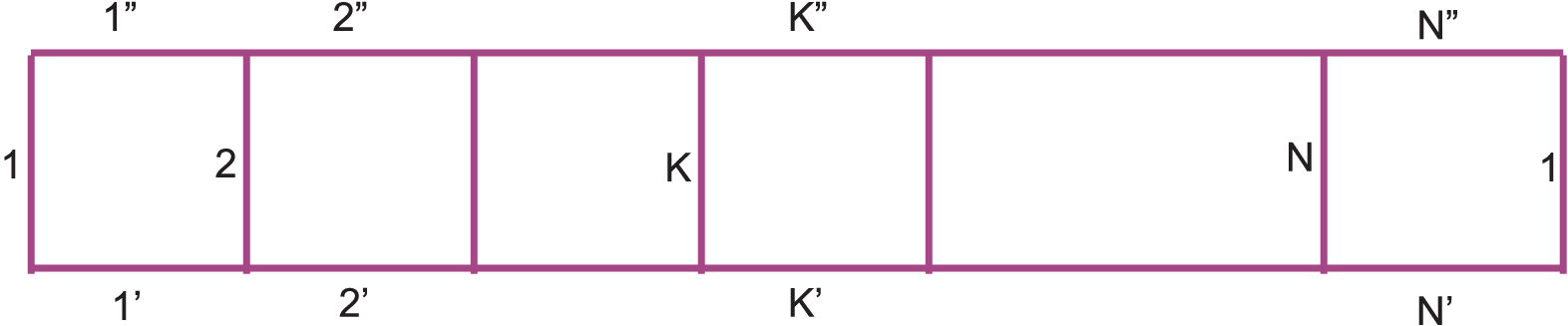
Consider a two-leg ladder network with length with the labeling of links as shown in figure (1), where we use the superscripts and to denote the vertices pertaining to the lower and upper legs. For this ladder, the vertex and plaquette operators take the following form,
| (2) |
Throughout the paper, we use the generic names and for pointing to general vertex and plaquette operators in a network and the names indicated in Eq. (2) for pointing to specific operators in the ladder. For a closed surface the operators in (1) are constrained by the relations , however for the ladder, which is a surface with two boundaries, the second constraint does not hold and we are left with
| (3) |
Therefore the operators in (2) are commuting operators in the dimensional Hilbert space of the ladder. They all commute with the Hamiltonian and hence the ground state is two-fold degenerate. The following non-local operators play an important role.
| (4) |
It can be clearly seen that they commute with each other and also with the Hamiltonian,
| (5) |
They correspond to a cycle around the ladder. Both of them square to 1 and hence have eigenvalues . As we will see the operator generates the two-fold degeneracy of the ground state.
2.1 The ground and the top states
It is clear from (1) that the ground state is a state with the property
| (6) |
To find the explicit form of the ground state, we use the property which is equivalent to and introduce the state
| (7) |
where , is a product of all spins in the direction. Note that and . It is obvious that satisfies the condition (6) and hence is a ground state. The other ground state is obtained from by the action of the operator which corresponds to the only nontrivial homology cycle of the surface, that is and form the doubly degenerate ground states of the model,
| (8) |
Note that , being a cycle, cannot be expressed as any
combination of product of plaquette operators , which are all
homologically trivial. This shows that the two states and are independent.
The top state, the state with the highest energy is one which is an eigenstate of all the vertex and plaquette operators with eigenvalues . It can be readily verified that the following state is such an state:
| (9) |
where is the product of all spins in the direction in the network. The other degenerate state is obtained by the action of the operator , i.e. The highest energy will be
| (10) |
2.2 The complete spectrum
We can now construct the full spectrum. To this end we note that for any arbitrary state , the state,
is an eigenstate of all the plaquette operators, with eigenvalues . The reason is the relation . Hereafter we use the abbreviation for such a string of operators,
| (11) |
These operators satisfy
| (12) |
To construct states which are eigenstates of the vertex operators and at the same time be independent, let us define the following operators
| (13) |
where the sequence of and are 0 or 1 and the labeling are those shown in figure (1). Figure (6 ) shows the links which contribute to the construction of such operators. It is important to note that the links of only one leg are among this set. Now let us define
| (14) |
The operators in (13) have simple commutation relations with the vertex and plaquette operators. One can verify the following relations
| (15) | |||||
| (16) | |||||
| (17) |
This leads to
| (18) | |||||
| (19) | |||||
| (20) |
The above relations indicate that the states thus constructed are eigenstates of Hamiltonian,
| (21) |
where the energy is found from (1) and (18) to be
| (22) |
In terms of Ising-like variables, and which take values , the energy can be rewritten in the form
| (23) |
In the sequel we will use both the indices and where no confusion arises. The states have binary indices and hence the number of such states is exactly equal to the dimension of the Hilbert space, hence they will comprise the full energy spectrum, provided that we can show they are independent. To investigate this question, let us look at the inner product of these states.
| (24) | |||||
| (25) |
We now note that the operators generate only open or a homologically trivial loop, while the operator only generate homologically trivial loops, and hence the above matrix element vanishes unless . Moreover by expanding it is clearly seen that . Hence we find
.
The independence of these states and the equality of their number with the dimension of Hilbert space, indicates that they comprise the complete spectrum of the Hamiltonian. It is also instructive to note the symmetry of the spectrum. If we indicate by the binary complement of the indices (i.e. ) and similarly for other indices, we find from (22) that
| (26) | |||||
| (27) |
The first relation expresses the two-fold degeneracy which is the result of the topology of the surface, that is the action of the cycle (4) on any state, produces another state with the same energy. The second relation indicates how the spectrum is affected if we invert the coupling constants and around 0; the spectrum should be inverted around the values . One should also note that only the ground and the top states have two-fold degeneracy and the degeneracy of the other states is much larger.
2.3 The partition function and averages of different observables
From the complete spectrum it is straightforward to calculate the partition function. One writes
| (28) | |||||
| (29) |
where the last equality defines the partition functions and . It is obvious that . Using a transfer matrix, we find
| (30) |
The full partition function is therefore given by
| (31) |
In the thermodynamic limit, the average energy is obtained from the partition function to be:
| (32) |
In the same limit the entropy is found from to be
| (33) |
The entropy can be written as a sum of two terms, namely , where the first one is the contribution of the vertex terms and the other is the contribution of plaquette terms, and
| (34) | |||||
| (35) |
Figure (2) shows the total entropy as a function of and .

An interesting non-local observable is the string operator defined in (4). One finds
| (36) |
Passing through , one finds
| (37) |
where we have used the commutation relations of the operators and also the fact that ( ) and consequently Inserting this into (36) one arrives at
| (38) |
where again an appropriate transfer matrix gives the final result
| (39) |
In the thermodynamic limit this gives
| (40) |
which shows a phase transition at zero temperature. It is easy to see that at all temperatures.
3 Reduced density matrices and entropies of different subsystems
In this section we derive the reduced density matrices of different
subsystems at finite temperature. These subsystems are denoted by
(the spins on one of the legs of the ladder), (the spins of
the totality of all the rungs of the ladder), and (the spins of
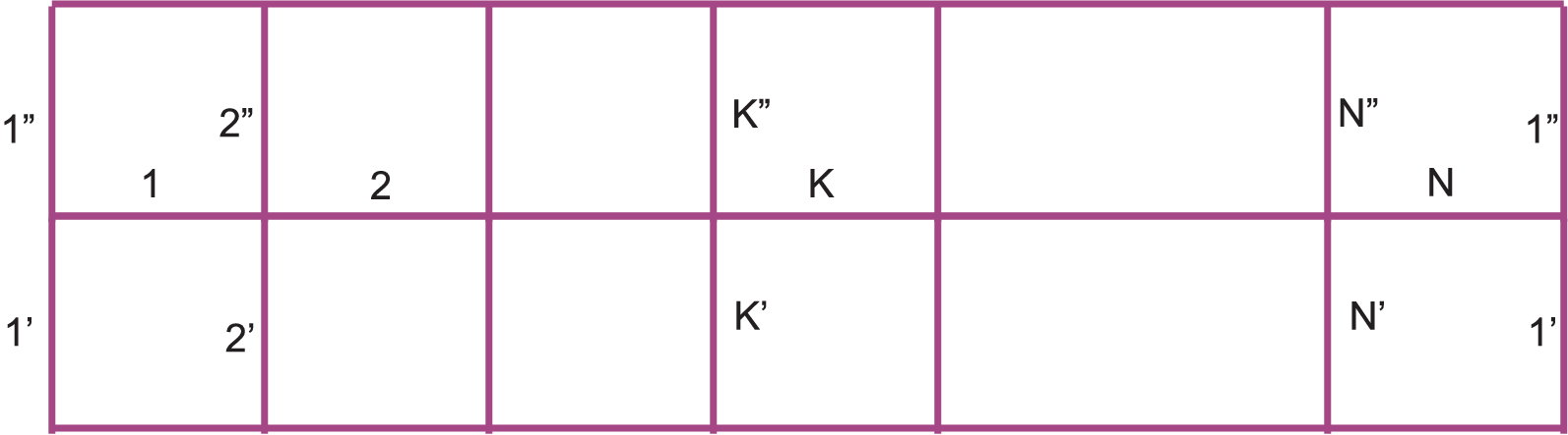
a subset of the rungs), see figure (3). The
significance of the subsystems and is that corresponds
to a topologically nontrivial loop in the surface, while
corresponds to a trivial curve and one expects that this difference
of topology shows itself in the entropy of these subsystems. As we
will show, this is indeed the
case.
To prepare ourself for the calculation of the reduced density matrix
at finite temperatures, in each case we first derive the reduced
density matrix of the relevant subsystem when the whole system is
at the state
. The corresponding density matrices will be denoted by and . This will pave the way for determination of
the reduced density matrices at arbitrary temperatures which will be denoted by and . We also use the notation to denote the
restriction of the product state to the subsystem with similar notations for and .
3.1 Subsystem A: One leg of the ladder
We have
| (41) |
where for any subset , means that we take the trace over the complement of .

To calculate the trace, we note that the state can be written as follows
| (42) |
where the indices take the values 0 or 1. We now use the fact that and take the trace over the product of the operators to arrive at
| (43) | |||||
| (44) |
where
| (45) |
From the above equation we find
| (46) |
which when inserted into (43) this gives
| (47) | |||||
| (48) |
This shows among other things that at zero temperature, each of the
two legs of the ladder are in a maximally mixed state. The
interesting point is that this situation persists at all
temperatures. To see this, we take the upper leg as our subsystem
, since in this case, the analysis will be greatly simplified.
Since the system is symmetric, whatever we obtain will also be valid
for the lower leg. We have
| (49) |
The reason for taking to be the upper leg of the ladder is that we could pass through the operator cyclically within the trace and arrive at the simple result that Obviously any subsystem of will also be in a maximally mixed state.
3.2 Subsystem B: All the rungs of the ladder
Consider now subsystem , the full set of rungs of the ladder. We first derive the reduced density matrix , when the whole ladder is in the state . Using the decomposition (42) and the structure of the operators (2), we find
| (50) |
where
| (51) |
and
| (52) |
Using the fact that , and inserting the result in (50), noting the two-to-one correspondence between the indices and the powers of and rearranging terms, we obtain
| (53) |
where
| (54) |
Note that this is independent of the index set of the state . Also in each state the flip operators come in pair, so this state is an even parity state, i.e. a state where an even number of spins have been flipped from + to -. The state is thus a uniform mixture of all even parity states. Call this density matrix . Let us now consider finite temperatures, for which we have to calculate
| (55) |
where . The reduced density matrix at finite temperature will now be given by
| (56) |
From the above definition of , and that of and , one finds that
| (57) |
where is the uniform mixture of odd-parity states and denotes the degree of , i.e.
Inserting this into (56) yields
| (58) |
Using the expression of the parity and Eqs. (36) and (37) we find the following simple expression
| (59) | |||||
| (60) |
where use has been made of the fact that . The entropy of this state, which is a mixture of orthogonal states, can now be readily calculated. A straightforward calculation gives
| (61) |
where is the Shannon entropy function.

Figure (4) shows for several values of system sizes . In the thermodynamic limit, there is a sharp rise in this quantity only at zero temperature, but for finite , it is also seen that there is an almost sharp rise at finite temperatures.
3.3 Subsystem C: A subset of the rungs
Once the density matrix of the subsystem B is obtained, we can trace out any number of the rungs to find the reduced density matrix of the remaining subset of rungs. Using (59) and noting that on taking the trace over any subsystem, the contribution of and cancel each other, one arrives at the simple result that
| (62) |
where is any proper subset of the rungs and is the size of this subset. It is interesting to note that how the topology of the surface is reflected in the entropy of its subsystems.
3.4 Thermal entanglement of two spins
From the reduced density matrices found in previous subsections, we know that any two spins on a leg of the ladder are in a maximally mixed state and hence there is no thermal entanglement between such spins. The same is true between any two spins on the rungs of the ladder. In fact it has been shown [27] that in the ground state, there is no entanglement between any two qubits. However one can ask if at higher temperature some degree of entanglement is caused by thermal fluctuations. This indeed happens in some spin systems, below a certain threshold temperature. To investigate this, we compute the reduced density matrices of the two spins, say 1’ and 1” in figure (3) on the two legs, opposite to each other. Call this subsystem . The first step is to calculate which is equal to
. In calculating the trace, one can use the cyclic property of the trace and move around all the terms except the term (which acts nontrivially on the space ) and use the property which after some algebra gives
| (63) | |||||
| (64) | |||||
| (65) |
where in the second line we have used the fact that the closed loops generated by any of ’s cannot be compensated by to make a non-vanishing trace and the third line is the result of explicit expansion and calculation. We will then have
| (66) |
Acting the operators on both sides and performing the above simple calculation with the help of the transfer matrix, we find that , which means that there is no thermal entanglement between these two spins.
4 The complete spectrum of the three-leg ladder
What has been done for the two-leg ladder can be extended to three-leg ladder, Fig.(5), without much effort. The first step is to define the states
| (67) |
and then the trick is to find a suitable generalization for the operators , so that their action on the above state, produces the correct number of independent eigenstates of the vertex operators. The suitable generalization is as follows
| (68) |
where the flipping operators correspond to the links shown in Fig. (6).
One can now easily verify the following commutation relations, where we use and for vertex operators on site for the lower, middle and upper legs of the ladder respectively:
| (69) | |||||
| (70) | |||||
| (71) |
One can proceed along the same way as detailed in section (2) for the two-leg ladder and show that the states are energy eigenstates with energies given by
| (72) |
where again we have used Ising-like variables, i.e. instead of the binary variables. Moreover the number of these states is which is equal to the dimension of the Hilbert space and they are orthogonal. (See the reasoning following Eq. (24)).

The basic point is that every conceivable combinations of the flipping operators in , corresponding to Fig. (6) when acting on , will produce only open or homologically trivial loops of negative spins which will certainly be orthogonal to the state generated by acting on . The partition function turns out to be
| (73) |
5 Discussion
We have determined the complete spectrum of the Kitaev model on a
spin ladder and from there we have determined the reduced density
matrices for its various subsystems at finite temperature. We have
shown that on two and three-leg ladders, the model is equivalent to
particular types of one dimensional classical Ising models, models
with different spins on the sites and links.
To what extent this study can be pursued for the two dimensional
lattice,( i.e. a torus)? On a lattice with sites, and
links, the Hilbert space dimension is . We can already
construct (un-normalized) states of the form which are energy
eigenstates. To find more states, we have to find subsets of
flipping operators and then construct operators of the form
and energy eigenstates as
.
The subset should have the following important property: when
acting on , no combination of links in should be
able to generate a homologically trivial loop of negative spins on
the lattice. Let be a maximal set of this type with
elements. Then the total number of independent energy
eigenstates found in this way is .
For the square lattice of sites, one such set is shown in Fig.
(7), where . In fact is
nothing but a one-cycle which goes back and forth around the torus,
but does not wrap around it, and comprises half of the links on the
network. We call the maximal cycle, since it is the cycle which
contains the maximal set of links (the addition of any link to this
cycle will make a trivial loop out of it), or the excitation curve,
since flipping operators chosen from it, and acting on create all the excited states.
Since , the states constructed as form the whole set of energy eigenstates. Numbering the links along the bold-face curve shown in figure (7), in a consecutive way from to , shows that the energy of such a state is equal to , where we have used the Ising type labels and instead of the binary labels and . This leads to the partition function
| (74) |
Remark: We could have taken just such a canonical curve for
the two and three leg ladders, instead of the ones shown in figure
(6), although it may have rendered the calculations of
reduced density matrices in these simple cases unnecessarily
involved. The curves shown in fig (6) can be obtained
from this canonical curve by the moving up and down the horizontal
links appropriately which amounts to application of plaquette
operators. Such plaquette operators affect the eigenstate by only a
phase.

Knowing the full spectrum in this way, will enable us to study the
entanglement and many other properties of the Kitaev model in
detail. Furthermore this knowledge may be useful in other more
detailed studies of the Kitaev model, where the dynamics of the
model is required. For example in the study of dynamics of classical
and quantum phase transitions in systems with topological order,
mentioned in the introduction [30]. Another interesting
context is the study of auto-correlation times of the toric code,
which is related to the important problem of how long quantum
information can be protected in topological degrees of freedom in a
background of inevitable thermal fluctuations. This later problem
was first addressed in [32, 33] in which among other
things, a mapping of the spectrum of the Kitaev model
to two uncoupled Ising chains were found.
Another important problem which may be treated in an alternative way by the characterization of spectrum in the way shown in this paper, is the problem of sustainment of topological order at finite temperatures. This problem has been studied in a number of works,[24, 34, 35] using a different description of the spectrum.
6 Acknowledgements
I would like to thank Miguel Martin-Delgado for his very valuable comments and a critical review of the manuscript.
References
- [1] E. H. Lieb, T. Schultz and D. Mattis, Annals of Physics16407 (1966).
- [2] E. H. Lieb and D. C. Mattis Mathematical Physics in One Dimension Academic Press, New York 1966.
- [3] R. J. Baxter Exactly Solved Models in Statistical Mechanics, Academic Press, London,1982.
- [4] M. Fannes, B. Nachtergaele and R. F. Werner, Europhys. Lett. 10 633, (1989), A. Klumper, A. Schadschneider, J. Zittartz, J. Phys. A 24 L955 (1991); Z. Phys. B, 87, 281 (1992).
- [5] A. Klümper, A. Schadschneider and J. Zittartz, Europhys. Lett.24293 (1993); M. A. Ahrens, A. Schadschneider and J. Zittartz, Europhys. Lett 59, 889, 2002.
- [6] E. Bartel, A. Schadschneider and J. Zittartz, Eur. Phys. Jour. B 31, 209 2003.
- [7] M. Asoudeh, V. Karimipour and A. Sadrolashrafi, Phys. Rev. B 75, 224427 2007; Phys. Rev. A 76,012320(2007); Phys. Rev. B 76,064433(2008).
- [8] S. Alipour, V. Karimipour and L. Memarzadeh, Phys. Rev. A 75052322(2007), Eur. Phys. J. B. 62, 159-169, (2008).
- [9] V. Karimipour and L. Memarzadeh, Phys. Rev. B 77, 094416 (2008).
- [10] S. Alipour, S. Baghbanzadeh, and V. Karimipour, Europhysics Letters (EPL), 84 67006 (2008).
- [11] M. A. Nielsen, and I. L. Chuang;Quantum computation and quantum information,Cambridge University Press, Cambridge, 2000.
- [12] A. Osterloh, L. Amico, G. Falci, and R. Fazio, Nature 416, 608 (2002).
- [13] T. J. Osborne, and M. A. Nielsen, Phys. Rev. A 66, 032110 (2002).
- [14] A.Yu.Kitaev, Annals of Physics 303 no. 1, 230 (2003).
- [15] A. Kitaev and J. Preskill, Phys. Rev. Lett. 96, 110404 (2006).
- [16] H. Bombin, M.A. Martin-Delgado, Phys.Rev.Lett. 97 180501 (2006); Phys.Rev.Lett. 98 160502, (2007); Phys.Rev. B78 115421,(2008).
- [17] H. Bombin, M. Kargarian, and M.A. Martin-Delgado, ”Interacting Anyonic Fermions in a Two-Body ‘Color Code’ Model” preprint arXiv:0811.0911; M. Kargarian, Phys. Rev. A 78, 062312 (2008).
- [18] J. K. Pachos, Ann. of Phys. 6, 1254 (2006); Int. Jour. Quant. Information, Vol. 4, No. 6, 947-954 (2004).
- [19] M. H. Freedman, A. Yu. Kitaev, and Z. Wang, Commun.Math.Phys. 227 587-603, (2002); M. Freedman, M. Larsen, and Z. Wang, Comm.Math. Phys. 227 605622, (2002); M. H. Freedman, A. Kitaev, M. J. Larsen, and Z. Wang, Math. Soc. 40 31-38, (2003).
- [20] C. Nayak, S. H. Simon, A. Stern, M. H. Freedman, and S. D. Sarma, , Non-Abelian Anyons and Topological Quantum Computation, preprint, arXiv:0707.1889.
- [21] G. Kells, et. al., Phys.Rev.Lett. 101240404, (2008);
- [22] Ville et. al., Annals of Physics, Volume 323,9, 2286 (2008);
- [23] A Kitaev, Ann. Phys. (N.Y.) 321, 2 (2006); H. D. Chen and Z. Nussinov, J. Phys. A 41, 075001 (2008); D. H. Lee, G.-M. Zhang, and T. Xiang, Phys. Rev. lett. 99, 196805 (2007).
- [24] C. Castelnovo and C. Chamon, Phys. Rev. B 76, 184442 (2007); Phys. Rev. B 76, 174416 (2007).
- [25] S. Dusuel, K. P. Schmidt, and J. Vidal, Phys. Rev. Lett. 100, 177204 (2008); K. P. Schmidt, S. Dusuel, and J. Vidal, Phys. Rev. Lett. 100, 057208 (2008).
- [26] H. Bombin, and M.A. Martin-Delgado, Phys. Rev. A 77, 042322 (2008).
- [27] A. Hamma, R. Ionicioiu, and P. Zanardi, Phys.Lett. A 337, 22 (2005); A. Hamma, R. Ionicioiu, and P. Zanardi, Phys.Rev. A 72, 012324 (2005).
- [28] M. Kargarian, Phys. Rev. A 78, 062312 (2008).
- [29] T. W. B. Kibble, J. Phys. A 9, 1387 (1976); W. H. Zurek, Nature 317, 505 (1985).
- [30] A. Bermudez, D. Patanè, L. Amico, and M. A. Martin-Delgado, Phys. Rev. Lett. 102, 135702 (2009).
- [31] M. Creutz, Phys. Rev. Lett 83, 2636 (1999).
- [32] Zohar Nussinov and Gerardo Ortiz, Annals of Physics, 324, 5, (2009).
- [33] Zohar Nussinov and Gerardo Ortiz, Phys. Rev. B 77, 064302 (2008).
- [34] S. Iblisdir, D. Perez-Garcia, M. Aguado, J. Pachos, PRB 79, 134303 (2009).
- [35] S. Iblisdir, D. Perez-Garcia, M. Aguado, J. Pachos, ”Thermal states of anyonic systems”, arXiv:0812.4975 .