In this section we adapt an argument given in [5] to the context of the $AdS_{4}/CFT_{3}$ correspondence in M-theory. Our goal is to confirm that the linearized solution presented in the previous section indeed corresponds to sourcing the operator ${\cal O}_{2}$ dual to the field $\phi$ on a 1+1-dimensional interface/defect, instead of sourcing ${\cal O}_{2}$ on the entire 2+1-dimensional boundary. The metric for the $AdS_{3}$ slicing of $AdS_{4}$ takes the following form near $\mu=\pm\pi/2$.

	$\displaystyle ds^{2}$	$\displaystyle=$	$\displaystyle{1\over\cos^{2}\mu}\Big(d\mu^{2}+{1\over z^{2}}(-dt^{2}+dx^{2}+dz^{2})\Big)$		(2.8)
		$\displaystyle=$	$\displaystyle{1\over z^{2}\cos^{2}\mu}\Big(z^{2}d\mu^{2}+(-dt^{2}+dx^{2}+dz^{2})\Big)$

It is now easy to see that the boundary of $AdS_{4}$ in this coordinate system consists of three components [2]. The limits $\mu\to{\pm}\pi/2$ correspond to two 2+1-dimensional half spaces (since the range of $z$ is the positive real numbers). The two half spaces are glued together along a 1+1-dimensional interface/defect which is associated with the boundary of the $AdS_{3}$ slice and is reached as $z\to 0$ with $\mu$ arbitrary. With the definition $\epsilon=|\cos(\mu)|z$, the boundary components are reached uniformly as $\epsilon\to 0$. The boundary source for an operator ${\cal O}_{2}$ can be obtained by isolating the term in $\phi$ which scales like $\epsilon^{3-\Delta}$.

	$\displaystyle\phi_{source}$	$\displaystyle=$	$\displaystyle\lim_{\epsilon\to 0}\left(\epsilon^{\Delta-3}\phi(\mu)\right)$		(2.9)
		$\displaystyle=$	$\displaystyle\lim_{\epsilon\to 0}\left({|\cos(\mu)|\over z}\phi_{2}\right)$

The limits depends upon the direction along which $\varepsilon=0$ is being approached. As one keeps $z\not=0$ fixed, and takes $\mu\to\pm\pi/2$, the two half spaces $\mu=\pm\pi/2$ are approached away from the interface/defect. It follows from (2.9) that this limit, and thus the source for the ${\cal O}_{2}$ operator, vanishes. This means the dual operator ${\cal O}_{2}$ is not inserted in the boundary CFT away from the interface/defect.

The interface/defect is approached as one takes $z\to 0$ with $\mu\neq\pm\pi/2$. In this case the limit in (2.9), and thus the source for the ${\cal O}_{2}$ operator, diverges. This behavior indicates the presence of a Dirac $\delta$-function source for the operator ${\cal O}_{2}$ on the 1+1-dimensional interface/defect. This may be established directly by integrating $\phi_{source}$ over a small disk around $\epsilon=0$ in the $z,\mu$-plane. The corresponding integral is given by $\int d\mu\;dz\,z\;\phi_{source}$ and is finite. Its interpretation is that a term which has $\delta$-function support on the interface/defect is being added to the Lagrangian of the 2+1-dimensional CFT,

$${\cal L}={\cal L}_{CFT_{3}}+\lambda\;\delta(x^{\perp}){\cal O}_{2}$$

(2.10)

where $x^{\perp}$ is the coordinate transverse to the 1+1-dimensional interface/defect. The linearized analysis corresponds to a small perturbation with $\lambda\ll 1$. Since the conformal dimension of the operator ${\cal O}_{2}$ is two, its addition to ${\cal L}_{CFT_{3}}$ preserves the (global) 1+1-dimensional conformal symmetry of the interface/defect, but breaks the full 2+1-dimensional conformal symmetry of the CFT.

In this subsection, we shall inspect the supergravity fields on $AdS_{4}\times S^{7}$ and identify viable candidates for the pseudo-scalar deformations studied above. The spectrum of the Kaluza-Klein (KK) compactification of M-theory on $AdS_{4}\times S^{7}$ has been obtained by [21, 22]²² 2 See [23] for a dictionary between supergravity and AdS/CFT conventions.. One gets infinite towers of KK-states organized in representations of the $SO(8)$ R-symmetry group, as collected in Table 1.

There exists a consistent truncation of the theory to the “massless” ${\cal N}=8$ multiplet which produces ${\cal N}=8$ gauged supergravity in four dimensions and is given by the representations with $n=0$, summarized in Table 2.

Note that the 70 scalars of gauged supergravity split into 35 scalars (denoted $0^{+}$ in Table 2) and 35 pseudo-scalars scalars (denoted by $0^{-}$). In the KK-reduction the scalars are obtained from the reduction of the metric component on the sphere whereas the pseudo-scalars are obtained from the AST field strength on the sphere. As discussed in section 2, the ambiguity for the conformal dimensions for the operators dual to the (pseudo-) scalars was resolved in [19, 20] and leads to the values displayed in Table 2.

In gauged ${\cal N}=8$ supergravity a Janus interface/defect configuration can be obtained applying the linearized analysis of section 2 for a pseudo-scalar transforming in the ${\bf 35_{c}}$ representation of the $SO(8)$ R-symmetry. This field should be dual to a dimension 2 operator in the $CFT_{3}$ defined by the decoupling limit of a large number of M2-branes.

In principle one could try to solve the equations of motion for the ${\cal N}=8$ gauged supergravity and a Janus Ansatz to obtain a fully non-linear solution dual to the insertion of such an operator. Solving the full second order equations of motion is, however, prohibitively complicated. A different approach is to ask wether there are interface/defect solution which preserve some of the 32 supersymmetries and correspond to superconformal interface/defects. Solving the resulting BPS-equation is generically easier than solving the equations of motion.

Note that the ${\bf 35_{c}}$ representation can be characterized as the rank four self-dual antisymmetric tensor representation of $SO(8)$. Turning on such a field will therefore break the $SO(8)$ R-symmetry down to $SO(4)\times SO(4)$. Hence one expects the resulting theory to have $SO(4)\times SO(4)$ unbroken R-smmetry.

In the following we will use the results of [24] to obtain a solution of 11-dimensional supergravity, which preserves sixteen supersymmetries, is locally asymptotic to $AdS_{4}\times S^{7}$, preserves $SO(2,2)\times SO(4)\times SO(4)$ symmetry and has all the characteristics of a fully non-linear and back-reacted interface/defect solution discussed above.

In [24], the BPS equations governing half-BPS solutions were reduced to constructing a Riemann surface $\Sigma$ with boundary, a real positive harmonic function $h$ on $\Sigma$, and the solution to a first order partial differential equation on $\Sigma$ for a complex-valued field $G$, subject to a point-wise quadratic constraint. The partial differential equation for $G$ is given by,

$\displaystyle\partial_{w}G={1\over 2}(G+\bar{G})\partial_{w}\ln h$

(3.4)

for an arbitrary complex coordinate system $w,{\bar{w}}$ on $\Sigma$. For solutions which are locally asymptotic to $AdS_{4}\times S^{7}$ (referred to as “case I” in [24]), the field $G$ is subject to the following point-wise quadratic constraint,

$\displaystyle|G(w,{\bar{w}})|^{2}\geq 1\qquad\qquad{\rm for~all}~(w,{\bar{w}})\in\Sigma$

(3.5)

We define the following function $W$ on $\Sigma$,

$\displaystyle W^{2}\equiv 4|G|^{4}+(G-\bar{G})^{2}$

(3.6)

Assuming that the point-wise quadratic constraint $|G|^{2}\geq 1$ is obeyed, we automatically have $W^{2}\geq 0$, so that $W$ is real. The special value $W^{2}=0$ corresponds to either $G=+i$ or $G=-i$. The metric factors in (3.1) are then expressed as follows,,

	$\displaystyle f_{1}^{6}$	$\displaystyle=$	$\displaystyle{h^{2}W^{2}\over 16^{2}(|G|^{2}-1)^{2}}$
	$\displaystyle f_{2}^{6}$	$\displaystyle=$	$\displaystyle{h^{2}(|G|^{2}-1)\over 4\,W^{4}}\left(2|G|^{2}+i(G-\bar{G})\right)^{3}$
	$\displaystyle f_{3}^{6}$	$\displaystyle=$	$\displaystyle{h^{2}(|G|^{2}-1)\over 4\,W^{4}}\left(2|G|^{2}-i(G-\bar{G})\right)^{3}$		(3.7)

The metric factor $\rho$ in (3.3) is given by,

$\displaystyle\rho^{6}$

$\displaystyle=$

$\displaystyle{\left|\partial_{w}h\right|^{6}\over 16^{2}h^{4}}\big(|G|^{2}-1\big)W^{2}$

(3.8)

The anti-symmetric tensor field-strengths are expressed in terms of $g_{1a},g_{2a}$, and $g_{3a}$. They can be simply related to currents $\partial_{w}b_{1}$, $\partial_{w}b_{2}$, and $\partial_{w}b_{3}$, on $\Sigma$, which are conserved as a result of the Bianchi identities, and are given as follows,

	$\displaystyle(f_{1})^{3}g_{1w}=-\partial_{w}b_{1}$	$\displaystyle=$	$\displaystyle-{3W^{2}\partial_{w}h\over 32G(|G|^{2}-1)}-{1+|G|^{2}\over 16G(|G|^{2}-1)^{2}}\,J_{w}$
	$\displaystyle(f_{2})^{3}g_{2w}=-\partial_{w}b_{2}$	$\displaystyle=$	$\displaystyle-{(G+i)\left(2|G|^{2}+i(G-\bar{G})\right)^{2}\over W^{4}}\,J_{w}$
	$\displaystyle(f_{3})^{3}g_{3w}=-\partial_{w}b_{3}$	$\displaystyle=$	$\displaystyle+{(G-i)\left(2|G|^{2}-i(G-\bar{G})\right)^{2}\over W^{4}}\,J_{w}$		(3.9)

where the following intermediate quantity was used for notational compactness,

$\displaystyle J_{w}={1\over 2}(G\bar{G}-3\bar{G}^{2}+4G\bar{G}^{3})\partial_{w}h+hG\partial_{w}\bar{G}$

(3.10)

It was shown in [24] that the equations of motion of as well as the Bianchi identities are satisfied for any harmonic $h$ and any $G$ which solves (3.4).

The simplest solution is the maximally symmetric $AdS_{4}\times S^{7}$ itself. The corresponding Riemann surface is the infinite strip,

$\displaystyle\Sigma=\{w\in{\bf C},~w=x+iy,~x\in{\bf R},\;0\leq y\leq\pi/2\}$

(3.11)

Note that the Riemann surface $\Sigma$ has two boundary components, namely $y=0$ and $y=\pi/2$. In these coordinates, the functions $h$ and $G$ for the $AdS_{4}\times S^{7}$ solution are given by,³³ 3 For simplicity, we shall exhibit the solutions with unit $AdS_{4}$-radius. The solution for general $AdS_{4}$-radius $R_{0}$ may be obtained by scaling $h\to R_{0}^{3}h$, while leaving $\Sigma$, $w,\bar{w}$, and $G$ unchanged. As a result, the metric factors scale as follows, $f_{i}\to R_{0}f_{i}$, $\rho\to R_{0}\rho$, while the flux fields scale as $b_{i}\to R_{0}^{3}b_{i}$ for $i=1,2,3$.

	$\displaystyle h$	$\displaystyle=$	$\displaystyle 4i\big({\rm\,sh}(2w)-{\rm\,sh}(2\bar{w})\big)$
	$\displaystyle G$	$\displaystyle=$	$\displaystyle i{{\rm\,ch}(w+\bar{w})\over{\rm\,ch}(2\bar{w})}$		(3.12)

It is easy to check that the partial differential equation (3.4) as well as the point-wise quadratic constraint (3.5) are satisfied. Using (3.7), the metric factors become,

$\displaystyle f_{1}={\rm\,ch}(2x)\qquad f_{2}=2\cos(y)\qquad f_{3}=2\sin(y)\qquad\qquad\rho=1$

(3.13)

The boundary may be characterized by the vanishing of the harmonic function $h=0$, or alternatively, by $G=\pm i$. On the lower boundary of the strip $\Sigma$ where $y=0$ one has $G=+i$, which implies that the radius $f_{2}$ of $S_{2}^{3}$ vanishes. On the upper boundary of the strip $\Sigma$ where $y=\pi/2$ one has $G=-i$, which implies that the radius $f_{3}$ of $S_{3}^{3}$ vanishes. The boundary of $AdS_{4}$, on the other hand, is located at $x=\pm\infty$.

It turns out that there is a simple deformation of $AdS_{4}\times S^{7}$ (reviewed in the previous section) which corresponds to a Janus solution in M-theory. As before, the holomorphic coordinate is denoted as $w=x+iy$ and the strip is parametrized as (3.11). The harmonic function $h$ is taken to be proportional to the one of (3.12), but is rescaled in order for the asymptotic $AdS_{4}\times S^{7}$ solution to have the same radius as the undeformed solution (3.12), namely with unit $AdS_{4}$-radius,

$$h={4i\over\sqrt{1+\lambda^{2}}}\Big({\rm\,sh}(2w)-{\rm\,sh}(2\bar{w})\Big)$$

(3.14)

The expression for $G$ is given by

$\displaystyle G=i{{\rm\,ch}(w+{\bar{w}})+\lambda{\rm\,sh}(w-{\bar{w}})\over{\rm\,ch}(2{\bar{w}})}$

(3.15)

It is easy to check that the partial differential equation (3.4) as well as the positivity constraint (3.5) are satisfied for any real value of $\lambda$. The solution forms a one-parameter deformation of $AdS_{4}\times S^{7}$, which one recovers by setting $\lambda=0$.

The metric factors can be expressed concisely in terms of two functions,

	$\displaystyle F_{+}(x,y)$	$\displaystyle=$	$\displaystyle 1+2\lambda\Big({\rm\,sh}(2x)+\lambda\Big)\cos^{2}(y)/{\rm\,ch}^{2}(2x)$
	$\displaystyle F_{-}(x,y)$	$\displaystyle=$	$\displaystyle 1-2\lambda\Big({\rm\,sh}(2x)-\lambda\Big)\sin^{2}(y)/{\rm\,ch}^{2}(2x)$		(3.16)

The metric factors (3.7) become,

	$\displaystyle f_{1}$	$\displaystyle=$	$\displaystyle{{\rm\,ch}(2x)\over\sqrt{1+\lambda^{2}}}F_{+}(x,y)^{1\over 6}F_{-}(x,y)^{1\over 6}$
	$\displaystyle f_{2}$	$\displaystyle=$	$\displaystyle 2\cos(y)\,F_{+}(x,y)^{1\over 6}F_{-}(x,y)^{-{1\over 3}}$
	$\displaystyle f_{3}$	$\displaystyle=$	$\displaystyle 2\sin(y)\,F_{-}(x,y)^{1\over 6}F_{+}(x,y)^{-{1\over 3}}$
	$\displaystyle\rho$	$\displaystyle=$	$\displaystyle F_{+}(x,y)^{1\over 6}F_{-}(x,y)^{1\over 6}$		(3.17)

Note that the metric factor for the base space $\Sigma$ becomes non-trivial for the deformed solution. Another interesting feature of this solution is that the size of each three sphere at the part of the boundary where it does not vanish, i.e. $y=0$ for $f_{2}$ and $y=\pi/2$ for $f_{3}$, becomes $x$ dependent in contrast to the $AdS_{4}\times S^{7}$ solution where it is constant.

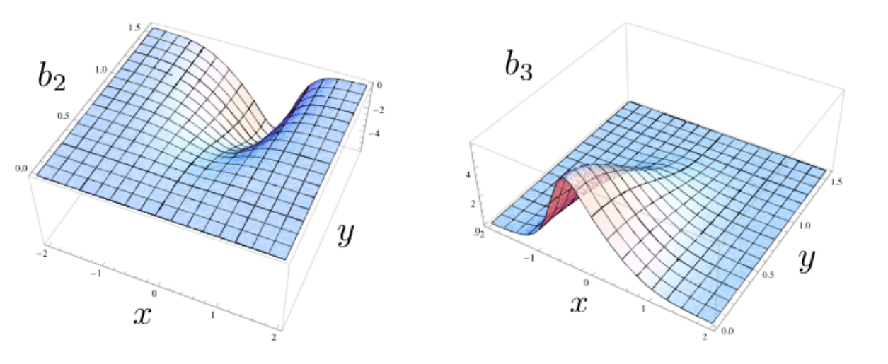
The AST fields along the two three spheres are non-vanishing for the deformed solution. The formulae for the fieldstrengths (3.9) can be integrated and one obtains the following expressions for the AST potentials.

	$\displaystyle b_{2}$	$\displaystyle=$	$\displaystyle-{8\lambda\sqrt{1+\lambda^{2}}\sin^{4}(y)\over{\rm\,ch}^{2}(2x)\;F_{-}(x,y)}$
	$\displaystyle b_{3}$	$\displaystyle=$	$\displaystyle{8\lambda\sqrt{1+\lambda^{2}}\cos^{4}(y)\over{\rm\,ch}^{2}(2x)\;F_{+}(x,y)}$		(3.18)

The explicit formulae for the AST potential $b_{1}$ are also easy to calculate but will not be needed in the following. We have checked that the solutions indeed satisfies all equations of motion of 11-dimensional supergravity. The solution preserves sixteen of the thirty two supersymmetries by construction [24].

In the previous section we utilized the coordinate system in which $\Sigma$ is a strip parametrized as $\Sigma=\{(x,y),x\in{\bf R},\;0\leq y\leq\pi/2\}$. The boundaries of $\Sigma$ at $y=0,\pi/2$ are the location where the volume of the first and second three sphere vanishes. For fixed $x$ the finite $y$-interval together with the two three spheres produces a deformed seven sphere with $SO(4)\times SO(4)$ symmetry. The asymptotic $AdS$ region is reached by taking $x\to\pm\infty$. In this limit the leading terms of the metric factors (3.17) behave as follows,

$$ds^{2}={1\over 4}e^{\pm 4x}\;{-dt^{2}+ds^{2}+dz^{2}\over z^{2}}+4\sin^{2}(y)\;ds_{S_{2}^{3}}^{2}+4\cos^{2}(y)\;ds_{S_{3}^{3}}^{2}+4(dx^{2}+dy^{2})+o(e^{\mp 4x})$$

(3.19)

which is the asymptotic form of $AdS_{4}\times S^{7}$. The leading terms for the 3-form potential $C_{3}$ in the limit $x\to\pm\infty$ can be obtained from (3.18),

$\displaystyle C_{3}={1\over 16}e^{\pm 6x}\hat{\omega}_{AdS_{3}}-{32\lambda\over\sqrt{1+\lambda^{2}}}e^{\mp 4x}\Big(\sin^{4}(y)\;\hat{\omega}_{S_{2}^{3}}-\cos^{4}(y)\;\hat{\omega}_{S_{3}^{3}}\Big)+o(e^{\mp 2x})$

(3.20)

The first term in (3.20) produces the four form flux supporting the $AdS_{4}\times S^{7}$ solution. The second term vanishes when $\lambda=0$, which corresponds to the undeformed solution. Note that the deformed solution has a nontrivial profile for the AST potential along the spheres, but it is easy to see that the conserved M5-brane charge integrates to zero.

To make contact with the discussion of section 2, we first note that the dependence on the $y$ and sphere coordinates in the second and third terms in (3.20) corresponds to a specific AST spherical harmonic on the sphere. The Kaluza-Klein reduction [21] produces the pseudo-scalar field $\phi$ of mass $m^{2}=-2$ transforming in the ${\bf 35_{c}}$ of the $SO(8)$ R-symmetry.

We can relate the coordinate $x$ which parametrizes the $AdS_{3}$ slicing coordinate in the strip parametrization to the coordinate $\mu$ which was employed in section 2 by,

$$\mu\mp\pi/2=e^{\mp 2x}$$

(3.21)

valid in the limit $x\to\pm\infty$. It follows from (3.20) that the pseudo-scalar field mode associated with the KK reduction of the AST potential has the following behavior,

$$\lim_{\mu\to\pm\pi/2}\phi={\rm constant}\times(\mu\mp\pi/2)^{2}+o(\mu\mp\pi/2)^{4}$$

(3.22)

Consequently, the holographic behavior of $\phi$ is exactly of the type discussed in section 2. The holographic interpretation of our solution is that a dimension two operator which preserved $SO(4)\times SO(4)$ R-symmetry, as well as sixteen supersymmetries, is sourced at a 1+1-dimensional interface/defect.

In the context of BPS Janus solutions in Type IIB the related CFT analysis of supersymmetric interface/defects in ${\cal N}=4$ super Yang Mills was carried out in [11, 12, 25, 26]. It would be interesting to pursue a similar analysis for the M2-brane CFT, where significant progress in the formulation of the theory has been made recently [27, 28, 29]. See [30, 31] for other attempts to obtain Janus like solutions for the M2-brane worldvolume theory.

The supergravity description of ABJM theory is given by the quotient $AdS_{4}\times S^{7}/Z_{k}$ of the maximally symmetric vacuum $AdS_{4}\times S^{7}$ by the cyclic group $Z_{k}$ for $k\geq 1$. Here, $Z_{k}$ acts on $S^{7}$, but does not act on $AdS_{4}$. The action of $Z_{k}$ on $S^{7}$ has no fixed points, and the resulting quotient may be viewed as a line bundle over $CP_{3}$ whose fiber $S^{1}$ has radius $1/k$. The quotient breaks the $SO(8)$ R-symmetry to $SU(4)\times U(1)$.

The action on $S^{7}$ may be rendered more explicit by embedding $S^{7}$ into ${\bf R}^{8}$, and parametrizing ${\bf R}^{8}$ by four complex coordinates $z_{i}$, with $i=1,2,3,4$. The $Z_{k}$ transformation is then defined by $z_{i}\to z_{i}\,e^{2\pi i/k}$ for any integer $k\geq 1$, and the quotient is obtained by identifying the points $z_{i}$ and $z_{i}\,e^{2\pi i/k}$ for all four directions $i=1,2,3,4$.

To construct the ABJM Janus solution, it will be more useful to exhibit the $Z_{k}$ transformations in terms of real coordinates, on which the action of the full $SO(8)$ is manifest. The corresponding representation matrix $\gamma$ in the group $SO(8)$ is then given by $\gamma=e^{2\pi H/k}$, where $H$ is the following generator of the Lie algebra $SO(8)$,

$\displaystyle H=\left(\matrix{H_{2}&0\cr 0&H_{3}\cr}\right)\hskip 57.81621ptH_{2}=H_{3}=\left(\matrix{\varepsilon&0\cr 0&\varepsilon\cr}\right)\hskip 57.81621pt\varepsilon=\left(\matrix{0&-1\cr 1&0\cr}\right)$

(4.1)

The notation $H_{2}$ and $H_{3}$ has been introduced for the following reason. The M-theory Janus solution is characterized by the breaking of the Lie algebra $SO(8)$ to $SO(4)_{2}\oplus SO(4)_{3}$, the two $SO(4)_{i}$ subalgebras being the isometries of the spheres $S_{i}^{3}$ for $i=2,3$ of the Janus solution in (3.1). In the above partition of $H$ into the direct sum of $H_{2}$ and $H_{3}$, the generators are arranged so that $H_{2}\in SO(4)_{2}$, and $H_{3}\in SO(4)_{3}$. As a result, the action of $Z_{k}$ on $S^{7}$ descends to the Janus solution as a $Z_{k}$ action on $S_{2}^{3}$ and $S_{3}^{3}$, whose explicit form is given by the $SO(4)$ Lie group matrices $\gamma_{2}=e^{2\pi H_{2}/k}$ and $\gamma_{3}=e^{2\pi H_{3}/k}$.

The action of $\gamma_{2,3}$ on $S^{3}_{2,3}$ is again without fixed points. Furthermore, the action of $\gamma_{2,3}$ leaves all the other ingredients of the Ansatz of (3.1), (3.2), (3.3), and of the solution functions $h$ and $G$ invariant. Thus, we are guaranteed that the quotient of the M-theory Janus solution by the action of $Z_{k}$ will produce a regular family of solutions, parametrized by the same parameter $\lambda$ as the M-theory Janus was. The only change to the geometry resides in the quotient of $S_{2}^{3}\times S_{3}^{3}$ by $Z_{k}$.

The quotienting of $S^{3}$ by $Z_{k}$ reduces the isometry group from $SO(4)$ to an $SU(2)\times U(1)$ subgroup. Thus, we expect the ABJM Janus solution to have a compact bosonic symmetry group $SU(2)\times SU(2)\times U(1)^{2}$, as well as, of course, the full isometry $SO(2,2)$ of $AdS_{3}$, producing a total bosonic symmetry group

$\displaystyle SO(2,2)\times SO(4)\times U(1)^{2}$

(4.2)

Supersymmetry is also reduced under quotienting by $Z_{k}$, $k\not=1,2$. This reduction is entirely due to the reduction of the number of Killing spinors on $S_{2}^{3}\times S_{3}^{3}$, and proceeds in parallel to the corresponding reduction on $S^{7}$. The 4 independent Killing spinors on $S_{2}^{3}\times S_{3}^{3}$ are reduced to only 3 Killing spinors on $(S_{2}^{3}\times S_{3}^{3})/Z_{k}$. For $AdS_{4}\times S^{7}$, this effect reduces the total number of supersymmetries from 32 to 24, while for the M-theory Janus solution, it reduces the number of supersymmetries from 16 to 12. Given these bosonic and supersymmetries, the corresponding invariance superalgebra of the ABJM Janus solution is readily obtained,

$\displaystyle OSp(3|2,{\bf R})\times OSp(3|2,{\bf R})$

(4.3)

which is a subgroup of the $OSp(4|2,{\bf R})\times OSp(4|2,{\bf R})$ algebra of the M-theory Janus solution.

As pointed out in [32, 33], the spectrum of the KK reduced theory can be obtained by decomposing the KK spectrum of $AdS_{4}\times S^{7}$ with respect to $SU(4)\times U(1)$ and keeping only the zero charge sector of the $U(1)$. For the fields of $N=8$ gauged supergravity in Table 2, this implies the following decompositions of $SO(8)$ representations under its $SU(4)\times U(1)$ subgroup,

	$\displaystyle{\bf 28_{v}}$	$\displaystyle\to$	$\displaystyle{\bf 1_{0}}+{\bf 6_{2}}+{\bf 6_{-2}}+{\bf 15_{0}}$
	$\displaystyle{\bf 35_{v}}$	$\displaystyle\to$	$\displaystyle{\bf 10_{2}}+{\bf\overline{10}_{-2}}+{\bf 15_{0}}$
	$\displaystyle{\bf 35_{c}}$	$\displaystyle\to$	$\displaystyle{\bf 10_{2}}+{\bf\overline{10}_{-2}}+{\bf 15_{0}}$		(4.4)

As a result, out of the 35 pseudo-scalar $0^{-}$ fields transforming in the ${\bf 35_{c}}$ of $SO(8)$ in the KK spectrum, fifteen survive the quotient and transform in the ${\bf 15}$ of $SU(4)$. These fields have mass $m^{2}=-2$ and are dual to dimension 2 operators. The linearized analysis of section one is expected to apply to these states, and it provides further evidence for the existence of Janus-like interface/defect solutions in this theory.

It is possible to characterize the dual operator using the ABJM worldvolume theory. The scalars and fermion fields transform as bi-fundamentals of a $U(N)\times U(N)$ gauge theory. There is an SU(2) doublet of bosons $A_{1},A_{2}$ and fermions $\lambda_{1},\lambda_{2}$ which transform as $(N,\bar{N})$ under $U(N)\times U(N)$ gauge symmetry, whereas a second pair of bosons $B_{1},B_{2}$ and fermions $\chi_{1},\chi_{2}$ transforms as $(\bar{N},N)$. The boson and fermion fields can be assembled into the following multiplets [13, 34, 35],

$$Y^{A}=(A_{1},A_{2},B_{1}^{\dagger},B_{2}^{\dagger})\hskip 72.26999pt\Psi^{A}=(\lambda_{1},\lambda_{2},\chi_{1}^{\dagger},\chi_{2}^{\dagger})$$

(4.5)

which transform in the ${\bf 4}$ representation of $SU(4)$, wheras the conjugate fields $(Y^{A})^{\dagger}=Y_{A}$ and $(\Psi^{A})^{\dagger}=\Psi_{A}$ transform in the ${\bf\bar{4}}$ of $SU(4)$. The following operators

$$O_{1}={\rm tr}\Big(Y^{A}Y_{B}-{1\over 4}\delta^{A}_{\;B}Y^{C}Y_{C}\Big)\hskip 72.26999ptO_{2}={\rm tr}\Big(\Psi^{A}\Psi_{B}-{1\over 4}\delta^{A}_{\;B}{\Psi}^{C}\Psi_{C}\Big)$$

(4.6)

are conformal primary operator of dimensions $\Delta=1$ and $\Delta=2$ respectively which transform as the ${\bf 15}$ of $SU(4)$. Therefore, they can be identified with the surviving scalar and pseudo-scalars in the quotient (4.4). Applying the linearized analysis of section 2 to the field dual to one $O_{2}$ one expects that a Janus-like interface/defect solution exists for the $AdS_{4}\times S^{7}$ quotient.

References

- [2] D. Bak, M. Gutperle and S. Hirano, “A dilatonic deformation of AdS(5) and its field theory dual,” JHEP 0305 (2003) 072 [arXiv:hep-th/0304129].
- [3] E. D’Hoker, J. Estes and M. Gutperle, “Ten-dimensional supersymmetric Janus solutions,” Nucl. Phys. B 757, 79 (2006) [arXiv:hep-th/0603012].
- [4] A. Clark and A. Karch, “Super Janus,” JHEP 0510 (2005) 094 [arXiv:hep-th/0506265].
- [5] E. D’Hoker, J. Estes and M. Gutperle, “Exact half-BPS Type IIB interface solutions I: Local solution and supersymmetric Janus,” JHEP 0706 (2007) 021 [arXiv:0705.0022 [hep-th]].
- [6] E. D’Hoker, J. Estes and M. Gutperle, “Exact half-BPS type IIB interface solutions. II: Flux solutions and multi-janus,” JHEP 0706, 022 (2007) [arXiv:0705.0024 [hep-th]].
- [7] S. Yamaguchi, “Bubbling geometries for half BPS Wilson lines,” Int. J. Mod. Phys. A 22 (2007) 1353 [arXiv:hep-th/0601089].
- [8] J. Gomis and C. Romelsberger, “Bubbling defect CFT’s,” JHEP 0608, 050 (2006) [arXiv:hep-th/0604155].
- [9] O. Lunin, “On gravitational description of Wilson lines,” JHEP 0606, 026 (2006) [arXiv:hep-th/0604133].
- [10] O. Lunin, “1/2-BPS states in M theory and defects in the dual CFTs,” JHEP 0710, 014 (2007) [arXiv:0704.3442 [hep-th]].
- [11] A. B. Clark, D. Z. Freedman, A. Karch and M. Schnabl, “The dual of Janus an interface CFT,” Phys. Rev. D 71 (2005) 066003 [arXiv:hep-th/0407073].
- [12] E. D’Hoker, J. Estes and M. Gutperle, “Interface Yang-Mills, supersymmetry, and Janus,” Nucl. Phys. B 753, 16 (2006) [arXiv:hep-th/0603013].
- [13] O. Aharony, O. Bergman, D. L. Jafferis and J. Maldacena, “N=6 superconformal Chern-Simons-matter theories, M2-branes and their gravity duals,” JHEP 0810, 091 (2008) [arXiv:0806.1218 [hep-th]].
- [14] J. M. Maldacena, “The large N limit of superconformal field theories and supergravity,” Adv. Theor. Math. Phys. 2 (1998) 231 [Int. J. Theor. Phys. 38 (1999) 1113] [arXiv:hep-th/9711200].
- [15] S. S. Gubser, I. R. Klebanov and A. M. Polyakov, “Gauge theory correlators from non-critical string theory,” Phys. Lett. B 428 (1998) 105 [arXiv:hep-th/9802109].
- [16] E. Witten, “Anti-de Sitter space and holography,” Adv. Theor. Math. Phys. 2 (1998) 253 [arXiv:hep-th/9802150].
- [17] O. Aharony, S. S. Gubser, J. M. Maldacena, H. Ooguri and Y. Oz, “Large N field theories, string theory and gravity,” Phys. Rept. 323 (2000) 183 [arXiv:hep-th/9905111].
- [18] E. D’Hoker and D. Z. Freedman, “Supersymmetric gauge theories and the AdS/CFT correspondence,” in Strings, Branes, and Extra Dimensions, S.S. Gubser, J.D. Lykken, Eds, World Scientific (2004), arXiv:hep-th/0201253.
- [19] P. Breitenlohner and D. Z. Freedman, “Stability In Gauged Extended Supergravity,” Annals Phys. 144 (1982) 249.
- [20] L. Mezincescu and P. K. Townsend, “Stability At A Local Maximum In Higher Dimensional Anti-De Sitter Space And Applications To Supergravity,” Annals Phys. 160, 406 (1985).
- [21] B. Biran, A. Casher, F. Englert, M. Rooman and P. Spind el, “The Fluctuating Seven Sphere In Eleven-Dimensional Supergravity,” Phys. Lett. B 134 (1984) 179.
- [22] M. Gunaydin and N.P. Warner, “Unitary supermultiplets of Osp(8/4,R) and the spectrum of the S(7) compactification of eleven-dimensional supergravity,” Nucl. Phys. B 272 (1986) 99.
- [23] E. Halyo, “Supergravity on AdS(4/7) x S(7/4) and M branes,” JHEP 9804, 011 (1998) [arXiv:hep-th/9803077].
- [24] E. D’Hoker, J. Estes, M. Gutperle and D. Krym, “Exact Half-BPS Flux Solutions in M-theory I, Local Solutions,” JHEP 0808 (2008) 028 [arXiv:0806.0605 [hep-th]].
- [25] D. Gaiotto and E. Witten, “Janus Configurations, Chern-Simons Couplings, And The Theta-Angle in N=4 Super Yang-Mills Theory,” arXiv:0804.2907 [hep-th].
- [26] D. Gaiotto and E. Witten, “Supersymmetric Boundary Conditions in N=4 Super Yang-Mills Theory,” arXiv:0804.2902 [hep-th].
- [27] J. Bagger and N. Lambert, “Modeling multiple M2’s,” Phys. Rev. D 75 (2007) 045020 [arXiv:hep-th/0611108].
- [28] J. Bagger and N. Lambert, “Gauge Symmetry and Supersymmetry of Multiple M2-Branes,” Phys. Rev. D 77 (2008) 065008 [arXiv:0711.0955 [hep-th]].
- [29] A. Gustavsson, “Algebraic structures on parallel M2-branes,” Nucl. Phys. B 811 (2009) 66 [arXiv:0709.1260 [hep-th]].
- [30] Y. Honma, S. Iso, Y. Sumitomo and S. Zhang, “Janus field theories from multiple M2 branes,” Phys. Rev. D 78 (2008) 025027 [arXiv:0805.1895 [hep-th]].
- [31] S. Ryang, “Janus Field Theories from Non-Linear BF Theories for Multiple M2-Branes,” arXiv:0903.4500 [hep-th].
- [32] B. E. W. Nilsson and C. N. Pope, “Hopf Fibration Of Eleven-Dimensional Supergravity,” Class. Quant. Grav. 1 (1984) 499.
- [33] E. Halyo, “Supergravity on AdS(5/4) x Hopf fibrations and conformal field theories,” Mod. Phys. Lett. A 15, 397 (2000) [arXiv:hep-th/9803193].
- [34] M. Benna, I. Klebanov, T. Klose and M. Smedback, “Superconformal Chern-Simons Theories and Correspondence,” JHEP 0809 (2008) 072 [arXiv:0806.1519 [hep-th]].
- [35] K. Hosomichi, K. M. Lee, S. Lee, S. Lee and J. Park, “N=5,6 Superconformal Chern-Simons Theories and M2-branes on Orbifolds,” JHEP 0809 (2008) 002 [arXiv:0806.4977 [hep-th]].
- [36] E. D’Hoker, J. Estes, M. Gutperle, D. Krym and P. Sorba, “Half-BPS supergravity solutions and superalgebras,” JHEP 0812 (2008) 047 [arXiv:0810.1484 [hep-th]].
- [37] O. Aharony, O. DeWolfe, D. Z. Freedman and A. Karch, “Defect conformal field theory and locally localized gravity,” JHEP 0307 (2003) 030 [arXiv:hep-th/0303249].
- [38] I. Papadimitriou and K. Skenderis, “Correlation functions in holographic RG flows,” JHEP 0410 (2004) 075 [arXiv:hep-th/0407071].