Dynamical compactification from de Sitter space
Abstract
We show that -dimensional de Sitter space is unstable to the nucleation of non-singular geometries containing spacetime regions with different numbers of macroscopic dimensions, leading to a dynamical mechanism of compactification. These and other solutions to Einstein gravity with flux and a cosmological constant are constructed by performing a dimensional reduction under the assumption of -dimensional spherical symmetry in the full -dimensional geometry. In addition to the familiar black holes, black branes, and compactification solutions we identify a number of new geometries, some of which are completely non-singular. The dynamical compactification mechanism populates lower-dimensional vacua very differently from false vacuum eternal inflation, which occurs entirely within the context of four-dimensions. We outline the phenomenology of the nucleation rates, finding that the dimensionality of the vacuum plays a key role and that among vacua of the same dimensionality, the rate is highest for smaller values of the cosmological constant. We consider the cosmological constant problem and propose a novel model of slow-roll inflation that is triggered by the compactification process.
I introduction
Strong theoretical reasons for considering extra dimensions arise in many theories of physics beyond the Standard Model: the potential role of string theory as a theory of quantum gravity, the possible role of extra dimensions in addressing the hierarchy and flavor problems, and the ability of Kaluza-Klein theory to unify forces. Key to this program is identifying ways in which extra dimensions can be hidden from our macroscopic view. The dominant paradigm of compactification has been greatly successful in producing reasonable four-dimensional effective theories, especially with recent developments in moduli stabilization in string theory. Indeed, there appears to be an embarrassment of riches, with compactifications using fluxes and branes leading to an enormous “landscape” of possible four-dimensional solutions [1].
Determining the existence of phenomenologically acceptable four-dimensional vacuum states is important. Equally important is addressing the intrinsically cosmological question of the evolution into these and other vacua. How did our observable universe come to be effectively four-dimensional? If the laws of physics allow for more than one long-lived vacuum state, why do we find ourselves in a vacuum with a small cosmological constant and the particle spectrum of the Standard Model? These and other fundamental questions require an understanding of transitions into different vacua, including states of different macroscopic dimensionality.
In this paper we explore a new possibility for dynamical compactification: a spontaneous transition from a higher-dimensional de Sitter background to lower-dimensional spacetimes with vacuum energy that depends on details of the solution. The only ingredients in the simple models we consider are a positive cosmological constant in the original -dimensional background space and a -form gauge field strength. We show that this theory allows for the nucleation of regions containing a macroscopic -dimensional spacetime with compactified -spheres stabilized by flux. This process is the inverse of the “spontaneous decompactification” studied by Giddings and Myers [2], and was first suggested therein. We explore the cosmology of these models, including a post-transition inflationary phase that could lead to a realistic universe.
Other attempts to dynamically account for our observed four-dimensional world in a higher-dimensional theory include the suggestion of Brandenberger and Vafa [3], who used the properties of intersecting strings to suggest that three spatial dimensions could naturally expand while others remained compact. Karch and Randall [4] argued that a gas of branes with various dimensionalities would relax to one dominated by three-branes. Our proposal starts from a dramatically different initial state: empty de Sitter space in higher dimensions. Of course this is not necessarily a natural starting point from the perspective of string theory, which seems to favor Minkowski or anti-de Sitter vacua. Nevertheless, if some other process formed (for example) a six-dimensional de Sitter vacuum in string theory, our proposal could explain the transition from six to four dimensions and given the paucity of dynamical explanations for compactification, all such theories are potentially of interest.
The post-transition solutions are derived from spherically symmetric black brane solutions of Einstein-Maxwell theory, and so share some properties with charged black hole solutions in four dimensions. In fact, we can explain most of the major elements of the -dimensional solutions and their nucleation by analogy with black holes.
To begin, the interior of a black hole can be interpreted as a two-dimensional “big-crunch” cosmological spacetime. The static metric of the Schwarzschild black hole inside of the horizon
| (1) |
can be written in a suggestive form by making the change of coordinates
| (2) |
and looking at the region just inside of the event horizon (see also Ref. [5])
| (3) |
The and coordinates describe a two-dimensional cosmology, with the “extra dimensions” compactified on a two-sphere of momentarily constant radius. At the scale factor goes to zero. In FRW cosmology this corresponds to the “big-bang,” but in this case it is clear that the surface is merely a coordinate singularity coinciding with the location of the event horizon of the Schwarzschild black hole. The solution just outside the horizon can be obtained by analytically continuing , in which case and switch roles as the timelike or spacelike coordinates. In the region outside the horizon the radius of the two-spheres of course grows, “decompactifying” the extra dimensions as asymptotically flat four-dimensional space is reached far from the black hole.
Exploring this scenario in more detail, we can write the metric Eq. 1 in the form
| (4) |
which in the , plane describes a two-dimensional FRW universe in which the radius of the two-sphere evolves with proper time . The Einstein equations yield (see Ref. [6] for more details)
| (5) |
where it can be seen that the system of equations is that of a field subject to the potential evolving in a two-dimensional FRW universe. Again, the “big-bang” at corresponds to an event horizon in the black hole geometry. The radius at which this occurs is in one-to-one correspondence with the mass of the black hole, and we can therefore classify solutions by stationary points in the motion of (where, by the equations of motion, ). As expected, the potential drives , corresponding to the singularity of the black hole. In addition to the non-singular big-bang surface, a non-singular big-crunch can be obtained by time reversing this solution.
To generate the region of the black hole outside of the horizon, we use the intuition developed above, and analytically continue . This takes and in the equations of motion. Now, starting from a stationary point, is pushed to infinity, corresponding to the asymptotically flat region far from the black hole. In this piecewise manner, it is possible to sew together the regions inside and outside the horizon by looking at the motion of away from a stationary point in either the potential or as shown in Fig, 1.

Within the context of black hole physics, we can find an example of the dynamical compactification mechanism mentioned above. In de Sitter space there is a non-zero probability to pair-produce charged black holes from the vacuum [7, 8, 9, 10, 11, 12, 13]. The two-dimensional FRW regions in the interior of each black hole are produced dynamically, and so black hole nucleation can be regarded as the dynamical compactification of two extra dimensions. The nucleation of many black holes with different charges leads to a fractally bifurcated structure of future infinity [14] reminiscent of eternal inflation (a process in which pocket universes of diverse properties are nucleated out of a background de Sitter space, dividing future infinity among many different vacua). However, since we are discussing black holes, the two-dimensional cosmologies always end in a big-crunch.
A crucial new feature that arises when considering higher dimensional gravity is the existence of black brane solutions that are completely non-singular [15]. In contrast to the black hole solutions, this raises the possibility that there are true interpolating solutions between a region with large dimensions and a lower dimensional non-singular cosmology. Semi-classical processes akin to black hole nucleation can then produce such regions dynamically. A sketch of the causal structure of the types of solutions we will discuss is shown in Fig. 2. The lower dimensional cosmology is contained within an event horizon, just as it was for the black hole solutions. Outside the horizon is an interpolating region to another event horizon that encloses an asymptotically -dimensional de Sitter region 11 1 Because infinity is spacelike in de Sitter space, the approach to the asymptotically -dimensional region is in this case in a timelike direction. The same will be true for the black hole geometries in de Sitter space, in the region outside of the cosmological horizon.. In this geometry, either the or -dimensional spaces can be accessed from the interpolating region. Similar proposals for embedding a lower dimensional cosmology within a higher dimensional space have been made in [16, 5, 17, 18, 19].

The lower-dimensional FRW universe can evolve to a variety of vacua in which the radion field is stabilized. Our model therefore describes a landscape that is simpler than string theory constructions, but nonetheless involves the existence of extra dimensions in a more fundamental way through the dynamical compactification mechanism. Using this mechanism, our model allows one to scan not only over different vacuum energies, but over fundamentally different spacetimes with different numbers of dimensions. This method of populating the states of a landscape is fundamentally different than the standard paradigm of four-dimensional eternal inflation. Finally, we note that the existence of landscapes should in fact be viewed as a generic consequence of theories with extra dimensions, underlying the importance of studying a number of different models.
Summarizing the major elements of this picture, and their description in the remainder of the paper:
- •
It is possible to construct -dimensional geometries piecewise by dimensionally reducing to a theory of lower-dimensional gravity with a radion field encoding the radius of some assumed number of spherically symmetric dimensions. The set of radion potentials define a landscape of lower-dimensional effective theories. The properties of the dimensionally reduced theory are outlined in Sec. II.
- •
A lower dimensional cosmological spacetime can be embedded behind an event horizon located in a higher dimensional geometry. The event horizons correspond to non-singular big-bang or big-crunch surfaces. We classify the possible -dimensional geometries under the assumption of an FRW metric ansatz in Sections III, IV, and V. We examine the case where the cosmology is homogenous but anisotropic in Appendix A. Throughout we consider a zero or positive cosmological constant . A negative cosmological constant will yield solutions qualitatively similar to the case, and so we do not consider it here.
- •
In a -dimensional de Sitter space, there is a non-zero probability to nucleate solutions containing a non-singular lower-dimensional cosmological spacetime. We calculate the probabilities and describe the global structure of the -dimensional spacetime after many nucleation events in Sec. VI.
- •
In any theory that can access a number of sufficiently finely-spaced vacua, it is possible to address the cosmological constant problem. In Sec. VII, we briefly discuss the ability to obtain the observed value of the cosmological constant naturally from the landscape of radion potentials.
- •
It is possible to embed an epoch of inflation inside of the lower-dimensional cosmological spacetime by adding a scalar field that obtains a negative mass squared inside an event horizon. This can be accomplished by coupling the scalar field to the -dimensional curvature and flux, as we describe in Sec. VIII.
II Dimensional reduction
The theory that we consider throughout this paper is -dimensional Einstein gravity (with and without a cosmological constant) coupled to a -form field strength. This system is described by the action
| (6) |
where is the D–dimensional planck mass (with ), and the tilde denotes that each quantity is evaluated in the -dimensional Einstein frame. In each -dimensional theory, there can be multiple -form field strengths ranging from .
Assuming -dimensional spherical symmetry, we can write the metric in the product form
| (7) |
where
| (8) |
, and . We employ this decomposition into and because many of the objects we study are of codimension (i.e. -branes). The radius of the -sphere and -dimensional metric will in general be a function of the -dimensional coordinates . Magnetic -form field strengths solving Maxwell’s equations (trivially) and respecting the -dimensional spherical symmetry are given by
| (9) |
For simplicity we do not consider electric fluxes in the following and construct solutions with a single fixed (i.e. multiple -form charges are not turned on simultaneously).
Under our assumption of -dimensional spherical symmetry, solutions to the full -dimensional theory Eq. 6 can be described by the behavior of in a -dimensional spacetime (in analogy with the discussion of black holes in the Introduction). In other words, we can perform a dimensional reduction by integrating over the angles of the -sphere. This yields a -dimensional theory of gravity coupled to a scalar field, the “radion,” encoding the radius of the -sphere at each point. This picture is crucial for describing how four-dimensional vacua and cosmologies can be obtained from a theory with extra dimensions. More generally, we will find that the dimensionally reduced theory is a powerful tool for constructing a variety of -dimensional geometries not necessarily related to the description of four-dimensional universes. We now explore this picture in more detail, deriving the dimensionally reduced theory and describing its properties.
II.1 Defining the dimensionally reduced theory
Because we have assumed -dimensional spherical symmetry, it is possible to recast the -dimensional theory in the form of a -dimensional gravitational action coupled to the scalar field . We can write the -dimensional Ricci scalar and metric determinant as
| (10) |
and
| (11) |
The absence of a superscript on and indicates a -dimensional quantity. Integrating over the spherical coordinates and performing an integration by parts to remove the second derivative on , the action Eq. 6 becomes
| (12) |
where is the volume of a unit -sphere
| (13) |
For , it is possible to perform a conformal transformation to the -dimensional Einstein frame
| (14) |
The absence of a tilde indicates that a quantity is evaluated in the -dimensional Einstein frame. Defining
| (15) |
the action becomes
| (16) |
where the potential for in the Einstein frame is given by
| (17) |
and we recover the standard Einstein-Hilbert action for the gravitational sector.
II.2 A landscape from radion potentials
The radion potential Eq. 20 is defined in terms of a number of fixed parameters, such as the total number of dimensions and the -dimensional cosmological constant . However, it also depends on the charge and the number of compact and non-compact dimensions and (under the constraint of fixed ), which are variable. This defines an indexed set of radion potentials, one for each allowed value of , , and . The potential Eq. 20 with fixed and is sketched in Fig. 3 for (left panel) and (right panel), in each case for a number of values of . Since it will be qualitatively similar to the case, we will not consider . The potential has the same qualitative features for all choices of and .


Perhaps most interestingly, there are minima where the radius of the -sphere can be stabilized, yielding -dimensional vacua. The set of vacua correspond to a ‘‘landscape” of lower dimensional theories 22 2 The existence of a landscape of vacua is strongly associated with string theory. However, a landscape of vacua can be viewed as a generic consequence of theories that have extra dimensions. There is even a landscape of two-dimensional vacua in the completely pedestrian four-dimensional Einstein-Maxwell system.. For , the vacua are always negative, decreasing in depth with increasing charge. For , the vacua are negative for small , but eventually reach zero and then become positive as increases. For large enough , the minimum disappears completely. The existence of 4-dimensional vacua with positive vacuum energy will be important in our discussion of cosmological solutions.
The locations of potential extrema can be determined most easily from Eq. 17. We will refer to the location of potential minima as or and potential maxima as or . Setting the derivative of the potential with respect to equal to zero, the extrema are given by the roots of
| (21) |
In Fig. 4, the right hand side of this equality is plotted for various .

When , there is a single extremum, whose position can be found directly from Eq. 21
| (22) |
This is a global minimum of the potential. Inserting this back into Eq. 17, the value of the potential is
| (23) |
The depth of the potential minimum decreases with increasing , as can also be seen in Fig. 3.
For fixed , there are zero, one, or two roots depending on the value of . This is seen in Fig 4 by locating the intersections of the curve with lines of fixed . The maximum value of for which a root exists at fixed can be found by determining the maximum of Eq. 21. There are two roots as long as
| (24) |
which grows for decreasing and increasing and .
When it exists, the location of the smaller root is not strongly affected by the value of , and given approximately by Eq. 22. This is a local minimum of the potential. The location of the second root, when it exists, can be approximated by neglecting the -dependent term in Eq. 22 (since the second root is at relatively large , this term is subdominant), yielding
| (25) |
Inserting this into Eq. 17, the height of the potential maximum is given by
| (26) |
In addition, this roughly bounds the possible vacuum energy. As we will discuss in Sec. VI, this bound ensures that the entropy associated with solutions at the positive potential minima is always greater than the entropy associated with a -dimensional de Sitter space with cosmological constant .
Another property of note is the asymptotic behavior of the potentials as . For the negative term in the potential dominates at large , and the potential approaches zero from below. In the solutions of the following sections, we will see that this implies that the radius of the -spheres increase in a spacelike direction, consistent with the assumption of asymptotically flat space.
For , the term in the potential proportional to dominates at large , and the potential approaches zero from above. We will find that this implies the radius of -spheres increase in a timelike direction, consistent with a -dimensional de Sitter space.
Therefore, both the vacuum structure and asymptotic properties of the potentials will play prominent roles in the construction of solutions in the dimensionally reduced theory, to which we now turn.
III Solutions with a -dimensional FRW metric ansatz
We generate solutions by assuming that the -dimensional spacetime can be foliated into either spacelike or timelike -dimensional surfaces of homogeneity. A full classification of homogenous solutions in arbitrary dimensions is beyond the scope of the present paper and we will restrict ourselves to two different classes of metrics. In the following three sections, we will treat the FRW case, classifying all possible solutions for open, closed, and flat spatial sections. In Appendix A, we treat the case of an anisotropic metric, assuming that the spatial sections are flat (Bianchi Type I in four dimensions). The set of solutions generated from these two different forms of the metric will include both known extremal and non-extremal charged -brane solutions, as well as a number of new solutions for and (again, the solutions for will be qualitatively similar to those for and we do not consider them in detail here).
The evolution of the radion field on successive -dimensional surfaces specifies the location and properties of singularities, event horizons, and asymptotic infinity. Specializing to the FRW metric ansatz, in addition to the radion field, there is one scale factor describing the geometry. We define the relevant equations of motion in Sec. III.1.
As illustrated in the introduction, regions with spacelike and timelike surfaces of homogeneity can be matched across event horizons in the full geometry. From the perspective of the dimensionally reduced theory, these are big-bang and big-crunch surfaces of -dimensional cosmological spacetimes. We describe the general circumstances in which this correspondence is valid in Sec. III.2.
With the relevant formalism in hand, we will move on to discuss the particulars of the solutions in Sec. IV and V. Although it is in most cases impossible to find a closed analytic form for the metric, we numerically generate examples of various classes of solutions. See Ref. [20] for a similar numerical study of the evolution of the radion in the presence of an FRW metric ansatz. The solutions relevant for the dynamical compactification mechanism are discussed in Sec. V, although the more simple geometries of Sec. IV provide a nice illustration of our method of finding solutions.
In Sec. IV, we catalog solutions with . These include the compactification solutions (corresponding to sitting at minima of the radion potential) as well as various extremal and non-extremal -brane solutions in asymptotically flat -dimensional space. We illustrate in detail the construction of the -brane solutions from the dimensionally reduced theory. In addition to the known solutions, we find a novel non-singular geometry in which two identical asymptotically flat regions are connected across a pair of event horizons.
Sec. V treats the case of a positive -dimensional cosmological constant . The compactification solutions in this case can be either , , or , corresponding to the negative, zero, or positive vacuum energy minima and the positive energy maximum of the radion potential. Among the geometries that contain an asymptotically -dimensional de Sitter region will be the “interpolating” solutions mentioned in the introduction. These completely non-singular geometries interpolate across event horizons between an asymptotically -dimensional de Sitter space and a -dimensional open FRW universe that can evolve to . This geometry will form the basis of the dynamical compactification mechanism described in Sec. VI.
III.1 Equations of motion
For spacelike surfaces of homogeneity, the metric is that of an FRW universe
| (27) |
where
| (28) |
for closed, flat, or open spatial slices respectively. The resulting equations of motion for the field and the scale factor are given by
| (29) |
| (30) |
where for open, flat, and closed slicing respectively and is given by Eq. 20. We will also have occasion to use the second order equation for , given by
| (31) |
We refer to surfaces where as big-bang or big-crunch surfaces depending on their orientation in time.
When the surfaces of homogeneity are timelike, becomes a spacelike variable. The metric in these case can be obtained by analytic continuation. Closed FRW universes always yield spaces with closed timelike curves upon analytic continuation, and we do not consider them here. Starting with an open FRW universe, and taking
| (32) |
yields
| (33) |
where the surfaces of homogeneity are hyperboloids with spacelike norm. The equations of motion for the scale factor and are given by Eqns. 29, 30, and 31 with . Recall that a similar flip of the potential occurred in the black hole example. We will refer to this as the “upside-down” or “Euclidean” potential.
In the case of a flat universe, the analytic continuation also takes in the equations of motion. Continuing one of the cartesian coordinates as well, the metric becomes
| (34) |
The surfaces of homogeneity in this case are planes with spacelike norm.
Solutions can be generated by numerically evolving the equations of motion. To do so, it is useful to define the dimensionless variables
| (35) |
in terms of which the equations of motion become
| (36) |
| (37) |
| (38) |
III.2 Non-singular big-bang and big-crunch surfaces
Just as for the black hole, we can match different regions across non-singular big-bang or big-crunch surfaces, which from the perspective of the full -dimensional spacetime correspond to event horizons. However, unlike the example of the black hole, the equations of motion no longer guarantee that stationary points in the radion field occur when , and we must worry about the existence of curvature singularities. We will again find that a non-singular initial value surface is only possible by requiring a stationary point at . In addition, the scale factor must have the universal behavior in the case of an open FRW cosmology or in the case of a flat FRW cosmology. In each of these cases, the initial value surface is null and corresponds to an event horizon when the solutions are lifted to -dimensions.
To determine the location of a singularity, we can write the Ricci scalar in terms of the field as
| (39) |
Therefore, as long as the kinetic and potential energy of the field remain bounded, there is no curvature singularity.
A trivial way to satisfy this condition is for the field to sit at a critical point of the potential for all times, yielding a -dimensional de Sitter, Minkowski, or Anti-de Sitter space depending on the sign of the potential in regions where is timelike. Such solutions were first discussed in Ref. [21], and are sometimes referred to as Freund-Rubin compactifications. These spaces are homogenous in time as well as along the spatial sections, and so admit multiple time slicings, corresponding to the choices for spatial curvature in the FRW metric ansatz. de Sitter space admits a closed, flat, or open foliation while Minkowsi and Anti-de Sitter admit a flat or open foliation only. In each of these cases, the surface is simply a coordinate singularity which can be continued across.
There are also non-singular solutions when the field has non-trivial dynamics. It is necessary to examine each ansatz for spatial curvature separately when evaluating these solutions, since the curvature term in Eq. 30 typically dominates as .
For a closed universe (), there are solutions where only if the kinetic or potential energy of the field diverge faster than (otherwise becomes imaginary). Since the energy density in the field becomes unbounded, such solutions produce a curvature singularity at . Otherwise, the scale factor has a non-zero minimal value, going from contracting to expanding and producing a “bouncing” cosmology with no surfaces. We will not consider this case further.
In an open universe, the kinetic and potential energy of the field can remain finite as . In fact, it is possible to have curvature alone, in which case the Milne patch of Minkowski space is generated. Here, the surface is obviously non-singular, and simply corresponds to a boundary of the coordinate patch. Putting back in, the absence of a curvature singularity requires an everywhere-finite energy density in the field. This in turn guarantees that the curvature term in Eq. 30 will always dominate as , yielding a universal behavior for the scale factor as . Inserting this into the equation of motion Eq. 29 for , consistency requires that due the divergent friction/anti-friction coefficient at . Solutions with these boundary conditions have a completely non-singular surface.
In a flat universe, it is again necessary to set when to avoid a divergent friction/anti-friction coefficient. From Eq. 30, this requires that to avoid an imaginary Hubble parameter. These conditions imply a universal behavior near the big bang surface since the positive vacuum energy comes to dominate at early enough times. In this case, one obtains the flat slicing metric coefficient as . This can be recognized as the metric coefficient for de Sitter space in the flat slicing. The surface is merely a boundary of the coordinates, but in contrast to the case of negative spatial curvature, the initial conditions surface is pushed infinitely far to the past along the worldlines of comoving observers (although boosted observers will encounter the initial value surface in finite proper time).
This is an exhaustive list of the possible non-singular initial value surfaces under the FRW assumption for the -dimensional metric.
IV Solutions for
In this section, we focus on geometries in the absence of a -dimensional cosmological constant. In addition to the compactification solutions, there are three types of geometries that include an asymptotically flat -dimensional region: singular solutions (timelike and spacelike), oscillatory solutions, and extremal solutions. We will construct examples of each of these geometries in a piecewise manner by matching solutions for and across non-singular big-bang and big-crunch surfaces (event horizons) where and . A representative example of the trajectory in the presence of the potential Eq. 20 is sketched in Fig. 5 for each type of solution. The causal structure of the corresponding -dimensional spacetimes are shown in Fig. 6. Each of these solutions is an extended object of codimension (i.e. a -brane) embedded in -dimensional flat space.
A few properties of these solutions can be understood without a detailed analysis. First, as described in Sec. II.2, when , always has a negative global minimum and approaches zero from below as . Recall that the motion is in the potential in regions where is timelike and in regions where is spacelike. Therefore, the radius of the -sphere will always approach -dimensional space in a spacelike manner, consistent with an asymptotically flat solution. If the field energy diverges along the trajectory of , the orientation of the potential also determines if the resulting curvature singularity is spacelike or timelike. In geometries without an event horizon (where there is no stationary point in ), the naked singularities are timelike, while singularities cloaked behind an event horizon are necessarily spacelike.


We begin our detailed discussion of the various geometries with the compactification solution, where the field sits at the potential minimum for all . Since the minimum is negative, the full solution is a -dimensional Anti-de Sitter space with a stabilized -sphere of constant radius: . The scale factor can be found from Eq. 31, which if is timelike, becomes
| (40) |
where
| (41) |
For an open FRW metric ansatz, the solution is
| (42) |
There is no solution for a flat or closed FRW ansatz with timelike (the Hubble constant would be imaginary). However, for spacelike there are solutions, corresponding to different time slicings of the space.
In all other cases, the field has dynamics. As discussed in Sec. III.2, the behavior of the field will be quite different for a closed, flat, or open FRW metric ansatz. We will only consider the open and flat cases in detail since they allow for the possibility of non-singular big-bang and/or big-crunch surfaces.
IV.1 Open FRW metric ansatz
We first specialize to the case of open surfaces of homogeneity. At large , far from the potential minimum, consider evolution from a generic set of initial conditions . To obtain asymptotically flat -dimensional space, must be a spacelike variable, and the evolution is in the inverted potential. Evolving to either earlier or later from , the field will overshoot the inverted-potential maximum if is to large. This causes the field to run off to , resulting in a curvature singularity. An example of such a “singular (timelike)” solution is shown in Fig. 5, and the resulting -dimensional spacetime is shown in the top left panel of Fig. 6 (which, as could be ascertained from the naming scheme, has a naked timelike singularity).
However, as described in Sec. III.2, these singularities can be avoided by ensuring that when . Specifying boundary conditions for and at the position of a stationary point in the field (), we can pick out the non-singular solutions by setting . If the stationary point occurs at some , then the field will evolve to , and therefore all such solutions have an asymptotically -dimensional region containing an event horizon. At the event horizon, it is possible to continue to a region where is timelike, and the motion is in the original potential. By analyzing the motion away from stationary points at various for both orientations of the potential, it is possible to build up the full -dimensional geometry piece by piece. A similar classification of solutions by their stationary points was made in the black hole example described in the Introduction.
All of the solutions will have a region with spacelike that evolves towards . At large , the radion potential Eq. 20 becomes dominated by a single term
| (43) |
It is well known that there are attractor solutions for the evolution of a scalar field in the presence of an exponential potential [22, 23]. Generic initial conditions will approach these fixed points in phase space, and the asymptotics can be determined. Each geometry should therefore have the same behavior in the asymptotically flat region.
We will find it convenient to work in terms of the dimensionless set of FRW variables defined in Eq. 35, and begin by making the ansatz that the scale factor has power law behavior (see e.g. [24, 2])
| (44) |
For an exponential potential of the form we have been studying
| (45) |
the field equation is satisfied for
| (46) |
with the constant fixed to be
| (47) |
Since there is both curvature and field energy, it is necessary to determine which will dominate the dynamics of the scale factor. Substituting for and from above, we can write Eq. 30 as
| (48) |
where the first term represents the contribution from the field and the second from the curvature term. It can be seen that the field dominates the dynamics of the scale factor for . If this is the case, using Eq. 44, is found to be
| (49) |
If this is less than one for a given potential, then neglecting the curvature term is not self consistent, and the equations of motion imply that . This analysis was performed by Ref. [2], who also showed numerically that these two behaviors are attractors in phase space.
Setting and comparing with the analysis above, we have
| (50) |
implying that the attractor solution has . The constant is given by
| (51) |
From Eq. 18, we can find
| (52) |
Using this, we can find the full metric Eq. 7 in the -dimensional Einstein frame
| (53) |
Calculating the -dimensional Ricci scalar, in all cases it is proportional to
| (54) |
and the metric is asymptotically flat as as expected.
Returning to the stationary point , of the non-singular solutions (i.e. the event horizon in the -dimensional geometry), we can analytically continue to timelike . Here, there is no universal behavior, and different stationary points will produce qualitatively different solutions. For most choices, the solutions become singular. These portions of the “singular (spacelike)” solutions describe a region containing a spacelike singularity separated from asymptotically flat -dimensional space by an event horizon. For some special choices of the stationary point, completely non-singular solutions can be generated. These “oscillatory” solutions describe a region between two event horizons in which the radius of the -sphere oscillates. Across each event horizon is a different region of asymptotically flat -dimensional space. We now analyze these cases in more detail.
For stationary points in the near vicinity of the negative potential minimum, Eq. 31 implies that the scale factor is bounded, and possess two zeroes. For small amplitude motion of , then , and the solution is given approximately by Eq. 42. Substituting Eq. 42 into the field equation Eq. 29 and Taylor expanding the potential about the minimum we obtain
| (55) |
This has an exact solution in terms of Gegenbauer polynomials
| (56) |
where is the amplitude of oscillations and the index is determined by the positive root of
| (57) |
The ratio of the potential to its second derivative can be evaluated using the results of Sec. II.2, yielding
| (58) |
Finally, solving for , we find
| (59) |
Amazingly, for the radion potentials is always an integer. For integer, the Gegenbauer polynomial has nodes and is zero at the endpoints of the motion in . Such solutions are completely non-singular.
Considering finite size excursions away from the minimum, the corrections to the frequency of oscillations of become important. As approaches its second zero, is no longer zero, and the term in the field equation Eq. 29 yields a divergent anti-friction. This corresponds to the appearance of a spacelike curvature singularity (since we are evolving in a region where is timelike) in the geometry. A non-singular stationary point to the right of the potential minimum therefore generically connects the attractor solutions discussed above to a region containing a spacelike singularity. The -dimensional causal structure of such singular (spacelike) solutions is shown in the top center panel of Fig. 6.
Although a generic choice of initial conditions leads to a singularity, there are special choices that lead to a completely non-singular evolution of the field. For an initial condition to the right of the minimum, the period of oscillation in increases monotonically with increasing amplitude (the potential becomes more gradual at large ). By increasing the period of oscillation, eventually another harmonic of the period in will be reached. The asymmetry of the potential forbids solutions with an odd number of nodes, and it follows that there will be initial conditions leading to non-singular solutions with for odd and for even. These non-singular “oscillatory” solutions connect two asymptotic regions where across non-singular big bang and big-crunch surfaces. The -dimensional causal structure is shown in the top right panel of Fig. 6.
We have confirmed the existence of such solutions numerically. Solutions for are shown in Fig. 7, where we have set and . As expected, there are solutions with (top panel) and (bottom panel) nodes for initial conditions at increasingly large .


IV.2 Flat FRW metric ansatz
We now discuss the extremal solution, which is obtained for a flat FRW metric ansatz. Because the potential is negative in most regions of interest, the field cannot have a stationary point in a region with timelike (from Eq. 30 this would cause the Hubble constant to become imaginary). This, together with the condition from Eq. 31, implies that such spacetimes always begin with a singular big-bang and end in a singular big-crunch. If instead is a spacelike variable, the evolution is in the upside-down potential , and it is possible to have a non-singular stationary point . As described in Sec. III.2, nonsingular solutions must be potential dominated as and the metric coefficient must behave asymptotically like as , with . The only two solutions that can meet these requirements interpolate between the inverted-potential maximum and , as shown in Fig. 8. These “extremal” solutions are the only trajectories where can loiter for an infinite range in near a stationary point. All other solutions have a naked timelike singularity (the causal structure resembles the top left panel of Fig. 6).


The non-singular surface at corresponds to an event horizon in the -dimensional geometry. The infinite range in between any point and the potential maximum corresponds to an infinite proper distance between any point in the -dimensional geometry and the event horizon. The individual solutions interpolating between the potential maximum and can be matched at the event horizon, corresponding to sewing together regions of asymptotically flat -dimensional space and regions containing a timelike singularity. These full solutions are none other than the non-dilatonic extremal -branes described in [15]. These authors found that when is odd, two identical regions of asymptotically flat space are connected across the event horizon, while for even, a region of asymptotically flat space is connected to a region containing a timelike singularity across the event horizon.
In order to determine which of our solutions can be pasted together, we can take the limit of the open FRW solutions as the endpoint of the motion approaches the inverted-potential maximum. At the stationary point in the region where is spacelike, it is possible to analytically continue to a region where becomes timelike, and the motion is about the potential minimum. For motion very near the minimum, we found above that the solution for was approximately a Gegenbauer polynomial with nodes. For any finite displacement from the potential minimum, non-linearities cause the solution to become singular near the second stationary point in , preventing a second analytic continuation back to a region where is spacelike. For even, the singularity occurs to the left of the minimum ( has an odd number of nodes), and for odd, to the right of the minimum (since has an even number of nodes). Taking the limit where the stationary point of the field reaches the potential maximum, from the spacelike side, the fact that we started with an open universe is irrelevant since an infinite amount of proper time elapses before leaving the potential maximum. However, the properties of the timelike solution survive, and determine if the metric is invariant under reflection of about the maximum. Thus, for odd, the spacetimes are completely non-singular, connecting two identical asymptotically flat regions of the spacetime across an event horizon. For even, there is a timelike singularity behind the event horizon. This agrees with the analysis of Ref. [15].
IV.3 Closed FRW metric ansatz
Finally, we can briefly visit the closed FRW ansatz. Just as for the flat case, solutions with timelike always begin with a singular big-crunch and end in a singular big-bang. For spacelike the discussion in Sec. III.2 indicated that there is always a singularity at (which in this case will be a naked timelike singularity). This singularity need not be present if there are bouncing solutions where is positive definite. From Eq. 31, this requires that the field remain potential dominated over its entire evolution, which simply does not occur in the presence of the radion potentials (see Ref. [2] for further discussion). We therefore conclude that all solutions with a closed FRW ansatz are singular.
In conclusion, each of the solutions that we have found correspond to extended objects embedded in asymptotically flat -dimensional space. The singular and oscillatory solutions are new classes of solutions to higher dimensional Einstein gravity, whereas the extremal solutions for even or odd are identified as the non-dilatonic -brane solutions of Ref. [15]. We now turn to the case with a positive -dimensional cosmological constant, , where again we will find new classes of solutions.
V Solutions for
We now construct solutions where there is a positive cosmological constant in the -dimensional theory. The methods used are identical to those in the previous section, but the character of the solutions will be very different due to a number of qualitative changes in the radion potential. First, for any non-zero , over some range of charge, the radion potential possesses two extrema (as outlined in Sec. II.2). One is a maximum located at and the other a minimum at . Unlike the case where , the minimum can be either positive, zero, or negative energy depending on the charge . In addition, the potential in the case where approaches zero from above as .
The extrema of the potential give rise to , , and compactification solutions. There are also three qualitatively different classes of solutions that contain an asymptotically -dimensional de Sitter region: the singular, interpolating, and Nariai solutions. The singular and interpolating solutions are generated from an open FRW metric ansatz, and the Nariai solution from a flat FRW ansatz. There are important qualitative differences between the solutions in the case where the minimum of the radion potential is negative as opposed to zero or positive, and so we treat each of these cases separately.
The possible trajectories when the radion potential has a negative minimum are shown in Fig. 9, the possible solutions for a positive or zero minimum are shown in Fig. 5, and the causal structure of the corresponding -dimensional spacetimes is shown in Figs. 11 and 12. Notable among these geometries are the interpolating and Nariai solutions, which have the remarkable property of interpolating between -dimensional and effectively -dimensional regions across event horizons. We summarize the cosmological significance of these solutions at the end of this section.


For fixed charge, there is a compactification solution for each of the critical points of the potential (0, 1, or 2 critical points are possible). Positive, zero, and negative energy minima of the radion potential yield a , , and geometry respectively. Since these solutions sit at a potential minimum, they are stable to homogenous perturbations in the radion field. The compactification solution produced by sitting at the radion potential maximum will always be . This solution is unstable to homogenous perturbations in the radion field, which would cause spacetime regions to evolve away from the maximum at either towards smaller or larger .
The construction of the Anti-de Sitter compactification solutions will proceed as described above. For positive or zero energy minima, the behavior of the scale factor is different. Minkowski space can be foliated into flat or open spatial sections, and de Sitter space flat, open, or closed spatial sections. In any case, the equation of motion for the scale factor in regions where is timelike is again given by
| (60) |
where
| (61) |
The initial conditions are set by the Friedmann equation Eq. 30, and depend on the spatial curvature.
V.1 Open FRW metric ansatz
Beginning our study of dynamical solutions with an open FRW metric ansatz, we need to consider the evolution of the field in three separate regions of the potential: the asymptotic region, the region under the potential barrier, and the region in the basin of attraction of the minimum. For the potential approaches zero from above as , implying that is a timelike variable in the asymptotic region. If there is evolution under the barrier (this requires that the energy density in the field is small enough), must be a spacelike variable. Finally, for evolution in the basin of attraction of the minimum, is again a timelike variable. The evolution in each of these three regions can be sewn together across non-singular big-bang and big-crunch surfaces where and , just as in the previous section.
In the asymptotic region , where is timelike, we can again look for attractor solutions that are approached starting from generic initial conditions. The dominant term in the potential at large is
| (62) |
Again, we will find it convenient to work in terms of the dimensionless variables defined in Eq. 35. From the asymptotic form of the potential, we can identify the constants
| (63) |
In this case, we have , and the field dynamics dominate the contribution from curvature. The metric in the -dimensional Einstein frame is given by
| (64) |
We can define a new time coordinate
| (65) |
in terms of which (after substituting for the appropriate values of from Eq. 47) the metric becomes
| (66) |
This is the metric of dimensional de Sitter space with cosmological constant (this analysis was first performed in Ref. [2]).
As in the previous section, if at a stationary point , then there is a corresponding event horizon in the asymptotically -dimensional region. Otherwise, there is a naked spacelike singularity corresponding to a singular big-bang or big-crunch surface. In the non-singular case, we can continue across the stationary point to a region where the field evolves in the inverted potential and is spacelike. Considering motion about the near-vicinity of the inverted maximum, the scale factor will have a sinusoidal behavior, and the field equation has a solution in terms of Gegenbauer polynomials (as was the case for motion about the potential minimum for ). The number of nodes is given by the positive root of
| (67) |
In the limit of small , we can use Eqs. 25 and 26 to find the ratio
| (68) |
Solving for ,
| (69) |
This ranges between for all and is never integer.
Starting from an arbitrary stationary point to the right of the potential maximum yields a singular solution, since is not integer. The -dimensional causal structure of such solutions is shown in the left panel of Figs. 11 and 12. However, this singularity is potentially avoidable since the field has a sufficiently long time to cross the potential maximum at least once before reaches its second zero. Increasing the initial displacement from the maximum, the frequency of oscillations in the field decreases, and there will always be a critical point at which the traversal time of matches the period of the scale factor. This is essentially Coleman’s undershoot/overshoot argument for finding instantons in a scalar field potential [25]. For different values of the charge, there is a unique stationary point that yields such a non-singular “interpolating” solution. Although the requisite set of initial conditions seems rather special, we will find in Sec. VI that there are instanton solutions that pick them out uniquely.
We have confirmed the existence of such solutions numerically. An example for the parameters , , , and is shown in Fig. 13. Here, it can be seen that the radion field interpolates between either side of the barrier as the scale factor evolves between its two zeroes. In the -dimensional geometry, this describes the behavior of the -sphere between two event horizons. As the value of the charge increases for fixed , , and , the potential maximum broadens (recall that the maximum and minimum of the potential merge at a finite charge Eq. 24). At a large enough value for the charge, we have , implying that the field does not have sufficient time to cross the barrier before the scale factor reaches its second zero. In these cases, the interpolating solution does not exist.


At the second non-singular stationary point () of the interpolating solution, we can continue to a region where is again a timelike variable. The properties of the solution in this region depend on the sign of the potential minimum. For small charge (much less than the the limit Eq. 24), the potential near the minimum is negative and approximately the same as for . Evolution away from the stationary point of the interpolating solution always results in a singularity as the non-zero kinetic energy of the field blue-shifts in the negative vacuum energy background (this is in exact analogy with the big-crunch that occurs inside of negative energy vacuum bubbles [26]). If instead , the field will simply experience damped oscillation around the positive minimum while the scale factor grows monotonically. The solution in this case is completely non-singular.
Solutions of this type interpolate between the asymptotic -dimensional region and the basin of attraction of the radion potential minimum where the spacetime is effectively -dimensional. The causal structure of these solutions is shown in the center panel of Figs. 11 (for a negative minimum) and 12 (for a zero or positive minimum). In each diagram, there are three qualitatively different regions corresponding to the three segments of the field evolution described above. In each case, there is a patch in which the field evolves to , asymptotically reaching -dimensional de Sitter space (the right portions of past and future infinity marked ”D” on the causal diagrams) and a region where the field interpolates between non-singular stationary points under the potential maximum (the central diamond on the causal diagrams). There is then a region that evolves in the basin of attraction of the radion potential, ending in a singularity if the minimum is of negative energy (as in Fig. 11) or in a -dimensional asymptotically flat or de Sitter region (the left portions of past and future infinity marked ”p+2”) if the minimum is zero or positive energy (as in Fig. 12). At the boundary of each segment, there is an event horizon.
The regions evolving in the basin of attraction of the radion potential are -dimensional open FRW universes with a non-singular big-bang surface. This is extremely interesting from the standpoint of cosmology, since there exists a pre-big bang epoch in which the effective dimensionality of spacetime changes.
What happens to the interpolating solutions when the charge goes to zero? In this limit, the minimum of the potential goes to . At , the minimum disappears, since the positive contribution to the potential Eq. 20 is no longer present. Studying a few numerically generated examples, we find that the stationary point to the left of the potential maximum follows the location of the minimum towards . At , the location of the stationary point will be at , which is just the non-singular origin of coordinates. The spacetime has a single horizon, corresponding to the stationary point to the right of the maximum. This is nothing other than empty -dimensional de Sitter space.
Finally, we note that in regions with timelike it is possible to find a portion of the oscillatory solutions described in the previous section. For small charge, the potential in the vicinity of the minimum is largely unaffected by the positive cosmological constant, and so the analysis will proceed exactly as before. As the charge increases, the depth of the minimum is decreased, and the term in the potential proportional to begins to contribute to the second derivative. This causes the ratio Eq. 58 to diverge as . As this occurs, it becomes possible to find an increasing number of oscillatory solutions since the frequency of the scale factor oscillations goes to zero while the frequency of field oscillations stays roughly constant. The number of solutions diverges as . However, the non-singular stationary point of the interpolating solution never match the non-singular stationary point of the oscillatory solution. This means, in contrast to the solutions with , that it is impossible to match these oscillatory solutions to an asymptotically -dimensional region.
V.2 Flat FRW metric ansatz
For a flat FRW ansatz, the extremal solution evolves away from the potential minimum in a region where is spacelike, and can only exist when . However, unlike the case where , these solutions cannot evolve to (recall that the interpolating solution is the only non-singular solution in the region under the potential barrier). Instead, these solutions have two timelike singularities separated by an event horizon.
In the case of the Nariai solution, the field evolves away from the potential maximum towards either or over an infinite range in . It is similar to the extremal solutions found for , except that here is everywhere timelike. A numerically generated example for a radion potential with positive minimum is shown in Fig. 14. This solution is completely non-singular, and corresponds to a contracting -dimensional de Sitter space separated by an event horizon from an asymptotically -dimensional de Sitter space with a -sphere of constant size. Unlike the extremal solutions of the previous section, an asymptotically -dimensional region where is always matched across the horizon to an asymptotically -dimensional region where (if the radion potential is zero or positive) or a singularity at (if the radion potential minimum is negative). This is due to the fact that the Gegenbauer index for small-amplitude solutions is always less than 2, and therefore motion across the potential maximum never has two nodes.


Like the interpolating solutions, the Nariai solutions interpolate between an asymptotically -dimensional de Sitter space and a -dimensional region that is either singular (when the minimum of the radion potential is negative) or asymptotically de Sitter/Minkowksi (when the minimum is positive or zero energy). The causal structure is shown in the right panel of Figs. 11 and 12. Unlike the interpolating solutions, future and past infinity are not bifurcated into separate regions.
V.3 Summary of the cosmologically interesting solutions
The compactification, interpolating, and Nariai solutions all have spacetime regions that contain a -dimensional FRW universe with a stabilized -sphere. This allows for the intriguing possibility that our observable universe could actually be embedded in one of these geometries.
Compactification solutions generated at the minimum of the radion potential are equivalent to one of the vacuum geometries , , or . These solutions are stable vacua, and the existence of de Sitter solutions is compatible with the observed cosmological acceleration in our universe. The compactification solution generated at the radion potential maximum is also a geometry, but it is in unstable equilibrium. Perturbations will cause the radion field to evolve away from the potential maximum in different spacetime regions. Some such regions can evolve towards the minimum of the radion potential, resulting (at least locally) at late times in a -dimensional de Sitter vacuum.
The Nariai solutions (which are generated from a flat FRW metric ansatz) interpolate in a timelike manner from a contracting -dimensional de Sitter space to an expanding infinite -dimensional flat FRW universe that can evolve towards zero or positive vacuum energy. These regions are again separated by an event horizon, although in this case it extends across the entire universe. The radion field is located at the potential maximum on the event horizon, and so the near-horizon geometry will be locally equivalent to the compactification solution . Since the radion field is dynamical, there will also be portions of the Nariai solution that are locally equivalent to the spacetime that results from perturbing the compactification solution away from the potential maximum.
The interpolating solutions (which are generated from an open FRW metric ansatz) contain an infinite -dimensional open FRW universe that can evolve towards positive vacuum energy at late times. The big bang of the FRW universe is non-singular, and corresponds to an event horizon in the -dimensional geometry. On the other side of the event horizon, there is a region in which the radius of the -sphere grows in a spacelike manner. As the radius of the -sphere grows, another horizon is eventually reached, across which is an asymptotically -dimensional de Sitter region.
VI Dynamical Compactification
Thus far, we have discussed the classical solutions of -dimensional Einstein gravity with a cosmological constant and flux. We have identified a number of solutions that contain a lower-dimensional cosmological spacetime, but these are full time-symmetric solutions, and do not represent a transition. We now examine the semi-classical properties of the theory, where transitions to these classical solutions can occur from empty de Sitter space.
This process has an analog in black hole physics. Because of its thermal character, it has long been appreciated that four-dimensional de Sitter space is unstable to the nucleation of both charged and uncharged black holes. Such nucleation events can be described in the semi-classical approximation by Euclidean instantons, with the probability per unit four-volume given by
| (70) |
where is a prefactor, is the Euclidean action of the instanton, and is the action of Euclideanized de Sitter space. In higher dimensional de Sitter space with -form field strength, given the proliferation of classical solutions discussed in previous sections, one might expect that there is a finite probability for their nucleation.

Indeed, we will find that this is the case. Examining the solutions for presented in Sec. V, we must identify those solutions that when Euclideanized yield a finite action. A sufficient condition for finite action is that the Euclidean manifold is compact, and so the most obvious candidates are the compactification solutions. Euclidean de Sitter space of dimension is a -sphere, which yields the compact Euclidean manifold . Moving to the solutions with an open metric ansatz, we note that they possess an symmetry. The obvious analytic continuation is to a metric with symmetry, which can be related to the metric for spacelike Eq. 33 by taking , yielding
| (71) |
This manifold is also generally compact when the scale factor is bounded. Because the radial coordinate does not appear in the equations of motion for and (Eqns. 30 and 29), they remain unaltered. The Euclidean profiles for and are then identical to those presented in Sec. V for regions with spacelike (the region under the potential barrier). Therefore, another class of finite action instantons can be obtained from the Euclideanized interpolating solutions in the region underneath the potential barrier, where possesses two zeroes (an example is the profiles shown in Fig. 13). Finally, we can examine the Nariai solution for a flat FRW metric ansatz. In this case, there is no analytic continuation to a compact manifold, and so no finite action action instantons will result.
The finite action instantons will mediate a transition from empty -dimensional de Sitter space to either the compactification or interpolating spacetimes. The spacetime picture of these two processes are shown in Fig. 15. Because in each case there is a region after the transition that relaxes to a -dimensional vacuum, this can rightly be viewed as a dynamical mechanism for the compactification of dimensions.
When dynamical compactification is mediated by the Euclideanized interpolating solution, the spacetime resembles the left panel of Fig. 15. A -dimensional de Sitter space is matched onto the Lorentzian interpolating solution across a nucleation surface, which by time translation, can be placed at the throat of the background de Sitter space. Evolving, there are two infinite open FRW universes separated by event horizons, one of which is -dimensional. This process splits future infinity between a and dimensional region.
If the Euclidean compactification solution is the relevant instanton, then the spacetime picture is sketched in the right panel of Fig. 15. The interpretation is very similar to that of the Hawking-Moss instanton for a scalar field coupled to gravity [27], or the fluctuation of a Nariai black hole [7]. In particular, a roughly horizon-sized patch of the -dimensional de Sitter space fluctuates into a solution very close to the Lorentzian compactification solution at the maximum of the radion potential. 33 3 It is also possible to obtain a finite Euclidean action from the compactification solution at a positive minimum of the radion potential. However, since there are no negative modes, this cannot be interpreted as mediating a transition. For a discussion of this point, see e.g. Ref. [28]. However, this solution is unstable, and will fall either into the asymptotically -dimensional region at or towards the -dimensional vacuum at . This evolution will locally be similar to the Nariai solution described in the previous section, although the global causal structure will be different.
In addition to dynamical compactification, the inverse process can also occur, whereby a dimensional vacuum can undergo a “decompactification transition” to a region that empties out into -dimensions [29, 2]. This is mediated by the same instantons responsible for dynamical compactification [2]. The spacetime picture for spontaneous decompactification is similar to Fig. 15, with the region of -dimensional de Sitter space to the past of the nucleation surfaces replaced by a -dimensional de Sitter.
In the next subsection, we study the nucleation rates in a general radion potential. We then briefly describe the global spacetime picture that emerges from considering multiple transitions between a -dimensional de Sitter space and the great variety of possible -dimensional vacua. We largely avoid interpreting our results in terms of statistical predictions for physical quantities, but simply present the possibilities and in some cases relative likelihoods of populating different vacua.
VI.1 Populating a landscape of vacua
The many radion potentials for fixed , , and that exist for different values of the charge define a landscape of lower dimensional vacua. Each of the potential minima have a different -dimensional vacuum energy, ranging from arbitrarily negative values at either to zero as in the case where or to a bounded positive value as (by Eq. 24) in the case where . If the charge is quantized, then there are an infinite number of vacua for where can become arbitrarily large, but only a finite number for where the charge must be less than . Allowing for the existence of multiple types of -form flux by replacing
| (72) |
we can also find collections of vacua with different effective dimensionality. The dynamical compactification mechanism described above provides a means to evolve from -dimensional de Sitter space into each of these vacua. In this section, we will quantitatively compare the nucleation rates for each transition.
In analogy with the nucleation rate for black holes in four dimensions Eq. 70, we take the probability per unit -volume of the background de Sitter space to nucleate a solution to be
| (73) |
The prefactor is of mass dimension and represents the first quantum corrections to the probability. This quantity is in general difficult to calculate (requiring us to step away from the minisuperspace of metrics we have considered), but we expect it to be of order . The action for the higher dimensional background dS space is given by
| (74) |
Substituting the metric ansatz Eq. 71 for the instanton into the action Eq. 19 and integrating over the angles of the -sphere, the Euclidean action is given by
| (75) |
There are two types of instantons that can be responsible for dynamical compactification: the Euclideanized compactification and interpolating solutions. Both types will have an action given by Eq. 75. It is possible to find the compactification solutions analytically, but it will be necessary to construct the interpolating solutions numerically, and we will therefore find it convenient to work with the dimensionless variables defined in Eq. 35. A characteristic scale for the potential is , which is essentially the barrier height, and is defined in Eq. 61. Substituting for the value of , is given by
| (76) |
Setting , the dimensionless FRW variables are given by
| (77) |
Substituting into the action, we obtain
| (78) | |||||
We use this form of the rescaled action throughout the rest of this section in our computation of the instanton action.
A convenient parametrization of the nucleation rates is in terms of the ratio
| (79) |
The nucleation probabilities are then given by
| (80) |
which grows with increasing since . For the semi-classical formalism to accurately describe the transition process, we must always have suppressed transitions, requiring . We will find that this is indeed the case for all of the solutions we construct. Unless , the rates are set by , which is negative and large in magnitude unless . For such a large , we expect the semi-classical description of the background -dimensional de Sitter space to break down.
Substituting the instanton action Eq. 78 and the background de Sitter action Eq. 74, we find that
| (81) |
The first (and simplest) finite-action instanton we consider is the Euclideanized compactification solution, where the field sits at the maximum over the entire evolution in . The solution for the scale factor is . Substituting the dimensionless time variable , dimensionless scale factor , and dimensionless potential into the instanton action, we obtain
| (82) |
The integral can be evaluated in terms of functions, and after some manipulation we find
| (83) |
This is equivalent to the volume of a -sphere of radius , as expected from the fact that we are simply Euclideanizing a -dimensional de Sitter space. For small , we can substitute for using Eq. 76. The value of in this case is
| (84) |
In Fig. 16, we plot the value of in Eq. 84 (valid for small ) for fixed over a range of . Interestingly, this function peaks at a value of specified by the total dimensionality. This is due to the relative volumes of the unit spheres. Relevant for our universe is that for , the nucleation rate for Euclidean compactification solutions with (and therefore four non-compact dimensions) is largest. There are also marginal cases: for , the rate for and are identical while for , the rate for and are identical. Also of note is the fact that is in general larger when the total dimensionality is increased.

For appreciable values of , the relative importance of the various terms in the potential changes, and Eq. 26 becomes a poor estimate for . In Fig. 17, we plot the exact value of versus (circles) for determined by numerically finding . Here, it can be seen that at small , approaches the value determined by Eq. 84 (depicted by the solid horizontal line). Further, decreases with increasing . For larger than the critical value defined in Eq. 24, there are no potential extrema, and the Euclidean compactification solutions do not exist.
Now, we consider the second instanton, found by Euclideanizing the interpolating solution. Evolution in the presence of the Euclidean potential was already discussed in Sec. V. This generated the portion of the interpolating solution in regions with spacelike (underneath the barrier). The profiles for and are qualitatively identical to those depicted in Fig. 13, where we set at the endpoints in , and the field interpolates across the potential barrier. It is possible to construct such solutions numerically, and compute the value of using Eq. 81.
In Fig. 17, we plot the value of versus for the Euclidean interpolating solutions (squares) using . The values of at any fixed are always larger for the Euclidean interpolating solutions than for the Euclidean compactification solutions, implying that the nucleation rate is also larger for the Euclidean interpolating solutions. As increases, decreases, and the action of the interpolating solutions approaches that of the compactification solutions. At small , is very close to unity. Because the potential minimum goes to as (see Eq. 23), our numerical solutions become unreliable in this regime, and it is not possible to determine what the asymptotic value at is. However, as we discussed in Sec. V, the zero charge limit of the interpolating solutions should be empty -dimensional de Sitter space, which would be consistent with . At , the beginning and end states of the “tunneling” process are identical.
The properties of the potential maximum are altered as increases. Eventually the index of the Gegenbauer polynomials defined in Eq. 67 becomes less than one, and it is impossible to find an interpolating solution. This generally occurs for less than the value for which there are no critical points of the potential (defined in Eq. 24), and thus there is a range in over which the Euclidean compactification solution is the only viable transition mechanism. This is depicted by the dark (green) shaded region in Fig. 17. In general (for arbitrary , , and ), there will be a window of values of with a positive cosmological constant minimum and a Euclidean interpolating solution, depicted by the light (blue) shaded region of Fig. 17.
In Fig. 18, we zoom in on the shaded region of Fig. 17. As is increased, the endpoints of the interpolating solution approach the potential maximum, eventually merging when it becomes impossible to find the interpolating solution. The action for the interpolating solution approaches that of the compactification solution, dominating the decay rate when it exists.
To the extent that our dimensional reduction captures the relevant physics, the number of negative modes for each type of solution can be determined by the arguments of Ref. [28]. The interpolating solution (similar to the Coleman-de Luccia instanton [30]), when it exists, will always have a single negative mode, and therefore represents a semi-classical instability. The Euclidean compactification solution (similar to the Hawking-Moss instanton [27]) will have a single negative mode only when the interpolating solution does not exist (and it therefore dominates the decay rate as illustrated in Figures 17 and 18).
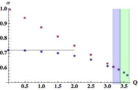

It is also possible to compare the actions for interpolating solutions with variable in a fixed total number of dimensions. In Fig. 19 we plot vs the normalized charge in for (numerical data points are shown as circles, squares, diamonds, and triangles respectively). The value of yielding an approximately zero energy dimensional vacuum in each case is denoted by the large red circle. At fixed , the solutions for always have the largest value of (and hence the highest nucleation rate). It is also of interest to compare the rates to zero energy dimensional vacua, in which case we find that the and solutions have comparable values for (because of the numerical error incurred in doing the computation it is unclear which dominates in this case). In general the comparison of nucleation rates between solutions is complicated, since there is a value of at each for which the nucleation rate is the same, and therefore vacua of different dimensionality and different cosmological constant will be populated with identical frequency. It is necessary to determine some physical criterion for making the comparison, a topic we return to in the next section.

The formation of the interpolating solution brings into being a region that relaxes to a -dimensional big crunch (when the vacuum energy is negative), or an open universe with zero or positive vacuum energy. However, when the radion potential has a positive minimum, the instantons we have found can also mediate a decompactification transition [29, 2]. The late-time -dimensional de Sitter region produced in dynamical compactification will therefore in some patches undergo transitions back to -dimensional de Sitter space. The tunneling rate out of a metastable dimensional de Sitter vacuum is given by
| (85) |
where the action of the lower dimensional de Sitter vacuum is
| (86) |
and the quantity (a ratio of actions analogous to ) is given by
| (87) |
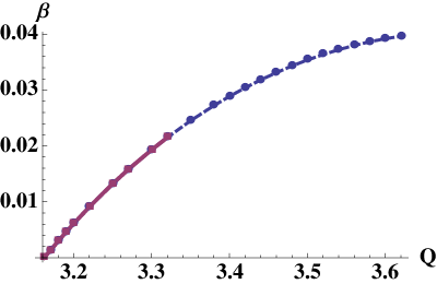
A plot of versus for is shown in Fig. 20. As , . Because the instanton action approaches a constant in this limit, , and the tunneling rate out of the -dimensional dS space is extremely suppressed, with . In the limit of a vanishing -dimensional cosmological constant, the vacuum is completely stable.
In summary,
- •
The value of at a fixed normalized charge is maximized for a particular or range of depending on the total dimensionality. If then solutions with either maximize (for ) or are comparable to solutions with (for ) or (for ). A detailed comparison of nucleation rates for vacua with different dimensionality and cosmological constant should be possible.
- •
For fixed and , the rate is highest for small , and therefore the lowest (negative) energy vacua.
- •
When it exists, the rate is higher at fixed , , and for the interpolating solution than the compactification solution. There is in general a range of for which there is a positive energy minimum, but no interpolating solution.
- •
Because the instanton action is finite as the vacuum energy of the minimum goes to zero, the rate into a -dimensional vacuum with a small (positive) vacuum energy is much higher than the rate out. -dimensional Minkowski vacua are completely stable.
VI.2 Global structure of the multiverse
Given the existence of the instantons described in the previous section, empty -dimensional de Sitter space in a theory with -form field strengths will inevitably populate all of the lower-dimensional vacua of the theory. Because the probability per unit -volume to undergo dynamical compactificaton is much smaller than a -dimensional Hubble volume , it is very rare to have more than one transition per Hubble volume per Hubble time. This implies that the -dimensional de Sitter space can never be totally eaten up by transitions and can populate many different lower-dimensional vacua, in exact analogy with four-dimensional eternal inflation. If the lower-dimensional vacua have positive vacuum energy, they are metastable, with local regions eventually transitioning back to the -dimensional de Sitter space. This recycling process continues indefinitely, fragmenting future infinity into regions with diverse properties.
When a compactification or interpolating solution is nucleated out of the -dimensional de Sitter space, it occupies nearly a Hubble volume of the background space. This can be seen by noting that both the size of the -sphere (through the location of the potential maximum Eq. 25) and the amplitude of (through Eq. 76) is set by . Thus, the naive picture that emerges is that a nucleation event corresponds to taking roughly one horizon volume of the background dS space and replacing it with the post-nucleation spacetime. In the asymptotic future, this patch then evolves into two regions: one in which the spacetime approaches a -dimensional vacuum, and the other in which it returns to the -dimensional de Sitter space.
At the very most, the region containing the -dimensional vacuum can correspond to removing a comoving Hubble volume from the background dS space. The interpolating solution is anisotropic when viewed from the full -dimensional theory, which introduces additional complications. Leaving this subtlety aside, we can course-grain, and attempt to determine how the comoving volume of the original de Sitter space is distributed between the various vacua.
Consider a fixed parcel of comoving volume that is on some fixed initial value surface everywhere in the -dimensional de Sitter space. Extending comoving geodesics from this initial value surface, we can trace the evolution as a function of proper time of the fraction of such worldlines that remain in the original vacuum to those that encounter a nucleation event of type . If we restrict our attention to the volume cut out by the nucleation events, and do not attempt to follow geodesics into the interpolating region, this should be a valid procedure. This type of volume weighting is identical to the procedures applied in various measures for eternal inflation (see for example [31], whose conventions we use below, for further discussion).
Conservation of probability implies that
| (88) |
Disregarding decompactification transitions back to the -dimensional dS space, the rate equations are
| (89) | |||||
| (90) |
where the are the probability per unit proper time to experience a transition, given by
| (91) |
The rates per unit -volume are given for the various types of transitions by Eq. 80, and is the -dimensional Hubble constant. On the initial value surface , and solving the rate equations we obtain
| (92) | |||||
| (93) |
The comoving volume fraction remaining in the -dimensional dS space goes to zero (however, the physical volume will be exponentially increasing). At late times, the distribution of worldlines reaches an equilibrium state, with the relative fraction distributed between any two vacua and given by
| (94) |
Therefore, under this measure, vacua with the largest possible values of are exponentially favored.
Taking into account the fact that there are decompactification transitions back to the -dimensional dS space requires us to follow worldlines between the vacua of different dimensionality. This will undoubtedly involve a number of important subtleties, but we might hope that a naive addition to the rate equations provides a rough picture of what happens:
| (95) | |||||
| (96) |
Here,
| (97) |
where the rates are given by Eq. 85. The full solution to the rate equations can be found using the methods outlined in [32], but considering a single transition type, the solution is
| (98) | |||||
| (99) |
Again, at late times, a steady state behavior is reached, with the relative weight of the two vacua given by
| (100) |
which is typically much greater than one, since when the scale setting the dimensional vacuum energy is much smaller than the scale setting the -dimensional vacuum energy. This result is in accord with the qualitative expectation that a statistical system spends most of its time in the state of highest entropy, and was commented on originally in Refs. [33, 2]. Here, it comes about because the rate to evolve back from the dimensional vacuum to -dimensions becomes arbitrarily small as the -dimensional vacuum energy goes to zero.
This is only one of many possible measures over the vacua produced from the background dS space. Connecting such measures to observable quantities is inherently ambiguous. For example, it is not obvious how to compare the number of observers in each unit of comoving volume, both because it is unclear what a unit of comoving volume has to do with observers, and because we are comparing infinities and there is no unique regulator (notwithstanding the fact that one must compare volumes in vacua of different effective dimensionality). We have little to add to this discussion, but it should be possible to generalize many of the existing measure proposals to this scenario. Another possibility is offered by the no-boundary proposal. Here, each Hubble volume of the background dS space is treated as an independent system, “nucleated” with probability set by the various instantons found above. The relative probability of obtaining various solutions is proportional to the ratio of rates, as in Eq. 94.
We also note that there might exist a progressive relaxation of the number of dimensions if the appropriate -form fluxes were available. In this scenario, after compactifying to , where is a -dimensional vacuum solution, a second transition could produce a product compactification . Including electric flux as well, one could consider the nucleation of charged membranes in the -dimensional vacua, embedding the standard four-dimensional picture of false-vacuum eternal inflation inside of the dynamical compactification scenario.
VII The cosmological constant problem
Within the landscape of radion potentials, it is possible to find effectively 4-dimensional vacua with positive vacuum energy. In order to promote this toy model to a plausible theory of our universe, it is necessary to ensure that there is at least one vacuum with sufficiently small positive energy to account for the observed vacuum energy [34]. This four-dimensional vacuum energy is determined by a cancellation between the curvature, flux, and higher-dimensional cosmological constant contributions to the radion potential Eq. 20. There is one vacuum per value of the charge , and since the flux should obey a quantization condition with the gauge coupling and integer, there is a discrete number of vacua.
The question of how miraculous the required cancelation is depends on how finely the vacuum energy scans with a change in the discrete values of the charge. If the gap between successive values of the vacuum energy is large, then the gauge coupling and/or higher dimensional cosmological constant would have to be extremely fine-tuned in order to produce the observed value of . However, if the gap is quite small, and there are many vacua with energies in the correct ball-park, then it is reasonable to believe that the correct vacua can be populated, even in the absence of fine-tuning.
We find two ingredients in our scenario that reduce the amount of tuning in and necessary to naturally produce the correct value of the four-dimensional cosmological constant: a large number of extra dimensions , and the presence of multiple quantized -forms with incommensurate fundamental charges. In essence, these are the same methods used by Bousso and Polchinski [35] to obtain vacua with a naturally small value of the cosmological constant, although here they arise in a different context.
If there are multiple copies of a -form, then in the radion potential Eq. 20 is replaced by the sum
| (101) |
where is the gauge coupling for each copy, and is the number of units of fundamental charge. Following Bousso and Polchinski [35], we can visualize charge space as a -dimensional grid of points with a spacing in each direction set by . Inside of this charge space, construct a shell of radius , and width . In the bulk of this shell, the total charge produces a vacuum energy between approximately zero, which defines the radius , and the observed value of the vacuum energy, which defines the width . In order for it to be likely that there is a vacuum with the appropriate value of the cosmological constant, we require that the volume contained inside of the shell is greater than the volume of a unit cell in charge space
| (102) |
where is a degeneracy in values of . If all the are different, then due to the invariance under (the total volume in the shell is reduced to the volume contained in a region with positive ). It is possible that can be somewhat larger if the are commensurate.
Applying this analysis to the radion potential, the total amount of charge necessary to produce a zero -dimensional vacuum energy can be found by substituting the approximate location of the minimum Eq. 22 into the radion potential, setting the latter to zero, and solving for . The result is an order of magnitude estimate for given by
| (103) |
For a given -dimensional vacuum energy , we can define the width by
| (104) |
where the term in parentheses is the derivative of the height of the potential minimum with respect to evaluated at . Substituting the approximate position of the potential minimum given by Eq. 22 into the radion potential and evaluating the derivative, we can find the scaling with
| (105) |
where is a function of geometrical factors only, and can be determined numerically. An example for as a function of is shown in Fig. 21, where it can be seen that this factor decreases exponentially with increasing .

Re-arranging Eq. 102, we require that
| (106) |
It is interesting and potentially significant that the effects of fine-tuning in -dimensions are amplified in the lower-dimensional theory in a number of different ways. In particular, the higher-dimensional cosmological constant is raised to a power dependent upon the number of compact dimensions and the number of fluxes, the individual gauge coupling appear as a product, and there are potentially large geometrical factors. With many compact dimensions and/or fluxes, mildly tuned values and are raised to large powers, vastly increasing the volume of the shell in charge space.
For example, taking and , the inequality is satisfied for . With more tuning in , it is possible to satisfy the inequality for smaller values of and . With , the inequality is satisfied for , , , , , or . The inequality can be satisfied for large numbers of extra dimensions or fluxes individually. For example, with , one requires and , while for , one requires for the same and . Even for the minimal values , after setting , the necessary tuning of is some orders of magnitude better than if one had started with a four-dimensional theory.
Although we will not explore the issue in detail, how finely the can lower-dimensional vacuum energy scans will also affect any potential statistical predictions of the cosmological constant. A key element in the original arguments of Weinberg [36] for an anthropic prediction of the cosmological constant is that there are many vacua inside of an “anthropic window” of acceptable vacuum energies. The validity of this assumption requires that the vacuum energy scans quite finely, and must be tested on a case-by-case basis. For example, an analysis of this issue in the context of the string theory landscape can be found in Ref. [37]. For a modern review of statistical predictions for the cosmological constant see e.g. [38, 39].
VIII Including an epoch of lower dimensional inflation
An analysis of the -dimensional cosmological constant relies on the properties of the -dimensional vacua alone. However, perhaps the most interesting feature of the solutions discussed in previous sections is the existence of a region containing a -dimensional FRW universe. The radion field dynamically evolves towards its vacuum, approaching at late times a -dimensional de Sitter, Minkowski, or big-crunch spacetime. In our universe, scalar field dynamics is thought to drive an epoch of slow-roll inflation, and it is a natural question to ask if we can embed this into our model.
We will consider two separate models of inflation in this section, both of which require the addition of a scalar field into the -dimensional theory. If this field has a positive mass squared, then it will be possible to construct the compactification, interpolating, and Nariai solutions of Sec. V exactly as before. This is not a cosmologically interesting theory, but by coupling to the -dimensional Ricci scalar and field strength, it is possible to drive the mass squared negative for large enough curvature and/or flux. In the dimensionally reduced theory, this corresponds to couplings between the radion field and the scalar , with the large curvature regime corresponding to small .
In the model shown in the left panel of Fig. 22, the instability causes to slowly-roll, while is stabilized in a minimum of the potential. In the model shown in the right panel of Fig 22, is the slowly-rolling inflaton, while is in an unstable equilibrium, eventually rolling off to a global minimum of the potential, and ending inflation. The slow-roll parameters in each case are satisfied near critical points of the potential, with slow-roll inflation occurring mostly in the direction for the potential on the left and mostly in the direction for the potential on the right.
The coupling of to curvature and flux also allows for a natural explanation of the initial conditions for inflation. For example, the potential on the left of Fig. 22 admits an interpolating solution. It is possible to adjust the couplings such that the instability in the direction develops only in the spacetime region containing the -dimensional FRW universe. In such models, slow-roll inflation in the direction is triggered by the compactification of the extra dimensions. The potential on the right of Fig. 22 does not admit an interpolating solution, but there is a compactification solution at the potential maximum along the direction. Evolution away from the maximum in the direction can drive slow-roll inflation, until the instability in the direction takes over, at which point inflation ends.

We now examine the two models of inflation in detail. In both cases, the -dimensional action we will consider is given by
| (107) |
The functions and specify the coupling to gravity and flux respectively, and has potential . The properties of the field depend on background field and metric configurations through the couplings and . It will be convenient to go to the Einstein frame in order to utilize the solutions found previously in Sec. V. After some manipulation, the action becomes
| (108) | |||||
Performing the dimensional reduction as before and going to the Einstein frame of the -dimensional theory we obtain the action
| (109) | |||||
where
| (110) |
For the moment, we will find it convenient to work with the field instead of the canonically normalized radion field .
Both models are specified by:
| (111) |
where has mass dimension and has mass dimension . Assuming an exact shift symmetry , this corresponds to the case of minimal coupling of the field to gravity and flux.
The key feature we will exploit is the -dependent mass of the field. Examining the second derivative of the potential with respect to at and fixed , we obtain
| (112) |
where . The field is stabilized at large as long as . However, if , then becomes destabilized at small . The region where becomes tachyonic allows for the possibility of an altered vacuum structure where can obtain a VEV. We assume that the second term in the potential does not affect the properties of the potential in the vicinity of , but it will be important in establishing the vacuum structure.
In order for the solutions described in Sec. V for the radion field to exist, we require in both models that the sign change in the second derivative Eq. 112 occurs somewhere between the maximum and minimum of the potential along :
| (113) |
From the discussion in Sec. II.2, if the minimum along is positive, then and . The ratio must therefore be of order for the sign change in the second derivative to occur in the desired position.
Consider first potentials of the type shown in the left panel of Fig. 22, where plays the role of the inflaton. For potentials of this type, the interpolating solution exists when the condition on the location of the second derivative Eq. 113 is satisfied. The field configuration on the big-bang surface of the -dimensional open FRW universe inside of the interpolating solution is set by the value of at the stationary point of the interpolating solution and the stabilized value . Near the minimum of , Eq. 112 becomes negative and is destabilized and begins to slowly roll.
These are essentially “hilltop” models [40]; near the minimum in , the potential is very close to quadratic over a range of of order , after which the potential steepens, and inflation ends. As is near its minimum, we can analyze this as a single-field model of inflation, where is the slowly rolling field. Inflation occurs near the maximum of the potential in the direction which this guarantees that the first slow-roll parameter
| (114) |
is small, but not the second slow-roll parameter
| (115) |
When both are small, we will find models with greater than 60 -folds of inflation. If is negligible, the spectral index is
| (116) |
Using the WMAP 5-year [34] central value of , we require . We must also ensure that the scalar power
| (117) |
is of the correct magnitude . This, together with the absence of tensor perturbations in the CMB, constrains the scale of inflation to be GeV.
Satisfying the constraint on the spectral index requires , , an to be somewhat less than one so that the second derivative Eq. 112 is sufficiently small. This represents a true tuning, and corrections will introduce the so-called “-problem” (corrections drive ). The correct scalar power can be obtained by a combination of initial conditions and either taking (scaling the entire potential) or choosing an appropriate value of such that the minimum along is of the appropriate height. One model that satisfies all of the observational constraints has the parameters . An additional tuning of is necessary in order to end inflation in a vacuum with very small cosmological constant. In this example, it is necessary to take and .
The numerical evolution of the fields in this model is shown in Fig. 23, where we have transformed from to the canonical radion field . The initial condition for the field is set by the stationary point of the interpolating solution which is approximately at . Because the field is stabilized in the -dimensional de Sitter space, it is deposited at modulo fluctuations. We might expect the size of typical fluctuations to be of order in this example. The universe begins dominated by curvature, and because the gradient in the direction is quite small, the field moves in the direction, and begins damped oscillations about the minimum in . This begins an epoch of inflation, as the field slowly rolls in the direction, as can be seen in Fig. 23. The total number of -folds depends on the initial condition for , which in this example is taken to be . This is much larger than the expected size of fluctuations, and so the total number of -folds will typically be vastly larger than the required . In fact, the potential in the direction is sufficiently flat that an epoch of slow-roll eternal inflation can be triggered inside of the interpolating solution. As long as there are enough -folds (around 60, which is not surprisingly the number typically needed to solve the flatness problem), the original curvature of the FRW region in the interpolating solution is diluted below the current bound from observations of the CMB. This is identical to the dilution required in the epoch of “open inflation” that occurs inside of bubble universes, see e.g. [41].

h
We now move to the second type of inflationary potential, shown in the right panel of Fig. 22, where plays the role of the inflaton. There is no interpolating solution for these models, and the initial conditions are set by the compactification solution. This places the field in the near-vicinity of the potential maximum in the and close to the stabilized value . If the field starts close enough to the maximum, an epoch of slow-roll eternal inflation will occur. Spacetime regions fluctuate away from the maximum, beginning slow-roll inflation with a variety of initial conditions.
This model is similar to hybrid inflation [42]; as the field slowly rolls in the direction, an instability develops in the direction that ends inflation. In these models , and an approximate inflection point develops in the direction. The scale of inflation is therefore set exclusively by the overall height of the potential, and it is necessary to take to satisfy the constraint on the scalar power. However, because we no longer need to tune the second derivative in the direction to be small, we need only ensure that becomes destabilized at an appropriate value of . This requires with and order unity. For example, a working set of parameters is . Evolution from yields the trajectory shown in Fig. 24, and produces a spectrum of fluctuations consistent with observation. Again, an additional tuning of is necessary to end inflation in a minimum with small vacuum energy. In this example, we must take and .

IX Conclusions
Despite the enormous amount of research into theories of extra dimensions, very little is known about the possible ways to make a transition from a higher-dimensional to lower-dimensional universe. In this work we have explored how such a transition might occur in one particular setting, and furthermore explored the landscape of possible vacua of different dimensions and vacuum energy that would emerge.
The starting point for this dynamical compactification scenario was -dimensional Einstein gravity in the presence of a positive cosmological constant and a set of -form field strengths. In this theory, the -dimensional de Sitter vacuum solution is semi-classically unstable to the nucleation non-singular interpolating and compactification solutions that contain a region in which of the dimensions are compact and there is a -dimensional cosmological spacetime. This region evolves towards either a big-crunch singularity or a -dimensional universe with zero or positive vacuum energy, perhaps undergoing an epoch of slow-roll inflation in the process. In this way, it is plausible that our universe arose from such a dynamical compactification of some number of extra dimensions.
The properties of the -dimensional vacua depend not only on fixed quantities such as the higher dimensional cosmological constant and total dimensionality, but also on variable quantities such as the charge and properties of other matter fields. Since the charge can take a number of values, and there can be multiple kinds of flux, a landscape of vacua with different vacuum energy and effective dimensionality emerges. Each of these vacua is populated by the dynamical compactification process described above. This mechanism of landscape population is fundamentally different from false vacuum eternal inflation, which operates entirely within the realm of the lower-dimensional effective theory. 44 4 In the landscape of Type IIB string theory, the volume modulus can provide an obstacle to populating vacua through eternal inflation [43], and it is interesting to identify an alternative mechanism. Since the interpolating solutions are close cousins of non-extremal -branes, their semi-classical production is more analogous to the nucleation of charged black holes in de Sitter space.
In any theory where a number of vacua are realized in different spatiotemporal regions, the prediction of the parameters in a low-energy effective theory becomes statistical at best. Such a prediction will necessarily involve both dynamics and selection effects. Before tackling such complicated questions, a zeroth order requirement is for the theory to contain at least one vacuum with the observed properties of our universe. In our toy model, we can ask if there are vacua with the correct dimensionality and the observed value of the cosmological constant. Finding vacua of the correct dimensionality requires that there exists a -form field strength. Naturally obtaining the observed value of the cosmological constant requires that there is 1) tuning of the higher dimensional cosmological constant, 2) tuning of the fundamental unit of charge associated with the flux, 3) multiple types of -form flux with incommensurate charges, 4) many extra dimensions, or some combination thereof. This is very similar to the story in the string theory landscape.
To gain some understanding of the dynamics, we have explored the phenomenology of nucleation rates. Generically, the rates are suppressed by some appreciable fraction of the higher dimensional de Sitter action, and are higher for smaller values of the lower dimensional vacuum energy (the highest rate is to the most negative minimum). Another interesting behavior arises when comparing the rate to vacua of different dimensionality, which at fixed normalized charge is maximized for a particular or range of depending on the total dimensionality. Comparing the rate into a -dimensional vacuum to the rate for decompactification back to -dimensions, we find in agreement with previous studies that Minkowski vacua are completely stable and the rate into a -dimensional vacuum with a small positive vacuum energy is much higher than the rate out. These rates can be used to examine the structure of the higher-dimensional multiverse, for example calculating the distribution of comoving volume.
Although we have presented a relatively complete picture of the solutions and their nucleation, we have neglected a number of potentially important effects. Perhaps the most pressing is the question of stability. It is well known that black branes in flat space are unstable [44], which may have implications for the stability of the interpolating solutions. The stability of the compactification solutions was examined in Ref. [33] (see also [45, 46]), where an instability was discovered for . This is perhaps troubling since the existence of more than 3 extra dimensions is theoretically well motivated from string theory.
Recently this problem was revisited in Ref. [47], who found stable warped solutions for , and proposed that such solutions are the endpoint of evolution from the unstable solutions without warping. In this case, the existence of an instability would not affect the qualitative aspects of our analysis in any number of dimensions, but addressing this question in more detail is clearly necessary.
In addition, there are many are many directions in which one could proceed to make more detailed and quantitative predictions in this multiverse model. This necessarily involves determining an appropriate measure over the various solutions, but there may be other more direct signatures. For example, in false vacuum eternal inflation, it is known that the inevitable collisions between bubble universes might lead to direct signatures of other bubble universes [48]. In complete analogy, we might expect that some of the interpolating solutions overlap, leading to potentially observable inhomogeneities in the -dimensional cosmologies. This situation is also analogous to multi-centered black hole and black brane solutions.
It is hoped that this model will provide different insights into issues surrounding extra dimensions and theories with multiple vacua than those obtained by studying eternal inflation in the string theory landscape.
Acknowledgements.
The authors wish to thank Rob Myers and Matt Kleban for helpful conversations. Partial support for this research was provided by the U.S. Department of Energy and the Gordon and Betty Moore Foundation. L.R. thanks the California Institute of Technology, the Moore Fellowship Program, and NYU for their hospitality while this work was completed. L.R. is supported by NSF grant PHY-0556111.Appendix A Homogenous but anisotropic solutions
A more general -dimensional metric ansatz is to assume homogeneity but not isotropy. In four dimensions, these are the Bianchi-type cosmologies. Here, we detail the construction of solutions without spatial curvature, although it is possible to generalize our methods to all homogenous solutions in any number of dimensions. For flat spatial sections, the most general homogenous metric can be written as
| (118) |
where the are cartesian coordinates that generally range between . There are (dimensionless) scale factors which are all arbitrary functions of .
It is possible to decouple the Einstein equations by finding equations of motion for the field and the product of metric functions
| (119) |
Making this substitution yields
| (120) |
| (121) |
| (122) |
The constant parametrizes the degree of anisotropy, and is related to the metric functions as we outline below.
The Ricci scalar is again given by Eq. 39 (as can be explicitly checked using the equations of motion), and so as long as the field and its derivatives remain finite, the surface is completely non-singular. From the field equation Eq. 122, this requires that . The surfaces correspond to event horizons in the -dimensional geometry, just as they did in the black hole example of the Introduction. From Eq. 120, if the field and its derivatives stay finite, then the anisotropy term always dominates at small . This leads to the universal behavior as , which can be recognized as the Kasner solution.
The value of and the time dependence of the individual can be found from the remaining Einstein equations. Near , the metric is always in the form of the Kasner solution, where the scale factors are a power law in
| (123) |
There are two Kasner conditions
| (124) |
that constrain the exponents . It can be shown that unless there is a single non-zero , at least one of the must be negative (see e.g. Ref. [49]). This implies that if there is more than one non-zero , at least one scale factor diverges at , while the others shrink to zero. If it is possible to continue across the surface to a region where is spacelike, only one of the metric functions can go to zero (otherwise the analytic continuation becomes ambiguous). Therefore, in the vicinity of , only one of the Kasner exponents can be positive. From the Kasner conditions, in order to obtain with a single positive Kasner exponent, all of the other exponents must be zero.
From the equations of motion, the anisotropy parameter is given by
| (125) |
The full time dependence of the scale factors can be determined by identifying a number of constants of the motion. For example, specializing to , and following Ref. [50], there are three constants of the motion
| (126) |
One then obtains equations for and
| (127) | |||||
| (128) |
The anisotropy parameter is given in terms of the constants of motion by
| (129) |
The time-dependence of can then be determined from . This procedure can be applied in an arbitrary number of dimensions by again identifying the appropriate constants of the motion.
A.1
We now construct anisotropic solutions in the absence of a -dimensional cosmological constant. Before analyzing the dimensionally reduced theory, we briefly discuss some analytic solutions that can be generated from an anisotropic metric ansatz. Included in this set of solutions are the extremal and non-extremal -brane solutions of Ref. [51]. The metric for such solutions in D-dimensions is given by [15]
| (130) | |||||
where and are the two event horizons related to the charge by
| (131) |
There is a curvature singularity at . When , the event horizons become degenerate, and the solution is said to be extremal. These are none other than the extremal solutions we constructed in Sec. IV. It is also possible to have super-extremal solutions, in which there is a naked singularity (these are similar to the timelike singular solutions of Sec. IV).
In the region between the horizons , is a timelike variable. Near the horizon at , we now show that the metric is of the Kasner form. This can be done analytically for by dimensionally reducing to 4-dimensions and performing a conformal transformation to the 4-dimensional Einstein frame. The metric Eq. 130 becomes
| (132) | |||||
Changing coordinates to
| (133) |
and expanding to lowest order around the horizon at
| (134) | |||||
Re-scaling , , and by the constant factors, we obtain
| (135) |
Finally, defining the proper time variable , we recover the metric
| (136) |
This is of the Kasner form, with all but one of the exponents zero as expected.
The non-extremal -brane solutions discussed above can also be obtained from the dimensionally reduced theory by evolving in the presence of the radion potential, just as in the analysis of Sections III, IV, and V. The non-extremal, extremal, and super-extremal -brane solutions correspond to different initial conditions for the radion field. In fact, these are the only solutions that possess an asymptotically flat -dimensional region, and the radion and scale factor profiles will be qualitatively similar to the extremal and singular (timelike and spacelike) solutions found in Sec. IV.
Our method of constructing solutions in the dimensionally reduced theory will be identical to the procedure outlined in Sec. III, where spacetime regions with timelike and spacelike are matched across event horizons. We will discuss the evolution of the radion field in each case separately.
Returning to the equations of motion for , it can be seen from Eq. 121 that the sign of the second time derivative of is fixed by the sign of . For , the potential for is negative in the vicinity of the potential minimum and approaches zero from below as . Evolution to is therefore in a spacetime region where is a spacelike variable and . Just as for the maximally symmetric case, there are attractor solutions approached from generic initial conditions. The analysis is similar to that of Sec. III.
We now look for solutions in regions where is a timelike variable as in Eq. 118. Concentrating on motion in the vicinity of the potential minimum, we can apply the methods used in Sec. III. Since the minimum is negative, the scale factor is bounded, with the frequency of motion given from Eq. 121 by
| (137) |
Substituting into the field equation Eq. 122, the solutions for can be written in terms of Gegenbauer polynomials, with the index determined by
| (138) |
which, substituting with Eq. 58, yields independent of . Therefore, for solutions with stationary points infinitely close to the minimum, there are solutions that interpolate across the minimum exactly once, and the oscillatory solutions found in Sec. V cannot not exist. For an initial condition displaced slightly from the minimum, the frequency increases, causing the solutions to go singular in the vicinity of the would-be second stationary point.
Putting the full solution together, if there is a non-singular stationary point on the right side of the potential minimum, then it is possible to connect the asymptotic region with spacelike across an event horizon to a region in the basin of attraction of the minimum with timelike that contains a singularity. This is exactly the expected behavior for the non-extremal -branes discussed previously. The causal structure will resemble the singular (spacelike) solutions of Sec. V. If there is no non-singular stationary point, then the geometry will contain a timelike naked singularity. The causal structure in this case will be identical to the singular (timelike) solution described in Sec. V. The extremal solution will be identical to the solution obtained in Sec. IV, since the regime where the anisotropy dominates the energy density is pushed to .
A.2
When , the potential approaches zero from above, implying that is a timelike variable in the asymptotically -dimensional region of the geometry. There are attractor solutions where is timelike interpolating between a non-singular stationary point and of the type discussed in Sec. V. Continuing across the stationary point to a region where is spacelike, we can look for motion in the vicinity of the inverted potential maximum. The solution for the scale factor is oscillatory and the solution for the field is again a Gegenbauer polynomial with index given by the solution to
| (139) |
The solution for is always less than one, implying that there are no non-singular trajectories crossing the maximum of the potential – the field cannot evolve quickly enough to traverse the maximum before the scale factor hits its second zero. Thus, in contrast to the solutions in Sec. IV for an FRW metric ansatz, there can be no interpolating solutions connecting the asymptotic region to the potential minimum. The geometries will therefore have a causal structure similar to the singular solutions of Sec. IV. Moving the stationary point in the motion of the radion field to the potential maximum, the anisotropy becomes unimportant, and it will be possible to find the Nariai solution discussed in Sec. IV
References
- [1] L. Susskind (2003), eprint hep-th/0302219.
- [2] S. B. Giddings and R. C. Myers, Phys. Rev. D70, 046005 (2004), eprint hep-th/0404220.
- [3] R. H. Brandenberger and C. Vafa, Nucl. Phys. B316, 391 (1989).
- [4] A. Karch and L. Randall, Phys. Rev. Lett. 95, 161601 (2005), eprint hep-th/0506053.
- [5] F. Larsen and F. Wilczek, Phys. Rev. D55, 4591 (1997), eprint hep-th/9610252.
- [6] S. M. Carroll, M. C. Johnson, and L. Randall (2009), eprint 0901.0931.
- [7] R. Bousso and S. W. Hawking, Phys. Rev. D52, 5659 (1995), eprint gr-qc/9506047.
- [8] R. Bousso and S. W. Hawking, Phys. Rev. D54, 6312 (1996), eprint gr-qc/9606052.
- [9] R. Bousso, Phys. Rev. D55, 3614 (1997), eprint gr-qc/9608053.
- [10] R. Bousso and S. W. Hawking, Int. J. Theor. Phys. 38, 1227 (1999).
- [11] S. W. Hawking and S. F. Ross, Phys. Rev. D52, 5865 (1995), eprint hep-th/9504019.
- [12] R. B. Mann and S. F. Ross, Phys. Rev. D52, 2254 (1995), eprint gr-qc/9504015.
- [13] P. H. Ginsparg and M. J. Perry, Nucl. Phys. B222, 245 (1983).
- [14] R. Bousso, Phys. Rev. D60, 063503 (1999), eprint hep-th/9902183.
- [15] G. W. Gibbons, G. T. Horowitz, and P. K. Townsend, Class. Quant. Grav. 12, 297 (1995), eprint hep-th/9410073.
- [16] G. W. Gibbons and D. L. Wiltshire, Nucl. Phys. B287, 717 (1987), eprint hep-th/0109093.
- [17] H. Lu, S. Mukherji, and C. N. Pope, Int. J. Mod. Phys. A14, 4121 (1999), eprint hep-th/9612224.
- [18] K. Behrndt and S. Forste, Nucl. Phys. B430, 441 (1994), eprint hep-th/9403179.
- [19] E. A. Bergshoeff, A. Collinucci, D. Roest, J. G. Russo, and P. K. Townsend, Class. Quant. Grav. 22, 4763 (2005), eprint hep-th/0507143.
- [20] C. Krishnan, S. Paban, and M. Zanic, JHEP 05, 045 (2005), eprint hep-th/0503025.
- [21] P. G. O. Freund and M. A. Rubin, Phys. Lett. B97, 233 (1980).
- [22] J. J. Halliwell, Phys. Lett. B185, 341 (1987).
- [23] B. Ratra and P. J. E. Peebles, Phys. Rev. D37, 3406 (1988).
- [24] A. R. Liddle, Phys. Lett. B220, 502 (1989).
- [25] S. R. Coleman, Phys. Rev. D15, 2929 (1977).
- [26] L. F. Abbott and S. R. Coleman, Nucl. Phys. B259, 170 (1985).
- [27] S. W. Hawking and I. G. Moss, Phys. Lett. B110, 35 (1982).
- [28] P. Batra and M. Kleban, Phys. Rev. D76, 103510 (2007), eprint hep-th/0612083.
- [29] S. B. Giddings, Phys. Rev. D68, 026006 (2003), eprint hep-th/0303031.
- [30] S. R. Coleman and F. De Luccia, Phys. Rev. D21, 3305 (1980).
- [31] J. Garriga and A. Vilenkin, Phys. Rev. D57, 2230 (1998), eprint astro-ph/9707292.
- [32] S. Winitzki, Lect. Notes Phys. 738, 157 (2008), eprint gr-qc/0612164.
- [33] R. Bousso, O. DeWolfe, and R. C. Myers, Found. Phys. 33, 297 (2003), eprint hep-th/0205080.
- [34] E. Komatsu et al. (WMAP), Astrophys. J. Suppl. 180, 330 (2009), eprint 0803.0547.
- [35] R. Bousso and J. Polchinski, JHEP 06, 006 (2000), eprint hep-th/0004134.
- [36] S. Weinberg, Phys. Rev. Lett. 59, 2607 (1987).
- [37] D. Schwartz-Perlov and A. Vilenkin, JCAP 0606, 010 (2006), eprint hep-th/0601162.
- [38] A. Vilenkin (2004), eprint astro-ph/0407586.
- [39] R. Bousso, Gen. Rel. Grav. 40, 607 (2008), eprint 0708.4231.
- [40] L. Boubekeur and D. H. Lyth, JCAP 0507, 010 (2005), eprint hep-ph/0502047.
- [41] B. Freivogel, M. Kleban, M. Rodriguez Martinez, and L. Susskind, JHEP 03, 039 (2006), eprint hep-th/0505232.
- [42] A. D. Linde, Phys. Lett. B259, 38 (1991).
- [43] M. C. Johnson and M. Larfors, Phys. Rev. D78, 123513 (2008), eprint 0809.2604.
- [44] R. Gregory and R. Laflamme, Phys. Rev. Lett. 70, 2837 (1993), eprint hep-th/9301052.
- [45] O. DeWolfe, D. Z. Freedman, S. S. Gubser, G. T. Horowitz, and I. Mitra, Phys. Rev. D65, 064033 (2002), eprint hep-th/0105047.
- [46] C. R. Contaldi, L. Kofman, and M. Peloso, JCAP 0408, 007 (2004), eprint hep-th/0403270.
- [47] S. Kinoshita and S. Mukohyama (2009), eprint 0903.4782.
- [48] A. Aguirre, M. C. Johnson, and A. Shomer, Phys. Rev. D76, 063509 (2007), eprint 0704.3473.
- [49] C. W. Misner, K. S. Thorne, and J. A. Wheeler, Gravitation (Freeman, San Francisco, 1973).
- [50] M. Demianski, R. de Ritis, C. Rubano, and P. Scudellaro, Phys. Rev. D46, 1391 (1992).
- [51] G. T. Horowitz and A. Strominger, Nucl. Phys. B360, 197 (1991).