Improving PSF modelling for weak gravitational lensing using new methods in model selection

The starting point in this analysis is to construct a simplified description of the process of modelling PSF anisotropy across the $x$-$y$ plane, such as across a telescope field of view. In what follows the discussion is limited to models of complex, spin-2 pseudo-vector fields (i.e. $f(x,y)=|f|(x,y)\mbox{$\mathrm{e}$}^{\mbox{\scriptsize$\mathrm{i}$}2\theta(x,y)}$) on a 2D plane, but such arguments may be generalized to scalar or spin-$n$ fields, and to other spatial dimensionalities (see Section 8).

An observed complex ellipticity field is described as the sum of two contributions, the unknown ‘true’ ellipticity field $e_{\mbox{\scriptsize$\mathrm{t}$}}$ and $N$, a stochastic complex variable describing noise upon ellipticity measurements. This field is labelled $e(x,y)=e_{1}+\mbox{$\mathrm{i}$}e_{2}$, where:

In almost all that follows the explicit $x$-$y$ dependence of fields such as $e_{\mbox{\scriptsize$\mathrm{t}$}}$ will be dropped for brevity, and should be implied. The description of discrete observations $e_{i}$ by a continuous ‘quasi-field’ $e$ is also a notational convenience: measured quantities will always be an $e(x_{i},y_{i})$ sample of the proposed field $e$. We assume that the stochastic noise term satisfies $\left\langle N\right\rangle=0$.

If a best fit parametrized model is then applied to describe $e$, one can choose to write the modelled ellipticity $e_{\mbox{\scriptsize$\mathrm{m}$}}$ as

where $m=e-e_{\mbox{\scriptsize$\mathrm{t}$}}$ will hereafter be referred to as the inaccuracy in the model, also unknown, and $f_{\mbox{\scriptsize$\mathrm{m}$}}$ is simply a label denoting the functional scheme used to fit the spatial variation of $e$ (e.g. a second order bivariate polynomial). This expression makes explicit the dependence of the inaccuracy $m$ upon $e_{\mbox{\scriptsize$\mathrm{t}$}}$, the ensemble of discrete realizations of $N$, and $f_{\mbox{\scriptsize$\mathrm{m}$}}$. In general this dependence will be non-trivial to describe, but the aim of this paper is to look for diagnostic tests by which the functional properties of $m$ can be constrained.

The principal tool in this work is the two point ellipticity correlation function, the observable quantity used to extract signal in cosmic shear studies. In this the investigation follows Hoekstra (2004), as well as the later work of Van Waerbeke et al. (2005) and Hoekstra et al. (2006), in analyzing correlations in corrected PSF patterns as a means of testing anisotropy models. Specifically the $\xi_{\pm}(r)$ correlation functions will be used, defined as

where $e_{\mbox{\scriptsize$\mathrm{tan}$}}$ and $e_{\times}$ are the known as the tangential and rotated components of the ellipticity, and the angle brackets denote an averaging over all pairs of points separated by a distance $r$. It should be noted therefore that this definition implicitly averages over all angles, which is not a problem in the cosmic shear case where correlations are assumed isotropic so that $\xi(\mbox{\boldmath$r$})=\xi(r)$; if the field is not strictly isotropic then it must be borne in mind that $\xi(r)$ is the angular average correlation, and thus that some information may have been lost.

The tangential and rotated components are defined for the complex ellipticities $e$ of each pair as

(see, e.g., Schneider, 2006), where $\phi$ is the angle between the abscissa and the line joining the location of each member of the pair of points. With a discrete number of ellipticity measurements the quantities in equation (3) can then be estimated by

in finite bins of $r$. Such correlation function estimates, when made using PSF-corrected galaxy ellipticities, are the primary observable quantity in modern studies of cosmological weak lensing (see, e.g., Fu et al., 2008; Schrabback et al., 2007).

In the following discussion, which focuses upon $\xi_{+}$ as a diagnostic of PSF modelling, frequent use will be made of a useful shorthand notation:

Due to parity symmetry (see Schneider, 2006) the imaginary second term in equation (7) tends to zero, and so $\left\langle e^{*}e\right\rangle(r)=\xi_{+}(r)$. Similarly, $\left\langle e^{*}_{\mbox{\scriptsize$\mathrm{m}$}}e_{\mbox{\scriptsize$\mathrm{m}$}}\right\rangle(r)$ will be used to denote the $\xi_{+}(r)$ autocorrelation in the model $e_{\mbox{\scriptsize$\mathrm{m}$}}$. This notation is convenient not only as a labelling convention but also as a computational tool, and so will be used exclusively hereafter.

In order to proceed, two simplifying assumptions are made about the noise. Firstly, it is assumed that $N$ is spatially uncorrelated so that

for all $r>0$. Secondly, it is assumed that the cross-correlation between $N$ and the unknown $e_{\mbox{\scriptsize$\mathrm{t}$}}$ is also zero, so that

Situations in which equations (8) and (9) no longer hold can be envisaged, such as in the presence of problems with reduced Charge Transfer Efficiency (CTE) in telescope CCDs (see, e.g.  Rhodes et al., 2007) or preferences for certain PSF directions due to large pixel sizes or under sampled stellar images. In this theoretical analysis these factors are assumed to be small, but if necessary the assumption may be easily tested and corrected for using simulated data.

For an ideal fit $m=0$ everywhere, but this is unrealistic in the case of noisy data and finite numbers of observations. For the case of an imperfect but well-constrained, stable and accurately predictive model the following three conditions should be simultaneously fulfilled:

for all $r>0$. These conditions will be met if the modelling inaccuracies $m$ can, like the noise, be approximately described as an independent, stochastic variable $m=M$ with $\left\langle M\right\rangle=0$.

The first of these conditions (10) requires that the inaccuracies $m$ should be distributed at random with respect to the true ellipticity distribution, and thus that the cross-correlation between these quantities be zero; this condition will be broken if the model is systematically underfitting the true ellipticities $e_{\mbox{\scriptsize$\mathrm{t}$}}$, as will be discussed in Section 2.3 below. The second condition (11) explicitly states that $m$ is required to be uncorrelated with the noise $N$, expected if the scheme $f_{\mbox{\scriptsize$\mathrm{m}$}}$ allows significant overfitting of the data. The third and final condition (12) requires that $m$ show no spatial autocorrelation, which will be fulfilled if the inaccuracies at all points are mutually randomly distributed. This third condition may be broken for both overfitting, where neighbouring $m$ values may be correlated to the extent allowed by instabilities in the chosen $f_{\mbox{\scriptsize$\mathrm{m}$}}$, and underfitting, where $e_{\mbox{\scriptsize$\mathrm{m}$}}$ systematically fails to reproduce observable features in $e_{\mbox{\scriptsize$\mathrm{t}$}}$.

Unfortunately, the functions in equations (10)-(12) cannot be measured directly, as $m$, $N$ and $e_{\mbox{\scriptsize$\mathrm{t}$}}$ are unknown. However, it is possible to construct two independent, observable correlation functions with which to attempt to constrain these quantities. There is freedom in how these are defined (as will be discussed below), but the following useful forms are suggested:

These two diagnostic quantities $D_{1}$ and $D_{2}$ may be easily estimated from modelled stellar fields using routines that are standard in statistical lensing. Using the definitions and assumptions described by equations (1)-(9), they can be expressed in terms of the unknown quantities as follows:

It is noted immediately that there are only two quantities with which to constrain the three unknowns of conditions (10)-(12), and the system is therefore underdetermined. This is a natural consequence of there being only two directly observable quantities ($e$ and $e_{\mbox{\scriptsize$\mathrm{m}$}}$) with which to place constraints upon correlations in $m$, $N$ and $e_{\mbox{\scriptsize$\mathrm{t}$}}$. The system of equations described by (15) and (16) cannot therefore be solved to demonstrate any of (10)-(12) uniquely. Instead, one may determine only a general family of solutions. In vector notation this solution is simply

where $t$ is any real number. Attempts to construct a third independent observable with which to break this degeneracy do not succeed: for example, the observable function $\left\langle e^{*}e\right\rangle-\left\langle e^{*}_{\mbox{\scriptsize$\mathrm{m}$}}e_{\mbox{\scriptsize$\mathrm{m}$}}\right\rangle$ may be written simply as $D_{2}-D_{1}$.

The fact that this system of equations is underdetermined means the $D_{1}(r)$ or $D_{2}(r)$ diagnostics can never be used to prove that $\left\langle m^{*}m\right\rangle=\left\langle m^{*}N+N^{*}m\right\rangle=\left\langle m^{*}e_{\mbox{\scriptsize$\mathrm{t}$}}+e^{*}_{\mbox{\scriptsize$\mathrm{t}$}}m\right\rangle=0$ at all scales. However, they allow the positive diagnosis of poor modelling if either are nonzero at a significant level. Moreover, in order to be erroneously led into the belief that a given model fit is accurate and stable would require that

for all scales $r$, constituting a significant coincidence and very poor luck. Finally, although the general expression in (17) allows an infinite family of solutions to our three quantities (10-12), this solution is not the only information we have. Further assumptions and simple reasoning may be employed so as to predict what might be expected for these diagnostic measures in the cases of over- or underfitting; this in turn may allow the tuning of modelling schemes so as to better represent the data without fitting noise. These reasoned expectations for the general form of $D_{1}(r)$ and $D_{2}(r)$ will now be outlined.

In order to describe what might be expected in the case of underfitting, we consider a hypothetical scheme $f_{\mbox{\scriptsize$\mathrm{m}$}}$ for which the model ellipticities $e_{\mbox{\scriptsize$\mathrm{m}$}}$ do not adequately represent the underlying field $e_{\mbox{\scriptsize$\mathrm{t}$}}$. This can be expressed in terms of the simple model constructed in Section 2.1, and the further assumption that in the limit of severe underfitting it may be approximated that

The validity of this approximation will depend strongly upon the degree to which a given fit fails to reproduce observable features in $e_{\mbox{\scriptsize$\mathrm{t}$}}$, but it can be motivated by an illustrative example: a flat model scheme $f_{\mbox{\scriptsize$\mathrm{m}$}}$ for which $e_{\mbox{\scriptsize$\mathrm{m}$}}=\left\langle e\right\rangle=$ constant being used to describe an $e_{\mbox{\scriptsize$\mathrm{t}$}}$ which varies significantly with $x$ and $y$. In this case $m=\left\langle e\right\rangle-e_{\mbox{\scriptsize$\mathrm{t}$}}$, which is a clear function of $e_{\mbox{\scriptsize$\mathrm{t}$}}$ and only very weakly dependent upon the noise via $\left\langle e\right\rangle$.

Given the assumption of equation (19), it should be expected that $m$ is approximately uncorrelated with the noise $N$ for underfitting models (carrying only a weak dependence upon it), and thus that

The condition expressed in equation (11) is therefore approximately fulfilled for underfitting models, meaning that observations of $D_{1}(r)$ and $D_{2}(r)$ will provide constraints upon the quantities in equations (10) and (12). Using equations (13) and (14), this then gives

These predictions can now be used to make further conclusions as to the expected form of these functions, allowing the positive diagnosis of underfitting models if these expected forms are observed.

From equation (19) it is clear that the form taken by $\left\langle m^{*}m\right\rangle$ will be related to that of $\left\langle e^{*}_{\mbox{\scriptsize$\mathrm{t}$}}e_{\mbox{\scriptsize$\mathrm{t}$}}\right\rangle$, and if the underfitting is significant then $\left\langle m^{*}m\right\rangle$ is likely to be nonzero on or near the scales for which $\left\langle e^{*}_{\mbox{\scriptsize$\mathrm{t}$}}e_{\mbox{\scriptsize$\mathrm{t}$}}\right\rangle$ is nonzero. Figure 1 shows a simple example of how both correlation and anticorrelation might be expected in underfitting model residuals; in this simple example of a one-dimensional underfitting model the residuals within the cross-containing regions will be positively correlated, but between these regions the residuals will be negatively correlated. Turning to the simple $e_{\mbox{\scriptsize$\mathrm{m}$}}=\left\langle e\right\rangle$ model for another illustration, using equations (22) and $\left\langle N\right\rangle\simeq 0$ it may be written that $D_{1}(r)\simeq\left\langle e_{\mbox{\scriptsize$\mathrm{t}$}}^{*}e_{\mbox{\scriptsize$\mathrm{t}$}}\right\rangle-\left|\left\langle e_{\mbox{\scriptsize$\mathrm{t}$}}\right\rangle\right|^{2}$. Therefore, this $D_{1}(r)$ may potentially be both positive or negative for differing ranges $r$, depending upon the functional form of $e_{\mbox{\scriptsize$\mathrm{t}$}}$.

This behaviour will also be expected from the second measurable quantity $D_{2}(r)$, which from equation (23) will also be activated by underfitting: $\left\langle m^{*}e_{\mbox{\scriptsize$\mathrm{t}$}}+e^{*}_{\mbox{\scriptsize$\mathrm{t}$}}m\right\rangle$ will often be nonzero for $m\simeq m(e_{\mbox{\scriptsize$\mathrm{t}$}};f_{\mbox{\scriptsize$\mathrm{m}$}})$. The function $D_{2}(r)$ may be rewritten by considering that $m=e_{\mbox{\scriptsize$\mathrm{m}$}}-e_{\mbox{\scriptsize$\mathrm{t}$}}$, giving

Once again, $D_{2}(r)$ may be expected to be either positive or negative depending upon scale $r$ and the sign of $\left\langle e^{*}_{\mbox{\scriptsize$\mathrm{t}$}}e_{\mbox{\scriptsize$\mathrm{t}$}}\right\rangle$. However, the precise dependence of $D_{2}(r)$ may differ from that of $D_{1}(r)$ in a way that is difficult to predict without detailed knowledge of the $e_{\mbox{\scriptsize$\mathrm{t}$}}$ field.

The case of overfitting is now considered so as to make predictions for the behaviour of $D_{1}(r)$ and $D_{2}(r)$: if the behaviour differs from the underfitting case this will allow the two cases to be distinguished and positively identified, and allow subsequent modelling improvements to be made in a guided fashion. As mentioned in Section 1, the application of PCA to PSF modelling (Jarvis & Jain, 2004) also brings control over overfitting via the removal of identified low-importance principal components. However, it may be that a hybrid of PCA and the simultaneous fitting of an independent surface is necessary to account for random changes in the PSF pattern between exposures, and so a diagnosis of possible overfitting in this extra surface will still be desirable. Moreover, the behaviour of $D_{1}(r)$ and $D_{2}(r)$ in overfitting models is an interesting investigation in itself, as the technique may be useful in other situations in which PCA is not directly applicable (see Section 7).

In Section 2.3 the inaccuracy $m$ was approximated as being a function of $e_{\mbox{\scriptsize$\mathrm{t}$}}$ and $f_{\mbox{\scriptsize$\mathrm{m}$}}$ only. A similar approximation can be argued for the opposing case of severe overfitting:

This statement can be justified by considering what is meant by an overfitting model: one which captures not only an observable physical trend, but is also unjustifiably sensitive to random noise upon measurements. Such models will not in general be biased in a way that can be related to $e_{\mbox{\scriptsize$\mathrm{t}$}}$, but will prove to be unstable with respect to changes in $N$ (this concept is also discussed in Paulin-Henriksson et al., 2009). The correlation properties of $m$ are now largely decided by this random quantity and inherent correlations caused by the best-fitting chosen model $f_{\mbox{\scriptsize$\mathrm{m}$}}$. Taking this assumption, and using equations (25) and (9), leads to

via the same reasoning as equation (20). This corresponds to saying that condition (10) will be fulfilled when severely overfitting data, just as in Section 2.3 it was argued that condition (11) is automatically fulfilled if data is being underfit.

Using this result, the effects of overfitting upon the forms of $D_{1}(r)$ and $D_{2}(r)$ can be predicted. From equations (13), (14), and (27) it may be written that

It is noted immediately that the expression for $D_{1}(r)$ remains unsimplified: unlike $\left\langle m^{*}e_{\mbox{\scriptsize$\mathrm{t}$}}+e^{*}_{\mbox{\scriptsize$\mathrm{t}$}}m\right\rangle$, the $\left\langle m^{*}m\right\rangle$ term will not necessarily vanish for overfitting models, despite the assumption of uncorrelated noise in equation (8). As can be seen from equation (25), there remains the possibility of correlation due to the inherent properties of the functional form of the model $f_{\mbox{\scriptsize$\mathrm{m}$}}$ used to unstably fit the data.

It is expected that the condition (12) is not fulfilled when we are overfitting the data, and thus that $D_{2}(r)$ will be nonzero. It can furthermore be said that a positive cross-correlation will be expected between $N$ and $m$, so that

This can be justified by considering once again $m=e_{\mbox{\scriptsize$\mathrm{m}$}}-e_{\mbox{\scriptsize$\mathrm{t}$}}$, which combined with equation (9) then gives

This last inequality indeed expresses a definition of overfitting, being that the best-fitting model $e_{\mbox{\scriptsize$\mathrm{m}$}}$ shows some significant average correlation with the particular realization of the noise $N$. It is then clear from equations (29) and (31) that

i.e. nowhere positive and potentially significantly negative, for overfitting models. In Section 2.3 it was seen that $D_{2}(r)$ is expected to be positive over some range of $r$ for severely underfitting models. Whilst the minimization of $D_{2}(r)$ will lead to an optimal fit in any case, this difference in behaviour between under- and overfitting offers hope of diagnosing successfully between the two cases, allowing informed improvements in modelling to be made at each stage.

Furthermore, it can be argued that in most cases the $\left\langle m^{*}m\right\rangle$ due to undue freedom in the model $f_{\mbox{\scriptsize$\mathrm{m}$}}$ will be small compared to $\left\langle m^{*}N+N^{*}m\right\rangle$; if this is so the $D_{1}(r)$ function may also be used to distinguish under- and overfitting. The argument relies on the following insight: an overfitting model, but one that has nevertheless been constructed by minimizing deviations from the observed data, will in all but the most pathological cases be expected to have inaccuracies $|m(N;f_{\mbox{\scriptsize$\mathrm{m}$}})|\leq|N_{i}|$ at each point $(x_{i},y_{i})$. The limiting example of this behaviour is an ‘ultimate overfit’, for which the model is simply $e_{\mbox{\scriptsize$\mathrm{m}$}}=e$ (and thus $m=N$), with an interpolation or spline between stellar data points. Such a model takes no account of the fact that there may be noisy or imperfect measurements among the input data. Using $|m(N;f_{\mbox{\scriptsize$\mathrm{m}$}})|\leq|N|$ then gives

which in turn implies that

in the same way as $D_{2}(r)$. This offers further hope of positive, distinguishable diagnoses of both under- and overfitting, based on whether $D_{1}(r)$ and $D_{2}(r)$ are observed to be both positive and negative, or negative only, respectively.

To summarize, the functional behaviour of the $D_{1}(r)$ and $D_{2}(r)$ diagnostic functions for both over- and underfitting modelling schemes $f_{\mbox{\scriptsize$\mathrm{m}$}}$ has been predicted using simple assumptions about the nature of the modelling, the noise, and the data themselves. The most important, and potentially least secure, of these assumptions are the validity of the approximate functional dependencies of $m$, given in equations (19) and (25). In order to test these points of reasoning, and to explore the strength of each diagnostic function in a realistic modelling situation, the following Section will test the efficacy of $D_{1}(r)$ and $D_{2}(r)$ using a simulated PSF anisotropy map with a known, underlying ellipticity model.

The simulated starfield is designed to mimic measurements of ellipticity from 2500 stars across a square telescope field of view of area 1 deg². The number of stars in the field, the field shape, typical PSF anisotropy and measurement noise are loosely based upon lensing observations from the Canada-France-Hawaii Telescope Legacy Survey-Wide (CFHTLS-W, e.g. Fu et al., 2008; Hoekstra et al., 2006). An ellipticity measurement $e$ was assigned to each star as modelled in equation (1), consisting of a true underlying model $e_{\mbox{\scriptsize$\mathrm{t}$}}$ and additive noise term $N$, each scaled so as to resemble the CFHTLS-W.

In order to construct $e_{\mbox{\scriptsize$\mathrm{t}$}}(x,y)$ the telescope field of view is first defined upon a set of coordinates $x^{\prime},y^{\prime}$, with both $x^{\prime}$ and $y^{\prime}$ varying in the interval [-1,1]. Each component of the true field $e_{\mbox{\scriptsize$\mathrm{t}$}}$ was then modelled by a bivariate, fifth order Chebyshev polynomial defined as

with $i=1,2$ denoting the real and imaginary parts of $e_{\mbox{\scriptsize$\mathrm{t}$}}$ respectively, and where $T_{j}(x)$ is the $j$th order Chebyshev polynomial of the first kind (see Figure 2; also Arfken & Weber, 2005). From this Figure the reason for choosing these Chebyshev polynomials becomes clear: each term in equation (35) will add contributions of similar magnitude across the interval [-1,1]. The value of each $a_{ijk}$ was then assigned by random sampling from a Gaussian distribution of mean $\mu_{a}=0$ and standard deviation $\sigma_{a}=0.01$. The coordinates are then transformed from $x^{\prime},y^{\prime}$ to an ‘observed’ $x,y$ (in arcminutes) via

leading to a functional expression $e_{\mbox{\scriptsize$\mathrm{t}$}}(x,y)$ across the $60\times 60$ arcmin² simulated field of view.

The random noise $N$ added to each component of $e_{\mbox{\scriptsize$\mathrm{t}$}}$ was then modelled as a Gaussian random variable with mean $\mu_{N}=0$ and standard deviation $\sigma_{N}=0.015$, matching scatter in ellipticity measurements for the bright stars (typically with $i$-band magnitude $i<22$) used in PSF modelling in the CFHTLS-W. The resulting simulated ellipticities for this test field can be seen in Figure 3, along with the $\left\langle e^{*}e\right\rangle$ correlation function for the starfield.

It should be noted that whilst the amplitude and noise properties of this starfield have been designed to loosely approximate real stellar ellipticity data, no attempt has been made to ensure that the spatial variation in the underlying $e_{\mbox{\scriptsize$\mathrm{t}$}}$ resembles coherent physical patterns as caused by telescope focusing errors, coma or other optical phenomena (see, e.g., Jarvis et al., 2008). This is essentially a separate, although important, issue: in the following investigation the aim is merely to test whether $D_{1}(r)$ and $D_{2}(r)$ help in the correct identification of an appropriate fitting scheme $f_{\mbox{\scriptsize$\mathrm{m}$}}$ for the simulated starfield, i.e. whether the most successful fit is based upon a fifth order bivariate polynomial, matching the level of input spatial structure.

Nonetheless, the analysis still has practical relevance as it must be hoped that typical PSF patterns mostly fall within the space of possible starfields in the random prescription described above (otherwise polynomial fitting itself is likely to fail). In Sections 4 & 5 the testing will be extended to large sample of random starfields, precisely in order to explore the success of $D_{1}(r)$ and $D_{2}(r)$ for a variety of input ‘true’ signals. The remainder of this Section will be concerned with the success of these new diagnostics for the starfield of Figure 3.

The ellipticity variation in the simulated starfield was then least-squares fit using each of a set of four different bivariate polynomial fitting schemes $f_{\mbox{\scriptsize$\mathrm{m}$}}$: third, fourth, fifth (matching the input polynomial order) and sixth order simple polynomials, performing a fit to each component of ellipticity independently. The use of simple rather than Chebyshev polynomials for fitting is immaterial, as each can be formally expressed in terms of the other (at equivalent order) via exact linear transformations in the polynomial coefficients. The best-fitting model was found in each case using Singular Value Decomposition (SVD) as implemented by the IDL routine svdfit.pro, itself based upon the svdcmp.f routine within Numerical Recipes (Press et al., 1992). The SVD fitting process has the property of minimizing numerical round-off error and matrix singularity problems when attempting to solve underdetermined systems of equations, and thus even in the case of an overfitting $f_{\mbox{\scriptsize$\mathrm{m}$}}$ will produce the best possible solution. This is important as the diagnostic tests presented should be as insensitive as possible to numerical issues.

So as to provide a clear example of overfitting, the starfield was artificially split into eight regions associated with hypothetical CCD chips. These ‘chip regions’ can be seen in Figure 3, bordered by dashed lines. This is done to illustrate the increased potential for overfitting when modelling ‘chipwise’, as is commonly done in weak lensing (see, e.g, Fu et al., 2008, who independently model the PSF anisotropy in each of the 36 CCD chips in the 1 deg² CFHTLS-W field of view). However, such work only uses low-order polynomials for each chip, and it is also interesting to observe the behaviour of $D_{1}(r)$ and $D_{2}(r)$ in cases of severe (unrealistic) overfitting. Fitting chipwise we also begin to explore the question of whether modelling schemes that cannot perfectly fit $e_{\mbox{\scriptsize$\mathrm{t}$}}$, i.e. a ‘wrong’ model, may be validated as practically sufficient given limited data. For this chipwise fit we adopt schemes $f_{\mbox{\scriptsize$\mathrm{m}$}}$ that use first, second, third and sixth order bivariate polynomial surfaces, each being fit to each chip independently.

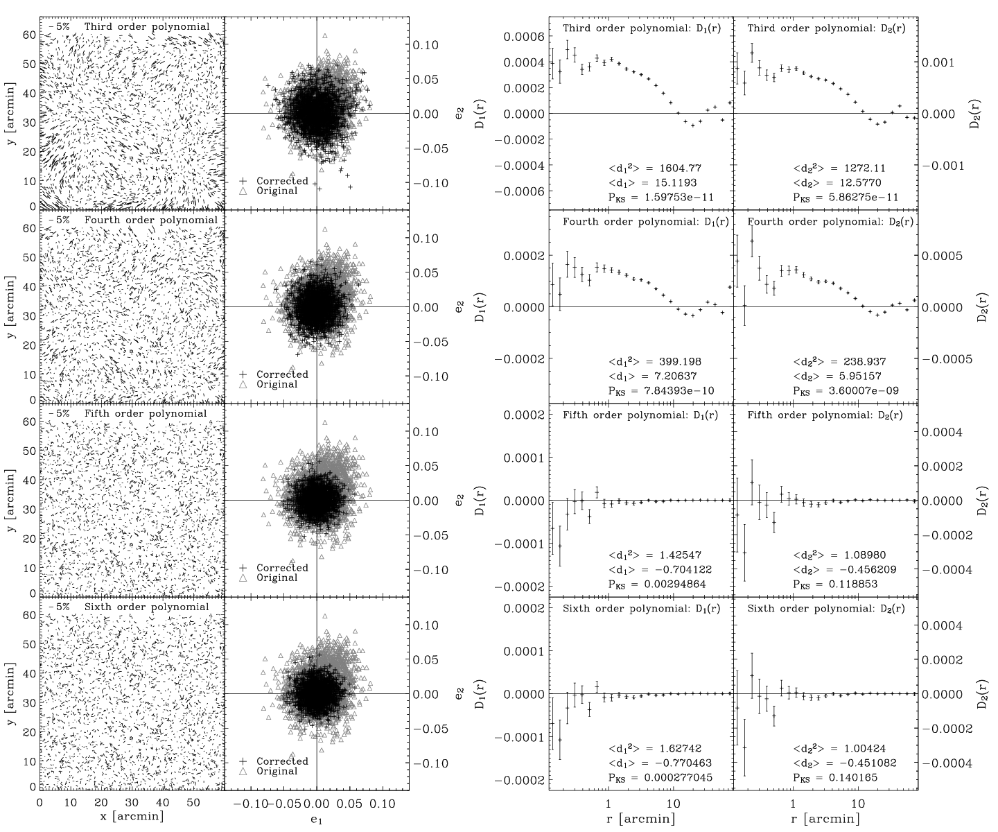
Having fit the 2500 simulated starfield measurements of $e$ using a set of models $e_{\mbox{\scriptsize$\mathrm{m}$}}(\mbox{\boldmath$x$};f_{\mbox{\scriptsize$\mathrm{m}$}})$, for a variety of different fitting schemes $f_{\mbox{\scriptsize$\mathrm{m}$}}$, the diagnostic functions $D_{1}(r)$ and $D_{2}(r)$ are calculated using the formula in equation (5). Measurements are divided into 25 logarithmically-spaced angular bins between 7 arcsec and 1.4 deg. This binning scheme was chosen as fairly representing both small and large scale information. By varying these values it was also verified that $D_{1}(r)$ and $D_{2}(r)$ were stable in regards to this choice, which was found to be true once sufficient numbers of bins were used as to be able to explore small scale correlations. Uncertainties were then calculated as the standard error upon the mean value from all the pairs within each bin, therefore not taking the correlation in values between neighbouring bins into account. Calculations of the $D_{1}(r)$ and $D_{2}(r)$ diagnostics, for each scheme $f_{\mbox{\scriptsize$\mathrm{m}$}}$, can be seen in the right hand panels of Figure 4 for the global fit and Figure 5 for the chipwise fit.

Whilst it should be noted that residual-residual correlations have already been used by some groups to rule out or justify PSF models (see, e.g., Hoekstra, 2004; Van Waerbeke et al., 2005; Hoekstra et al., 2006; Schrabback et al., 2007), and that these will be compared to $D_{1}(r)$ and $D_{2}(r)$ in the following Section, the left hand panels of Figures 4 & 5 show comparative examples of more simple diagnostics used in the past to display the results of PSF model fits (see, e.g., Hoekstra et al., 1998; Heymans et al., 2005; Schrabback et al., 2007). The far left hand panels of Figures 4 & 5 show ‘whisker plots’ of $e-e_{\mbox{\scriptsize$\mathrm{m}$}}$ (referred to as corrected ellipticities) to depict the random nature of fitting residuals. As can be seen by comparison with the corresponding $D_{1}(r)$ plots, correlation and anticorrelation may exist that is difficult to accurately quantify by eye, although qualitatively there are traces of correlation in the third and fourth order fit whisker plots. A correlation analysis of some sort is nonetheless clearly desirable, just as has been argued previously (Hoekstra, 2004). The inner left hand panels depict the distribution of ‘original’ ellipticities $e$ in comparison to the distribution of the corrected ellipticities $e-e_{\mbox{\scriptsize$\mathrm{m}$}}$; once again these plots are more difficult to quantifiably interpret than $D_{1}(r)$ and $D_{2}(r)$, which show more markedly different behaviour with $f_{\mbox{\scriptsize$\mathrm{m}$}}$. The question remains as to whether these new diagnostics are behaving as predicted in Section 2.

Examining first the global fit results shown in Figure 4 it can be seen that both $D_{1}(r)$ and $D_{2}(r)$ show clear residual positive and negative correlations for the underfitting models, as predicted. Both diagnostics appear to be broadly consistent with zero for the fifth and sixth order fits. For the chipwise fits of Figure 5 the results are similar but show an interesting extra feature. While both diagnostics rule out a first order chipwise fit as clearly underfitting, and the second order more marginally, the third order chipwise fit shows slight evidence of anticorrelation on small scales. This is then seen more clearly when the fit is taken to sixth order chipwise, particularly for the $D_{1}(r)$ diagnostic. These results suggest an overfit to the data for third and sixth order chipwise fits, at least according the reasoning presented in Section 2.4: this is a reasonable conclusion given knowledge of the number of degrees of freedom in the initial model, and could not have been so easily diagnosed using current methods.

Furthermore, the fact that neither the second nor third order chipwise fits show perfect consistency with zero suggests that none of the schemes chosen in this artificial chipwise splitting of the field is best suited to modelling the data, also a reasonable conclusion. However, it may be that this apparent inconsistency is instead caused by chance and the fact that $\left\langle m^{*}m\right\rangle(\mbox{\boldmath$r$})$ is no longer isotropic, since the artificial chips are rectangular. Nonetheless, even the possibility that $D_{1}(r)$ and $D_{2}(r)$ might allow general modelling schemes to be iteratively improved by correcting flaws such as the wrong choice of fitting function family, or the unnecessary splitting into independent chips, is of practical interest when fitting to an $e_{\mbox{\scriptsize$\mathrm{t}$}}$ of unknown functional form. Fitting to an arbitrary underlying field using a ‘wrong’ (or, more accurately, incomplete) basis will be explored further in Section 5, in which polynomial fits will be made to randomly generated fields with only an average power spectrum specified.

In summary, for the simple example presented in Figure 4, it appears that the degree of agreement with $D_{1}(r)=D_{2}(r)=0$ is a potentially useful aid to model selection when compared with simple diagnostic tools that have been used in the past. In Figure 5 both diagnostics help rule out models that would clearly be under- or overfitting, but there is no scheme that performs perfectly once the field is artificially split into chips. This fact gives hope that correlation analyses of this sort might guide, in a directed manner, iterative improvements to modelling where there is no clear physical motivation for selecting a given scheme (in the case presented it might motivate the decision not to model chipwise, for example). It is now instructive to compare the results of this analysis with the more complex diagnostics of PSF modelling that have been discussed in the literature, which are also based upon correlations in residuals, to see what may be added by the approach presented here.

The use of residual correlation diagnostics in a similar form to $D_{1}(r)$ and $D_{2}(r)$ is not new, having been advocated by Hoekstra (2004) in the form of the aperture mass dispersion estimator $\mathcal{M}(r)$ defined in equation (16) of Schneider et al. (2002) (see also Crittenden et al., 2002; Schneider, Van Waerbeke & Mellier, 2002), a filtered combination of $\xi_{+}(r)$ and $\xi_{-}(r)$ that gives an unbiased estimator of the cosmological aperture mass dispersion:

and

where the functions $T_{\pm}(x)$ are non-zero only for $x<2$ and are given in Schneider, Van Waerbeke & Mellier (2002). The aperture mass dispersion has the useful property that it allows a decomposition into ‘E’ and ‘B’ mode contributions (which are $\left\langle M^{2}_{\textrm{ap}}\right\rangle(r)$ and $\left\langle M^{2}_{\perp}\right\rangle(r)$ respectively) to the correlation signal, the former of which only is produced by a simple scalar mass potential (although B-modes can be created by contamination to the shear correction, intrinsic alignments of source galaxies etc., see Schneider, 2006). This measure was then employed by Van Waerbeke et al. (2005) and Hoekstra et al. (2006) to find optimal schemes for modelling the spatial variation of the PSF anisotropy, aiming towards $\mathcal{M}(r)=0$ for the residuals between modelled and measured PSF anisotropies. In both studies the chosen PSF fitting scheme was that which minimized the aperture mass dispersion of its residuals.

In Figure 6 the aperture mass dispersion is plotted for the residuals of the fits described in Sections 3.2 & 3.3, corresponding to the diagnostics plotted in Figures 4 & 5. The results are similar to those of $D_{1}(r)$ and $D_{2}(r)$, in that there are clear correlations for the underfitting cases. The signal to noise is reduced, a known feature of this statistic (e.g., Hoekstra et al., 2006; Schneider, 2006; Fu et al., 2008), and a means of positively identifying overfitting versus underfitting is less clear. This is because the aperture mass filtering of $\xi_{+}(r)$ and $\xi_{-}(r)$, which provides a desirably clean statistic when considering lensing due to physical mass distributions, makes the interpretation of correlated modelling residuals (via simple arguments such as those presented in Section 2) more complicated. One can say that correlation or anticorrelation exists, but saying which and why is less clear.

There is a suggestion in the bottom right hand side panel of Figure 6, for the sixth order chipwise fit, that the negative values of $\left\langle M^{2}_{\textrm{ap}}\right\rangle_{E/B}$ are an indication of the overfitting model in the same way as the negative values of $D_{1}(r)$ and $D_{2}(r)$ at small scales; although with apparently less overall signal than $D_{1}(r)$. Justifying this hypothesis using extensions to the arguments of Section 2 may be possible, and would immediately identify a clearly overfitting PSF model in the study performed by Hoekstra et al. (2006) (Figure 7 of that work): a not impossible finding given their independent fitting of second order polynomials to each of 36 chips across the CFHTLS Megacam field. Whether this sheds more insight than $D_{1}(r)$ and $D_{2}(r)$ upon the PSF model quality is unclear, however, and even unlikely given the lower signal to noise of the aperture mass measures (although see Fu & Kilbinger, 2009).

Nevertheless, as $\left\langle M^{2}_{\textrm{ap}}\right\rangle$ (or the more recently-derived ring statistics $\left\langle\mathcal{R}\mathcal{R}\right\rangle_{E/B}$, see Schneider & Kilbinger, 2007; Eifler, Schneider & Krause, 2009; Fu & Kilbinger, 2009) provides a model-independent method for E/B mode decomposition, it is in many ways a preferred choice for constraining cosmological parameters. Therefore, it will undoubtedly be of use to express residual correlations in the PSF model in terms of such quantities to quantify the contamination to the measured shear signal (e.g., Hoekstra, 2004; see also Section 6). But in the diagnosis of poor modelling, and in the directed manner in which simplifications or increases in complexity to the PSF model can be motivated, the interpretational clarity of $D_{1}(r)$ and $D_{2}(r)$ is an advance upon the use of the aperture mass dispersion.

Schrabback et al. (2007) also present a residual correlation analysis as a diagnostic of PSF modelling. These authors demonstrate that their chosen PSF model minimized the two functions $|\xi_{+}(r)+\xi_{-}(r)|$ and $|\xi_{+}(r)-\xi_{-}(r)|$ when measured upon model-data stellar ellipticity residuals, after randomly drawing stars from dense stellar fields (estimating the impact upon cosmic shear by scaling to an equivalent shear correction using randomly-drawn $P^{g}$ values from a galaxy population; see Schrabback et al., 2007). Overfitting was not a concern for these authors, who built a family of robust and detailed HST PSF models using dense stellar fields and then selected from this family via a maximum-likelihood match to the far fewer stars available in the galaxy survey images. As such, no attempt was made to interpret the sign of the resulting functions and the absolute values alone sufficed as a diagnostic. Again, the interpretability of $D_{1}(r)$ and $D_{2}(r)$ in terms of over- and underfitting, via the arguments in Section 2, is of significant additional value.

These results are interesting, but in order to test their repeatability it will be necessary to find some method of compressing the data and quantifying the qualitative visual appraisal so far conducted. Ideally there would be a means of ascribing a single, easily-calculated number to the $D_{1}(r)$ and $D_{2}(r)$ results, describing how well a given model matches the desired $D_{i}(r)=0$ behaviour. An obvious example is a chi-squared-like measure, but a true chi-squared is impossible without knowledge of the covariance between bins of $D_{i}(r)$, and these covariance matrices may in general only be estimated post hoc (often imperfectly) via a statistical jackknife or bootstrap. The calculation of even a single $D_{1}(r)$ or $D_{2}(r)$ takes some short time, varying with the square of the number of data points, and so these processor-intensive bootstrap techniques quickly become prohibitively expensive. In this Section we examine practical possibilities for a cheaper alternative to a full chi-squared measure of the $D_{i}(r)=0$ hypothesis.

To assign simple numbers to these results, in effect searching for a better proxy to the ‘appraisal-by-eye’ performed in the previous Section, the following quantities are defined:

Here $i=1,2$ so as to specify the $D_{1}(r)$ or $D_{2}(r)$ diagnostic respectively, $j$ denotes each discrete bin of angular scale $r_{j}$, and the error estimate on each $D_{i}(r_{j})$ is denoted as $\sigma_{D_{i}}(r_{j})$. As discussed above, it should be noted that the values for neighbouring bins of $D_{i}(r)$ are correlated and the uncertainties $\sigma_{D_{i}}(r_{j})$ do not take this into account: it would thus be dangerous to associate equation (41) with any sort of true chi-squared measure of the goodness of fit to a desired $D_{i}=0$ scenario.

However, use may be made of the fact that the correlation between bins for the diagnostics must be expected to be minimized for those successful models that approach $D_{i}=0$: this can be simply argued by considering that $m$ is expected to become approximately random in these cases. Also of use is the fact that the most important task at hand is merely to select a best-fitting model using a single number that quantifies this success. It might still be hoped that (40) and (41) are useful as a way of ranking competing models. The overall normalization of $\left\langle d_{i}\right\rangle$ and $\left\langle d^{2}_{i}\right\rangle$ for failing cases would, when ranking, be less important than the relative normalization as compared to successful cases.

Another means of quantifying the agreement with $D_{i}(r)=0$ is via the the Kolmogorov-Smirnov (KS) test (see, e.g., Press et al., 1992; Lupton, 1993), suggested to the grateful author by the anonymous referee. In the null hypothesis of a well-fitting model we may approximate that the individual values of $(d_{i})_{j}$ are each independently described by a Gaussian distribution with zero mean and unit variance. The maximal difference between the empirical cumulative distribution function (derived from the data) and the cumulative distribution function of the null hypothesis can then be used to assess the goodness of fit. The probability $P_{\textrm{KS}}(d_{i})$ that the null hypothesis could produce at least the maximal difference seen may then be calculated from a series approximation to the Kolmogorov distribution (although note that the use of this distribution is not strictly accurate, given that the ‘data’ $(d_{i})_{j}$ we use are derived quantities, and so this measure should be rightly interpreted only as an approximate guide; see Press et al., 1992).

The values of each of the $\left\langle d_{i}\right\rangle$, $\left\langle d^{2}_{i}\right\rangle$ and $P_{\textrm{KS}}(d_{i})$ statistics, for each fit to the starfield, are given in Figures 4 & 5. It would be naively expected that the best fitting $f_{\mbox{\scriptsize$\mathrm{m}$}}$ would show minimum values of $\left\langle d^{2}_{i}\right\rangle$ and $|\left\langle d_{i}\right\rangle|$, and a maximum $P_{\textrm{KS}}(d_{i})$: this is seen in the case of $D_{1}(r)$, but the $D_{2}(r)$ results marginally favour the overfitting sixth order polynomial in this case. All statistics strongly rule out lower order fits. For the chipwise fits the situation is more complex, due to their being no fitting model which shows clear consistency with $D_{i}(r)=0$. Second and third order fits are variously preferred. As discussed in Section 3.3, this is perhaps due to there being no $f_{\mbox{\scriptsize$\mathrm{m}$}}$ in this artificially split case that can reproduce all features of the ellipticity field without some overfitting redundancy.

All three statistics show some promise in being able to approximately describe the extent to which $D_{i}(r)=0$. More sophisticated approaches could certainly be explored, particularly given the information regarding the expected signatures of under- and overfitting described in Sections 2.3 & 2.4. This extra information might be perhaps be used within a Bayesian framework to select models, particularly if the modeller wished to rule out either an under- or overfitting model at any cost. This may be fertile ground for future work, as it is clear that the three statistics $\left\langle d^{2}_{i}\right\rangle$, $|\left\langle d_{i}\right\rangle|$, and $P_{\textrm{KS}}(d_{i})$ were chosen above all for their immediate simplicity and clarity.

These results lead to the possibility of asking another question: can model selection via the statistics described here be successfully repeated for a variety of input $e_{\mbox{\scriptsize$\mathrm{t}$}}$ fields? A single example field is hardly strong evidence for the utility of $D_{1}(r)$ and $D_{2}(r)$ in more general cases, so many more fields must be tested. The broad success of the three simplifying statistics described in this Section offers hope that the author might be spared from the need to visually inspect many plots of $D_{1}(r)$ and $D_{2}(r)$, and avoid the inevitable subjectivity in such an approach. Moreover, the necessity and difficulty of performing a full and stable statistical jackknife calculation (in order to estimate covariances) may be avoided. The following Section tests the success of $\left\langle d_{i}^{2}\right\rangle$, $|\left\langle d_{i}\right\rangle|$ and $P_{\textrm{KS}}(d_{i})$ as criteria for correctly identifying appropriate modelling order using a large number of randomly generated $e_{\mbox{\scriptsize$\mathrm{t}$}}$ anisotropy fields.

The number of times a global fitting scheme of order $m$ was chosen as best representing the simulated starfield of input order $n$ is shown in Figure 7, quantifying the success of the $\left\langle d^{2}_{i}\right\rangle_{\mbox{\scriptsize$\mathrm{min}$}}$, $|\left\langle d_{i}\right\rangle|_{\mbox{\scriptsize$\mathrm{min}$}}$ and $P_{\textrm{KS}}^{\mbox{\scriptsize$\mathrm{max}$}}(d_{i})$ criteria for this simple Monte Carlo test. The same results are shown for the chipwise fits in Figure 8.

For the range of input models and statistics tested it appears that $D_{1}(r)$ is typically a cleaner and more reliable model selection diagnostic than $D_{2}(r)$, which in both the global and chipwise fits is noisier and appears to show a biased relative preference for overfitting models in most cases. $\left\langle d^{2}_{1}\right\rangle_{\mbox{\scriptsize$\mathrm{min}$}}$ and $|\left\langle d_{1}\right\rangle|_{\mbox{\scriptsize$\mathrm{min}$}}$ show striking success in selecting the correct fitting order in Figure 7, but not so their $D_{2}(r)$ counterparts. The performance of $P^{\mbox{\scriptsize$\mathrm{max}$}}_{\textrm{KS}}(d_{i})$ is more disappointing overall and seems insensitive to identifying overfits when fitting globally, although in Figure 8 there is evidence of it correctly ruling out the more extreme chipwise overfits, at least for $D_{1}(r)$. $|\left\langle d_{1}\right\rangle|_{\mbox{\scriptsize$\mathrm{min}$}}$ appears to show moderate preference for lower order fits than $\left\langle d^{2}_{1}\right\rangle_{\mbox{\scriptsize$\mathrm{min}$}}$, particularly at lower orders, perhaps due to the close cancelling of correlation and anticorrelation on different scales (c.f. Section 2.3). Nonetheless, all statistics appear to rule out underfitting models successfully.

The chipwise results show better rejection of overfitting models, and therefore greater overall agreement between the results for different statistics. This is not surprising when one considers that for chipwise fits the number of degrees of freedom in the fitting model increases more rapidly with increasing order $m$ than in the global case. The comparison of the chipwise and global results therefore suggests that, for those statistics which failed to rule out overfits, the problem was more of relative sensitivity than a total failure. The $P_{KS}^{\mbox{\scriptsize$\mathrm{max}$}}(d_{i})$ statistic performs the worst, and Press et al. (1992) suggest a possible reason for this: the sensitivity of the KS test of deviations from the c.d.f.$(d_{i})$ is not independent of $d_{i}$, and is in fact most sensitive around the median value. This makes the test least sensitive in the wings of the probability distribution, and hence to the outliers which may give the clearest indication a poor fit. This is one plausible explanation, and Press et al. (1992) describe possible alternatives to the KS test that attempt to mitigate this problem. Another reason might be the incorrect use of the Kolmogorov distribution in the test, since $(d_{i})_{j}$ are quantities derived from the data rather than direct data themselves (see Section 3.5; also Press et al., 1992).

These results leave open an avenue for potentially valuable further study, as an optimal way for identifying $D_{1}(r)=D_{2}(r)=0$ is clearly not yet found. Despite this fact, the results of Figures 7 & 8 are extremely encouraging, for $\left\langle d^{2}_{1}\right\rangle_{\mbox{\scriptsize$\mathrm{min}$}}$ and $|\left\langle d_{1}\right\rangle|_{\mbox{\scriptsize$\mathrm{min}$}}$ in particular. The results $D_{2}(r)$ were generally less successful, and seemed to show an insensitivity to overfitting in particular. Possible reasons for this are now briefly discussed.

In the Monte Carlo tests performed it appears that the selection criteria based upon $D_{2}(r)$ show some shortcomings that need to be explored. Firstly, they often prefer overfitting models when compared to the $D_{1}(r)$ results (biased when compared to the truth for Figure 7). Secondly, both $\left\langle d^{2}_{2}\right\rangle$ and $|\left\langle d_{2}\right\rangle|$ are noisy. This latter can perhaps be partially explained by the fact that $D_{2}(r)$ is itself often more noisy than $D_{1}(r)$, a natural consequence of the value and variation of $e$ being typically larger than that of $e-e_{\mbox{\scriptsize$\mathrm{m}$}}$ (see equations 13 and 14); the biased results warrant further investigation.

Complete answers as to why $D_{2}(r)$ performed relatively poorly in this simple experiment almost certainly lie outside the capability of this paper, as this behaviour may depend non-trivially upon many factors. Possible contributions could be: the number of stars simulated per field; the overall signal to noise for the $e$ field; the geometry of the chosen field of view; the nature of the typical pattern described by the simulated $e_{\mbox{\scriptsize$\mathrm{t}$}}$ (the chosen polynomials, even when randomly generated, do not come close to being able to describe arbitrary surfaces); the degree of variance and covariance within and between bins of $D_{2}(r)$. Whilst all these factors may potentially be limiting in the correct circumstance, the last is worthy of some further discussion in particular as it is one aspect in which $D_{2}(r)$ may differ significantly from $D_{1}(r)$.

Evidence of overfitting is generally seen at small scales, and it has been seen that on large scales $D_{i}\simeq 0$ even for drastic overfits (e.g. Figure 5). At these scales the quoted errors upon $D_{2}(r)$ will still be large when compared to those for $D_{1}(r)$, because of the typically greater values of $e$ as compared to $e-e_{\mbox{\scriptsize$\mathrm{m}$}}$, meaning that contributions to $\left\langle d_{2}^{2}\right\rangle$ on these scales are overly suppressed. Moreover, the use of $\left\langle d_{i}^{2}\right\rangle$ as a means of ranking competing models will work best in situations where the covariance matrix is totally diagonal, and will correspond in such cases to a chi-squared-like measure of goodness of fit to $D_{i}=0$. Conversely, strong off-diagonal values might produce exactly the results seen in Figures 7 & 8 for the $D_{2}(r)$ diagnostics. If false, the assumption of weakly correlated uncertainties between bins, which is implicit for the utility of $\left\langle d^{2}_{i}\right\rangle$ and $|\left\langle d_{i}\right\rangle|$, will lend undue weight to the supposed success of $D_{i}=0$ on large scales and therefore undue credence to the overfitting model itself. If the covariance matrix for $D_{2}(r)$ contains significant off-diagonal terms, even in the case of a successful model, this may be cause for the systematic preference towards overfitting models seen in Figures 7 & 8.

In that case, however, it must also be seen if there is a systematic reason why the covariances of $D_{1}(r)$ and $D_{2}(r)$ differ in their diagonality. One important difference is apparent from the very definitions given in equations (13) and (14): the first diagnostic is the residual-residual autocorrelation, whilst the second is a measure of the data-residual cross-correlation. It may be that $D_{2}(r)$ will therefore suffer from strong covariances even for cases approaching $D_{2}(r)=0$, due to the physically correlated nature of the data $e$, whereas such correlations in $D_{1}(r)$ will inevitably decrease as the model tends towards $D_{1}(r)=0$. Another difference may lie in the angle averaging, performed over all pairs separated by distance $r$, implicit in the definition of the correlation functions thus far used in this paper (see, e.g., equations 3 and 5). It can be imagined that $D_{2}(r)$, being more strongly dependent upon the non-isotropic field $e_{\mbox{\scriptsize$\mathrm{t}$}}$, might suffer from greater uncertainty and even bias due to the angle averaging that is implicit in the way $D_{1}(r)$ and $D_{2}(r)$ are calculated.

These are plausible explanations for the effects seen but, unfortunately, this discussion will remain essentially un-concluded without further investigation. Estimating post hoc the covariance matrices of correlation functions such as $D_{2}(r)$ is expensive with current computing resources and, as the covariance of $D_{2}(r)$ will depend non-trivially upon the starfield $e_{\mbox{\scriptsize$\mathrm{t}$}}$, the calculation would need to be made many times within the current simulation framework. Pessimistically, even with such work we may in fact be learning more about the properties of any simulated $e_{\mbox{\scriptsize$\mathrm{t}$}}$ than about $D_{i}(r)$. Despite these issues regarding $D_{2}(r)$, it has certainly been demonstrated that both $D_{i}(r)$ show some potential for diagnosing modelling quality, and that $D_{1}(r)$ appears outstandingly successful in the tests so far conducted. A next step is to enlarge the space of potential $e_{\mbox{\scriptsize$\mathrm{t}$}}$ fields to include more general, arbitrary structure, and to see how $D_{1}(r)$ and $D_{2}(r)$ perform when a perfect fit may no longer be possible.

References

- Arfken & Weber (2005) Arfken G. B., Weber H. J., 2005, Mathematical methods for physicists 6th ed.
- Beckwith et al. (2006) Beckwith S. V. W., et al., 2006, AJ, 132, 1729
- Bernstein & Jarvis (2002) Bernstein G. M., Jarvis M., 2002, AJ, 123, 583
- Bridle et al. (2008) Bridle S., et al., 2008, ArXiv e-prints: astro-ph/0802.1214
- Crittenden et al. (2002) Crittenden R. G., Natarajan P., Pen U.-L., Theuns T., 2002, ApJ, 568, 20
- Efstathiou (2008) Efstathiou G., 2008, MNRAS, 388, 1314
- Eifler et al. (2009) Eifler T., Schneider P., Krause E., 2009, ArXiv e-prints: astro-ph/0907.2320
- Fu et al. (2008) Fu L., et al., 2008, A&A, 479, 9
- Fu & Kilbinger (2009) Fu L., Kilbinger M., 2009, ArXiv e-prints: astro-ph/0907.0795
- Gelman et al. (2003) Gelman A., Carlin J. B., Stern H. S., Rubin D. B., 2003, Bayesian Data Analysis, Second Edition. Chapman & Hall/CRC
- Heymans et al. (2005) Heymans C., et al., 2005, MNRAS, 361, 160
- Heymans et al. (2006) Heymans C., et al., 2006, MNRAS, 368, 1323
- Heymans et al. (2008) Heymans C., et al., 2008, MNRAS, 385, 1431
- Hoekstra (2004) Hoekstra H., 2004, MNRAS, 347, 1337
- Hoekstra (2007) Hoekstra H., 2007, MNRAS, 379, 317
- Hoekstra et al. (1998) Hoekstra H., Franx M., Kuijken K., Squires G., 1998, ApJ, 504, 636
- Hoekstra et al. (2005) Hoekstra H., Hsieh B. C., Yee H. K. C., Lin H., Gladders M. D., 2005, ApJ, 635, 73
- Hoekstra et al. (2006) Hoekstra H., Mellier Y., Van Waerbeke L., Semboloni E., Fu L., Hudson M. J., Parker L. C., Tereno I., Benabed K., 2006, ApJ, 647, 116
- Jarvis & Jain (2004) Jarvis M., Jain B., 2004, ArXiv e-prints: astro-ph/0412234
- Jarvis et al. (2008) Jarvis M., Schechter P., Jain B., 2008, ArXiv e-prints: astro-ph/0810.0027
- Kaiser (2004) Kaiser N., 2004, in J. M. Oschmann Jr. ed., Society of Photo-Optical Instrumentation Engineers (SPIE) Conference Series Vol. 5489 of Presented at the Society of Photo-Optical Instrumentation Engineers (SPIE) Conference, Pan-STARRS: a wide-field optical survey telescope array. pp 11–22
- Kaiser et al. (1995) Kaiser N., Squires G., Broadhurst T., 1995, ApJ, 449, 460
- Kurek & Szydłowski (2008) Kurek A., Szydłowski M., 2008, ApJ, 675, 1
- Leauthaud et al. (2007) Leauthaud A., et al., 2007, ApJS, 172, 219
- Liddle et al. (2006) Liddle A., Mukherjee P., Parkinson D., 2006, Astronomy and Geophysics, 47, 040000
- Liddle (2007) Liddle A. R., 2007, MNRAS, 377, L74
- Lupton (1993) Lupton R., 1993, Statistics in theory and practice. Princeton, N.J.: Princeton University Press, —c1993
- Mandelbaum et al. (2006) Mandelbaum R., Seljak U., Kauffmann G., Hirata C. M., Brinkmann J., 2006, MNRAS, 368, 715
- Massey et al. (2007a) Massey R., et al., 2007a, Nat, 445, 286
- Massey et al. (2007b) Massey R., et al., 2007b, MNRAS, 376, 13
- Massey & Refregier (2005) Massey R., Refregier A., 2005, MNRAS, 363, 197
- Ngan et al. (2008) Ngan W.-H. W., Van Waerbeke L., Mahdavi A., Heymans C., Hoekstra H., 2008, ArXiv e-prints: astro-ph/0809.3465
- Paulin-Henriksson et al. (2008) Paulin-Henriksson S., Amara A., Voigt L., Refregier A., Bridle S. L., 2008, A&A, 484, 67
- Paulin-Henriksson et al. (2009) Paulin-Henriksson S., Refregier A., Amara A., 2009, A&A, 500, 647
- Press et al. (1992) Press W. H., Teukolsky S. A., Vetterling W. T., Flannery B. P., 1992, Numerical recipes in FORTRAN. The art of scientific computing. Cambridge: University Press, —c1992, 2nd ed.
- Refregier (2003) Refregier A., 2003, MNRAS, 338, 35
- Refregier & Bacon (2003) Refregier A., Bacon D., 2003, MNRAS, 338, 48
- Rhodes et al. (2007) Rhodes J. D., Massey R. J., Albert J., Collins N., Ellis R. S., Heymans C., Gardner J. P., Kneib J.-P., Koekemoer A., Leauthaud A., Mellier Y., Refregier A., Taylor J. E., Van Waerbeke L., 2007, ApJS, 172, 203
- Sasiela (1994) Sasiela R. J., 1994, Electromagnetic wave propagation in turbulence. Evaluation and application of Mellin transforms
- Schneider (2006) Schneider P., 2006, in Meylan G., Jetzer P., North P., Schneider P., Kochanek C. S., Wambsganss J., eds, Saas-Fee Advanced Course 33: Gravitational Lensing: Strong, Weak and Micro Part 3: Weak gravitational lensing. pp 269–451
- Schneider & Kilbinger (2007) Schneider P., Kilbinger M., 2007, A&A, 462, 841
- Schneider et al. (2002) Schneider P., Van Waerbeke L., Kilbinger M., Mellier Y., 2002, A&A, 396, 1
- Schneider et al. (2002) Schneider P., Van Waerbeke L., Mellier Y., 2002, A&A, 389, 729
- Schrabback et al. (2007) Schrabback T., Erben T., Simon P., Miralles J.-M., Schneider P., Heymans C., Eifler T., Fosbury R. A. E., Freudling W., Hetterscheidt M., Hildebrandt H., Pirzkal N., 2007, A&A, 468, 823
- Schrabback et al. (2009) Schrabback T., et al., 2009, ArXiv e-prints: astro-ph/0911.0053
- Smith et al. (2003) Smith R. E., Peacock J. A., Jenkins A., White S. D. M., Frenk C. S., Pearce F. R., Thomas P. A., Efstathiou G., Couchman H. M. P., 2003, MNRAS, 341, 1311
- Spergel et al. (2007) Spergel D. N., et al., 2007, ApJS, 170, 377
- Tian et al. (2009) Tian L., Hoekstra H., Zhao H., 2009, MNRAS, 393, 885
- Trotta (2008) Trotta R., 2008, Contemporary Physics, 49, 71
- Van Waerbeke et al. (2005) Van Waerbeke L., Mellier Y., Hoekstra H., 2005, A&A, 429, 75