Acoustic vibrations of anisotropic nanoparticles
Abstract
Acoustic vibrations of nanoparticles made of materials with anisotropic elasticity and nanoparticles with non-spherical shapes are theoretically investigated using a homogeneous continuum model. Cubic, hexagonal and tetragonal symmetries of the elasticity are discussed, as are spheroidal, cuboctahedral and truncated cuboctahedral shapes. Tools are described to classify the different vibrations and for example help identify the modes having a significant low-frequency Raman scattering cross-section. Continuous evolutions of the modes starting from those of an isotropic sphere coupled with the determination of the irreducible representation of the branches permit some qualitative statements to be made about the nature of various modes. For spherical nanoparticles, a more accurate picture is obtained through projections onto the vibrations of an isotropic sphere.
I Introduction
The lowest frequency vibrations of isolated nanoparticles are in the THz range, on the order of the speed of sound divided by the dimension. These are commonly refered to as confined acoustic phonons and are unrelated to optical phonons. There have been numerous experimental and theoretical studies on the acoustic vibrations of nanoparticles in the last few decades. These vibrations have been observed by a variety of experimental techniques including low frequency Raman scattering,[1] time resolved femtosecond pump-probe experiments,[2, 3, 4] infrared absorption,[5, 6] inelastic neutron scattering[7] and persistent spectral hole burning.[3]
Reasonable estimates for the mode frequencies are obtained using the 1882 Lamb solution of the continuum elastic problem for an elastically isotropic, homogeneous, free sphere.[8] This provided sufficiently good agreement to confirm that confined acoustic phonon modes were really being observed. However, this model was unable to deal with the anisotropy of actual samples.
Recent advances have permitted the creation of high quality elastically anisotropic samples.[9] The essential features are (1) a narrow size distribution (2) good crystallinity so that a significant amount of nanoparticles in the sample are mono-domain (3) controlled shape of nanoparticles and (4) separation of nanoparticles so that they vibrate as independent units. As a result, the vibrational modes of elastically anisotropic nanoparticles have been observed. This has created the need for an alternative to the Lamb model capable of dealing with nanoparticles with lower symmetry.
In this work, we use the method of Visscher et al.[10] which is a standard numerical approach suitable for the calculation of the frequencies and the wavefunctions of the vibrations of such nanoparticles. The symmetry of these modes, their volume variation and their Lamb mode parentage are determined and applied to the prediction of their observation by different experimental techniques such as inelastic light scattering.
II Methods
The situation for an isotropic nanoparticle will now be summarized. In this case, the system is spherically symmetric. Thus, vibrational modes can be classified by their angular momentum number and its -component . Modes can also be classified either as torsional (T) or spheroidal (S). Finally, modes are also indexed in order of frequency by ( corresponds to the first harmonic (fundamental mode), to the second harmonic and so on). In the following, we will indicate Lamb modes using the compact notation X where X=S or X=T.
All modes can be observed by inelastic neutron scattering in the typical situation where the wavelength of the neutrons is much smaller than the nanoparticle size. For nanoparticles whose dimension is small compared to the wavelength of light (dipolar approximation), Raman only detects S0 and S2, infrared absorption only detects S1[11] and time-resolved femtosecond pump-probe experiments typically only detect S0. In the following, we will assume that the nanoparticles are small enough so that the dipolar approximation holds.
Nanoparticles with either isotropic or anisotropic elasticity will be considered in the following. Isotropic elasticity is considered mainly for comparison with previous studies. Anisotropic elasticity is used for perfect nanocrystals consisting of a single domain. We will refer to such nanoparticles as being “mono-domain” in the following. In a small nanoparticle, a mono-domain structure is not necessarily energetically favorable. For example, it is well known that multiply-twinned silver nanoparticles are much more stable for certain ranges of size.[12]
II.1 Calculation of frequencies and associated displacements
The frequencies and their associated displacements for an anisotropic nanoparticle have been calculated using the approach introduced by Visscher et al.[10] which also assumes continuum elasticity. Other authors have already confirmed that the convergence of this method is faster than the convergence of finite element methods at least in some cases.[13] The relevance of continuum elasticity for nanoparticles has been confirmed using atomistic calculations[14, 15, 16, 17] for nanoparticles larger than 2-3 nm and even for ZnO nanoparticles for which surface relaxation and stress are significant.[18] Most of the results presented in this paper have been obtained for nanospheres whose diameter is 10 nm which is well above these limits. It is possible to extrapolate them to different sizes since the frequencies vary as the inverse diameter. However care should be taken not to consider very small nanoparticles for which surface effects could significantly alter the validity of the continuum approximation. The calculational method for the modes gives each mode in terms of power series coefficients so that:
| (1) |
The power expansion covered for good convergence for all the modes we are interested in. The frequencies for the isotropic spherical case were reproduced with very good accuracy. The convergence for strongly anisotropic systems is harder to check. Despite checking that the frequencies do not significantly change when adding more terms to the power expansion, we also compared the calculated frequencies with the Finite Element Mesh Sequence method introduced in a previous work.[19]
In this work, all the displacements have been normalized according to equation 2 where is the volume of the nanoparticle.[20]
| (2) |
II.2 Group theory
II.2.1 Degeneracy lifting
In the absence of spherical symmetry, modes are classified according to their remaining symmetry. For example, for a spherical nanoparticle with cubic elasticity, such as Ag, Au and Si, the system is symmetric under the symmetry operations of a cube, which is the 48-element group .
Our calculations return a large number of modes which have to be considered to interpret inelastic light scattering spectra or other experimental results. It is important to use not only the frequencies but also the wavefunctions in order to do that. Group theory is a very valuable tool in this context as it allows for example to identify the Raman active modes and therefore simplify the assignment process. In this work, we will only consider nanoparticles whose dimensions are small compared to the wavelength of light (dipolar approximation) in order to discuss the selection rules of Raman scattering. Table 1 shows how the degeneracy of the Raman and infrared active modes of an isotropic sphere[11] is lifted or not when lowering the symmetry. Only point groups relevant for the rest of this paper are considered.
| point group | S0 | S1 | S2 | S3 | S4 |
|---|---|---|---|---|---|
| O | A | T | E + T | A + T + T | A + E + T + T |
| D | A | A + E | A + B + B + E | A + B + B + 2 E | 2 A + A + B + B + 2 E |
| D | A | A + E | A + E + E | A + B + B + E + E | A + B + B + E + 2 E |
| D | A | A + E | A + E + E | A + E + E + E | A + E + E + E + E |
II.2.2 Numerical determination of the irreducible representations
In order to take full advantage of group theory, it is important to label the different modes with the corresponding irreducible representation. Sophisticated and specific approaches could be considered to restrict the calculations to modes having a well-defined symmetry. However, we preferred to keep the numerical approach detailed previously because it is more general. We added a few calculation steps to determine the irreducible representation from the wavefunctions. It turns out this can be achieved very reliably and without much additional calculation time.
being a symmetry operation of the point group of concern, and with a full set of eigenmodes having the same frequency, the character of for this irreducible group of vibrations is:
| (3) |
Such integrals can be calculated accurately and quickly when each Cartesian component of the displacement field is a sum of terms of the form . By calculating a few well-chosen characters, it is then straightforward to distinguish all the different irreducible representations using the character table of the point group. The only restriction to apply this procedure is that the degeneracy must be known and therefore the convergence must be good. Of course, a more general approach is require to handle accidental degeneracies.
In the following we detail some additional ways to improve our knowledge of these vibrations. These are needed since regarding Raman scattering many modes are labeled as Raman active due to the irreducible representation they belong to. However there is not necessarily an efficient coupling mechanism enabling a significant Raman intensity. The following tools are designed to somewhat address this problem.
II.3 Volume variation
The volume of the nanoparticle does not change for every possible vibration. For isotropic spherical nanoparticles, the volume changes only for the spheroidal vibration. This volume change is also involved in the time-resolved femtosecond pump-probe measurements.[2] As a result, it is interesting to calculate it for all the vibrations.
The volume variation corresponds to the flux of the displacement through the surface of the particle. The expression for a dimensionless volume variation is given in equation 4. Using the divergence theorem, this 2D integral can be turned into a volume integral involving derivatives of functions which are already calculated in the frame of Visscher’s method.[10] Therefore this quantity can also be accurately and efficiently calculated. It can be shown that the volume variation is different from zero for fully symmetric vibrations only, i.e. for A vibrations for the symmetries considered here.
| (4) |
Of course, the value of depends on the normalization (see equation 2).
II.4 Smooth variation of parameters
In order to follow how the vibrations evolve when lowering the symmetry, it is possible to follow the frequencies of the different modes while slowly varying the parameters (for example the shape or the elastic constants of the material the nanoparticle is made of). The curve representing the variation of one frequency is called a branch in the following. Group theory can help plotting such branches more reliably because all the different points on a given branch share the same irreducible representation. Moreover branches having different irreducible representations can cross but not branches having the same irreducible representation. This originates from the coupling between the different branches being due to the anisotropy itself whose irreducible representation is A for the point groups we focus on. As a result, all modes having a given irreducible representation belong to the same branch and can be safely connected.
In this work, branches due to varying elastic anisotropy are calculated by changing the stiffness tensor using with , being the tensor of the isotropic material (which can be obtained by averaging the sound velocities[19] or other methods[21] or using measured longitudinal and transverse sound velocities) and the anisotropic tensor. The parameters used in this work are given in Ref. 22. It should be noted that such branches are made of fictive materials except for where the real elastic parameters of the bulk material are used.
II.5 Projections
When the lowering of the symmetry is not due to a change in the shape of the nanoparticle, it is possible to compare the wavefunctions (omitting their time dependences) of the two systems. As commonly done for atomistic calculations[14, 15, 16], we calculated the projection of the displacements of spherical nanoparticles onto Lamb modes. For a given mode whose displacement is the projection onto the Lamb mode is defined as:
| (5) |
The orthonormality and completeness of the Lamb modes implies that, for any ,
| (6) |
Likewise, the orthonormality and completeness of the modes of the anisotropic nanoparticle implies that, for any , and ,
| (7) |
However, a more relevant quantity is obtained by summing the squared projections over all the degenerate Lamb modes i.e. over . As a result, the total squared projection of onto the subspace spanned by the modes X is:
| (8) |
III Applications
III.1 Spherical nanocrystals with cubic crystallinity
III.1.1 Spherical mono-domain silver and gold nanoparticles
Let us first consider the case of a spherical nanoparticle made of silver. This nanoparticle is mono-domain and therefore the stiffness tensor is the same everywhere inside the nanoparticle and identical to that of bulk silver.[23] Table 2 presents the calculated frequencies, irreducible representations, main projections onto the modes of an isotropic silver sphere and volume variations of the lowest frequency modes. The six modes have zero frequency and correspond to the rigid rotations and translations of the nanoparticle. The branches corresponding to the lowering of the symmetry when going from the isotropic to the anisotropic case are plotted in figure 1.
| (GHz) | i.r. | Squared Lamb projections | ||
|---|---|---|---|---|
| 7-8 | 103.3 | E | 0.995 S + 0.002 S + … | 0.0 |
| 9-11 | 106.8 | T | 0.936 T + 0.054 S + … | 0.0 |
| 12 | 151.1 | A | 0.996 T + 0.002 S + … | 0.0 |
| 13-15 | 153.0 | T | 0.499 S + 0.480 S + … | 0.0 |
| 16-17 | 161.0 | E | 0.974 T + 0.018 T + … | 0.0 |
| 18-20 | 169.4 | T | 0.821 S + 0.160 T + … | 0.0 |
| 21-23 | 196.4 | T | 0.758 T + 0.178 S + … | 0.0 |
| 24-26 | 196.9 | T | 0.411 T + 0.369 S + … | 0.0 |
| 27-28 | 211.2 | E | 0.838 S + 0.113 S + … | 0.0 |
| 29-31 | 221.8 | T | 0.748 T + 0.199 S + … | 0.0 |
| 32-34 | 232.1 | T | 0.466 S + 0.466 S + … | 0.0 |
| 35-37 | 234.5 | T | 0.665 S + 0.127 T + … | 0.0 |
| 38 | 248.9 | A | 0.959 S + 0.028 S + … | 0.4 |
| … | … | … | … | … |
| 75 | 331.2 | A | 0.930 S + 0.039 S + … | 4.3 |
| … | … | … | … | … |

Figure 1 clearly shows that the introduction of elastic anisotropy significantly lifts the degeneracy of most modes. One notable exception is the breathing mode which corresponds to the second A branch. This mode is non-degenerate and its frequency hardly changes with anisotropy. The other important exception are the dipolar modes S1 which are infrared active and transform into T with the same degeneracy. The lowest Raman active mode S which has degeneracy 5 is split into the lowest E and T branches ( and in table 2 respectively) as expected from table 1. These anisotropic modes have a dominant projection onto S confirming their Lamb mode parentage.
Similar calculations have been performed for mono-domain gold nanoparticles using the elastic constants from Ref. 24 and the results are presented in table 3 and figure 2. Compared to the previous case of silver, only the values of the stiffness tensor were changed so most observations previously made still apply. We recently reported on the experimental observation of the splitting of S for such nanoparticles.[9] There is an excellent agreement between these measurements and the splitting calculated using the present approach. This strongly supports the validity of our approach and in particular the relevance of elastic anisotropy even in such very small nanoparticles.
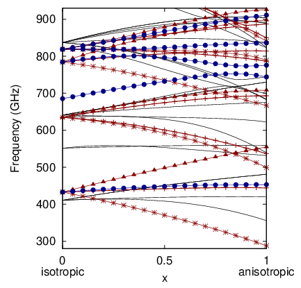
One notable difference between gold and silver concerns the case of the breathing mode. The isotropic breathing mode at 311.6 GHz belongs to the third A branch. Therefore it is tempting to assume that the anisotropic breathing mode lies on the same branch and is therefore mode at 301.9 GHz. However, table 3 reveals that mode is a much better candidate for a breathing mode due to its larger volume variation and projection onto S. It turns out this is due to a strong mixing of the A branches as anisotropy is increased. Indeed, the isotropic modes S4, S6 and S8 are split into various irreducible representations, one of them being A. Unlike the previous case of silver, the elastic constants of gold result in four A branches coming from S, S, S and S being in the same frequency range. As a result, mode which is the mode having the strongest projection onto S and also has a large volume variation does not lie on the same branch as S. Figure 3 shows the variation of the squared projections onto S of three of these A branches as the elastic anisotropy is varied and confirm the mixing discussed above.
| (GHz) | i.r. | Squared Lamb projections | ||
|---|---|---|---|---|
| 7-8 | 74.6 | E | 0.996 S + 0.002 S + … | 0.0 |
| 9-11 | 76.9 | T | 0.939 T + 0.053 S + … | 0.0 |
| 12 | 109.0 | A | 0.996 T + 0.002 S + … | 0.0 |
| 13-15 | 111.2 | T | 0.516 S + 0.466 S + … | 0.0 |
| 16-17 | 114.1 | E | 0.977 T + 0.016 T + … | 0.0 |
| 18-20 | 120.5 | T | 0.837 S + 0.146 T + … | 0.0 |
| 21-23 | 140.2 | T | 0.773 T + 0.162 S + … | 0.0 |
| 24-26 | 141.8 | T | 0.433 T + 0.356 S + … | 0.0 |
| 27-28 | 154.0 | E | 0.824 S + 0.126 S + … | 0.0 |
| 29-31 | 158.9 | T | 0.698 T + 0.259 S + … | 0.0 |
| 32-34 | 168.2 | T | 0.617 S + 0.186 T + … | 0.0 |
| 35-37 | 169.7 | T | 0.484 S + 0.456 S + … | 0.0 |
| … | … | … | … | … |
| 43 | 182.0 | A | 0.987 S + 0.005 S + … | 0.1 |
| … | … | … | … | … |
| 118 | 285.8 | A | 0.594 S + 0.218 S + … | 1.2 |
| … | … | … | … | … |
| 133 | 301.9 | A | 0.866 S + 0.049 S + … | 0.3 |
| … | … | … | … | … |
| 141 | 310.1 | A | 0.806 S + 0.133 S + … | 3.9 |
| … | … | … | … | … |
| 183 | 341.5 | A | 0.378 S + 0.319 S + … | 1.4 |
| … | … | … | … | … |

Similar but less pronounced mixings are observed in all cases. The density of modes (i.e. the number of modes per unit frequency) increases with frequency. As a result, the probability of mixings increases with frequency or . This explains why the lowest frequency modes such as the lowest E ones are almost pure isotropic modes (S). However, the lowest T branches which are issued from the same S and from T are already significantly mixed by anisotropy for both gold and silver nanoparticles. This is clearly evidenced in figure 3 too.

III.1.2 Raman scattering efficiency for metallic cubic materials
Low-frequency Raman scattering from silver and gold nanoparticles has attracted a lot of attention during the last few decades. The scattering mechanisms have been identified[25] and one might wonder how the anisotropic considerations detailed in this work fit into this picture. The inelastic light scattering process for such nanoparticles is mediated by the dipolar plasmon. As a result only scattering by S0 and S2 modes is allowed[11] and has a significant Raman scattering cross-section[25] in the isotropic case. Anisotropic nanoparticles obey the same rules and one might qualitatively estimate their Raman intensity by using the projections onto the same isotropic modes. As a result a significant scattering intensity is expected for the lowest E and T modes of both silver and gold while the second T mode should have a small Raman cross-section due to its small projection onto S. The volume mechanism enables a measurable Raman intensity for the A modes having a significant projection onto S0, i.e. for modes and for silver and gold respectively. The Raman intensity for other A modes should be very weak and probably not measurable in practice.
III.1.3 Other cubic materials
For cubic materials, the degree of elastic anisotropy is quantified by the Zener anisotropy ratio, = . = for an isotropic material. Silver and copper both have and also had the largest mode splittings that we found. For comparison, we mention results for some less anisotropic materials. For a silicon nanosphere with radius 5 nm, the Lamb mode S splits into two frequencies at 386.6 GHz (E) and 485.9 GHz (T). For a germanium nanosphere, the same mode is split into 235.1 GHz (E) and 295.3 GHz (T). Using the standard deviation as a simple measure of the frequency splitting (and therefore neglecting the effect of mixings), we obtain 23, 22, 10 and 11% for Ag, Au, Si and Ge respectively. For all these commonly studied materials, this splitting cannot be neglected.
III.2 Spherical nanocrystals with tetragonal crystallinity
Nanospheres with tetragonal crystallinity have a lower symmetry than the previous nanospheres with cubic crystallinity. The corresponding point group is D. As a result, more degeneracy lifting occurs. This results in a splitting of the infrared active S1 mode into A and E and four branches starting from the S mode (A, B, B and E). The relative order of these branches depends on the stiffness tensor. Two nanospheres made of TiO2 with radius 5 nm will be considered using the parameters from Ref. 26. One of them has the anatase crystal structure (table 4) and the other the rutile structure (table 5 and figure 4). We used these calculations for the anatase crystal structure in a recent work[7] to model the inelastic scattering of neutrons. Both have tetragonal symmetry but different elastic parameters. This results in different relative positions of the frequencies of the modes coming from a given isotropic mode.
Using the same measure as before, the frequency splitting for the S modes is 10 and 20% for the anatase and rutile structure respectively.
Due to the lowering of the symmetry compared to the cubic case, the breathing mode is also susceptible to more mixings. For anatase TiO2, the S mode mixes mainly with T (mode ) while for rutile TiO2 it mixes mainly with S (mode ).
| (GHz) | i.r. | Squared Lamb projections | ||
|---|---|---|---|---|
| 7 | 283.5 | A | 0.977 S + 0.016 S + … | 0.6 |
| 8-9 | 284.0 | E | 0.931 T + 0.054 S + … | 0.0 |
| 10 | 298.5 | A | 0.999 T + 0.000 T + … | 0.0 |
| 11 | 304.3 | B | 0.998 T + 0.001 S + … | 0.0 |
| 12-13 | 316.1 | E | 0.996 S + 0.002 T + … | 0.0 |
| 14 | 326.9 | B | 0.992 S + 0.008 T + … | 0.0 |
| 15 | 330.9 | B | 0.967 T + 0.027 S + … | 0.0 |
| 16 | 381.5 | B | 0.965 S + 0.033 T + … | 0.0 |
| 17 | 432.4 | A | 0.494 S + 0.436 S + … | 0.0 |
| 18 | 443.3 | B | 0.950 T + 0.028 S + … | 0.0 |
| 19-20 | 445.7 | E | 0.612 S + 0.323 S + … | 0.0 |
| 21 | 447.6 | A | 0.537 S + 0.448 S + … | 0.0 |
| 22-23 | 455.5 | E | 0.957 T + 0.015 S + … | 0.0 |
| 24-25 | 463.4 | E | 0.758 S + 0.220 S + … | 0.0 |
| 26 | 470.7 | A | 0.989 T + 0.005 T + … | 0.0 |
| 27 | 473.9 | B | 0.865 T + 0.060 S + … | 0.0 |
| 28 | 476.9 | B | 0.987 S + 0.008 T + … | 0.0 |
| 29-30 | 480.7 | E | 0.941 T + 0.031 S + … | 0.0 |
| 31 | 510.9 | B | 0.946 S + 0.026 T + … | 0.0 |
| 32-33 | 537.1 | E | 0.826 S + 0.095 S + … | 0.0 |
| 34 | 573.8 | A | 0.974 S + 0.009 S + … | 0.0 |
| 35 | 580.8 | A | 0.910 S + 0.030 S + … | 0.8 |
| … | … | … | … | … |
| 55 | 678.4 | A | 0.885 S + 0.082 T + … | 0.2 |
| … | … | … | … | … |
| 67 | 743.1 | A | 0.803 S + 0.156 T + … | 4.0 |
| … | … | … | … | … |
| 69 | 751.6 | A | 0.675 T + 0.162 S + … | 1.8 |
| … | … | … | … | … |
| (GHz) | i.r. | Squared Lamb projections | ||
|---|---|---|---|---|
| 7 | 288.1 | B | 0.978 S + 0.013 T + … | 0.0 |
| 8 | 296.9 | B | 0.943 T + 0.045 S + … | 0.0 |
| 9-10 | 355.8 | E | 0.693 T + 0.150 S + … | 0.0 |
| 11 | 419.8 | A | 0.981 T + 0.013 T + … | 0.0 |
| 12-13 | 444.1 | E | 0.927 S + 0.062 T + … | 0.0 |
| 14 | 453.1 | A | 0.955 S + 0.035 S + … | 0.8 |
| 15 | 481.0 | B | 0.965 T + 0.033 S + … | 0.0 |
| 16 | 499.4 | B | 0.715 T + 0.210 S + … | 0.0 |
| 17-18 | 531.7 | E | 0.402 S + 0.288 T + … | 0.0 |
| 19-20 | 537.1 | E | 0.813 T + 0.071 S + … | 0.0 |
| 21 | 539.4 | A | 0.465 T + 0.327 S + … | 0.0 |
| 22 | 555.0 | B | 0.997 S + 0.001 S + … | 0.0 |
| 23 | 558.9 | A | 0.969 S + 0.016 S + … | 0.0 |
| 24 | 600.0 | B | 0.845 S + 0.095 T + … | 0.0 |
| 25-26 | 622.3 | E | 0.575 S + 0.247 S + … | 0.0 |
| … | … | … | … | … |
| 38 | 744.0 | A | 0.739 S + 0.157 S + … | 1.4 |
| 39-40 | 744.2 | E | 0.725 S + 0.178 S + … | 0.0 |
| 41 | 775.8 | A | 0.631 S + 0.269 S + … | 4.1 |
| … | … | … | … | … |
| 50 | 836.1 | A | 0.439 S + 0.351 S + … | 1.6 |
| … | … | … | … | … |
| 62 | 911.0 | A | 0.739 S + 0.169 S + … | 0.9 |
| … | … | … | … | … |
| 81 | 1019.1 | A | 0.649 T + 0.110 S + … | 0.5 |
| … | … | … | … | … |
III.3 Spherical nanocrystals with hexagonal crystallinity
As a last example of the influence of elastic anisotropy, we focus on nanospheres made of crystals having hexagonal symmetry, namely CdSe (table 6 and figure 5 using the elastic constants from Ref. 27), Co (table 7 using the elastic constants from Ref. 28) and ZnO (elastic constants from Ref. 18). The associated point group is D. The most notable difference compared to previous symmetries is that some “accidental” degeneracy exists for such systems: for each B (B) vibration there is a B (B) vibration having the same frequency.
Using the same measure as before, the frequency splitting for the S modes is 9, 11 and 5% for the CdSe, Co and ZnO respectively. ZnO is therefore the most elastically isotropic amongst the materials studied in this work.
Regarding the breathing mode, for CdSe it is hardly mixed with other modes due to anisotropy and results in mode which has a strong projection onto S and a large volume variation. For the nanosphere made of cobalt, there is a strong mixing with the S and S modes and the anisotropic mode with the largest projection onto S and the largest volume variation is mode which is on the branch coming from S at 466.7 GHz and not on the branch starting from S at 536.8 GHz.
The infrared active S mode which was recently observed[6] for CdSe nanoparticles is split by the lowering of symmetry into A and E modes at 181.9 and 181.3 GHz respectively. This frequency splitting is very small but these modes mix with the branches having identical irreducible representations coming from S. Neglecting this mixing, the isotropic S is in excellent agreement with the anisotropic description.
| (GHz) | i.r. | Squared Lamb projections | ||
|---|---|---|---|---|
| 7 | 119.4 | A | 1.000 T + 0.000 T + … | 0.0 |
| 8-9 | 123.2 | E | 0.998 T + 0.001 S + … | 0.0 |
| 10-11 | 126.8 | E | 0.999 S + 0.001 T + … | 0.0 |
| 12-13 | 132.6 | E | 0.998 S + 0.002 T + … | 0.0 |
| 14-15 | 132.8 | E | 0.971 T + 0.023 S + … | 0.0 |
| 16 | 158.6 | A | 0.999 S + 0.001 S + … | 0.0 |
| 17-18 | 181.3 | E | 0.894 S + 0.103 S + … | 0.0 |
| 19 | 181.9 | A | 0.789 S + 0.206 S + … | 0.0 |
| 20 | 186.1 | A | 0.999 T + 0.001 T + … | 0.0 |
| 21-22 | 189.2 | B+B | 0.994 T + 0.004 S + … | 0.0 |
| 23-24 | 192.1 | E | 0.998 S + 0.001 T + … | 0.0 |
| 25-26 | 193.5 | E | 0.980 T + 0.014 S + … | 0.0 |
| 27-28 | 198.1 | B+B | 0.996 S + 0.004 T + … | 0.0 |
| 29-30 | 208.0 | E | 0.947 T + 0.042 S + … | 0.0 |
| 31-32 | 214.7 | E | 0.870 S + 0.099 S + … | 0.0 |
| 33 | 226.7 | A | 0.789 S + 0.206 S + … | 0.0 |
| … | … | … | … | … |
| 55 | 273.8 | A | 0.926 S + 0.060 S + … | 0.3 |
| 56 | 284.9 | A | 0.999 T + 0.001 T + … | 0.0 |
| 57 | 296.0 | A | 0.925 S + 0.059 S + … | 0.2 |
| … | … | … | … | … |
| 77 | 320.4 | A | 0.985 S + 0.011 S + … | 4.5 |
| … | … | … | … | … |

| (GHz) | i.r. | Squared Lamb projections | ||
|---|---|---|---|---|
| 7-8 | 229.8 | E | 0.998 T + 0.001 T + … | 0.0 |
| 9 | 232.2 | A | 1.000 T + 0.000 T + … | 0.0 |
| 10-11 | 240.7 | E | 0.997 S + 0.003 T + … | 0.0 |
| 12-13 | 246.6 | E | 1.000 S + 0.000 T + … | 0.0 |
| 14-15 | 251.4 | E | 0.942 T + 0.029 S + … | 0.0 |
| 16 | 316.1 | A | 0.996 S + 0.003 S + … | 0.0 |
| 17-18 | 334.7 | E | 0.919 S + 0.063 S + … | 0.0 |
| 19 | 346.4 | A | 0.828 S + 0.167 S + … | 0.0 |
| … | … | … | … | … |
| 49 | 497.8 | A | 0.958 S + 0.042 S + … | 4.5 |
| … | … | … | … | … |
III.4 Non-spherical nanocrystals
In order to illustrate the usefulness of the same numerical tools for a different source of anisotropy, we consider in the following the lowering of the symmetry due to the shape of the nanoparticles. We start with a minor change of the shape as the nanosphere is transformed into a spheroid having an isotropic elasticity. Then we consider faceted nanoparticles with elastic anisotropy.
III.4.1 Spheroids with isotropic elasticity
Let us consider a spheroid made of silver with a degenerate semi-axis nm and a varying non-degenerate semi-axis . We assume the elasticity to be isotropic. The point group associated with such a spheroid is therefore D. The frequencies, irreducible representations and volume variations for a spheroid with nm are presented in table 8. The branches obtained for varying are presented in figure 6.
Let us now focus on the effect of the spheroidal deformation on the S modes. Looking at the displacements corresponding to these modes for small deviations from the sphere, it is possible to understand the frequency variations. The lowest A mode corresponds to a stretching along the direction accompanied by a shrinking in the plane. Therefore it can be seen as a vibration confined along the direction and its frequency varies roughly as . The E vibrations correspond to a stretching in the plane without changes along the axis and therefore their frequencies hardly changes with . The E vibrations correspond to a stretching in the and plane without changes along the axis and therefore their frequencies vary with a slower eccentricity dependence than the previous mode. These rough approximations are in agreement with the dependence observed in figure 6.
Using perturbation theory,[29] it is possible to obtain more accurate expressions for the frequencies of these three branches. The exact variations for are , and for the E, E and A modes respectively where and is the frequency of modes S for a spherical particle having the same volume. Note that the length of the degenerate semi-axis is constant in this work and therefore the volume varies linearly with . Using results in expressions which are in very good agreement with figure 6 close to .
| (GHz) | i.r. | ||
|---|---|---|---|
| 7-8 | 62.4 | E | 0.0 |
| 9 | 71.1 | A | 0.0 |
| 10 | 90.8 | A | 0.4 |
| 11-12 | 103.8 | E | 0.0 |
| 13 | 116.6 | A | 0.0 |
| 14-15 | 127.0 | E | 0.0 |
| 16-17 | 136.3 | E | 0.0 |
| … | … | … | … |
| 34 | 185.2 | A | 0.2 |
| … | … | … | … |
| 57 | 244.6 | A | 1.0 |
| … | … | … | … |
| 64 | 253.3 | A | 0.0 |
| … | … | … | … |
| 90 | 294.8 | A | 4.5 |
| … | … | … | … |
| 110 | 318.8 | A | 0.5 |
| … | … | … | … |

Regarding the “breathing” mode, the picture gets very complicated when differs significantly from 1. S is on the 4 A branch. Therefore the mode of the spheroid with on the same branch is mode . However, due to the mixing with neighboring A branches, the mode with is a better candidate since its volume variation is much larger. Thanks to this additional property of the symmetric modes, it is therefore possible to follow the breathing mode. However, because it is not possible to project onto the Lamb modes of an isotropic sphere due to the different shapes, only the branches and the anti-crossing patterns between branches having the same irreducible representation can help tracking qualitatively the other S and T modes.
These calculations are targetted at interpreting experimental results on silver nanoparticles such as nanocolumns.[30] Compared to previous calculations using the FEMS method presented before,[31] the current approach enables a more complete description of the different vibrations besides being faster and more acurate. In particular, the variation of volume is very efficient in showing which modes should be observed by time-resolved pump-probe experiments.[4] It is interesting to note that some works[30, 4] concern aligned nanocolumns which results in interesting depolarization rules for the Raman peaks. For non-aligned nanoparticles, these rules are the same as those used routinely for an ensemble of molecules, i.e. all the Raman active modes produce completely depolarized Raman peaks except for the A vibrations which have a “polarized” scattering for which the Raman peak is more intense when the polarizations of the incident and scattered photons are parallel. For oriented nanoparticles, this rule doesn’t hold and the angles of the incident and scattered photons with respect to the axis of symmetry of the nanoparticles have to be taken into account.
Recent time-resolved pump-probe femtosecond experiments for single gold nanoparticles[32] also demonstrate the need for such a model. In particular, the observation of a peak close to the S frequency is reported for spheroids but not for spheres. This is in agreement with the features reported here for silver, namely that the A mode coming from the S mode has a non-zero volume variation enabling it to be observed in such an experiment unlike the S mode of a sphere. It is also worth noting that the shape of the peak attributed to “the breathing mode” in this work for dumbbells looks quite complicated. Such nano-objects have the same symmetry as spheroids. As a result, in most cases there is no such thing as a “breathing mode” but rather a set of A vibrations in a relatively narrow frequency range having a significant volume variation. This is due to the fact that the A branch coming from the S vibration mixes with all the other A branches which come from all the Sℓ vibrations with even . Modeling such gold dumbbells is beyond the scope of this paper, but doing so would enable a more detailed understanding of the experimental results, especially for such single particle measurements for which the external shape of the nanoparticles can be obtained from SEM images. The relatively large size of these nanoparticles prevents them from being single-domain and justifies the use of the isotropic elastic approximation.
III.4.2 anisotropic gold polyhedra
Observation of faceted nanoparticles using electron microscopy is quite common. Such facets can be thought of as a signature of the inner crystal structure and therefore as an indication of the elastic anisotropy.[33] To quantify the importance of the shape on the vibrations, we calculated the frequencies and irreducible representations for some polyhedra and the results are presented in table 9. The crystal lattice is oriented with respect to the shape so that the [100] planes correspond to the square faces for the cuboctahedron and to the octagonal faces for the truncated cuboctahedron. There is no lowering of symmetry associated with these shapes compared to the case of a mono-domain spherical gold nanoparticle. The relevant point group is then D. While table 9 clearly shows that the lowest frequencies change with the shape, the frequencies of the lowest E and T modes are hardly affected. Since the degeneracies of the S0 and S1 modes are not lifted, all the modes which are observable by Raman scattering, infrared absorption of time-resolved pump-probe experiments are not sensitive to these changes of shape.
| i.r. | sphere | cuboctahedron | truncated cuboctahedron |
|---|---|---|---|
| E | 74.6 | 74.5 | 74.5 |
| T | 76.9 | 73.4 | 75.5 |
| A | 109.0 | 81.6 | 91.7 |
| T | 111.2 | 108.7 | 110.7 |
| E | 114.1 | 102.3 | 107.9 |
| T | 120.5 | 121.3 | 121.7 |
| T | 140.2 | 128.0 | 133.8 |
| … | … | … | … |
IV Multiple-domain nanoparticles
Several attempts have been made in the past either to fit low frequency Raman spectra or to determine the size distribution of the nanoparticles inside a sample using the shape of the low-frequency Raman peak. Both approaches always rely on the validity of the isotropic model by Lamb and on the predominance of the size distribution, the coupling with a surrounding matrix and the electron-vibration coupling to fit the broadening of the peaks. However the distribution of internal structures of multiple-domain nanoparticles also results in inhomogeneous broadening.
It is in principle possible to model the vibrations of a multiple-domain nanoparticle using the numerical method of Visscher et al.. However this requires a complete description of the position of the domain boundaries and the orientations of the crystal lattice. For ensemble measurements with the nanoparticles having a variety of different internal structure, a lot of calculations would be required. Otherwise, using such an approach for a single internal structure is justified only if all the studied nanoparticles are identical for ensemble measurements or if the inner structure of a nanoparticle studied in a single particle measurement is perfectly known. Due to these latter two conditions having never been met until now and also to the additional complexity of modelling a multiple-domain nanoparticle, we suggest using the isotropic approximation to describe an ensemble of multiple-domain nanoparticles. What this means is that no nanoparticle behaves exactly as an isotropic nanoparticle, but the isotropic approximation gives an average value due to the nanoparticles having essentially random domain structures. Ensemble measurements should therefore show features associated with these average frequencies with some inhomogeneous width due to the inhomogeneous distribution of domains inside the population of nanoparticles.
We calculated the vibrations of an icosahedron made of gold and silver assuming the isotropic approximation to be valid in that case. The corresponding point group for such a nanoparticle is I. It is interesting to note that in this case there is no degeneracy lifting for the modes S0, S1 and S2 whose irreducible representation in the new system is A, T and H respectively. As a result, there is hardly any frequency difference compared to the case of a sphere having the same volume. A real icosahedron made of an anisotropic material but having the same symmetry due to the presence of twins would have no degeneracy lifting either for the same modes and we expect almost the same frequencies too.
V Conclusion
We have presented mode frequencies and irreducible representations for homogeneous continuum nanoparticles using a standard numerical method which can handle arbitrary shape and anisotropic elasticity. The classification by irreducible representation makes it possible to label many modes as either Raman or infrared inactive. We have been able to go beyond this to provide some tools to make qualitive estimates of the Raman intensity of potentially Raman active modes. These tools are well-suited for the interpretation of experimental results obtained with vibrational spectroscopies.[9, 7]
This approach fills a large gap in current works since up to now it was necessary to choose between a simplified spherical isotropic model where the underlying physics was simple enough but where the accuracy was challenged by recent experimental results or a numerical approach which provides accurate frequencies but which is inefficient in practice due to the lack of tools to distinguish the relevant vibrations without complex simulations of spectra.
It is clear that additional theoretical work is required in order to quantitatively predict Raman intensities for elastically anisotropic modes of spheres. However, the labeling of modes via their Lamb mode parentage by continuous variation of the elastic isotropy and projections for spherical nanoparticles, is a powerful descriptive and semi-quantitative tool for understanding what is going on with elastic anisotropy. The significant frequency splittings obtained in this work call into question the validity of the isotropic approximation for the case of multiple-domain nanoparticles. Such systems are very relevant experimentally but their vibrations remain largely unaddressed.
Acknowledgements.
LS acknowledges Professor Eugène Duval for stimulating discussions and comments. DBM acknowledges support from NSERC of Canada.References
- [1] E. Duval, A. Boukenter, and B. Champagnon, Phys. Rev. Lett. 56, 2052 (1986).
- [2] N. Del Fatti, C. Voisin, F. Chevy, F. Vallée, and C. Flytzanis, J. Chem. Phys. 110, 11484 (1999).
- [3] M. Ikezawa, J. Zhao, A. Kanno, and Y. Masumoto, J. Phys. Soc. Japan 74, 3082 (2005).
- [4] J. Burgin, P. Langot, A. Arbouet, J. Margueritat, J. Gonzalo, C. N. Afonso, F. Vallée, A. Mlayah, M. D. Rossell, and G. Van Tendeloo, Nano Lett. 8, 1296 (2008).
- [5] D. B. Murray, C. H. Netting, L. Saviot, C. Pighini, N. Millot, D. Aymes, and H.-L. Liu, J. Nanoelectron. Optoelectron. 1, 92 (2006a).
- [6] T.-M. Liu, J.-Y. Lu, H.-P. Chen, C.-C. Kuo, M.-J. Yang, C.-W. Lai, P.-T. Chou, M.-H. Chang, H.-L. Liu, Y.-T. Li, et al., Appl. Phys. Lett. 92, 093122 (2008).
- [7] L. Saviot, C. H. Netting, D. B. Murray, S. Rols, A. Mermet, A.-L. Papa, C. Pighini, D. Aymes, and N. Millot, Phys. Rev. B 78, 245426 (2008).
- [8] H. Lamb, Proc. London Math. Soc. 13, 189 (1882).
- [9] H. Portalès, N. Goubet, L. Saviot, S. Adichtchev, D. B. Murray, A. Mermet, E. Duval, and M.-P. Piléni, Proc. Natl. Acad. Sci. U.S.A 105, 14784 (2008).
- [10] W. M. Visscher, A. Migliori, T. M. Bell, and R. A. Reinert, J. Acoust. Soc. Am. 90, 2154 (1991).
- [11] E. Duval, Phys. Rev. B 46, 5795 (1992).
- [12] S. Ino, J. Phys. Soc. Japan 27, 941 (1969).
- [13] P. R. Heyliger, E. Pan, S. Cook, and M. Manaloto, J. Sound and Vibration 311, 184 (2008).
- [14] W. Cheng, S.-F. Ren, and P. Y. Yu, Phys. Rev. B 71, 174305 (2005a).
- [15] W. Cheng, S.-F. Ren, and P. Y. Yu, Phys. Rev. B 72, 059901(E) (2005b).
- [16] N. Combe, J. R. Huntzinger, and A. Mlayah, Phys. Rev. B 76, 205425 (2007).
- [17] F. Ramirez, P. R. Heyliger, A. K. Rappé, and R. G. Leisure, J. Acoust. Soc. Am. 123, 709 (2008).
- [18] N. Combe, P.-M. Chassaing, and F. Demangeot, Phys. Rev. B 79, 045408 (2009).
- [19] L. Saviot, D. B. Murray, and M. C. Marco de Lucas, Phys. Rev. B 69, 113402 (2004).
- [20] D. B. Murray and L. Saviot, Phys. Rev. B 69, 094305 (2004).
- [21] A. N. Norris, J. of Mechanics of Materials And Structures 1, 223 (2006).
- [22] Mass densities in g.cm-3 and in GPa used in this work. Ag: , isotropic , , anisotropic , , . Au: , isotropic , , anisotropic , , . Si: , anisotropic , , . Ge: , anisotropic , , . isotropic TiO2: , , . Rutile TiO2: , anisotropic , , , , , . Anatase TiO2: , anisotropic , , , , , . CdSe: , isotropic , , anisotropic , , , , . Co: , isotropic , , anisotropic , , , , . ZnO: , anisotropic , , , , .
- [23] J. R. Neighbours and G. A. Alers, Phys. Rev. 111, 707 (1958).
- [24] R. F. S. Hearmon, in The elastic constants of crystals and other anisotropic materials, edited by K. H. Hellwege and A. M. Hellwege (Springer-Verlag, Berlin, 1984), vol. 18, supplement to III/11 of Landolt-Börstein New-Series, Group III.
- [25] G. Bachelier and A. Mlayah, Phys. Rev. B 69, 205408 (2004).
- [26] M. Iuga, G. Steinle-Neumann, and J. Meinhardt, Eur. Phys. J. B 58, 127 (2007).
- [27] E. Rabani, J. Chem. Phys. 116, 258 (2002).
- [28] P. Gangopadhyay, T. R. Ravindran, K. G. M. Nair, S. Kalavathi, B. Sundaravel, and B. K. Panigrahi, Appl. Phys. Lett. 90, 063108 (2007).
- [29] G. Mariotto, M. Montagna, G. Viliani, E. Duval, S. Lefrant, E. Rzepka, and C. Mai, Europhys. Lett. 6, 239 (1988).
- [30] J. Margueritat, J. Gonzalo, C. N. Afonso, A. Mlayah, D. B. Murray, and L. Saviot, Nano Lett. 6, 2037 (2006).
- [31] D. B. Murray, A. S. Laarakker, and L. Saviot, phys. stat. sol. (c) 3, 3935 (2006b).
- [32] A. L. Tchebotareva, M. A. van Dijk, P. V. Ruijgrok, V. Fokkema, M. H. S. Hesselberth, M. Lippitz, and M. Orrit, ChemPhysChem 10, 111 (2009).
- [33] B. Stephanidis, S. Adichtchev, S. Etienne, S. Migot, E. Duval, and A. Mermet, Phys. Rev. B 76, 121404 (2007).