\docnumCERN-PH-EP/2009-006 {Authlist}
T. Anticic15, B. Baatar6, J. Bartke4, L. Betev8, H. Białkowska14, C. Blume7, B. Boimska14, J. Bracinik1,a, V. Cerny1, O. Chvala11,b, J. Dolejsi11, V. Eckardt10, H.G. Fischer8, Z. Fodor3, P. Foka5, V. Friese5, M. Gaździcki7, C. Höhne5, K. Kadija15, A. Karev8, V. Kolesnikov6, M. Kowalski4, M. Kreps1,c, M. Makariev13, A. Malakhov6, M. Mateev12, G. Melkumov6, M. Mitrovski7, S. Mrówczyński9, R. Renfordt7, M. Rybczyński9, A. Rybicki4, A. Sandoval5, N. Schmitz10, P. Seyboth10, G. Stefanek9, R. Stock7, H. Ströbele7, T. Susa15, P. Szymanski14, V. Trubnikov14, D. Varga2, G. Vesztergombi3, D. Vranić5, S. Wenig8,Z. Włodarczyk9, A. Wojtaszek9
(The NA49 Collaboration)
1Comenius University, Bratislava, Slovakia
2 Eötvös Loránt University, Budapest, Hungary
3KFKI Research Institute for Particle and Nuclear Physics, Budapest, Hungary
4H. Niewodniczański Institute of Nuclear Physics,
Polish Academy of Sciences, Cracow, Poland
5Gesellschaft für Schwerionenforschung (GSI), Darmstadt, Germany.
6Joint Institute for Nuclear Research, Dubna, Russia.
7Fachbereich Physik der Universität, Frankfurt, Germany.
8CERN, Geneva, Switzerland
9Institute of Physics Świȩtokrzyska Academy, Kielce, Poland.
10Max-Planck-Institut für Physik, Munich, Germany.
11Charles University, Faculty of Mathematics and Physics, Institute of
Particle and Nuclear Physics, Prague, Czech Republic
12Atomic Physics Department, Sofia University St. Kliment Ohridski, Sofia, Bulgaria
13Institute for Nuclear Research and Nuclear Energy, BAS, Sofia, Bulgaria
14Institute for Nuclear Studies, Warsaw, Poland
15Rudjer Boskovic Institute, Zagreb, Croatia
anow at School of Physics and Astronomy, University of Birmingham, Birmingham, UK
bnow at UC Riverside, Riverside, CA, USA
cnow at Institut fur Experimentelle Kernphysik, Karlsruhe, DE
to be published in EPJC
New data on the production of protons, anti-protons and neutrons in p+p interactions are presented. The data come from a sample of 4.8 million inelastic events obtained with the NA49 detector at the CERN SPS at 158 GeV/c beam momentum. The charged baryons are identified by energy loss measurement in a large TPC tracking system. Neutrons are detected in a forward hadronic calorimeter. Inclusive invariant cross sections are obtained in intervals from 0 to 1.9 GeV/c (0 to 1.5 GeV/c) in transverse momentum and from -0.05 to 0.95 (-0.05 to 0.4) in Feynman x for protons (anti-protons), respectively. integrated neutron cross sections are given in the interval from 0.1 to 0.9 in Feynman x. The data are compared to a wide sample of existing results in the SPS and ISR energy ranges as well as to proton and neutron measurements from HERA and RHIC.
1 Introduction
In the framework of its extensive experimental programme concerning soft hadronic interactions at SPS energies, the NA49 collaboration has recently published detailed data on the inclusive production of charged pions in p+p collisions [1]. The present paper extends this study to the baryonic sector by providing inclusive cross sections for protons, anti-protons and neutrons. The aim is again to obtain precise sets of data covering the available phase space as densely and completely as possible in accordance with the available event statistics and the limitations set by the NA49 detector layout.
As in the case of pions, the experimental situation in the SPS energy range is far from being satisfactory also for baryons. The presently available data sets suffer from insufficient coverage and at least partially large systematic and statistical error margins. It is therefore one of the main aims of this study to provide a concise overview and evaluation of the experimental situation on a quantitative basis.
This paper is arranged as follows. The present experimental situation is discussed in Sect. 2. Section 3 concentrates on those aspects of the NA49 experiment which are special to baryon detection, as for instance high momentum tracking and neutron calorimetry. The acceptance coverage and the binning scheme are presented in Sect. 4, followed by the description of charged particle identification in Sect. 5. The evaluation of invariant cross sections and of the applied corrections is given in Sect. 6. Results concerning double differential cross sections for protons and anti-protons are presented in Sect. 7, followed by a detailed comparison to existing data in Sects. 8 and 9. Sections 10 and 11 show integrated results for protons and neutrons including a comparison to other experiments. Finally in Sect. 12 the NA49 results on proton and neutron production are compared to baryon production in deep inelastic lepton scattering from HERA.
2 The Experimental Situation
Concerning the present publication we are interested in the available measurements of the double differential cross section of identified baryons,
| (1) |
as a function of the phase space variables defined in this paper as transverse momentum and reduced longitudinal momentum
| (2) |
where denotes the longitudinal momentum component in the cms.
Defining a range of beam momenta from 100 to about 400 GeV/c as SPS/Fermilab energy range, quite a few experiments have published inclusive particle yields [2, 3, 4, 5, 6, 7, 8, 9, 10]. The corresponding data coverage of the / plane is shown in Fig. 1a for protons and in Fig. 1d for anti-protons. It is apparent from these plots that data are scarce in the regions of below 0.3 GeV/c and above 1 GeV/c as well as below 0.3. At large there is abundant coverage only for protons in a interval from about 0.2 to 0.6 GeV/c from experiments concentrating on single diffraction. It is therefore mandatory to also regard data from the ISR [11, 12, 13, 14, 15, 16, 17, 18, 19] at least in the overlapping region of up to 30 GeV for this comparison. The corresponding phase space regions are presented in Figs. 1b and 1e for protons and anti-protons, respectively. Except for a rather complete coverage at close to zero a lack of data in the intermediate region 0.1 0.4, at below 0.3 GeV/c and above about 1.5 GeV/c is evident.
The NA49 phase space coverage, Figs. 1c and 1f, is essentially only limited by counting statistics at large , and at large for the anti-protons. In addition there is a small phase space gap not accessible due to the interaction trigger, in a range below 0.05 GeV/c at = 0.6 to 0.4 GeV/c at = 0.95 which only concerns protons.
For neutrons, the situation is less favourable. There is only one measurement from Fermilab [20] and one ISR experiment [21, 22], with coverages shown in Fig. 1g and 1h. Due to lack of transversal granularity, the NA49 calorimeter only allows for the measurement of integrated neutron yields. The corresponding / coverage, limited by the fiducial dimension of the calorimeter, is shown in Fig. 1i.

It is useful to repeat here that the main aim of the present paper is to contribute precise new data covering the accessible phase space as densely and continuously as possible in a single experiment in order to clarify the unsatisfactory experimental situation and to provide a sound base for the comparative study of the more complex nuclear interactions.
3 The NA49 Experiment
The basic features of the NA49 detector have been described in detail in references [1, 23]. The top view shown in Fig. 2 recalls the main components.

The beam is defined by a CEDAR Cerenkov counter, several scintillation counters (S1, S2, V0) and a set of high precision proportional chambers (BPD1-3). The hydrogen target is placed in front of two superconducting Magnets (VTX1 and VTX2). Four large volume Time Projection Chambers (VTPC1 and VTPC2 inside the magnetic fields, MTPCL and MTPCR downstream of the magnets) provide for charged particle tracking and identification. A smaller Time Projection Chamber (GTPC) placed between the two magnets together with two Multiwire Proportional Chambers (VPC1 and VPC2) in forward direction allows tracking in the high momentum region through the gaps between the principal track detectors. A Ring Calorimeter (RCal) closes the detector setup 18 m downstream of the target.
As details of the beam and target setup, the trigger definition as well as the event and track selection have been given in [1] only those parts of the detector which are of special interest for the present paper will be described here. This concerns in particular the extension of the acceptance into the large region and the neutron calorimetry.
3.1 Tracking at high momenta using the GTPC and VPC’s
The particles originating from the primary interaction vertex and missing, at high momentum, the main TPC arrangement, are detected in the GTPC and VPC’s. These three sets of points are sufficiently far from each other to provide a reasonable lever arm for momentum measurement. A sketch of this detector part is shown in Fig. 3. For experimental details see [24].

The VPC proportional chambers feature a single sense wire plane with strip readout (30 degree inclination) on both cathode surfaces resulting in a space resolution of 2 mm. This results, together with the GTPC resolution of less than 150 m, in a longitudinal momentum resolution of

| (3) |
where the error is dominated by the VPC position resolution. The momentum resolution at maximum momentum was controlled using a trigger on beam particles. For inelastic events, it is also established by the width of the diffractive peak as shown in the raw distribution in Fig. 4.
The general improvement of charged particle acceptance at 0.4 due to this detector combination, as compared to the tracks visible in the main TPC detector only, is also apparent from Fig. 4.
The corresponding transverse momentum resolution is given by
| (4) |
It is dominated by both the GTPC and the transverse vertex resolutions. The resulting uncertainty of 30 MeV/c at beam momentum is small enough to allow the extraction of transverse momentum distributions up to the kinematic limit.
3.2 Neutron detection
Forward neutrons as well as fast forward charged particles are detected in the Ring Calorimeter (RCal). This device, originally designed for the study of jet production in deep inelastic interactions by the CERN NA5 experiment [25, 26, 27], is placed 18 m downstream of the target. It is a cylindrical structure with azimuthal and radial subdivision into 240 cells, each with an electromagnetic and hadronic compartment.
For the present purpose, it was off-centered with respect to the beam axis such that a fully sensitive fiducial area of 80160 cm2 corresponding to the size of the VPC chambers could be established, see Fig. 2. This corresponds to a cut-off of 1.25 GeV/c at = 0.2, increasing to more than 2 GeV/c at 0.4, for neutral particles.
Each RCal cell is built up from 2 parts: an electromagnetic part (20 radiation lengths of Pb/scintillator sandwich) and a hadronic part (4 interaction lengths of Fe/scintillator sandwich) [26]. Energy deposits in the two parts are recorded separately. As the position resolution of the RCal is rather limited in the transverse plane due to the substantial cell size, only integrated distributions are presented in this paper. For experimental details see [24].
3.2.1 Veto against charged particles
The VPC detectors are essential for the discrimination between charged and neutral hadrons impinging on the RCal. The geometrical situation is shown in Fig. 5, where the VPC acceptance is superposed to the structure of the calorimeter.

As the efficiency of the VPC detectors for charged particles has been measured to be higher than 99%, the presence of a calorimeter cluster together with the absence of a corresponding hit in the VPC surface yields a clean selection of neutral particles. In the case of multiple-hit patterns the equality of the signal amplitudes induced on the cathode surface by a traversing particle was used for pattern recognition by matching equal-amplitude strip combinations.
Two reliable tests of the VPC-RCal performance using external constraints were developed. The first one uses the fact that the vast majority of fast forward tracks is of positive charge. In case of VPC inefficiency this would lead, due to the bending of charged tracks in the magnetic field, to a noticeable left-right asymmetry of neutron detection. The second test uses the GTPC information as additional constraint on charged trajectories. In both cases a reliable assessment of the systematic errors is obtained.
3.2.2 Calorimeter calibration and performance
The RCal calibration was performed with beam particles of 40 and 158 GeV/c momentum. The resulting hadronic energy resolution can be parametrized by the following expression:
| (5) |
This is well compatible with earlier detailed studies [26]. The constant term in addition to the square-root behaviour is mainly due to the non-uniformity of the response over the calorimeter surface. The energy response was found to be non-Gaussian which was taken into account in the unfolding procedure.
Using beams of identified electrons and pions, a precise separation of the RCal response to hadronic and electromagnetic particles has been obtained. This separation is quantified by a cut in the electromagnetic fraction of the cluster-energy which was placed at 0.6, as shown in Fig. 6.

With this cut, the contamination from electromagnetic particles (mainly photons from decay) is negligible at all energies. The loss of hadrons due to the cut has been determined using identified beam particles at different momenta and also by matching identified tracks in the TPC system and the corresponding calorimeter clusters in the region of common acceptance. It can be parametrized as:
| (6) |
The analysis of the calorimeter response required the development of an optimized cluster finding algorithm which fully exploits the analog response of the RCal cells. As the magnetic field suppresses low energy hadrons on the RCal fiducial surface, in most cases only single high energy protons or neutrons which may be accompanied by lower-energy K or anti-neutrons, have to be accounted for. The cluster-finding algorithm thus first tries to find the largest cluster and verifies its shape-compatibility with the cluster model as obtained from calibration data. If needed, clusters are split further. Monte Carlo methods were used to estimate the effects of cluster overlap, demonstrating that this causes only small and well controllable systematic errors on the 2% level.
3.2.3 Energy resolution unfolding
A critical step in the analysis of the neutron data is the unfolding of the calorimeter resolution from the measured momentum distribution. With a starting estimate of the real neutron distribution as an input, a Monte Carlo simulation is used to predict the distribution modified by the calorimeter resolution. The difference between the real measurement and the Monte Carlo output is fed back to correct the input estimation. In a few steps, this iterative process results in a precise description of the raw neutral particle energy distribution. Due to the approximately linear behaviour of the measured spectrum as a function of , the raw and the unfolded distributions are consistent with each other over most of the range with the exception of the regions around = 1 and = 0.1. As the real neutron distribution is constrained to the physical region 1, the unphysical tail beyond the kinematic limit is removed. This is demonstrated in Fig. 7.

Indeed the unfolded spectrum is consistent with zero at beyond 1 and the corrected distribution is increased over the measured one above 0.7 in accordance with the width of the RCal energy resolution.
3.2.4 Transformation to and acceptance correction
In the absence of resolution in transverse momentum the transformation from the neutron energy as measured in the SPS lab system to the cms variable introduces a spread in which depends on the range in and on the energy. This spread diverges with decreasing energy assuming a fixed window. Taking however account of the transverse momentum cut-off at low energy shown in Fig. 1i, and limiting the range to 2 GeV/c in the high energy region, this divergence is regularized such that the actual spread in varies between 0.012 and 0.024 with the maximum value at = 0.5. This spread is small compared to the bin width of 0.1 in . The actual transformation was performed using Monte Carlo methods under the assumption that the distribution of the neutrons would be equal to the one for protons. As shown in the later Sects. 11 and 12 of this paper this assumption has been verified experimentally. The resulting systematic errors are negligible.
The same assumption concerning the neutron distribution has been made concerning the correction for the cut-off at low . Here the correction decreases rapidly from 20% at = 0.1 to less than 1% at = 0.3. Allowing for a 10% variation in surface of the assumed neutron distribution beyond the experimental cut-off, this leads to the systematic error estimate of less than 2% given in Table 2.
4 Acceptance Coverage and Binning
The NA49 detector acceptance allows for the extraction of baryon yields over most of the forward cms hemisphere, with a welcome extension to negative which may be used for a test of the experimental forward-backward symmetry.
The available event statistics limits the transverse momentum range to 1.9 GeV/c for protons and 1.7 GeV/c for anti- protons. The strong decrease of the anti-proton yield with increasing defines a further limit at 0.4. For protons there is an acceptance gap at 0.6 and 0.4 GeV/c. This is a result of the interaction trigger: a small scintillation counter, S4 (see Fig. 2), vetoes non-interacting beam particles and, unavoidably, also events with charged secondaries in this region.
As described in Sect. 3 the granularity of the hadron calorimeter used for neutron detection does not allow for binning in transverse momentum. In addition the size of the fiducial region in the transverse plane progressively cuts off values at below 2 GeV/c with decreasing . This effect, together with the uncertainties of estimating the inseparable anti-neutron and K yields at low , leads to a cutoff at = 0.05 for neutrons.
The accessible kinematical regions for baryons described above were subdivided into bins in the / plane which vary according to the available particle yields. Effects of finite bin width are corrected for in the enumeration of the inclusive cross sections, see Sect. 6.
The resulting binning schemes are shown in Fig. 8.

For protons in the forward direction, the extended acceptance region using the tracking combination of GTPC and VPC is indicated by the thick line in Fig. 8a at 0.6. This procedure is cross-checked in the region of overlap with the main TPC tracking down to the second thick line at 0.4. As particle identification via energy loss measurement () does not operate in the region beyond = 0.6, /p and K+/p ratios from other experiments have been used to extract the proton cross sections, see Sect. 5.4.
5 Particle Identification
As compared to the preceding publication of pion production [1] the identification of charged particles using energy loss measurement in the TPC detector system has been further improved. In fact the extraction of pion yields by a four-parameter fit to the truncated distribution of a track sample in a given bin, see [1], is insensitive to small imperfections of the analog response of the detectors. In addition it has been shown that the method used does not introduce additional fluctuations over and above the purely statistical error of the extracted pion sample.
This is not quite the case for the other particle species, especially for kaons and anti-protons which have generally small yields in relation to pions. Here the fit procedure introduces non-negligible additional fluctuations which are to be described by an error matrix with terms that create effective errors beyond the ones related to the particle yields proper. In this context it is mandatory to reduce the possible variation of the absolute position of the energy loss for the different particle species to a minimum in order to constrain the possible variations of the fit parameters.
5.1 Scaling of the truncated mean distributions
The distribution of truncated means as a function of shows non-linear deviations from the Bethe-Bloch parametrization which is formulated for the total ionization energy loss. It may be calculated using elementary photon absorption data [28] taking account of the effects of truncation using Monte Carlo methods. For the two gas mixtures used in the NA49 experiment (Ne+CO2 91/9 and Ar+CH4+CO2 90/5/5) it has also been extracted experimentally by a careful re-analysis of all data. The resulting distributions show agreement on the sub-percent level as presented in Fig. 9.


The precision of the predictivity of the absolute energy deposit is exemplified in Fig. 10 on an extended scale by the ratio of the truncated means of protons and kaons to pions as a function of the lab momentum. The calibrated Bethe-Bloch references are superimposed as full lines.
5.2 Control of the analog detector response
A thorough re-analysis of the particle identification methods compared to the earlier work on pion extraction [1] has been performed. This concerns a re-calibration of time dependences, detector edge effects and the various corrections due to track length variations at the pad plane including the influence of effects in the inhomogeneous magnetic fields. It results in an improvement of the predictivity of the mean position relative to the Bethe-Bloch parametrization, in particular for kaons and baryons with respect to pions. An example is shown in Fig. 11 for the shifts of pions, kaons and protons in a bin at = 0.1, as a function of transverse momentum together with the variation of the relative width of the fitted distribution.

It is evident that the local variation as well as the difference in energy deposit for the different particle species stay at the permille level of absolute energy loss, and in the percent level for the width relative to the absolute prediction.
5.3 Error estimation
Particle identification proceeds, in each chosen bin of phase space, via a optimization procedure between the measured truncated energy loss distribution and the sum of four single particle distributions of known shape but a priori unknown positions and widths for electrons, pions, kaons and protons, respectively. Due to the small fraction of electrons and their position on the density plateau of the energy loss function, and due to the known dependence of the resolution on the value of each particle species [1], the problem reduces in practice to the determination of eight quantities: three positions, one width parameter and four yield parameters which correspond to the predicted number of particles. The statistical error of the four particle yields thus obtained may be determined from the dependence of on all parameters (covariance matrix). It is to be noted that the inverse square root of the predicted numbers for each particle species is only a first approximation to the relative statistical error of the yields. The fluctuations of the fitted particle positions, Fig. 11, and their contributions to the error of the yield parameters are intercorrelated with the particle ratios and with the relative distances of the energy deposits in the variable. The proper evaluation of the covariance matrix thus gives the effective statistical fluctuation of the yield parameters to be quoted as the experimental statistical error.
The method may be cross-checked using Monte Carlo methods by creating, in a given bin, statistically independent samples using the yield parameters fitted to the experimental distribution as input and allowing for their proper statistical fluctuation. Thus the assumption of a Gaussian parameter distribution used in the covariance matrix approach has been justified in particular also for phase space bins of small statistics or strongly correlated fit parameters.
It is interesting to compare the predicted relative statistical error of the yield parameters to the inverse square root of the fitted particle numbers. In case of ”perfect” identification the two figures should be equal; the square of their ratio determines how much more statistics the real detector should collect in order to achieve the same precision as a ”perfect” one. As an example in Table 1 the fitted yields, N, of pions, kaons and protons in one bin at = 0.1 and = 0.5 GeV/c are given together with the effective statistical error and the value. The ratio of these two numbers is very close to one for the prevailing pion samples. In contrast it amounts to 1.44 and 1.23 for kaons and protons, respectively. For negative particles and in accordance with the inverted particle ratios, it is larger for anti-protons (1.4) than for negative kaons (1.25). Concerning the present work on proton and anti-proton cross sections the mean factors are, averaged over all phase space bins, about 1.1 for protons and 1.3 for anti-protons. The statistical errors given in the data tables, Sect. 7.1, correspond to the error evaluation described above.
| p | K+ | K- | ||||
|---|---|---|---|---|---|---|
| number of entries | 28 388 | 6786 | 3088 | 20 851 | 1019 | 1917 |
| [%] | 0.594 | 1.21 | 1.80 | 0.693 | 3.13 | 2.28 |
| [%] | 0.605 | 1.50 | 2.60 | 0.701 | 4.38 | 2.80 |
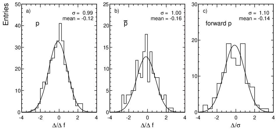
Another, independent cross check of the validity of the evaluation of the statistical errors is given by the two dimensional interpolation of the final cross sections described in Sect. 7. As this interpolation reduces the local statistical uncertainty by a factor of between 3 and 4, the deviations of the data points from the interpolated value in each bin should measure the real point by point statistical fluctuation. In fact the compatibility of the distribution of the relative deviations shown in Fig. 19 with an rms of unity confirms the correctness of the error estimate given above.
5.4 Estimation of K+ and contributions in the extreme forward direction
As the GTPC and VPC combination does not allow for particle identification via energy loss measurement, the proton extraction in the region 0.6, see in Fig. 8, has to rely on the measurement of /p and K+/p ratios from other experiments. In fact there are sufficient and mutually consistent data sets available to establish a reliable data base. The problem is alleviated by the fact that particle ratios are relatively stable against systematic errors of the different experiments and that their absolute values decrease rapidly to a few percent margin in the phase space region in question. The situation is shown in Fig. 12 in detail for /p, K+/p and (+K+)/p for different values as a function of transverse momentum. In both cases the ratios obtained by NA49 [1, 29] overlap consistently with the other data sets.

The interpolated lines shown in Fig. 12 have been used for the determination of proton cross sections from the total positive particle yields. The uncertainties connected with this procedure have been taken into account by an increase of the given statistical errors for the bins in question.
6 Evaluation of Invariant Cross Sections and Corrections
The experimental evaluation of the invariant cross section
| (7) |
follows the methods described in [1]. The normalization and the corrections are discussed below, concentrating on those issues specific for baryon measurements.
6.1 Empty target correction

The empty target background is treated as a correction factor as described in [1] by determining the baryon yields in the full and empty target samples and establishing their normalized difference relative to the full target sample. The resulting correction factor is shown in Fig. 13. It is, within the statistical errors, and independent and is compatible with the one given for pions [1]. The correction for neutrons is equal to the one for protons.
6.2 Trigger bias correction
The interaction trigger uses a circular scintillator of 2 cm diameter placed at a distance of 4 m from the target in anti-coincidence (S4 counter in Fig. 2). It accepts 89% of the total inelastic cross section. The majority of the vetoed events contain one fast proton in the small S4 acceptance. As explained in detail in [1] this event loss creates an and eventually dependent bias for the extracted data which has to be carefully examined as it depends on short range and long range correlations in the hadronic final state.
This trigger bias is determined by an off-line increase of the S4 radius. With this method the limiting value of each measured cross section at zero radius may be obtained. The S4 radius increase is possible as all tracks in the corresponding momentum region are detected via the GTPC+VPC+RCal combination (Sect. 3).

Figure 14 shows the size of the correction as a function of for protons and anti-protons. The results for two regions demonstrate that the correction is within errors independent of . Anti-protons exhibit a different dependence, again independent within the (larger) statistical errors in this case. The correction varies from the one for pions in the forward hemisphere due to the different correlation between leading protons and secondary baryons in the projectile fragmentation. For neutrons, the trigger bias correction is equal to the one for protons.
6.3 Re-interaction and absorption
The re-interaction of baryons in the hydrogen target has been evaluated, as in the case of pions [1], using the PYTHIA event generator. The corresponding corrections are shown in Fig. 15.

The absorption of baryons by interaction with the detector material has been elaborated based on the results for pions, modifying the absorption length in accordance with the higher baryonic interaction cross section.
6.4 Feed-down from weak decays
The determination of the contribution from weakly decaying baryons (, and their anti-particles) is based on the methods discussed in [1]. The parent particle input distributions are taken from published data and a subsequent Monte Carlo simulation is used to estimate the on-vertex reconstruction efficiency for baryonic daughters.
As the decay baryons are close in mass to the parent hyperons, they take up most of the parent momentum. Their distribution over the measured phase space is therefore much wider than the one for decay pions and extends over the complete and ranges. As shown in Fig. 16 this correction amounts to up to 15% for protons and 20% for anti-protons with dependences which are different for protons and anti-protons. For protons at large , where the contribution dominates the feed-down, it even increases at large .

The main systematic error source is the uncertainty of earlier measurements, especially for . For anti-protons, besides the also contributes for which there are no existing measurements. The yield of this particle was estimated from general anti-baryon/ baryon ratio and isospin arguments. To first order it was assumed that the and shapes are the same as for , and that the to ratio is 80% of the ratio. For neutrons the feed-down correction corresponds to the full relative yield from and decays, as shown in Fig. 16c.
6.5 Binning correction
The effect of finite bin sizes on the extracted inclusive cross sections was discussed in detail in [1] and shown to depend on the second derivative of the or distributions. Due to the approximately linear rather than exponential distribution of protons, the binning effects can in fact be neglected in longitudinal direction for the modest bin widths chosen. Also in transverse direction, due to the larger mean transverse momentum of baryons, the effect is smaller than for pions. As shown in Fig. 17 it reaches values in excess of 1% only at large due to the bin width of 0.2 GeV/c in this region.

6.6 Systematic errors
The systematic errors of the extracted cross sections are given by the normalization procedure and the uncertainties of the applied corrections. These contributions are estimated in Table 2. They are governed by the fluctuation of the detector absorption, feed-down and trigger bias corrections which are shown in Fig. 18 over all phase space bins, for protons and anti-protons.
| p | n | |||||
| Normalization | 1.5% | 1.5% | Normalization | 1.5% | ||
| Tracking efficiency | 0.5% | 0.5% | ||||
| Trigger bias | 0.5% | 1.0% | Trigger bias | 1% | ||
| Feed-down | 1.5% | 2.5% | Feed-down | 3% | ||
| Detector absorption | Detector absorption | |||||
| Target re-interaction | 0.5 – 1.5% | 1.0% | Target re-interaction | 0.5 – 1.5% | ||
| Binning correction | Binning correction | |||||
| Acceptance | 0 – 2% | |||||
| Energy scale error | 4 – 8% | |||||
| Energy resolution unfolding | 3 – 8% | |||||
| Charged veto efficiency | 2 – 3% | |||||
| Cluster overlap | 2% | |||||
| Hadron identification | 2 – 5% | |||||
| K contribution | 0 – 3% | |||||
| Total (upper limit) | 5.0% | 6.5% | Total (upper limit) | 28% | ||
| Total (quadratic sum) | 2.5% | 3.3% | Total (quadratic sum) | 10% |
With a linear sum of 5.0% and 6.5%, respectively, for protons and anti-protons, and quadratic sums of 2.5% and 3.3% they are only slightly larger than the ones estimated for pion production [1]. The larger systematic uncertainty of the neutron yields reflects the difficulties inherent in hadronic calorimetry as compared to charged track detection.

7 Results on double differential cross sections
7.1 Data tables
The binning scheme presented in Sect. 4 results in 333 and 143 data values for protons and anti-protons, respectively. These are presented in Tables 3 and 4.
| -0.05 | -0.025 | 0.0 | 0.025 | 0.05 | 0.075 | 0.1 | 0.125 | 0.15 | ||||||||||
| 0.1 | 2.349 | 2.76 | 2.161 | 1.90 | 2.121 | 1.78 | 2.128 | 1.75 | 2.224 | 1.69 | 2.340 | 1.76 | 2.620 | 1.83 | 3.039 | 1.55 | 3.479 | 1.76 |
| 0.2 | 2.158 | 3.53 | 1.921 | 1.60 | 1.837 | 1.46 | 1.854 | 1.42 | 1.901 | 1.44 | 2.095 | 1.49 | 2.349 | 1.50 | 2.666 | 1.36 | 2.998 | 1.49 |
| 0.3 | 1.664 | 3.72 | 1.570 | 2.63 | 1.631 | 1.81 | 1.575 | 1.41 | 1.664 | 1.26 | 1.750 | 1.31 | 1.935 | 1.33 | 2.179 | 1.34 | 2.549 | 1.28 |
| 0.4 | 1.297 | 4.24 | 1.286 | 2.74 | 1.287 | 2.26 | 1.238 | 1.71 | 1.334 | 1.37 | 1.379 | 1.43 | 1.486 | 1.52 | 1.742 | 1.49 | 1.880 | 1.52 |
| 0.5 | 1.094 | 3.96 | 0.951 | 3.25 | 0.977 | 2.45 | 0.929 | 1.98 | 0.973 | 1.47 | 1.057 | 1.45 | 1.161 | 1.52 | 1.224 | 1.56 | 1.353 | 1.72 |
| 0.6 | 0.707 | 4.38 | 0.689 | 3.62 | 0.645 | 3.24 | 0.688 | 2.46 | 0.712 | 1.98 | 0.709 | 1.78 | 0.807 | 1.67 | 0.884 | 1.74 | 0.948 | 1.91 |
| 0.7 | 0.493 | 5.38 | 0.451 | 4.31 | 0.449 | 4.07 | 0.494 | 2.76 | 0.482 | 2.47 | 0.533 | 2.15 | 0.526 | 1.93 | 0.601 | 1.78 | 0.654 | 2.11 |
| 0.8 | 0.378 | 6.13 | 0.357 | 5.10 | 0.314 | 4.45 | 0.322 | 3.52 | 0.329 | 3.19 | 0.3386 | 2.95 | 0.3686 | 2.42 | 0.3984 | 2.42 | 0.430 | 2.48 |
| 0.9 | 0.244 | 6.33 | 0.203 | 6.38 | 0.233 | 5.44 | 0.2196 | 4.49 | 0.2274 | 3.90 | 0.2399 | 3.46 | 0.2572 | 3.19 | 0.2503 | 3.33 | 0.2694 | 2.71 |
| 1.1 | 0.0956 | 4.75 | 0.0899 | 4.28 | 0.0927 | 3.14 | 0.0988 | 2.76 | 0.1078 | 2.42 | ||||||||
| 1.3 | 0.0445 | 7.71 | 0.0366 | 6.10 | 0.0384 | 4.67 | 0.0410 | 4.15 | 0.0398 | 3.64 | ||||||||
| 1.5 | 0.0199 | 9.72 | 0.0173 | 8.74 | 0.0188 | 6.90 | 0.0161 | 6.48 | 0.0163 | 6.46 | ||||||||
| 1.7 | 0.0087 | 14.2 | 0.00640 | 13.4 | 0.00617 | 11.3 | 0.00705 | 9.45 | 0.00607 | 9.60 | ||||||||
| 1.9 | 0.00284 | 14.3 | 0.00296 | 10.3 | ||||||||||||||
| 0.2 | 0.25 | 0.3 | 0.35 | 0.4 | 0.45 | 0.5 | 0.55 | 0.6 | ||||||||||
| 0.05 | 17.1 | 7.46 | 16.8 | 14.6 | ||||||||||||||
| 0.1 | 4.654 | 1.53 | 5.71 | 1.83 | 6.64 | 3.44 | 7.749 | 1.28 | 8.92 | 1.58 | 10.02 | 1.57 | 11.68 | 1.65 | 14.38 | 4.31 | 15.07 | 6.53 |
| 0.15 | 13.64 | 3.21 | 13.67 | 4.24 | ||||||||||||||
| 0.2 | 4.086 | 1.24 | 5.132 | 1.44 | 6.10 | 2.54 | 6.958 | 0.96 | 7.500 | 1.21 | 8.52 | 1.22 | 9.59 | 1.24 | 11.92 | 2.96 | 12.80 | 2.94 |
| 0.25 | 9.95 | 2.37 | 11.55 | 2.76 | ||||||||||||||
| 0.3 | 3.265 | 1.18 | 4.231 | 1.63 | 5.016 | 1.70 | 5.876 | 0.83 | 6.261 | 1.08 | 6.766 | 1.14 | 7.232 | 1.16 | 8.78 | 2.30 | 9.61 | 2.25 |
| 0.35 | 7.30 | 2.34 | 7.67 | 2.33 | ||||||||||||||
| 0.4 | 2.518 | 1.29 | 3.145 | 1.74 | 3.904 | 1.87 | 4.561 | 0.89 | 4.863 | 1.06 | 5.098 | 1.10 | 5.350 | 1.14 | 6.09 | 2.06 | 6.21 | 2.11 |
| 0.45 | 4.84 | 2.19 | 5.03 | 2.21 | ||||||||||||||
| 0.5 | 1.815 | 1.28 | 2.292 | 1.58 | 2.783 | 1.57 | 3.341 | 0.93 | 3.609 | 1.08 | 3.772 | 1.17 | 3.781 | 1.21 | 3.908 | 2.31 | 3.938 | 2.36 |
| 0.6 | 1.247 | 1.43 | 1.516 | 1.96 | 1.957 | 2.27 | 2.224 | 1.10 | 2.544 | 1.18 | 2.628 | 1.31 | 2.649 | 1.34 | 2.709 | 1.80 | 2.738 | 1.84 |
| 0.7 | 0.798 | 1.65 | 0.989 | 2.09 | 1.252 | 2.01 | 1.489 | 1.32 | 1.652 | 1.35 | 1.771 | 1.40 | 1.753 | 1.53 | 1.741 | 2.08 | 1.692 | 2.17 |
| 0.8 | 0.5092 | 1.71 | 0.620 | 1.94 | 0.756 | 2.35 | 0.894 | 1.59 | 1.021 | 1.61 | 1.140 | 1.61 | 1.127 | 1.71 | 1.128 | 2.43 | 1.028 | 2.61 |
| 0.9 | 0.3201 | 2.08 | 0.3672 | 2.38 | 0.458 | 2.63 | 0.548 | 1.92 | 0.605 | 1.94 | 0.676 | 1.97 | 0.689 | 2.11 | 0.672 | 2.91 | 0.614 | 3.12 |
| 1.1 | 0.1197 | 2.26 | 0.1388 | 2.42 | 0.1535 | 2.83 | 0.1657 | 2.22 | 0.1970 | 2.14 | 0.2071 | 2.25 | 0.2172 | 2.29 | 0.2124 | 3.43 | 0.1944 | 3.67 |
| 1.3 | 0.0439 | 3.72 | 0.0485 | 3.71 | 0.0527 | 4.54 | 0.0584 | 3.48 | 0.0587 | 3.63 | 0.0602 | 3.78 | 0.0629 | 3.94 | 0.0590 | 6.28 | 0.0567 | 6.57 |
| 1.5 | 0.0176 | 5.77 | 0.0156 | 6.43 | 0.0177 | 8.02 | 0.0207 | 5.42 | 0.0187 | 6.07 | 0.0182 | 6.38 | 0.0165 | 7.05 | 0.0153 | 11.4 | 0.0142 | 12.1 |
| 1.7 | 0.00578 | 8.75 | 0.00614 | 8.95 | 0.00628 | 9.37 | 0.00653 | 9.44 | 0.00709 | 9.45 | 0.00592 | 10.3 | 0.00549 | 17.8 | 0.0059 | 17.5 | 0.00235 | 27.6 |
| 1.9 | 0.00313 | 7.98 | 0.00245 | 10.6 | 0.00242 | 10.8 | 0.00161 | 21.2 | 0.00082 | 29.4 | ||||||||
| 0.65 | 0.7 | 0.75 | 0.8 | 0.85 | 0.9 | 0.95 | ||||||||||||
| 0.05 | ||||||||||||||||||
| 0.1 | 18.5 | 10.1 | ||||||||||||||||
| 0.15 | 14.09 | 5.64 | 14.0 | 9.72 | ||||||||||||||
| 0.2 | 12.68 | 3.88 | 14.74 | 4.94 | 15.0 | 8.35 | ||||||||||||
| 0.25 | 11.26 | 3.20 | 11.75 | 3.70 | 14.9 | 7.49 | 10.61 | 9.23 | ||||||||||
| 0.3 | 9.74 | 2.83 | 10.86 | 3.06 | 9.76 | 5.11 | 10.00 | 8.62 | 12.5 | 8.11 | ||||||||
| 0.35 | 8.09 | 2.34 | 7.34 | 3.09 | 7.93 | 3.42 | 8.48 | 4.52 | 10.18 | 4.94 | 12.39 | 7.76 | ||||||
| 0.4 | 6.55 | 2.42 | 6.19 | 2.58 | 6.47 | 3.53 | 6.46 | 3.67 | 7.71 | 4.64 | 9.00 | 5.07 | ||||||
| 0.45 | 5.13 | 2.24 | 5.03 | 2.70 | 4.93 | 2.82 | 5.08 | 3.20 | 5.43 | 3.91 | 6.78 | 4.80 | ||||||
| 0.5 | 4.028 | 2.41 | 3.930 | 2.52 | 3.752 | 2.65 | 4.05 | 2.63 | 3.55 | 3.36 | 4.98 | 3.21 | ||||||
| 0.6 | 2.592 | 1.95 | 2.507 | 2.04 | 2.322 | 2.18 | 2.247 | 2.28 | 2.238 | 2.35 | 2.464 | 2.28 | 4.954 | 1.81 | ||||
| 0.7 | 1.619 | 2.28 | 1.581 | 2.38 | 1.436 | 2.57 | 1.288 | 2.78 | 1.278 | 2.86 | 1.324 | 2.87 | 2.339 | 2.20 | ||||
| 0.8 | 0.984 | 2.75 | 0.973 | 2.84 | 0.886 | 3.06 | 0.768 | 3.35 | 0.686 | 3.66 | 0.711 | 3.68 | 1.130 | 2.97 | ||||
| 0.9 | 0.609 | 3.22 | 0.557 | 3.45 | 0.506 | 3.72 | 0.455 | 4.05 | 0.396 | 4.44 | 0.368 | 4.74 | 0.544 | 3.97 | ||||
| 1.1 | 0.1942 | 3.77 | 0.1757 | 4.07 | 0.1618 | 4.36 | 0.1334 | 4.92 | 0.1338 | 5.05 | 0.1185 | 5.50 | 0.1292 | 5.42 | ||||
| 1.3 | 0.0442 | 7.55 | 0.0392 | 8.24 | 0.0463 | 7.87 | 0.0350 | 9.24 | 0.0364 | 9.32 | 0.0404 | 9.08 | 0.0447 | 8.89 | ||||
| 1.5 | 0.0147 | 12.3 | 0.0136 | 13.0 | 0.0109 | 14.9 | 0.0084 | 17.4 | 0.0108 | 15.9 | 0.0131 | 14.8 | 0.0147 | 14.3 | ||||
| 1.7 | 0.00437 | 20.9 | 0.00421 | 22.1 | 0.00295 | 26.1 | 0.0045 | 22.4 | 0.00293 | 28.0 | 0.00379 | 25.9 | 0.0051 | 23.0 | ||||
| 1.9 | 0.00076 | 32.3 | 0.00119 | 28.4 | 0.00083 | 36.1 | ||||||||||||
| -0.05 | -0.025 | 0.0 | 0.025 | 0.05 | 0.075 | 0.1 | ||||||||
| 0.1 | 0.563 | 6.71 | 0.590 | 4.28 | 0.581 | 3.66 | 0.545 | 3.67 | 0.499 | 3.87 | 0.489 | 4.24 | 0.391 | 4.52 |
| 0.2 | 0.508 | 6.15 | 0.505 | 3.55 | 0.509 | 2.98 | 0.518 | 2.92 | 0.473 | 3.12 | 0.405 | 3.69 | 0.379 | 4.04 |
| 0.3 | 0.391 | 6.75 | 0.450 | 5.52 | 0.450 | 3.88 | 0.404 | 2.99 | 0.401 | 2.79 | 0.353 | 3.12 | 0.320 | 3.56 |
| 0.4 | 0.287 | 7.61 | 0.338 | 6.23 | 0.324 | 4.90 | 0.311 | 3.61 | 0.2848 | 3.17 | 0.2918 | 3.38 | 0.237 | 4.38 |
| 0.5 | 0.222 | 8.16 | 0.260 | 6.77 | 0.230 | 5.48 | 0.262 | 4.31 | 0.2324 | 3.22 | 0.2031 | 3.52 | 0.1761 | 4.38 |
| 0.6 | 0.163 | 8.52 | 0.178 | 8.99 | 0.178 | 6.67 | 0.1587 | 5.37 | 0.1511 | 4.82 | 0.1211 | 4.82 | 0.1255 | 4.72 |
| 0.7 | 0.117 | 9.82 | 0.103 | 10.4 | 0.1102 | 8.17 | 0.1168 | 6.29 | 0.1141 | 5.46 | 0.0929 | 5.56 | 0.0830 | 4.71 |
| 0.8 | 0.0534 | 15.7 | 0.0862 | 9.83 | 0.0845 | 8.84 | 0.0773 | 7.93 | 0.0637 | 7.22 | 0.0614 | 7.24 | 0.0600 | 6.58 |
| 0.9 | 0.0432 | 15.5 | 0.0427 | 13.9 | 0.0481 | 12.2 | 0.0409 | 10.7 | 0.0385 | 9.07 | 0.0441 | 8.11 | 0.0363 | 8.59 |
| 1.1 | 0.0155 | 12.3 | 0.0194 | 8.12 | 0.0153 | 7.39 | 0.0142 | 7.32 | ||||||
| 1.3 | 0.0095 | 14.7 | 0.00532 | 16.9 | 0.00515 | 13.3 | 0.00521 | 12.6 | ||||||
| 1.5 | 0.00272 | 27.1 | 0.00258 | 23.8 | 0.00241 | 20.2 | 0.00179 | 21.4 | ||||||
| 0.125 | 0.15 | 0.2 | 0.25 | 0.3 | 0.35 | 0.4 | ||||||||
| 0.1 | 0.355 | 4.98 | 0.260 | 7.36 | 0.194 | 7.09 | 0.115 | 11.5 | 0.074 | 18.1 | 0.0418 | 18.9 | 0.0173 | 55.1 |
| 0.2 | 0.300 | 4.49 | 0.275 | 5.57 | 0.183 | 7.15 | 0.0900 | 9.63 | 0.0613 | 14.4 | ||||
| 0.3 | 0.255 | 4.53 | 0.199 | 5.84 | 0.1654 | 4.69 | 0.0941 | 8.96 | 0.0429 | 14.7 | 0.0270 | 13.8 | 0.0137 | 29.5 |
| 0.4 | 0.203 | 4.98 | 0.165 | 6.14 | 0.1154 | 7.52 | 0.0645 | 10.5 | 0.0425 | 12.5 | ||||
| 0.5 | 0.1350 | 5.55 | 0.1231 | 5.73 | 0.0860 | 5.76 | 0.0463 | 10.3 | 0.0266 | 13.9 | 0.0161 | 13.6 | 0.0082 | 25.9 |
| 0.6 | 0.1005 | 6.69 | 0.0787 | 6.64 | 0.0578 | 8.62 | 0.0427 | 8.40 | 0.0190 | 14.9 | ||||
| 0.7 | 0.0705 | 5.72 | 0.0596 | 8.66 | 0.0443 | 9.05 | 0.0191 | 14.2 | 0.0162 | 14.7 | 0.0092 | 16.4 | 0.0062 | 21.8 |
| 0.8 | 0.0382 | 9.29 | 0.0346 | 10.8 | 0.0235 | 8.27 | 0.0151 | 14.8 | 0.0132 | 15.0 | ||||
| 0.9 | 0.0275 | 10.9 | 0.0242 | 10.0 | 0.0190 | 11.5 | 0.0141 | 11.7 | 0.0061 | 21.7 | 0.00435 | 20.6 | 0.00189 | 38.0 |
| 1.1 | 0.01008 | 9.15 | 0.00796 | 8.63 | 0.00447 | 16.1 | 0.00230 | 22.1 | 0.00182 | 27.0 | 0.00073 | 54.0 | ||
| 1.3 | 0.00403 | 15.5 | 0.00255 | 15.2 | 0.00152 | 21.7 | 0.00128 | 27.1 | ||||||
| 1.5 | 0.00127 | 22.8 | 0.00068 | 30.4 | 0.00057 | 34.5 | ||||||||
7.2 Extension of the data to high and low
As shown in Sect. 3 the NA49 detector acceptance is limited at large and low by the necessity of using an interaction trigger, vetoing through-going beam tracks. The corresponding acceptance gap extends from 0.05 at = 0.65 to 0.6 at = 0.95, see Fig. 1. In order to maintain the possibility of precise integration in this phase space region it is mandatory to use data from other experiments to supplement the NA49 results. Fortunately there are data from seven different experiments, all conducted at Fermilab in the years 1973 to 1982 [3, 4, 5, 6, 7, 8, 9] in exactly this region which also partially overlap with the NA49 data. These data come from internal target [3, 4, 5, 6] and bubble chamber experiments [7, 8], all performed in the target region at low proton lab momenta, and from a spectrometer experiment [9] in the forward hemisphere. If applicable the data have been transformed from the coordinate pair momentum transfer and missing mass into the and coordinates, interpolated to the values defined by the NA49 binning scheme and corrected for -dependence. This latter correction will be quantified in section 10 below. In total 123 data points are thus available as given in Table 5.
| ref | ref | ref | ref | ref | |||||||||||||||||||||||||
|---|---|---|---|---|---|---|---|---|---|---|---|---|---|---|---|---|---|---|---|---|---|---|---|---|---|---|---|---|---|
| = 0.6 | = 0.65 | = 0.7 | = 0.75 | = 0.8 | |||||||||||||||||||||||||
| 0.224 | 14 | .10 | 15 | .0 | 7 | 0.224 | 15 | .30 | 15 | .0 | 7 | 0.224 | 16 | .60 | 15 | .0 | 7 | 0.224 | 16 | .90 | 15 | .0 | 7 | 0.478 | 4 | .70 | 2 | .0 | 3 |
| 0.381 | 5 | .89 | 15 | .0 | 7 | 0.381 | 6 | .46 | 15 | .0 | 7 | 0.381 | 6 | .56 | 15 | .0 | 7 | 0.381 | 6 | .94 | 15 | .0 | 7 | 0.570 | 2 | .70 | 2 | .0 | 3 |
| 0.540 | 3 | .61 | 15 | .0 | 7 | 0.540 | 3 | .80 | 15 | .0 | 7 | 0.540 | 3 | .89 | 15 | .0 | 7 | 0.540 | 3 | .71 | 15 | .0 | 7 | ||||||
| 0.707 | 1 | .35 | 15 | .0 | 7 | 0.707 | 1 | .23 | 15 | .0 | 7 | 0.707 | 1 | .25 | 15 | .0 | 7 | 0.707 | 1 | .24 | 15 | .0 | 7 | 0.224 | 16 | .20 | 15 | .0 | 7 |
| 0.381 | 7 | .41 | 15 | .0 | 7 | ||||||||||||||||||||||||
| 0.200 | 13 | .34 | 3 | .3 | 9 | 0.300 | 10 | .45 | 2 | .0 | 9 | 0.540 | 3 | .52 | 15 | .0 | 7 | ||||||||||||
| 0.300 | 9 | .43 | 2 | .0 | 9 | 0.500 | 4 | .04 | 2 | .4 | 9 | 0.707 | 1 | .14 | 15 | .0 | 7 | ||||||||||||
| 0.400 | 6 | .31 | 2 | .6 | 9 | 0.750 | 1 | .32 | 4 | .4 | 9 | ||||||||||||||||||
| 0.500 | 4 | .14 | 2 | .3 | 9 | 0.500 | 4 | .06 | 1 | .0 | 9 | 0.300 | 11 | .67 | 1 | .4 | 9 | ||||||||||||
| 0.625 | 2 | .42 | 2 | .7 | 9 | 0.750 | 1 | .26 | 1 | .6 | 9 | 0.500 | 4 | .10 | 1 | .5 | 9 | ||||||||||||
| 0.750 | 1 | .41 | 3 | .3 | 9 | 0.750 | 1 | .00 | 2 | .9 | 9 | ||||||||||||||||||
| 0.300 | 8 | .82 | 5 | .4 | 9 | 0.500 | 3 | .90 | 1 | .3 | 9 | ||||||||||||||||||
| 0.400 | 5 | .93 | 1 | .0 | 9 | 0.750 | 1 | .00 | 2 | .0 | 9 | ||||||||||||||||||
| 0.500 | 4 | .03 | 1 | .6 | 9 | ||||||||||||||||||||||||
| 0.625 | 2 | .40 | 1 | .2 | 9 | ||||||||||||||||||||||||
| 0.750 | 1 | .41 | 1 | .0 | 9 | ||||||||||||||||||||||||
| = 0.85 | = 0.9 | = 0.95 | = 0.975 | ||||||||||||||||||||||||||
| 0.511 | 4 | .18 | 2 | .0 | 3 | 0.537 | 3 | .91 | 2 | .0 | 3 | 0.182 | 34 | .10 | 5 | .0 | 4 | 0.188 | 44 | .51 | 5 | .0 | 4 | ||||||
| 0.602 | 2 | .33 | 2 | .0 | 3 | 0.629 | 2 | .12 | 2 | .0 | 3 | 0.246 | 23 | .35 | 5 | .0 | 4 | 0.253 | 31 | .24 | 5 | .0 | 4 | ||||||
| 0.299 | 21 | .15 | 5 | .0 | 4 | 0.302 | 30 | .31 | 5 | .0 | 4 | ||||||||||||||||||
| 0.190 | 20 | .83 | 5 | .0 | 4 | 0.157 | 28 | .41 | 5 | .0 | 4 | 0.337 | 18 | .94 | 5 | .0 | 4 | 0.344 | 28 | .09 | 5 | .0 | 4 | ||||||
| 0.245 | 16 | .73 | 5 | .0 | 4 | 0.225 | 20 | .83 | 5 | .0 | 4 | 0.375 | 14 | .52 | 5 | .0 | 4 | 0.384 | 21 | .79 | 5 | .0 | 4 | ||||||
| 0.290 | 15 | .47 | 5 | .0 | 4 | 0.275 | 17 | .68 | 5 | .0 | 4 | 0.409 | 12 | .15 | 5 | .0 | 4 | 0.416 | 20 | .20 | 5 | .0 | 4 | ||||||
| 0.328 | 12 | .00 | 5 | .0 | 4 | 0.318 | 16 | .10 | 5 | .0 | 4 | ||||||||||||||||||
| 0.363 | 9 | .63 | 5 | .0 | 4 | 0.355 | 12 | .31 | 5 | .0 | 4 | 0.224 | 33 | .30 | 15 | .0 | 7 | 0.224 | 53 | .20 | 15 | .0 | 7 | ||||||
| 0.389 | 10 | .10 | 5 | .0 | 4 | 0.381 | 14 | .44 | 15 | .0 | 7 | 0.381 | 25 | .18 | 15 | .0 | 7 | ||||||||||||
| 0.224 | 17 | .20 | 15 | .0 | 7 | 0.540 | 6 | .84 | 15 | .0 | 7 | 0.540 | 12 | .16 | 15 | .0 | 7 | ||||||||||||
| 0.381 | 7 | .80 | 15 | .0 | 7 | 0.224 | 21 | .40 | 15 | .0 | 7 | 0.707 | 1 | .60 | 15 | .0 | 7 | 0.707 | 3 | .14 | 15 | .0 | 7 | ||||||
| 0.540 | 3 | .32 | 15 | .0 | 7 | 0.381 | 9 | .12 | 15 | .0 | 7 | ||||||||||||||||||
| 0.707 | 1 | .05 | 15 | .0 | 7 | 0.540 | 3 | .52 | 15 | .0 | 7 | 0.179 | 43 | .10 | 2 | .0 | 5 | 0.186 | 69 | .80 | 2 | .0 | 5 | ||||||
| 0.707 | 1 | .06 | 15 | .0 | 7 | 0.263 | 24 | .20 | 2 | .0 | 5 | 0.269 | 41 | .30 | 2 | .0 | 5 | ||||||||||||
| 0.210 | 16 | .70 | 5 | .0 | 5 | 0.350 | 17 | .90 | 2 | .0 | 5 | 0.357 | 30 | .20 | 2 | .0 | 5 | ||||||||||||
| 0.302 | 11 | .80 | 5 | .0 | 5 | 0.154 | 29 | .50 | 6 | .0 | 5 | 0.430 | 11 | .00 | 2 | .0 | 5 | 0.438 | 19 | .70 | 2 | .0 | 5 | ||||||
| 0.384 | 7 | .47 | 5 | .0 | 5 | 0.244 | 17 | .70 | 6 | .0 | 5 | ||||||||||||||||||
| 0.330 | 12 | .80 | 4 | .0 | 5 | 0.110 | 41 | .30 | 5 | .9 | 6 | 0.119 | 58 | .20 | 5 | .0 | 6 | ||||||||||||
| 0.410 | 7 | .87 | 4 | .0 | 5 | 0.212 | 30 | .20 | 5 | .8 | 6 | 0.220 | 49 | .10 | 4 | .0 | 6 | ||||||||||||
| 0.190 | 25 | .70 | 4 | .0 | 6 | 0.160 | 46 | .23 | 15 | .0 | 8 | 0.160 | 67 | .60 | 15 | .0 | 8 | ||||||||||||
| 0.316 | 19 | .50 | 15 | .0 | 8 | 0.316 | 42 | .65 | 15 | .0 | 8 | ||||||||||||||||||
| 0.160 | 29 | .17 | 15 | .0 | 8 | 0.447 | 10 | .07 | 15 | .0 | 8 | 0.447 | 14 | .79 | 15 | .0 | 8 | ||||||||||||
| 0.316 | 14 | .96 | 15 | .0 | 8 | 0.548 | 7 | .24 | 15 | .0 | 8 | 0.548 | 10 | .47 | 15 | .0 | 8 | ||||||||||||
| 0.447 | 7 | .32 | 15 | .0 | 8 | 0.632 | 4 | .07 | 15 | .0 | 8 | 0.632 | 6 | .03 | 15 | .0 | 8 | ||||||||||||
| 0.548 | 5 | .01 | 15 | .0 | 8 | ||||||||||||||||||||||||
| 0.632 | 2 | .72 | 15 | .0 | 8 | ||||||||||||||||||||||||
| 0.500 | 4 | .55 | 1 | .1 | 9 | ||||||||||||||||||||||||
| 0.750 | 1 | .01 | 1 | .0 | 9 | ||||||||||||||||||||||||
The data are well consistent within their statistical errors, both between the different experiments and with the NA49 results in the overlap region. The only exception is given by the bubble chamber experiment [8] where at below 0.9 the cross sections deviate from all other experiments by +20% to +30% independent of . This difference cannot be understood by eventual mis-identification nor by binning effects. Data from [8] are therefore only used at 0.9.
7.3 Interpolation scheme
As in the preceding publications concerning pions [1, 30] a two-dimensional interpolation is applied to the data which reduces the local statistical fluctuations given by the errors of the data points by a factor of 3-4. As there is no possibility to describe the detailed and distributions by simple functions and as any algebraic approximation risks to dilute the data quality by introducing systematic biases, the interpolation scheme relies on a multi-step recursive method using eyeball fits. The quality of this procedure may be controlled by plotting the differences between data points and interpolation, normalized to the statistical errors. The resulting distribution should be a Gaussian centered at zero with variance unity. This is demonstrated in Fig. 19 for protons and anti-protons as far as the NA49 data points are concerned, and separately for the extension to higher at low described above.
As, in this latter region, there are practically no measurements below = 0.2-0.3 GeV/c the extrapolation to = 0 has to be independently quantified. In this limited range of transverse momentum and at 0.6 a parametrization of the form
| (8) |
with has been applied. The parameters and are shown in Fig. 20 as a function of .

The slope extrapolates well to the value for low- elastic scattering at SPS energy also shown in Fig. 20
The internal consistency of the data sets used and their compatibility with the interpolation scheme as well as with the extrapolation to very low is presented in Fig. 21.

It should be noted that the measured cross sections deviate rapidly from the low- parametrization, Eq. 8, already at values of 0.4 GeV/c. This is exemplified by the dashed lines in Fig. 21 for two values. Fits over larger regions of therefore result systematically in smaller values of [8], see also the discussion in Sect. 12.
7.4 Dependence of the invariant cross sections on and


The shape of the invariant cross section as functions of and is shown in Figs. 22 and 23. These Figures include the data interpolation discussed above. In order to clearly demonstrate the shape evolution and to avoid the overlap of the interpolated curves and of the error bars, subsequent distributions have been multiplied by factors of 0.5 (Fig. 22).
7.5 /p ratios

The phase space distributions of protons and anti-protons are rather similar in transverse momentum, Fig. 22, but they show important differences in longitudinal momentum, Fig. 23. Here the invariant proton cross sections increase with whereas the anti-protons fall off steeply with similar to mesonic production [1]. It is therefore interesting to scrutinize the /p ratios quantitatively in both co-ordinates. This is presented in Fig. 24 which shows this ratio as a function of for fixed (left panels) and as a function of for fixed (right panel). In all plots the results from the two-dimensional interpolation discussed above are shown as lines through the data points.
Several features emerge from this comparison. The /p ratio falls with increasing at 0.1 and increases with at 0.15. The ratio between = 0.1 and = 1.5 GeV/c is about 2 at low and about 0.5 at high . This means that the distribution of the anti-protons flattens out with increasing until it becomes significantly broader than the one for protons at 0.3.
The /p ratio as a function of at fixed also shows distinctive trends. Here the steep dependence at low (a factor of about 130 between = 0 and = 0.4) flattens out at higher (a factor of only 30 over the same range).
The situation is clarified by the summary plots of Fig. 25 where only the interpolated lines are shown as functions of and , respectively.

7.6 Rapidity and transverse mass distributions

As in references [1, 30] the invariant cross sections are also presented, for convenience, as a function of rapidity at fixed in Fig. 26. Here the absence of a ”rapidity plateau” both for protons (with the exception of the region at 1.5 GeV/c) and for anti-protons should be noted.

Transverse mass distributions, with = , are shown in Fig. 27 for = = 0. In accordance with the /p ratios discussed above, a systematic difference between p and is visible. The proton distribution is clearly not compatible with simple exponential shape, whereas the anti-proton distribution happens to be close to exponential up to the experimental limit of = 0.8 GeV/c2.This is quantified by the dependence of the local logarithmic inverse slopes of given in Fig. 28. Here the slope defined by three successive data points has been used. In Fig. 28 also the inverse slopes obtained from the data interpolation, Sect. 7.3, are shown.

7.7 Baryon to pion ratios
The NA49 data on charged pions [1] offer a phase space coverage which is comparable in completeness, density and statistical accuracy to the results on baryons presented here. It is therefore indicated to compare the respective cross sections. This is done in the following section by inspecting the corresponding ratios of invariant inclusive cross sections as functions of and .
For protons, the ratio , where indicates the mean pion cross section , is presented in Fig. 29a as a function of at fixed and in Fig. 29b as a function of for fixed . For each data sample the corresponding interpolated cross section ratios are superimposed as full lines.

The dependence, Fig. 29a, reveals structure at low which has been shown in [1] to result from resonance decay, together with a strong increase of the ratio by almost three orders of magnitude between = 0 and = 0.5. This increase is progressively reduced with increasing to less than an order of magnitude at 2 GeV/c. In fact approaches unity in the high region for all values shown, and the extrapolation of the data interpolation (full lines) beyond the measured range indicates a convergence point at 1 for 2.5 GeV/c. This is again an indication of resonance decay. A study of the pion cross sections resulting from the decay of an ensemble of 13 known resonances [42, 44] has indeed shown that the inclusive pion yields are saturated in the range 1.5 3 GeV/c, at SPS energy, by two-body resonance decays. The high pions originate either from high mass resonances or from the high mass Breit-Wigner tails of lower mass states. In both cases the available momentum in the resonance cms becomes high enough so that the dependence on the mass of the decay particle induced by the energy term
| (9) |
in the Lorentz-transformation from the resonance cms to the experimental system becomes small. This means, always considering two-body decays, that the yield dependence on the kinematical variables and should become similar for pions and protons and therefore their ratio should tend to be stable against these variables. The actual limiting value of p/ depends however on the details of the isospin structure of the baryonic and mesonic resonances contributing to the proton and pion production in this section of phase space [42, 44].
The dependence at fixed , Fig. 29b, shows again the strong increase of with in the low region, with a progressive tendency to flatten out with increasing . This results, at up to about 1 GeV/c, in a convergence point at 0.5 where becomes practically independent predicting the equality of mean for pions and protons in this region shown in Sect. 10.1, Fig. 56. At 1.1 GeV/c and 0.3, see Fig. 29c, the distribution of protons becomes steeper than the one for pions. The ratio thus approaches unity from above, whereas at 0.3, Fig. 29b, the opposite trend is visible as discussed above.
Concerning the relation of anti-protons to pions it is indicated to rather study the / ratios. This is due to the similar isotriplet structure of both the baryon-pair and the pion production [33], see also Sect. 11.1. The / ratios are shown in Fig. 30 both as a function of at fixed and as a function of at fixed .

Due to the larger error bars for production together with the smaller range of variation, data points and interpolated lines of subsequent (Fig. 30a) and (Fig. 30b) values are shifted upwards by 0.02 in /. The full lines correspond again to the two-dimensional interpolation of the invariant cross sections.
Similar to what has been shown for p/, the / ratios increase strongly with at low by about one order of magnitude, Fig. 30a. And similarly, this increase reduces for larger to a factor of only 2 at the limit of the measurements at = 0.35. In contrast there is a general flattening of the dependence for beyond about 1.2 GeV/c.
As far as the dependence is concerned, Fig. 30b, the strong increase observed for p/ with is inverted to a general modest decrease which amounts to a factor of about four between = 0 and 0.35 at the highest values. At below 0.4 GeV/c however the ratios show a distinct maximum at 0.2 and little if any difference comparing the values at = 0 and 0.35.
In order to bring out the trends described above more clearly, the ratios of the interpolated cross sections are shown, without scale shift, separately in Figs. 31a and 31b.

Here again, it is worth to note the flattening of the dependence above 1.2 GeV/c and the convergence of the ratios for the higher range where the mean for and pions becomes comparable.
8 Comparison to Fermilab data
8.1 The feed-down problem
Before proceeding to a detailed comparison with the data sets specified in Sect. 2, the general problem of baryon feed-down from weak decays of strange hyperons has to be discussed. In the case of the NA49 data a feed-down correction has been performed (Sect. 6.4). It amounts to typically 5-20% of the measured baryon yields, with specific and dependences. This is only a fraction of the total hyperon decay contribution as the TPC tracking system of the NA49 detector has a resolution of the primary vertex position sufficient to reject a major part of the decay baryons. This is not a priori true for the reference data. As most of the corresponding experiments date from the 1970’s to the early 1980’s, micro-vertex detection or precision tracking was not available and therefore a large fraction if not all of the decay baryons contributed to the measured cross sections. What counts here is the distance of the first tracking elements from the primary vertex in relation to the typical hyperon decay length.
For the CERN ISR collider it may be stated that, given the different detector layouts for the and ranges covered, and given the large dimension of the interaction diamond, practically all baryonic decay products are included in the published data. A correction for this feed-down has not been attempted by any of the quoted experiments.
For fixed-target experiments the situation is somewhat more complicated as the range of lab momenta covered shows a much larger variation. Measurements in the target hemisphere with lab momenta comparable to the range at colliders are definitely prone to feed-down contamination. But even in the forward direction with momenta in the range of several tens of GeV/c, in many cases the first active detector elements are many meters away from the primary vertex, not to mention the general absence of precision tracking. A precise simulation of trajectories through the detectors and the aperture-defining collimators would be mandatory to come to a quantitative determination of the feed-down contributions.
A feeling for the size of the corresponding corrections may be obtained from Fig. 32 where the total yield of decay products is given in percent of the direct baryon cross section for protons and anti-protons at = 17.2 GeV/c.

Whereas this fraction tends to decrease below the 10% level at 0.4 for protons, it stays constant or even increases with for anti-protons, with a sizeable dependence. The data comparisons carried on below will therefore attempt to address this problem on a case-to-case basis.
8.2 The Brenner et al. data, [9]

This experiment offers 90 overlapping data points for protons and 19 points for anti-protons at the two beam momenta of 100 and 175 GeV/c. If the statistical errors of the proton sample are typically on the 1-10% level, the ones for anti-protons are considerably larger and vary between 20 and 50%. The situation is quantified in Fig. 33 which shows the distributions of the statistical errors, the differences to the interpolated NA49 data and the differences normalized to the statistical errors for protons and anti-protons, with and without feed-down correction of [9]. This latter distribution should be centered at zero with variance unity if the two measurements are compatible on an absolute scale.
Evidently the feed-down correction helps to reduce the almost 50% average difference for anti-protons, but over-corrects for protons. It should however be realized that the mean differences are for protons on the 4% level which signals good agreement if compared to the quoted absolute normalization errors. This result verifies the excellent agreement found in [1] for pions.
The distribution of the comparison data over phase space may be judged from Fig. 34 where the and distributions of the data points from [9] are given against the interpolated NA49 data.

8.3 The Johnson et al. data, [10]
From this experiment 54 and 26 data points for protons and anti-protons, respectively, may be used for comparison. The data were obtained at 100, 200 and 400 GeV/c beam momentum. As in the Brenner experiment, there is a large difference between the statistical errors of protons (2-6%) and anti-protons (10-30%).
As the measurements were done in the backward hemisphere up to maximum lab momenta of 2.3 GeV/c and as the aperture defining first magnet is placed at about 7 decay lengths for the maximum contributing hyperon momentum, a major fraction of the feed-down baryons must be expected to be contained in the data sample. This is visible in Fig. 35 where again the distributions of the statistical error, of the difference and the relative difference to the NA49 data with and without feed-down correction are presented.

Particularly for protons an improvement of the experimental differences is visible with feed-down correction, with mean deviations on the few percent level. The large rms values of the relative differences are, however, noteworthy. As was already the case for the pion comparison [1], this speaks for additional fluctuations beyond those from counting statistics proper in this experiment. Why the mean relative deviations are below one standard deviation for the baryons and about 3 standard deviations for pions [1] remains however an open question.
The phase space distribution of the Johnson data, compared to the NA49 data interpolation, is shown in Fig. 36.

8.4 The Antreasyan et al. data, [2]
This so-called ”Cronin” experiment represents the only measurement near = 0 in the SPS energy range. As it is overlapping with the lower ISR energy range there is a long standing problem with an unresolved discrepancy of the proton yields by about a factor of 1.3–1.4 and of the anti-proton yields by a factor of 2, whereas there is reasonable agreement of the pion cross sections [18]. The experiment which was aiming at high production contributes just a couple of cross sections at the values of 0.77 and 1.54 GeV/c in the NA49 range.
A first problem is connected with the fact that the spectrometer was set to a constant lab angle of 77 mrad at all energies and for all particle masses. This results in an and dependent offset in which introduces non-negligible variations of the cross sections. This is quantified in Table 6 which gives the corresponding deviations in and of proton and anti-proton cross sections , referred to = 0.
| 200 | 300 | 400 | |||||
|---|---|---|---|---|---|---|---|
| 19.3 | 23.7 | 27.3 | |||||
| 0.77 | -0.0 | 28 | -0.0 | 45 | -0.0 | 53 | |
| [%] | -3 | .5 | -8 | .9 | -12 | .0 | |
| [%] | 1 | .2 | 3 | .1 | 4 | .2 | |
| 0.713 | 0.081 | 0.972 | 0.097 | 0.956 | 0.101 | ||
| 0.726 | 0.084 | 0.797 | 0.082 | 0.760 | 0.081 | ||
| 1.54 | 0.0 | 13 | -0.0 | 20 | -0.0 | 37 | |
| [%] | -0 | .3 | -0 | .8 | -2 | .2 | |
| [%] | – | – | – | ||||
| 0.756 | 0.058 | 1.230 | 0.059 | 1.540 | 0.059 | ||
| 0.728 | 0.044 | 0.824 | 0.044 | 0.809 | 0.074 | ||
A second problem is also here connected to feed-down. As the first, aperture-defining collimators of the spectrometer are about 18 m downstream of the target, a good fraction of the feed-down baryons may enter into the acceptance. Following Fig. 32 this may well give downward corrections of up to 18% for protons and 13 to 16% for anti-protons in the given range.

The cross section ratios between the data from [2] and NA49 are also presented in Table 6. They are shown in Fig. 37a for protons and Fig. 37b for anti-protons as a function of . For protons there is to first order an -independent offset at 0.75, whereas for anti-protons the expected strong -dependence of anti-baryon production is evident. In this case however, when extrapolating this dependence to = 17.2 GeV, there is a discrepancy of about a factor of two as compared to the NA49 data. Similar discrepancies have been mentioned above with respect to the ISR data.
In order to clarify this experimental situation one may take reference to data at lower and at ISR energies. In Table 7 the cross section ratios between the PS experiment of [31] at = 4.9 and 6.8 GeV, the Serpukhov experiment of [32] at = 11.5 GeV and the ISR measurements [18, 19] at = 23 and 31 GeV, and NA49 are given. These data ratios are presented in Fig. 38 as a function of .
| / | 4.9 | 6.8 | 11.5 | 23.0 | 31.0 | ||||||
|---|---|---|---|---|---|---|---|---|---|---|---|
| 0.77 | 0.338 | 0.05 | 1.34 | 0.15 | 1.68 | 0.22 | |||||
| 3.13 | 0.30 | 1.99 | 0.22 | 1.37 | 0.18 | 1.02 | 0.10 | 1.07 | 0.10 | ||
| 1.54 | 0.270 | 0.05 | 2.40 | 0.40 | 3.50 | 0.60 | |||||
| 2.35 | 0.60 | 1.76 | 0.60 | 0.970 | 0.15 | 0.992 | 0.15 | 1.13 | 0.15 | ||

In Fig. 38a the very strong decrease of the central invariant proton cross section up to SPS energies is evident. This decrease is compensated by the comparatively strong increase of pair produced protons from Serpukhov through SPS up to ISR energies which produces an effective flattening of the -dependence between = 17.2 and 31 GeV followed by a steady increase at higher energies. As explained in detail in [33] the proper subtraction of the yield of pair-produced protons results in a continued decrease of the net proton yield to about zero at the highest ISR energies.
As shown in Fig. 38b the increase of the anti-proton cross sections from threshold through Serpukhov and SPS to ISR energies gives a consistent picture in the comparison of the experiments quoted in Table 7. The difference in the -dependence between the lower range at 0.77 GeV/c and the of 1.54 GeV/c should be noted. It is evident also in the Cronin data, Fig. 37b.
In conclusion it appears that the data from [2] seem to be low for baryons in comparison to all other available data, by 25% for protons and 50% for anti-protons.
9 Comparison to ISR and RHIC data
As shown in Fig. 1 the ISR data on baryons cover the / plane quite extensively with a series of different spectrometer experiments in the range of from 23 to 63 GeV. The present paper will limit the detailed comparison to the forward region at 0.1, with the exception of the preceding chapter where a few points at = 0 were included in order to clarify the experimental situation. The reason for this limitation lies in the rapid evolution of both the proton and anti-proton yields at central rapidity and in the difficulties of defining ”net” protons as the difference between proton and pair-produced proton cross sections. Here, the use of data from the isospin-reflected reaction n+p p, is mandatory in order to fully understand the isospin structure of baryon pair production [33]. The central area will therefore be treated in a subsequent publication including the neutron beam data available to NA49.
The main interest in regarding the forward ISR region of baryon production lies in a detailed study of -dependence both of the proton and anti-proton cross sections, especially in relation to scaling concepts and to the question of form stability of the and distributions. Two collaborations [11, 12, 13, 14, 15, 16, 17] have contributed data in forward direction, with more than 1200 data points for protons and a comparatively rather limited set of only about 100 points for anti-protons.
It should be remarked that all ISR data are corrected by us for baryon feed-down from hyperon decay as described in Sect. 8.1.
9.1 Proton data [12, 13, 14] from ISR
The rich data set of [12, 13, 14], if compared directly and as a whole to the NA49 data, reveals a discouragingly wide distribution of differences, Fig. 39, with an rms of twice the mean statistical error and a full width at base of more than 50%. It will be demonstrated below that this may be understood as the combination of two effects, namely an apparent normalization uncertainty of about 10% rms and a very sizeable shape change of the distributions in the region 0.7 which introduces systematic deviations of up to 30%. In order to bring this out clearly the comparison will be conducted in several steps.


A first step regards the data [12] at = 31 GeV (118 points), covering a range from 0.5 to 1 in and from 0.47 to 1.08 GeV/c in . The necessary feed-down correction to these data is relatively small, ranging from 8% at the lowest to zero for 0.85. The overall distribution of differences against NA49 is shown in Fig. 40a where again the large width and a considerable offset are evident. When however plotting the differences for each of the 25 available values separately, Fig. 40b, a sizeable depletion of the ISR data above = 0.7 becomes visible, followed by a rapid increase towards the diffractive peak at 0.97. The mean values over at each , Fig. 40c, indicate this trend with good precision. When plotting the point-by-point differences to this curve, Fig. 40d, the rms width is reduced to the expected mean value of the statistical errors.
It should be pointed out that in the region below = 0.7 the mean difference is flat and close to zero with an offset of about +2.5% with respect to the NA49 data. This is a first indication of approximate scaling.
In a second step the data [13] are compared to NA49. This data set (134 points) covers a wide range from 0.17 to about 2 GeV/c with ranging from 0.3 to 0.7. These data are therefore below the region of depletion discussed above. The ranges from 31 to 53 GeV.
A first look at the 9 available distributions at the different and values as compared to the interpolated NA49 data, Fig. 41, shows good agreement as far as the shape over the full range of is concerned.

There are however noticeable offsets with respect to NA49 which may be described by multiplicative factors as shown in Table 8.
| / | 31 | 45 | 53 |
|---|---|---|---|
| 0.3 | 1.00 | ||
| 0.4 | 0.83 | ||
| 0.5 | 1.05 | ||
| 0.6 | 1.09 | 1.18 | 1.18 |
| 0.7 | 1.05 | 1.33 | 1.33 |
Applying these factors to the ISR data the distribution of differences to NA49 becomes centered at zero with a variance which corresponds to the mean of the given statistical errors, Fig. 42.

The mean of the offset factors, including the first data set discussed above, amounts to 1.10. This might indicate a general increase of the proton cross sections at ISR energies compared to the SPS by this amount. The sizeable fluctuation of the offset with both and shown in Table 8 indicates however at least an additional normalization problem.
This problem can be quantified in a third step by comparing the large data set [14] with about 1000 data points spread over 9 different values of from 23 to 62 GeV, with and ranges of 0.3–1.7 GeV/c and 0.64–0.96, respectively. It should be mentioned that this experiment did not have particle identification so that in the lower range a correction for and had to be applied (see Sect. 5.4).
A first impression of the evolution of the invariant cross section in the region above = 0.65 may be obtained from Fig. 43 which shows the averaged deviations from the NA49 data as a function of for the nine values. Although the depletion at 0.8 is generally similar to the one shown at = 31 GeV (Fig. 40c) rather important overall deviations from unity in the flat region below = 0.7 are visible, similar to the ones given in Table 8 for = 45 GeV.

Tentatively normalizing this lower region to the NA49 data one obtains the normalization factors given in Fig. 44 as a function of ,including also the ones from Table 8. The projection of this distribution on the vertical axis shows a wide spread with an rms of about 14% and a mean of 1.16.

The variance is in agreement with the normalization uncertainty given by the experiment. The offset might indicate a general increase of the invariant cross section over the ISR energy range by about this amount. This will be discussed in more detail below.
As visible from Fig. 43 the depletion at high develops in a characteristic fashion as a function of . In order to bring this evolution out more clearly the ISR data are normalized to NA49 using the low- correction factors of Fig. 44 and the mean ratios plotted as a function of at fixed in Fig. 45.

In this Figure, the data from [3] have been included. Their slope against has been used in Sect. 7.2 to correct the high- Fermilab data for -dependence. As is visible from Fig. 45 a consistent, smooth decrease of the invariant cross sections from = 8 to = 63 GeV/c is experimentally established. It continues to lower with the data from [31] not shown here. Seen as a function of this decrease starts at 0.75 with a few percent depletion and reaches its maximum at 0.90–0.95 with an almost 40% effect.
In this context it is of course interesting to look at the higher range of the p+ colliders. Only one data set from the UA4 experiment [34] is available here which covers the range from 0.92 to 1 with four values between 0.74 and 1.07 GeV/c. Applying the same method described above by averaging over and normalizing to the NA49 data, the dependence shown in Fig. 46 is obtained.

Although the compatibility of the UA4 data with ISR results has been noted in [34] the strong -dependence from lower energies implies a minimum of the invariant cross section at about RHIC energy and a subsequent rise towards p+ collider energy, Fig. 46. This raises another question concerning baryon number conservation. As the total inelastic cross section rises by 13% at the highest ISR energy and by 48% at = 540 GeV as compared to SPS energies, the proton density at high will decrease faster than the invariant cross section with increasing . This is indicated by the dashed line in Fig. 46 which shows the evolution of proton density rather than invariant cross section. In this case a flattening of the -dependence up to collider energy is not excluded. As at the same time the central net proton density decreases at the higher ISR energy range [33] the eventual scaling of the invariant cross section in the intermediate range has to be questioned. Unless the whole decrease of proton density at low and high plus the increase of the inelastic cross section is absorbed into increased neutron or heavy flavour (mostly strangeness) production, there should be problems with baryon number conservation. In this sense the mean increase by about 20% of the invariant proton cross section which is visible in the average cross section ratios of Fig. 44 might be real. In fact the percentage rise of the inelastic cross section over the ISR energy range is also indicated in this Figure. Although of course the large systematic uncertainties in the ISR data do not allow for a definite statement, an upwards scaling violation of the invariant proton cross section of 10-20% over the ISR region cannot be excluded at this stage. The interesting intermediate region at RHIC energy is only covered in the interval 0.1 0.3 by the BRAHMS experiment [43] in two rapidity windows, see Sect. 9.5. However, recent data from deep inelastic leptoproduction at HERA [38, 39] help to fill the gap in up to the kinematic limit at 130 GeV, see Sect. 12.
9.2 Proton data [17] from ISR
The data of Capiluppi et al. [17] offer an additional set of proton cross sections with 184 points at four ISR energies and and ranges of 0.16–1.38 GeV/c and 0.05–0.6 respectively. This coverage has some overlap with the data [12, 13, 14] discussed above.
Plotting again, after feed-down correction, the point-by-point differences to the NA49 data, Fig. 47, a picture similar to Fig. 39 emerges with an average offset of +6% and an rms of 17%.

Given a mean statistical error of the data [17] of 13%, Fig. 48, this variance indicates again additional normalization and/or and dependences which are however much smaller than the ones found in the forward data of [12, 13, 14]. The distributions of the differences with respect to the NA49 data plotted separately for the four values, Fig. 48, indicate only a small if any s-dependence. There is also, within the statistical uncertainties, no discernible dependence as shown by the mean differences as a function of in Fig. 48.

It should however be mentioned that in this region there are two counteracting phenomena to be taken into account. Firstly there is the decrease of central net proton density with increasing in the approach to baryon transparency [33]. Secondly there is the strong increase of pair produced protons with , see Sect. 9.3 below. Both phenomena extend over the region of studied here. A detailed discussion has to take into account, as already mentioned in Sect. 8.4 above, the isospin structure of baryon pair production. This will be elaborated in a subsequent publication. The observed overall offset of about +6% indicates again a possible upwards scaling violation of the invariant cross section in the ISR energy range on the 10% level.
9.3 Anti-proton data [15, 16] from ISR
The data of Albrow et al. [16] have been obtained at fixed angle and for three ISR energies of 31, 45 and 53 GeV. They cover a range of 0.12 to 0.6 in and 0.16 to 0.8 GeV/c in . The comparison to the NA49 data is shown in Fig. 49a without and 49b with feed-down subtraction.

The difference distributions of Fig. 49 show an offset of 34% for the non-subtracted case which reduces to 2% applying the feed-down correction. The variance of the distributions is again somewhat larger than the mean statistical error of 17% necessitating an additional fluctuation of the normalization of about 13% rms which complies with the estimated margin. There is no discernible -dependence in the ISR data itself, and no -dependence up from SPS energy after feed-down subtraction. This somewhat surprising result is verified by the second measurement [15] which provides 14 data points at fixed = 0.19 and ranging from 0.14 to 0.92 GeV/c and = 53 GeV/c, Fig. 50.

Again there is an offset of +23% without feed-down correction which reduces to +3% after subtraction. In this case the rms fluctuation of the differences is about a factor of 1.8 above the given statistical errors.
Taken at face value these results would establish a perfect scaling of the anti-proton cross sections from = 17 to = 53 GeV in the overlapping range between 0.1 and 0.4.
9.4 Anti-proton data [17] from ISR
The anti-proton data from Capiluppi et al. [17] cover, for the four ISR energies 23, 31, 45 and 53 GeV, the range from 0.05 to 0.42 and the range from 0.18 to 1.29 GeV/c. Hence there is almost complete overlap with the data [15, 16]. Contrary to [15, 16] however, the data comparison with NA49 shows a large positive offset, see Fig. 51, with means of +100% without and +60% with feed-down subtraction.


When plotting the difference distributions separately for the different values, Fig. 52a-d, a clear -dependence becomes evident, with mean values varying from +19% at = 23 GeV to +74% at = 53 GeV. A small dependence cannot be excluded as shown in Fig. 52e. In Fig. 52f the different -dependences treated in this paper, [19] at = 0 and = 0.77 GeV/c and [16] overlapping with [17] at = 0.19 and = 0.56 GeV/c are shown for comparison. Given the apparent strong -dependence of the central anti-proton yields [18, 19], see Fig. 38, and the eventual decrease with , Fig. 52, the results from [18, 19] and [17] may be regarded as compatible within the sizeable systematic errors. The results from Albrow et al. [15, 16] can however not be reconciled with the observed dependences. This discrepancy remains unexplained, especially in view of the fact that the proton and pion [1] yields from the same experiment do not show deviations of comparable magnitude.
9.5 Proton and anti-proton data [43] from RHIC

As explained above in the beginning of Sect. 9, the present paper limits itself to the discussion and comparison of data in the range 0.1. In view of the discussion of -dependence in Sects. 9.1 and 9.2 it is of particular interest to include data from RHIC into the comparison. The BRAHMS collaboration has recently presented baryonic data [43] from p+p collisions at = 200 GeV at the forward rapidities of 2.95 and 3.3 and at transverse momenta larger than 0.7 and 1.3 GeV/c, respectively. Viewed in the scaling variable , Fig. 53c, this corresponds to a range from 0.1 to 0.3 which offers considerable overlap with the NA49 experiment and the ISR data of [17].
The invariant distributions of protons and anti-protons for the two rapidities are presented in Fig. 53a,b together with the NA49 data interpolated to the corresponding (,) values.
Several features are noteworthy in this comparison:
- •
the BRAHMS data for protons are very close for the two rapidity windows in the common range from 1.3 to about 1.6 GeV/c, see also Fig. 54.
- •
the same is true for the NA49 data. In the range 1.6 GeV/c the cross sections at the higher rapidity are depleted by similar amounts in both experiments.
- •
at 0.9 GeV/c the BRAHMS data diverge sharply upwards from the NA49 distribution.
- •
a similar pattern emerges for the anti-proton data although the comparison is here limited to 1.6 GeV/c due to the counting statistics of NA49. There is however a general depletion of the cross sections in passing from 2.95 to 3.3 units of rapidity.

This situation is quantified by the cross section ratios plotted in Fig. 54. The proton ratios, Fig. 54a, decrease sharply from 2.8 at the lower limit of the BRAHMS acceptance to values of about 1.4 in the range 0.9 1.3 GeV/c. This ratio is close to the ratio of inelastic cross sections indicated as a line at 1.34 in Fig. 54a. Tentatively attributing the low- divergence to an edge effect of the BRAHMS acceptance one may argue that in the region below 1 GeV/c the invariant cross sections are scaled up by just the ratio of the inelastic cross sections, see also the argumentation in Sect. 9.1 concerning -dependence. This would mean that the proton densities in the range considered here are -independent with the exception of the high- region above about 1 GeV/c where a substantial increase of is visible. Compare also the discussion of the HERA data at = 130 GeV in Sect. 12 at low 0.6 GeV/c.
For the anti-proton ratios, Fig. 54b, a qualitatively similar picture emerges, with the important exception that there is a general increase of the invariant yields beyond the ratio of the inelastic cross sections. The divergence at 0.9 GeV/c is quantitatively the same as the one observed for protons, indicating problems at the lower edge of the BRAHMS acceptance also for anti-protons. As already observed for protons the ratios for = 2.95 and = 3.3 are quite similar and they tend to be constant at 1.0 1.4 GeV/c followed by an increase towards higher . For anti-protons however, the flat part of the ratio corresponds to a value of 2.7. Repeating the argument for protons by taking into account the increase of the total inelastic cross section, an effective increase by a factor of 2 of the anti-proton density is resulting. Combining this increase with the one observed at the mean of the ISR data [17], see Fig. 52e, in this range, the -dependence shown in Fig. 54c may be extracted.
In conclusion and within the range of 0.1 to 0.3 the scaling of proton densities rather than inclusive cross sections may be established from SPS through ISR up to RHIC energies. For anti-protons, a smooth increase by about a factor of two is seen over the same interval. For both particle types the yields increase towards higher reaching for protons a factor of about 1.7 at 2 GeV/c as compared to SPS energy. This increase should be confronted with the apparent -independence of the shape of the proton dependences up to = 53 GeV in this range as demonstrated in Sect. 9.1, Fig. 41. Taken at face value this would mean that there is a strong evolution of the transverse momentum dependence between ISR and RHIC energies. Some basic differences between the ISR and RHIC experiments have, however, to be taken into account in this respect. If the ISR experiments were triggering on typically more than 90% of the total inelastic cross section, this is not true for the RHIC situation. The BRAHMS experiment for instance triggers on only 70% of the inelastic cross section with a trigger device which spans angles between 0.6 and 4.4 degrees with respect to the beams. In addition, a coincidence between both rapidity hemispheres is requested. This means that single as well as double diffractive events are excluded from the trigger. If this in itself might not introduce grave biases at least for proton production in the forward BRAHMS acceptance, see Sect. 6.2, it is the apparent azimuthal asymmetry of the beam-beam trigger system on the spectrometer side which might cause systematic effects. By pointing away from the spectrometer acceptance in the medium to high region it will tend to increase the measured high yield from simple energy-momentum conservation arguments. A strong azimuthal correlation between forward hadrons has indeed been observed in p+p interactions at the ISR [45] with trigger particles at 1 4 GeV/c [46] in the / wedge of the BRAHMS trigger. This correlation increases strongly with of both the trigger particle and the observed hadrons in the opposite azimuthal hemisphere. It is trivially explained by resonance decay governing the region in question [42, 44]. In addition, comparing the forward pion yields measured by BRAHMS to the NA49 results [1] an increase of a factor of five is found at = 2 GeV/c and = 2.95, again in contrast to results at ISR energies. Also this effect is expected to follow from resonance production and decay. If extracting corrections for this trigger bias from microscopic hadronization models it must be ensured that production and decay of high mass states are properly contained in these models, see also the discussion in [42, 44].
10 Integrated data
10.1 integrated distributions
The integrated non-invariant and invariant baryonic yields are defined by:
| (10) | ||||
with , the invariant double differential cross section. The integrations are performed numerically using the two-dimensional data interpolation (Sect. 7.3). Table 9 gives the numerical values and the first and second moments of the distributions, as functions of and rapidity.
| p | p | ||||||||||||||||||
|---|---|---|---|---|---|---|---|---|---|---|---|---|---|---|---|---|---|---|---|
| 0.0 | 0.7413 | 0.21 | 0.5749 | 0.21 | 0.5165 | 0.08 | 0.3601 | 0.16 | 0.1874 | 0.44 | 0.1477 | 0.42 | 0.4880 | 0.17 | 0.3156 | 0.31 | 0.0 | 0.07364 | 0.01869 |
| 0.025 | 0.7494 | 0.16 | 0.5696 | 0.16 | 0.5187 | 0.09 | 0.3629 | 0.16 | 0.1823 | 0.36 | 0.1407 | 0.35 | 0.4897 | 0.18 | 0.3176 | 0.34 | 0.1 | 0.07412 | 0.01860 |
| 0.05 | 0.7746 | 0.14 | 0.5576 | 0.14 | 0.5212 | 0.06 | 0.3658 | 0.13 | 0.1708 | 0.32 | 0.1247 | 0.31 | 0.4924 | 0.13 | 0.3216 | 0.27 | 0.2 | 0.07477 | 0.01815 |
| 0.075 | 0.8169 | 0.14 | 0.5439 | 0.14 | 0.5226 | 0.05 | 0.3671 | 0.10 | 0.1532 | 0.34 | 0.1031 | 0.33 | 0.4972 | 0.13 | 0.3286 | 0.23 | 0.3 | 0.07551 | 0.01759 |
| 0.1 | 0.8802 | 0.13 | 0.5351 | 0.13 | 0.5214 | 0.06 | 0.3655 | 0.12 | 0.1348 | 0.34 | 0.08245 | 0.34 | 0.5038 | 0.16 | 0.3378 | 0.31 | 0.4 | 0.07718 | 0.01681 |
| 0.125 | 0.9630 | 0.13 | 0.5321 | 0.13 | 0.5151 | 0.06 | 0.3585 | 0.09 | 0.1155 | 0.45 | 0.06394 | 0.45 | 0.5109 | 0.18 | 0.3478 | 0.31 | 0.5 | 0.07943 | 0.01587 |
| 0.15 | 1.0741 | 0.13 | 0.5388 | 0.13 | 0.5099 | 0.06 | 0.3510 | 0.11 | 0.09723 | 0.50 | 0.04872 | 0.50 | 0.5185 | 0.24 | 0.3581 | 0.42 | 0.6 | 0.08226 | 0.01479 |
| 0.2 | 1.3620 | 0.11 | 0.5682 | 0.11 | 0.4980 | 0.05 | 0.3341 | 0.09 | 0.06671 | 0.52 | 0.02772 | 0.52 | 0.5252 | 0.24 | 0.3665 | 0.46 | 0.7 | 0.08558 | 0.01360 |
| 0.25 | 1.6853 | 0.14 | 0.5944 | 0.14 | 0.4923 | 0.06 | 0.3242 | 0.10 | 0.04198 | 0.77 | 0.01475 | 0.77 | 0.5296 | 0.33 | 0.3710 | 0.62 | 0.8 | 0.09024 | 0.01237 |
| 0.3 | 2.0307 | 0.16 | 0.6165 | 0.16 | 0.4930 | 0.06 | 0.3216 | 0.11 | 0.02401 | 1.08 | 0.007262 | 1.08 | 0.5361 | 0.43 | 0.3789 | 0.76 | 0.9 | 0.09627 | 0.01103 |
| 0.35 | 2.3807 | 0.08 | 0.6323 | 0.08 | 0.4953 | 0.04 | 0.3220 | 0.07 | 0.01318 | 1.13 | 0.003491 | 1.13 | 0.5394 | 0.49 | 0.3826 | 0.82 | 1.0 | 0.10463 | 0.009639 |
| 0.4 | 2.6341 | 0.10 | 0.6205 | 0.10 | 0.4978 | 0.04 | 0.3248 | 0.07 | 0.006648 | 2.13 | 0.001562 | 2.14 | 0.5499 | 0.84 | 0.3911 | 1.53 | 1.1 | 0.11465 | 0.008296 |
| 0.45 | 2.8083 | 0.10 | 0.5938 | 0.10 | 0.4952 | 0.05 | 0.3237 | 0.08 | 1.2 | 0.12713 | 0.007015 | ||||||||
| 0.5 | 3.0140 | 0.14 | 0.5778 | 0.14 | 0.4830 | 0.07 | 0.3108 | 0.11 | 1.3 | 0.14188 | 0.005733 | ||||||||
| 0.55 | 3.2814 | 0.21 | 0.5740 | 0.21 | 0.4616 | 0.11 | 0.2891 | 0.18 | 1.4 | 0.15901 | 0.004543 | ||||||||
| 0.6 | 3.3827 | 0.25 | 0.5458 | 0.25 | 0.4498 | 0.16 | 0.2746 | 0.22 | 1.5 | 0.17881 | 0.003424 | ||||||||
| 0.65 | 3.3668 | 0.29 | 0.5032 | 0.29 | 0.4413 | 0.16 | 0.2645 | 0.25 | 1.6 | 0.20063 | 0.002444 | ||||||||
| 0.7 | 3.2902 | 0.36 | 0.4577 | 0.36 | 0.4326 | 0.17 | 0.2559 | 0.27 | 1.7 | 0.22404 | 0.001646 | ||||||||
| 0.75 | 3.3055 | 0.45 | 0.4301 | 0.45 | 0.4168 | 0.20 | 0.2402 | 0.32 | 1.8 | 0.24574 | 0.001052 | ||||||||
| 0.8 | 3.4796 | 0.54 | 0.4252 | 0.54 | 0.3978 | 0.19 | 0.2195 | 0.33 | 1.9 | 0.25980 | 0.000615 | ||||||||
| 0.85 | 3.7868 | 0.51 | 0.4362 | 0.51 | 0.3826 | 0.16 | 0.2032 | 0.29 | 2.0 | 0.26832 | 0.000298 | ||||||||
| 0.9 | 4.5527 | 0.53 | 0.4877 | 0.53 | 0.3663 | 0.19 | 0.1875 | 0.33 | 2.1 | 0.27770 | 0.000110 | ||||||||
| 0.95 | 6.8665 | 0.50 | 0.7056 | 0.50 | 0.3674 | 0.18 | 0.1859 | 0.31 | 2.2 | 0.29182 | 0.000028 | ||||||||
| 2.3 | 0.30972 | 0.000005 | |||||||||||||||||
| 2.4 | 0.31161 | 0.0000007 | |||||||||||||||||
| 2.5 | 0.30474 | ||||||||||||||||||
| 2.6 | 0.33347 | ||||||||||||||||||
| 2.7 | 0.41145 | ||||||||||||||||||
| 2.8 | 0.51284 | ||||||||||||||||||
| 2.9 | 0.26117 | ||||||||||||||||||


The corresponding distributions are shown in Figs. 55 and 56 for protons and anti-protons. The statistical errors of the integrated quantities are below the percent level with the exception of the anti-proton yields above = 0.2 due to the limited size of the total data sample of 4.8 Mevents. This also sets a limit to the exploration of the interesting evolution of the mean transverse momentum of the anti-protons, Fig.56b, which rises from = 0 to increase above the values for protons at 0.2. The similar behaviour of the mean pion transverse momentum [1] with a cross-over at = 0.5 is also indicated in this Figure. The sizeable of about 0.5 GeV/c for all particle species at 0.5 remains a challenge to most current hadronization models.
10.2 Comparison to other data
Sufficient coverage is needed to come to a bias-free evaluation of the integrated quantities defined above. The danger of using straight-forward analytic descriptions of limited data sets is illustrated in the comparison to the integrated yields of the Brenner et al. data [9]. As shown in Fig. 57 large and systematic deviations are resulting using data which are compatible on the few percent level for the measured double differential cross sections, see Sect. 8.2.

Here the apparent under-estimation of the related systematic uncertainties visible in the given error bars, Fig. 57b, is especially noteworthy. The systematic trend as a function of happens to be opposite but equal in size to the one observed for pions [1].
In comparison, the EHS experiment at the CERN SPS [35] using a 400 GeV/c proton beam offers the necessary phase space coverage although this collaboration did not publish double differential data. The invariant integrated data presented in Fig. 58 show indeed a reasonable overall agreement as a function of , with a few noticeable exceptions. For protons, Fig. 58, there is strong disagreement above = 0.9. In fact the EHS data show no indication at all of the presence of a diffractive peak. Even correcting the NA49 data for the -dependent depletion in this area following Sect. 9 and also shown in Fig. 58 with a dashed line, this discrepancy remains present.

Evidently the trigger efficiency of only 77% of the total inelastic cross section (compared to 89% for the NA49 experiment) leads to uncorrected losses in the diffraction region of protons. In addition, correlated trigger bias corrections similar but sizeably bigger than in the NA49 case, see Sect. 6.2 and [1], have to be expected. This might explain part of the systematic downward shift of the invariant density by about 14% in the region below 0.9, Fig. 58b, which in view of the discussion of -dependence in Sect. 9 is in contradiction to the accumulated ISR data.
For anti-protons, Fig. 59, an expected increase with is borne out by an overall upward shift of about 12%.


There is however a strong local structure at between 0.1 and 0.2 which is also present in the proton data (Fig. 60a) and which is in all probability due to apparatus effects. In addition the strong and apparently divergent increase of the anti-proton yields for 0.2, Fig. 59b, contradicts the flat dependence of the enhancement at ISR energies, Fig. 52e. This effect is probably connected to the divergence of in the same region, Fig. 62d. It is also to be compared to the erratic behaviour of the pion cross sections from this experiment in the same region [1].
The non-invariant density distributions for protons and anti-protons are shown in Fig. 60. They demonstrate the strong dependence introduced by the factor in Eq. 10 above. Only at 0.2 this factor reduces to the simple multiplicative term .
The increase of particle density at 0 is practically equal to the increase of . This means that for an independent invariant cross section at low the total proton density will diverge with in this region, thus creating a problem with baryon number conservation [33].

Here the extension of the scale with increasing should be noted, which is visualized in the EHS data re-normalized to NA49 at = 0 also shown in Fig. 61 (dashed line). The shape comparison of hadronic rapidity distributions at different hence suffers non-negligible systematic effects which are to be carefully taken into account.
Finally a comparison of the integrated /p ratio and of the first and second moment of the distributions as a function of is presented in Fig. 62.

As there is no published distribution available, the mean transverse momentum of Lambdas from EHS [36] is compared to protons in Fig. 62b. As far as and are concerned, the measurements at the higher follow, at increased levels, rather closely the shape of the NA49 data as a function of . This has already been apparent for pions [1]. It remains however to be shown how much of the apparent increase has to be imputed to the absence of diffraction in the EHS data as opposed to a true -dependence. In this context the even smaller fraction of the total inelastic cross section generally available for triggering at collider energies has to be mentioned. Also here the effects of this trigger bias should be evaluated before detailed conclusions may be drawn in comparison to lower energy data.
10.3 Total baryonic multiplicities
The integration over of the distributions presented in Table 9 results in the following total baryonic yields:
| (11) | ||||
The statistical errors of these quantities are negligible compared to the overall systematic uncertainty of about 2–3% given in Table 2.
10.4 Availability of the presented data
11 Neutrons
11.1 NA49 results
The unfolded distribution of the integrated neutron yield has been shown in Fig. 7. In this yield there is no distinction between the different neutral hadronic particles. The measured cross section is therefore the sum of neutrons, pair produced neutrons, anti-neutrons and K particles which are experimentally inseparable. As in the proton cross sections presented in this paper the contribution of pair produced protons has not been subtracted, the neutron yield may be defined as the total measured neutral hadron yield minus the K and the anti-neutron contribution.
The K cross section can be described, invoking isospin symmetry, by the average charged kaon yield which is available to the NA49 experiment [29]. The corresponding integrated distribution is shown in Fig. 63.

The situation with pair produced neutrons is somewhat more complicated. In fact it has been shown that baryon pairs may be described as an isospin = 1 triplet [33] with the structure given in Table 10.
| -1 | 0 | 1 | |
|---|---|---|---|
| baryon pairs | n | p | p |
| n | |||
| relative yield | 0.5 | 1 | 1.5 |
| 1 |
In p+p interactions it is reasonable to assume the relative yields given above which are typical of heavy isovectors with a relatively large suppression of the = -1 component with respect to = +1. From this table one gets the following predictions:
| (12) | ||||
The first ratio is consistent with the result obtained by NA49 with a neutron beam [33]. In view of this it seems reasonable to subtract from the total neutral yield 1.66 times the anti-proton yield in order to obtain a definition of neutron production compatible with the one for proton production.
The resulting subtracted neutron distribution as a function of is shown in Fig. 63 together with the anti-neutron and K distributions used. Evidently these contributions represent an important background to be taken into account below 0.4.
The numerical values of the neutron yields are presented in Table 11.
| 0.1 | 0.481 | 20.8 |
| 0.2 | 0.407 | 14.7 |
| 0.3 | 0.378 | 13.2 |
| 0.4 | 0.325 | 11.5 |
| 0.5 | 0.325 | 12.3 |
| 0.6 | 0.293 | 10.2 |
| 0.75 | 0.286 | 10.5 |
| 0.9 | 0.215 | 27.9 |
11.2 Comparison with other experiments

As shown in Sect. 2 there are only two available measurements of neutron production in the SPS/ISR energy range, [20, 21, 22]. Both experiments have produced double-differential cross sections measured at a set of fixed angles. The Fermilab data cover lab angles between 0.7 and 10 mrad, the ISR experiment between 0 and 119 mrad. The corresponding distributions at fixed are shown in Fig. 64 for both cases, superimposed with the NA49 proton data scaled with an appropriate normalization factor.
Evidently the proton transverse momentum distributions provide a fair description of the neutron data as a function of in the range from 0.2 up to 1.7 GeV/c for [20] and from 0.1 to 1.7 GeV/c for [21]. However the ”zero degree” data from both experiments with the calorimeter acceptance centered at 0.5 mrad [20] and 0 mrad [22] (triangles in Fig. 64b) respectively exhibit upward deviations which increase with . This is shown in Fig. 65a,c by the n/p cross section ratio at = 0, hand-extrapolated in the case of [20].

Such an increase is not seen in the n/p ratio of the lower energy bubble chamber data of Blobel et al. [31] plotted in Fig. 65b,d as a function of for two values of . Also in the forward proton data of NA49 with neutron beam [37] which should, by isospin rotation, correspond to neutrons with proton beam, no peculiarity at low is visible. On the other hand the effective window covered by a finite size calorimeter acceptance increases linearly with . It reaches 0.4 GeV/c at = 0.9 for [20], including the singular point at = 0 for the lowest angle setting. The proper evaluation of the bin center and of the binning correction to be applied can be rather involved in this case. The observed low- enhancement might therefore be assumed to be a detector effect.
Under this assumption the normalization factors between neutron and proton distributions, Fig. 64, may be used directly to determine the integrated neutron yields of [20, 21] from the NA49 proton yields presented in Table 9. They are compared to the NA49 neutron measurement in Fig. 66a.

Evidently both measurements deviate strongly from the NA49 results. These deviations are given as relative factors in Figs. 66b and 66c. A non-trivial pattern emerges.
For the Fermilab data there seems to be a constant suppression of about a factor of 2 up to 0.6, followed by a sharp decrease towards larger . As in [20] no mentioning is made of any calorimeter resolution unfolding this decrease is reminiscent of the ratio of raw and unfolded data of NA49 also shown in Fig. 66b. For the lower range it should be mentioned that a subtraction of K has been performed.
For the ISR data the measured neutron yields are equal to NA49 in a small region between = 0.4 and = 0.5. For lower the yield ratio increases sharply. As for these data no anti-neutron and correction has been attempted (with the exception of K subtraction for the 0 degree data), and as the fringe of the calorimeter resolution touches = 0 already for the momentum setting at = 0.2, sizeable contributions from anti-neutrons and K must be expected here. In the region above 0.6 again a sharp drop of the ratio is observed. In this case, however, the calorimeter resolution has been unfolded at least for the lowest angle setting.
- •
The shape of the neutron transverse momentum distributions is well described by the respective proton distributions over the full range of measured and for 0.2 GeV/c. In the lowest bins containing = 0 both experiments show an upward trend with respect to the proton distributions which is probably due to apparatus plus binning effects.
- •
The extracted, integrated neutron yields deviate by sizeable factors from the NA49 data. For the Fermilab experiment this difference may be described by a constant factor of 0.52 plus an effect of the non-unfolded calorimeter resolution in the large region. For the ISR experiment there are continuous and large deviations over the full scale. At 0.4 the missing K and subtraction certainly governs the observed pattern, with neutron densities exceeding the measured proton yields already at = 0.3. In view of the unfolding procedure claimed in [20, 21] the sharp decrease towards high has to remain unexplained.
- •
The use of these data for quantitative yield comparisons is not to be recommended.
12 Leptoproduction and hadronic factorization
Recent precision data from the ZEUS collaboration at HERA concerning proton [38] and neutron [39] production provide results at mean energies of about 130 GeV in the photon-proton cms. These data allow for a rather detailed comparison to the p+p interaction in the region above ISR and up to RHIC energies where little if any experimental information is available from hadronic reactions.
12.1 Proton production
The ZEUS proton data [38] cover ranges from 0.1–0.7 GeV/c in and from 0.6 to 0.99 in . Transverse momentum distributions at 6 values of are compared in shape to the re-normalized NA49 data in Fig. 67.

Evidently the HERA data follow the shape of the lower energy pp data rather precisely within the quoted statistical errors. This complies with the -independence of the distributions up to = 53 GeV and up to = 1.5 GeV/c in the same range, see Fig. 41. The Gaussian fits used in [38] and shown as dashed lines in Fig. 67 describe the measured cross sections reasonably well with some exceptions in . They deviate however systematically from the NA49 data already at the highest values available in [38]. In fact a Gaussian approximation of the proton transverse momentum distributions is at best only valid over very restricted regions. This has been discussed in connection with the low- extrapolation of the hadronic data in Sect. 7.2 and has led to the application of the two-dimensional interpolation scheme, Sect. 7.3, which does not rely on any algebraic parametrization. The extension of the range of the HERA data up to and beyond the GeV/c region would of course be very interesting but has to remain on the wish list for eventual future work on leptoproduction.
A comparison of integrated yields as they are given in [38] for the measured ranges of 0.04 and 0.5 (GeV/c)2 to the NA49 data integrated over the same ranges is presented in Fig. 68.

The good quantitative agreement of the proton densities up to 0.8 in both windows is noteworthy. This may shed some light on the question of scaling versus increase of total inelastic cross section in this energy regime as mentioned in Sect. 9.1. As the photonic total cross section rises at least as fast as the hadronic one with cms energy, Fig. 69, a non-scaling of the invariant cross sections as opposed to particle densities is necessarily implied by baryon number conservation.

It is also interesting to regard the high- suppression extracted in Sect.9 from ISR and collider data, Fig. 46, in connection with the HERA data. The expected decrease of proton density above 0.7 is indicated by the lower line in Fig. 68. This effect will again be discussed in relation to neutrons below.
12.2 Neutron production
The ZEUS neutron data [39] cover ranges from 0.05–0.6 GeV/c in and from 0.26 to 0.97 in . As already shown for protons, the relative shape of the neutron distributions is well described by the NA49 proton data in the measured ranges, see Fig. 70

This shape similarity verifies the result for lower-energy neutron distributions, Fig. 64, where the comparison reaches up to 1.5 GeV/c. Again the Gaussian parametrization chosen by [39] is indicated by dashed lines, and again the limited applicability of such parametrization is evident especially if total integrated yields are to be extracted.
An interesting comparison of the yields at = 0 [39] with the NA49 data becomes possible under the assumption that the distributions of neutrons are identical to the ones of protons in p+p interactions. This does not look unreasonable in view of the results shown above. With this assumption the total measured neutron yields of NA49, Table 11 and Fig. 63, may be converted into = 0 densities using the proton distributions shown in Fig. 70. The resulting absolute densities are presented in Fig. 71.

This Figure exhibits an interesting pattern. In the region 0.45 0.7 both yields are equal to within about 7-8%. This difference is compatible with the systematic errors of the NA49 data given in Table 2. At lower the ZEUS data increase, towards large they decrease with respect to the p+p data. This is quantified in the yield ratio of Fig. 71b.
The enhancement of the ZEUS data for 0.5 may be connected to two effects. A first contribution is given by the production of K and anti-neutrons which are experimentally not separable in the used calorimeter. This contribution appears in the region in question and has been subtracted from the NA49 data, see Sect. 11 and Fig. 63. At HERA energies the corresponding cross sections must be expected to increase over their values at = 17.2 GeV. Existing measurements of K at RHIC and p+ collider energies [40] do however not allow for a consistent analysis of this situation. An increase by up to a factor of two can nevertheless not be excluded. Allowing for the same percentage contribution to the neutron yield as in the NA49 data, the lower solid line in Fig. 71b is obtained.
A second contribution has to be expected from the feed-down of neutrons and anti-neutrons from weak decays of strange hyperons. As the ZEUS calorimeter is placed at a distance of several decay lengths of the contributing hyperons, the fraction of decays into neutrons defines the principle component. For a quantitative elaboration of this effect a detailed simulation of the experimental set-up, especially of the aperture limitations, is of course mandatory. Adding however the percentage contribution to the neutron yields as calculated for the NA49 data, Sect. 6.4, the upper dashed line in Fig. 71b is obtained. Although this procedure is of course to be seen as a mere exercise, the two effects described certainly value a more detailed scrutiny.
The decrease of the ZEUS data at 0.7 can on the other hand be connected to the -dependent yield depletion observed for protons and already invoked in the preceding chapter on proton production. Indeed there is no reason why neutrons should not show a similar effect. In fact, due to the absence of a diffractive peak in the neutron hemisphere, the effect might be enhanced at 0.9. This is indeed seen in Fig. 71b. Here the depletion as a function of has been evaluated for HERA energy and applied to the NA49 neutron data. This results in the solid line at 0.7 which describes the rough structure up to 0.9. The minimum at = 0.92 and the subsequent increase towards the diffractive proton peak is of course not to be expected for neutron production.
As expected from the shape similarity of the transverse momentum distributions of neutrons and protons, Fig. 70, the comparison of the integrated yields also given in [39] gives similar results. Two integrations, one with an dependent window of 0.69 and one with a constant window up to = 0.2 GeV/c are compared in Fig. 72a and 72b, respectively.

In Fig. 72a the NA49 results are given as solid line, the ZEUS results for the full DIS sample with = 13 GeV2 as the dashed line. In addition the ZEUS data points for three subsamples with different are presented. The pattern of enhancement below 0.5 and depletion above 0.7 is very similar to Fig. 71a. This is also apparent in Fig. 72b with a constant integration window. Here the NA49 results are given as thick line and compared to the ZEUS data points corresponding to the full DIS sample. A re-normalization of the NA49 yield by about 6% at = 0.6 (see also Fig. 71) is indicated as a thin line. The contributions from K and production, from hyperon feed-down as well as the high- depletion are referred to this line as in Fig. 71b.
12.3 Hadronic factorization
The equality, within the experimental errors, of the production of forward protons and neutrons in deep inelastic e+p collisions to the purely hadronic p+p interaction is reminiscent of hadronic factorization, that is of the independence of target fragmentation on the type of hadronic projectile used. This factorization has been well established with pion, kaon and baryon beams on a proton target. In this sense the above results would indicate the virtual photon to act as an = 0 mesonic state. The important point here is that the observed factorization extends to low values, well into the region of non-diffractive hadronic collisions, where it has been shown that neither charge nor flavour exchange is present in the hadronic sector, see for instance the discussion in [41]. The detailed study of other particle species also in the region of central rapidity and of the long-range correlations (or their absence) with the photon hemisphere would be mandatory to further clarify this situation.
13 Conclusion
New inclusive data on proton, anti-proton and neutron production in p+p interactions at SPS energy have been presented. These data represent a continuation of the systematic study of hadronic collisions by the NA49 experiment at 158 GeV/c beam momentum. They offer an unprecedented coverage of the available phase space with double differential inclusive cross sections featuring systematic errors in the few percent range. This allows for a very detailed comparison with existing data with the aim at establishing a reliable data base up to ISR energies including especially the hitherto unclear situation concerning neutron production. In this context several points are noteworthy:
- •
the consolidation of the wealth of data available in the SPS and ISR energy ranges, mostly obtained some 30 years ago, has been attempted here with only partially satisfactory results, in particular concerning neutrons.
- •
the necessity of taking care of baryonic feed-down from strange hyperons on a quantitative level has been demonstrated.
- •
the global independence of transverse momentum distributions up to about 1.5 GeV/c on reaction type and and their equality for protons and neutrons has been shown.
- •
the -dependence through the ISR energy range and up to HERA and p+ collider energies has been investigated. In particular a specific yield suppression at 0.7 with increasing cms energy has been quantified.
- •
the question of the scaling of baryon yields versus cross sections has been addressed in the context of the rapid increase of the total inelastic cross sections with interaction energy. Scaling of yields rather than cross sections is necessary in order not to violate baryon number conservation.
- •
the comparison to deep inelastic lepton scattering establishes hadronic factorization also in this reaction within the experimental uncertainties and the phase space region available.
Finally it should be stated that the establishment of a precise base of single inclusive data on baryon production is only a first step in an effort to shed some light on the general problem of baryon number transfer. The transition from the incoming baryonic target or projectile to the observed final state is, as a part of the non-perturbative sector of QCD, not understood on the level of any reliable theory. In hadronic interactions, most approaches are using ad-hoc assumptions like for instance the concept of di-quark fragmentation. In electroproduction baryon production is described in most approaches by the scattering of the virtual photon off an exchange pion. There is no doubt that this situation can only be clarified by further and more detailed experimental studies which go beyond the single inclusive level.
One of these experimental openings is the study of resonance production and decay which is accessible to the NA49 detector via its good phase space coverage. This widely neglected field will provide very strong constraints concerning the repartition of particle species as products of the cascading decay of heavy resonances, especially concerning the relation between neutrons and protons as it is given by the isospin structure of the initial state. Another field of studies concerns internal baryonic correlations. By selecting a leading proton in either the target or the projectile hemisphere the forward-backward correlation of baryon number transfer may be studied, in particular the feed-over of baryon number from one hemisphere to the other and its evolution with interaction energy. The use of neutron projectiles and of non-baryonic, mesonic beams as they are available in fixed-target operation opens the possibility of model-independent studies essentially relying on baryon number conservation and concepts like isospin symmetry.
In this context the study of nuclear reactions, in particular of proton-nucleus and pion-nucleus scattering with controlled centrality, provides unique access to multiple hadronic interactions. The strong dependence of the final state baryon distributions on the number of projectile subcollisions inside the nucleus, generally misnamed as ”stopping” and as yet not understood on any theoretical level, offers a further and very strong constraint on the possible mechanism of baryon number transfer.
Acknowledgements
This work was supported by the Bundesministerium fuer Forschung und Technologie (06F137), the Polish State Committee for Scientific Research (P03B00630), the Polish Ministry of Science and Higher Education (N N202 078735), the Hungarian Scientific Research Fund OTKA (T68506), the Bulgarian National Science Fund (Ph-09/05) and the EU FP6 HRM Marie Curie Intra-European Fellowship Program.
References
- [1] C. Alt et al., Eur. Phys. J. C45 (2006) 343
- [2] D. Antreasyan et al., Phys. Rev. D19 (1979) 764
- [3] F. Sannes et al., Phys. Rev. Lett. 30 (1973) 766
- [4] S. Childress et al., Phys. Lett. B65 (1976) 177
- [5] R. D. Schamberger et al., Phys. Rev. D17 (1978) 1268
- [6] Y. Akimov et al., Phys. Rev. Lett. 39 (1977) 1432
- [7] J. W. Chapman et al., Phys. Rev. Lett. 32 (1974) 257
- [8] J. Whitmore et al., Phys. Rev. D11 (1975) 3124
- [9] A. E. Brenner et al., Phys. Rev. D26 (1982) 1497
- [10] J. R. Johnson et al., Phys. Rev. D17 (1978) 1292
- [11] M. G. Albrow et al., Nucl. Phys. B51 (1973) 388
- [12] M. G. Albrow et al., Nucl. Phys. B54 (1973) 6
- [13] M. G. Albrow et al., Nucl. Phys. B73 (1974) 40
- [14] M. G. Albrow et al., Nucl. Phys. B108 (1976) 1
- [15] M. G. Albrow et al., Phys. Lett. B42 (1972) 279
- [16] M. G. Albrow et al., Nucl. Phys. B56 (1973) 333
- [17] P. Capiluppi et al., Nucl. Phys. B79 (1974) 189
- [18] B. Alper et al., Nucl. Phys. B100 (1975) 237
- [19] K. Guettler et al., Nucl. Phys B116 (1976) 77
- [20] M. R. Whalley et al., UM HE 79-14 (1979)
- [21] J. Engler et al., Nucl. Phys. B84 (1975) 70
- [22] W. Flauger, F. Mönnig, Nucl. Phys. B109 (1976) 347
- [23] S. Afanasiev et al., Nucl. Instrum. Meth. A430 (1999) 210
- [24] D. Varga, PhD Thesis, Dep. of At. Phys., Eötvös Loránd University, Budapest (2003)
- [25] C. De Marzo et al., Phys. Lett. B112 (1982) 173
- [26] C. De Marzo et al., Nucl. Instrum. Meth. 217 (1983) 405
- [27] V. Eckardt et al., Nucl. Instrum. Meth. 155 (1978) 389
- [28]
W. W. M. Allison, J. H. Cobb, Ann. Rev. Nucl. Part. Sci. 30:253-298 (1980)
J. Berkowitz, Atomic and molecular photoabsorption, 1: Absolute total cross section, Academic press (2002) - [29] Inclusive charged kaons production at SPS energies, NA49 collaboration, to be published
- [30] C. Alt et al., Eur. Phys. J. C49 (2007) 897
- [31] V. Blobel et al., Nucl. Phys. B69 (1974) 454
- [32] V. V. Abramov et al., Nucl. Phys. B173 (1980) 348
- [33] H. G. Fischer et al., Heavy Ion Phys. 17 (2003) 369
- [34] M. Bozzo et al., Phys. Lett. B136 (1984) 217
- [35] M. Aguilar-Benitez et al., Z. Phys. C50 (1991) 405
- [36] J. L. Bailly et al., Z. Phys. C35 (1987) 295
- [37] Hadron production with a neutron beam at SPS, NA49 collaboration, to be published
- [38] S. Chekanov et al., Nucl. Phys. B658 (2003) 3
- [39] S. Chekanov et al., Nucl. Phys. B776 (2007) 1
- [40]
J. Adams et al., Phys. Lett. B637 (2006) 161
D. Acosta et al., Phys. Rev. D72 (2005) 052001
G. Bocquet et al., Phys. Lett. B366 (1996) 441
R. E. Ansorge et al., Z. Phys. C41 (1988) 179
T. Alexopoulos et al., Phys. Rev. D48 (1993) 984 - [41] G. Barr et al., Eur. Phys. J. C49 (2007) 919
- [42] http://cern.ch/spshadrons, document S8
- [43] F. Videbaek, nucl-ex/0801.1696v1 (2008)
- [44] A. Rybicki, Int. J. Mod. Phys. A24 (2009) 385
- [45] M. Della Negra et al., Phys. Lett. B59 (1975) 401
- [46] R. Cottrell et al., Phys. Lett. B55 (1975) 341