Model Error Correction for Linear Methods of Reversible Radioligand Binding Measurements in PET Studies
Abstract
Graphical analysis methods are widely used in positron emission tomography quantification because of their simplicity and model independence. But they may, particularly for reversible kinetics, lead to bias in the estimated parameters. The source of the bias is commonly attributed to noise in the data. Assuming a two-tissue compartmental model, we investigate the bias that originates from model error. This bias is an intrinsic property of the simplified linear models used for limited scan durations, and it is exaggerated by random noise and numerical quadrature error. Conditions are derived under which Logan’s graphical method either over- or under-estimates the distribution volume in the noise-free case. The bias caused by model error is quantified analytically. The presented analysis shows that the bias of graphical methods is inversely proportional to the dissociation rate. Furthermore, visual examination of the linearity of the Logan plot is not sufficient for guaranteeing that equilibrium has been reached. A new model which retains the elegant properties of graphical analysis methods is presented, along with a numerical algorithm for its solution. We perform simulations with the fibrillar amyloid radioligand [11C] benzothiazole-aniline using published data from the University of Pittsburgh and Rotterdam groups. The results show that the proposed method significantly reduces the bias due to model error. Moreover, the results for data acquired over a minutes scan duration are at least as good as those obtained using existing methods for data acquired over a minutes scan duration.
Keywords:
Bias; graphical analysis; Logan plot; PET quantification; PIB; Alzheimer’s disease; distribution volume.PACS
82.20.Wt, 87.57.-s, 87.57.uk1 Introduction
Graphical analysis (GA) has been routinely used for quantification of positron emission tomography (PET) radioligand measurements. The first GA method for measuring primarily tracer uptakes for irreversible kinetics was introduced by Patlak, [1, 2], and extended for measuring tracer distribution (accumulation) in reversible systems by Logan, [3]. These techniques have been utilized both with input data acquired from plasma measurements and using the time activity curve from a reference brain region. They have been used for calculation of tracer uptake rates, absolute distribution volumes (DV) and DV ratios (DVR), or, equivalently, for absolute and relative binding potentials (BP). They are widely used because of their inherent simplicity and general applicability regardless of the specific compartmental model.
The well-known bias, particularly for reversible kinetics, in parameters estimated by GA is commonly attributed to noise in the data, [4, 5, 6], and therefore techniques to reduce the bias have concentrated on limiting the impact of the noise. These include (i) rearrangement of the underlying system of linear equations so as to reduce the impact of noise yielding the so-called multi-linear method (MA1), [5], and a second multi-linear approach (MA2), [7], (ii) preprocessing using the method of generalized linear least squares (GLLS), [8], yielding a hybrid GLLS-GA method, [9], (iii) use of the method of perpendicular least squares, [10], also known as total least squares (TLS), [11], (iv) likelihood estimation, [12], (v) Tikhonov regularization [13], (vi) principal component analysis, [14], and (vii) reformulating the method of Logan so as to reduce the noise in the denominator, [15]. Here, we turn our attention to another important source of the bias: the model error which is implicit in GA approaches.
The bias associated with GA approaches has, we believe, three possible sources. The bias arising due to random noise is most often discussed, but errors may also be attributed to the use of numerical quadrature and an approximation of the underlying compartmental model. It is demonstrated in Section 2 that not only is bias an intrinsic property of the linear model for limited scan durations, which is exaggerated by noise, but also that it may be dominated by the effects of the model error. Indeed, numerical simulations, presented in Section 4, demonstrate that large bias can result even in the noise-free case. Conditions for over- or under-estimation of the DV due to model error and the extent of bias of the Logan plot are quantified analytically. These lead to the design of a bias correction method, Section 3, which still maintains the elegant simplicity of GA approaches. This bias reduction is achieved by the introduction of a simple nonlinear term in the model. While this approach adds some moderate computational expense, simulations reported in Section 4.3 for the fibrillar amyloid radioligand [11C] benzothiazole-aniline (Pittsburgh Compound-B [PIB]), [16], illustrate that it greatly reduces bias. Relevant observations are discussed in Section 5 and conclusions presented in Section 6.
2 Theory
2.1 Existing linear methods
For the measurement of DV, existing linear quantification methods for reversible radiotracers with a known input function, i.e. the unmetabolized tracer concentration in plasma, are based on the following linear approximation of the true kinetics developed by Logan, [3]:
| (1) |
Here is the measured tissue time activity curve (TTAC), is the input function, DV represents the distribution volume and quantity is a constant. With known and we can solve for DV and by the method of linear least squares. This model, which we denote by MA0 to distinguish it from MA1 and MA2 introduced in [5], approximately describes tracer behavior at equilibrium. Dividing through by , showing that the DV is the linear slope and the intercept, yields the original Logan graphical analysis model, denoted here by Logan-GA,
| (2) |
in which the DV and intercept are obtained by using linear least squares (LS) for the sampled version of (2). Although it is well-known that this model often leads to under-estimation of the DV it is still widely used in PET studies. An alternative formulation based on (1) is the so-called MA1,
| (3) |
for which the DV can again be obtained using LS [5]. Recently another formulation, obtained by division in (1) by instead of , has been developed by Zhou et al, [15]. But, as noted by Varga et al in [10] the noise appears in both the independent and dependent variables in (2) and thus TLS may be a more appropriate model than LS for obtaining the DV. Whereas it has been concluded through numerical experiments for tracer [18F]FCWAY and [11C]MDL 100,907, [5], that MA1 (3) performs better than other linear methods, including Logan-GA (2), TLS and MA2 [7, 5], none of these techniques explicitly deals with the inherent error due to the assumption of model MA0 (1). The focus here is thus examination of the model error specifically for Logan-GA and MA1, from which a new method for reduction of model error is designed.
2.2 Model error analysis
The general three-tissue compartmental model for the reversible radioligand binding kinetics of a given brain region or a voxel can be illustrated as follows, [17, 18]:
Here (kBq/ml) is the input function, i.e. the unmetabolized radiotracer concentration in plasma, and , and (kBq/g) are free radioactivity, nonspecific bound and specific bound tracer concentrations, resp., and (ml/min/g) and (1/min), , are rate constants. The DV is related to the rate constants as follows [19],
| (4) |
The numerical implementation for estimating the unknown rate constants of the differential system illustrated in Figure 1 is difficult because three exponentials are involved in the solution of this system, [18]. Specifically, without the inclusion of additional prior knowledge, the rate constants may be unidentifiable, [20]. Fortunately, for most tracers it can safely be assumed that and reach equilibrium rapidly for specific binding regions. Then it is appropriate to use a two-tissue four-parameter (2T-4k) model by binning and to one compartment . This is equivalent to taking , and hence . On the other hand, for regions without specific binding activity, we know which is equivalent to taking , and it is again appropriate for most radioligands to bin and . The one-tissue compartmental model is then appropriate for regions without specific binding activity. For some tracers, however, for example the modeling of PIB in the cerebellar reference region, the best data fitting is obtained by using the 2T-4k model without binning and , [21]. Assuming the latter, the DV is given by , and , for regions with and without specific binding activity, resp. Ignoring the notational differences between the two models, for regions with and without specific binding activity, they are both described by the same abstract mathematical 2T-4k model equations. Here, without loss of generality, we present the 2T-4k model equations for specific binding regions,
| (5) | |||||
| (6) |
To obtain the equations appropriate for regions without specific binding activity, is replaced by and and are interpreted as the association and dissociation parameters of regions without specific binding activity. To simplify the explanation , and are used throughout for both regions with and without specific binding activity, with the assumption that , and should automatically be replaced by , and respectively, when relevant.
The solution of the linear differential system (5)-(6) is given by
| (7) | |||||
| (8) |
where represents the convolution operation,
| (9) |
The overall concentration of radioactivity is
| (10) |
Integrating (5)-(6) and rearranging yields
| (11) | |||||
| (12) |
This is model (1) when is linearly proportional to for a time window within the scan duration of minutes. The accuracy of linear methods based on (1) is thus dependent on the validity of the assumption that and are approximately linearly proportional to over a time window within . Logan observed that and are roughly proportional to , after some time point , [3]. If the assumption of linear proportionality breaks down for the given window, , bias in the estimated uptake rate or DV will be introduced, as shown later in Section 4.3, due to the intrinsic model error of a GA method. Indeed, in Section 5.1 we show that, for the PIB radioligand on some regions with small , there is no window within a minutes scan duration where and are linearly proportional. This is despite the apparent good linearity, visually, of the Logan plot of against . Waiting for equilibrium, which may take several hours, is impractical in terms of patient comfort, cost and measurement of radioactivities.
The limitation of the constant approximation can be analysed theoretically. Because and is very small for large time the convolution is relatively small. We can safely assume that the ratio of to is roughly for . Then , see equation (8), is approximately proportional to for . In our tests with PIB, the neglected component is less than for min.. On the other hand, this is not the case for , see equation (7), because and need not be of the same scale. For example, if we know from (9), thus . Specifically, may not be small in relation to . Thus, it is not appropriate, as is assumed for the Logan-GA (2) and other linear methods derived from MA0, to approximate
| (13) |
as constant for . One may argue that if is close to the term in could be ignored. Then the ratio of to would be close to constant after , and the resulting estimates of the DV using Logan-GA (2) and MA1 (3) would be reasonable. While it is easy to verify that is positive and bounded above by one, this fraction need not be close to its upper bound. Indeed, for realistic test data, see Table 1, . The simulations presented in Tables 2 and 3 validate that a small value of this fraction may cause a problem in the estimation of the DV using the linear Logan-GA and MA1 methods.
It is immediate using , and positivity of both and , that is bounded above and below,
| (14) |
and determines the variation in . If is small the bound is not tight and the DV estimated by Logan-GA, or a linear method derived from MA0, may not be accurate, see for example the regions of interest (ROIs) 1, 3 and 6 in the test examples reported in Table 1. We reiterate that, by the discussion above, the variation for ROI 6, within which no specific binding activity exist, is determined by . This relationship between the size of and the bias in the Logan-GA estimate of the DV is illustrated in Figure 8 of Section 5.1 for the test data of Table 1.
2.3 Model error of Logan equation
The complete mathematical result for the model error of Logan-GA and MA0 is presented in the Appendix. Similar results, omitted here to save space, can be obtained for MA1. The main conclusion is that both Logan-GA and MA0 can lead to an over-estimation of the DV. This contrasts the standard view of these methods. We summarize in the following theorem, for which the main idea is to show that replacing (13) which occurs on the right hand side of (11) by a constant intercept introduces an error in the least squares solution for the DV which can be specifically quantified.
Corollary 1.
Suppose Logan-GA, or respectively MA0, are used for noise-free data acquired for frames with frame time and . Then, with as defined in (13), for each method the same conclusions are reached:
- 1.
The DV is over-estimated (under-estimated) if is a non-constant decreasing (increasing) function, and
- 2.
the DV is exact if is a constant function;
Let be the true value of the DV, and define the variation of a function over by
| (15) |
Then the bias in calculated by Logan-GA is bounded by
| (16) |
where .
This theorem is an immediate result of Lemma 3 and Corollary 3 in the Appendix for the vectors obtained from the sampling of the functions
at discrete time points The relevant vectors are defined by , , , where the division corresponds to componentwise division. It is easy to check that all these vectors are positive vectors, , , and are non-constant increasing vectors and is decreasing. Thus all conditions for Lemma 3 and Corollary 3 are satisfied. Note that in the denominator of (16) the simplification is used. In the latter discussion we may use the variation (increasing or decreasing) of instead of that of because
It is not surprising that the properties of Logan-GA and MA0 are similar. Indeed, MA0 is none other than weighted Logan-GA with weights , which changes the noise structure in the variables. In contrast to the conventional under-estimation observations, it is suprising that the DV may be over-estimated. However, the over-estimation is indeed observed in the tests presented in Section 4.2 and 4.3. Inequality (16) indicates that Logan-type linear methods will work well for data for which is flat. Unfortunately, may become flat only for a late time interval. Thus our interest, in Section 3, is to better estimate the DV using a reasonable (practical) time window, which may include the window over which is still increasing. Our initial focus is on the modification of Logan-type methods. Then, in Section 4 we present numerical simulations using noise-free data which illustrate the difficulties with Logan-GA and MA1, and support the results of Theorem 1.
3 Methods
In the previous discussion we have seen the theoretical limitations of the Logan-GA and MA1 methods. Here we present a new model and associated algorithm which assists with reducing the bias in the estimation of the DV.
Observe that, , implies that , where can be ignored for . Therefore, for (12) can be approximated by a new model as follows
| (17) |
where and . This suggests new algorithms should be developed for estimation of parameters DV, , and . Here, a new approach, based on the basis function method (BFM) in [22], in which is discretized, is given by the following Algorithm.
Algorithm 1.
Given and for and , the DV is estimated by performing the following steps.
- 1.
Calculate and intercept , using Logan-GA.
- 2.
Set and if otherwise .
- 3.
Form discretization , for , with equal spacing logarithmically between and .
- 4.
For each solve the linear LS problem, i.e. cast it as a multiple linear regression problem with as the dependent variable.
(18) with data at , , to give values , and .:
- 5.
Determine for which residual is minimum over all . Set , and to be , and , resp.
Remarks:
- 1.
The interval for is determined as follows: First the lower bound for is suitable for most tracers, but could be reduced appropriately. This lower bound is not the same as that on used in BFM, in which is required to be greater than the decay constant of the isotope, [22]. Second by point (2) of Corollary 3 in the Appendix A, should be positive and near the average value of , where, by (14), . On the other hand, if is small relative to . Thus, is linked with through . This is used to give the estimate of the upper bound on . Practically, it is possible that the Logan-GA may yield an intercept , then we set .
- 2.
Numerically, because is much larger than both and for , the estimate of DV is much more robust to noise in the formulation, including both model and random noise effects, than are the estimates of and . Therefore, while and may not be good estimates of and , resp. for noisy data, the estimate of DV will still be acceptable. Consequently, it is possible that Logan-GA and MA0 will produce reasonable estimates for DV, even when the model error is non negligible.
- 3.
The algorithm can be accelerated by employing a coarse-to-fine multigrid strategy. The coarser level grid provides bounds for the fine level grid. The grid resolution can be gradually refined until the required accuracy is satisfied.
4 Experimental Results
We present a series of simulations which first validate the theoretical analysis of Section 2 for noise-free data, and then numerical experiments which contrast the performance of Algorithm 1 with Logan-GA, MA1 and nonlinear kinetic analysis (KA) algorithms for noisy data.
4.1 Simulated Noise-Free Data
We assume the radioligand binding system is well modeled by the 2T-4k compartmental model and focus the analysis on the bias in the estimated DV which can be attributed to the simplification of the 2T-4k model. For the simulation we use representative kinetic parameters for brain studies with the PIB tracer. These kinetic parameters, detailed in Table 1, are adopted from published clinical data, [21, 23]. The simulated regions include the posterior cingulate (PCG), cerebellum (Cere) and a combination of cortical regions (Cort). The kinetic parameters of each ROI are also associated with the subject medical condition, namely normal controls (NC) and Alzheimer’s Disease (AD) diagnosed subjects. The kinetic parameters for the first seven ROIs are from [21] while the last four are from [23]. Rate constants for ROIs 5 to 11 are directly adopted from the published literature, while those for ROIs 1 to 4 are rebuilt from information provided in [21]. The values for ROIs 1 to 4 and 8 to 11 represent average values for each group, while those for ROIs 5 and 6 are derived from one AD subject and those for ROI 7 from another AD subject.
| ROI/Group | Area | DV | |||||||
| 1/NC | Cort | 0.250 | 0.152 | 0.015 | 0.0106 | 0 | 0 | 3.9722 | 0.11 |
| 2/AD | Cort | 0.220 | 0.113 | 0.056 | 0.023 | 0 | 0 | 6.6872 | 0.65 |
| 3/NC | PCG | 0.250 | 0.150 | 0.015 | 0.0106 | 0 | 0 | 4.0252 | 0.11 |
| 4/AD | PCG | 0.220 | 0.100 | 0.050 | 0.017 | 0 | 0 | 8.6706 | 0.63 |
| 5/AD | PCG | 0.262 | 0.121 | 0.044 | 0.015 | 0 | 0 | 8.5168 | 0.44 |
| 6/AD | Cere | 0.273 | 0.144 | 0 | 0 | 0.007 | 0.005 | 4.5500 | 0.05 |
| 7/AD | Cere | 0.333 | 0.172 | 0 | 0 | 0.029 | 0.042 | 3.2728 | 0.26 |
| 8/NC | Cort | 0.250 | 0.140 | 0.020 | 0.018 | 0 | 0 | 3.7480 | 0.18 |
| 9/AD | Cort | 0.220 | 0.110 | 0.050 | 0.025 | 0 | 0 | 5.9841 | 0.63 |
| 10/NC | Cere | 0.270 | 0.140 | 0 | 0 | 0.020 | 0.026 | 3.4353 | 0.20 |
| 11/AD | Cere | 0.260 | 0.130 | 0 | 0 | 0.020 | 0.025 | 3.5810 | 0.22 |
The noise-free decay-corrected input function is adapted from the plasma measurements for a NC subject as presented in Figure 3(A) of [21]. Using the data from that figure we convert to kBq/ml under the assumption of a kg body mass, and obtain the functional representation for , (kBq/ml), which is illustrated in Figure 2:
| (19) |

Using this input function and the eleven data sets given in Table 1 eleven noise-free TTACS, (kBq/ml), are generated using the 2T-4k model. The scanning protocol, consistent with that adopted in [21], has frame durations, , measured in minutes, , , , , and . The last eight frames, which fall in the window from to minutes, are chosen for the time window over which we assume that equilibrium is achieved. A scan duration of minutes is common for most PIB-PET dynamic studies, [24].
4.2 Examples of over-estimation for Logan-GA and MA1
Theorem 1 predicts that the DV will be over-estimated when decreases. This is validated for data for the simulated ROIs. The estimates of the DV, for scan durations minutes with minutes, and minutes with minutes, are reported in Table 2. The extended time window is generated by adding frames each of minutes length. Indeed, the over-estimation predicted in Theorem 1 is confirmed for ROI 7, for which the decrease of and, hence after minutes, is clearly illustrated in Figure 6. Moreover, is decreasing after minutes for all ROIs except ROI 6, see Figure 6, and in all but this case the values of DV are over-estimated. We note that is nearly flat on the selected windows, for the cases in which the over-estimation of DV is small. These results further validate the conclusions of Theorem 1. Additionally, the use of the long scan duration of minutes leads to estimates with less overall bias because the variation in is smaller over than over the earlier window. Equivalently, as given by (16), a small variation in guarantees a small error in the estimated DV. Clearly, linear methods based on the MA0 model work well during the equilibrium phase. Unfortunately, this equilibrium may be reached too late for practical application, see for example ROI 6 in Figure 6, for which approximate equilibrium is not reached until hours. The results with minutes scan duration show that better estimates are obtained for larger , which consistently supports the analysis in Section 2.2.
In these simulations the accurate data and integrals are used so as to assure that the results are not impacted by use of a low accuracy numerical quadrature but instead are focused on the effects of the model error of Logan-GA and MA1. It is interesting to note, however, that the error introduced by the numerical quadrature always lowers the estimate of the DV, see Section 5.2. Moreover, the noise from other sources may have a similar impact. This is a topic for future research.
| ROI | True | - min | - min | ||
|---|---|---|---|---|---|
| ID | DV | Logan-GA | MA1 | Logan-GA | MA1 |
| 1 | (%) | (%) | (%) | (%) | |
| 2 | (%) | (%) | (%) | (%) | |
| 3 | (%) | (%) | (%) | (%) | |
| 4 | (%) | (%) | (%) | (%) | |
| 5 | (%) | (%) | (%) | (%) | |
| 6 | (%) | (%) | (%) | (%) | |
| 7 | (%) | (%) | (%) | (%) | |
| 8 | (%) | (%) | (%) | (%) | |
| 9 | (%) | (%) | (%) | (%) | |
| 10 | (%) | (%) | (%) | (%) | |
| 11 | (%) | (%) | (%) | (%) | |
4.3 Algorithm Performance for Noise-Free Data
We contrast the performance of Algorithm 1 with Logan-GA, MA1 and KA for noise-free data. The use of a long scan duration (up to minutes) is to assure that equilibrium is achieved as needed for GA methods. For a method for which the bias due to model error is not impacted by the need for equilibrium, a shorter scan duration is preferred. For the results presented in Table 3 the DV is calculated for the noise-free case over a scan duration of just minutes with minutes. Accurate integrals are used so as to focus the conclusions on the impact of the model error.
The KA solutions were obtained using two different optimization algorithms for the solution of the highly nonlinear problem, the interior point and the Marquardt-Levenberg methods, Matlab® functions fmincon and lsqnonlin, resp. In order to provide the most fair comparison the results presented are for fmincon, which gave the better solutions. The KA solution is very dependent on provision of a good initial value. If the initial values of and are taken very close to their true values, the estimate of the DV may be nearly perfect. Here we use initial values for , , and set to , , , .
For Logan-GA and MA1, solutions were also calculated for the scan duration of minutes with minutes as illustrated in Table 2. The KA results, not given, which do not require the attainment of equilibrium were comparable for both scan durations as expected. This independence with respect to the requirement of attainment of equilibrium was also observed for Algorithm 1 except for ROI 6. In this case the neglected part in model (17) is relatively large as compared to that for the other ROIs, i.e. the ratio of to for ROI 6 is greater than that for the other ROIs. A significant reduction in the bias for ROI 6 from ( min.) to ( min.) was observed. It is clear, by comparing the results with those in Table 2, that Algorithm 1 for a scan duration of just minutes is much more accurate for the calculation of the DV than are Logan-GA and MA1 using scan durations of minutes.
| ROI | Logan-GA | MA1 | KA | Algorithm 1 |
|---|---|---|---|---|
| 1 | (%) | (%) | (%) | (%) |
| 2 | (%) | (%) | (%) | (%) |
| 3 | (%) | (%) | (%) | (%) |
| 4 | (%) | (%) | (%) | (%) |
| 5 | (%) | (%) | (%) | (%) |
| 6 | (%) | (%) | (%) | (%) |
| 7 | (%) | (%) | (%) | (%) |
| 8 | (%) | (%) | (%) | (%) |
| 9 | (%) | (%) | (%) | (%) |
| 10 | (%) | (%) | (%) | (%) |
| 11 | (%) | (%) | (%) | (%) |
In contrasting the results with respect to only the bias in the calculation of the DV it is clear that Algorithm 1 leads to significantly more robust solutions than Logan-GA1 and MA1 for noise-free data. On the other hand, the KA approach can lead to very good solutions, comparable and perhaps marginally better than Algorithm 1. For ROI 6, for which the KA solution is significantly better, we recall that the solution depends on the initial values of the parameters. Changing the initial to , the resulting bias in the DV of ROI 6 calculated by KA is increased to . On the other hand, Algorithm 1 is not dependent on specifying initial values, and is thus more computationally robust.
4.4 Experimental Design for Noisy Data
While the results with noise-free data support the use of Algorithm 1, it is more critical to assess its performance for noise-contaminated simulations. The experimental evaluation for noisy data is based on the noise-free input and noise-free output , one output TTAC for each of the eleven parameter sets given in Table 1. Noise contamination of the input function and these TTACs is obtained as follows.
4.4.1 The Noise-Contaminated TTAC Data
For a given noise-free decay-corrected concentration TTAC, , Gaussian () noise at each time point is modeled using the approach in [9, 10, 5]. The standard deviation in the noise at each time point , depends on the frame time interval in seconds, the tracer decay constant ( for ) and a scale factor
| (20) |
The resulting coefficients of variation (ratio to ), for scale factors and , are illustrated in Figure 3.


4.4.2 The Noise-Contaminated Input Function
The noise in the input function can be attributed to two sources, system and random noise. Although the random -ray emission follows a Poisson distribution, we use the limiting result that a large mean Poisson distribution is approximately Gaussian to model this randomness as Gaussian. Thus both sources are modeled as Gaussian but with different variance. Consider first the following model for determining the randomness of the ray emissions. Suppose a ml blood sample is placed in a -ray well counter which has efficiency and the measured counts over seconds are . Then the measured decay corrected concentration (kBq/ml) is
where is a normalization factor to convert the counts to “kilo” counts. Then, assuming that the mean of (or its true value) is as given in (19), the standard deviation in the measurement of due to random effects is . The coefficient of variation, C, which results from this random noise is shown in Figure 3. It is assumed in the experiments that each blood sample has volume , the count duration is seconds and the well counter efficiency is . Then, denoting the coefficient of variation due to system noise by C, the noise-contaminated input is given by
| (21) |
where is selected from a standard normal distribution (G), and in the simulations we use C, see Figure 2.
4.5 Experimental Results for Noisy Data
Two hundred random noise realizations are generated for each input-TTAC pair, and for each noise level (, ). The distribution volume is calculated for each experimental pair using Logan-GA, MA1, KA and Algorithm 1. In each case two scan durations are considered, and minutes respectively, and minutes. Unlike the noise-free case, the numerical quadrature for uses only the samples at scan points .
We present histograms for the percentage relative error of the bias in order to provide a comprehensive contrast of the methods. Figure 4 shows the histograms for all eleven ROIs, with the range of the error for each method indicated in the legend. The figures (a)-(b) are for scan windows of minutes, for noise scale factors and while (c)-(d) are for scan windows of minutes. Figure 5 provides equivalent information for a representative cortical region ROI 3. It is clear that the distributions of the relative errors for KA and MA1 are far from normal; KA has a significant positive tail while Logan-GA has strong negative bias. MA1 has unacceptably long tails except for the case of low noise with long scan duration, i.e. with minutes scan duration. On the other hand, the histogram for Algorithm 1 is close to a Gaussian random distribution; the mean is near zero and the distribution is approximately symmetric. Moreover, Algorithm 1 performs well, and is only outperformed marginally by MA1 for the lower noise and longer time window case. On the other hand, there are some situations, particularly for MA1, in which the relative error is less than ; in other words, the calculated DVs are negative. Such unsuccessful results occur only for the higher noise level (). While there was only one such occurrence for the Logan-GA ( min. with ROI 9) , there were such occurrences for MA1, for the shorter time interval of minutes (ROIs 1, 3, 4, 5, 6, 8 and 9) and for the longer interval of minutes, (ROIs 1 and 6). The reason for the negative DV for MA1 is discussed in Section 5.4. From the results for the higher noise we conclude that Algorithm 1 using the shorter minutes scan duration outperforms the other algorithms, even in comparison to their results for the longer scan duration.


Obviously Algorithm 1 is more expensive computationally than Logan-GA and MA1. In the simulations, the average CPU time, in seconds, per TTAC was , , and , for Logan-GA, MA1, KA and Algorithm 1, respectively. The high cost of the KA results from the requirement to use a nonlinear algorithm. Because the KA requires a good initial estimate for the parameters the cost is variable for each TTAC; it is dependent on whether the supplied initial value is a good initial estimate. Indeed the KA results take from to seconds, while the costs using the other methods are virtually TTAC independent.
5 Discussion
5.1 Equilibrium Behavior and Dependence on the Size of
The graphical analysis methods of Logan-type rely on the assumption that the ratio to is approximately constant within a chosen window . This ratio is plotted against time for the simulated data for ROIs 1 to 11 in Figure 6. It is clear that the ratios for ROIs 1, 3 and 6 have not reached equilibrium even by minutes. These are the three data sets with the largest bias reported in Section 4.2 and with smallest (resp. ). It is certain that equilibrium is eventually reached. These curves first increase to a peak at about minutes for ROIs 1 and 3 and at about minutes for ROI 6 and then decrease before reaching approximately constant values (Figure 6). On the other hand, increasing the scan duration to more than two hours is not practical. Moreover, as illustrated in Figure 7, using the linearity of versus to verify whether equilibrium has been reached may be misleading. For example, it would appear that all eleven data sets have achieved equilibrium after roughly minutes. The arrow in Figure 7 points to the marker corresponding to the data calculated at the middle point of the frame from to minutes.


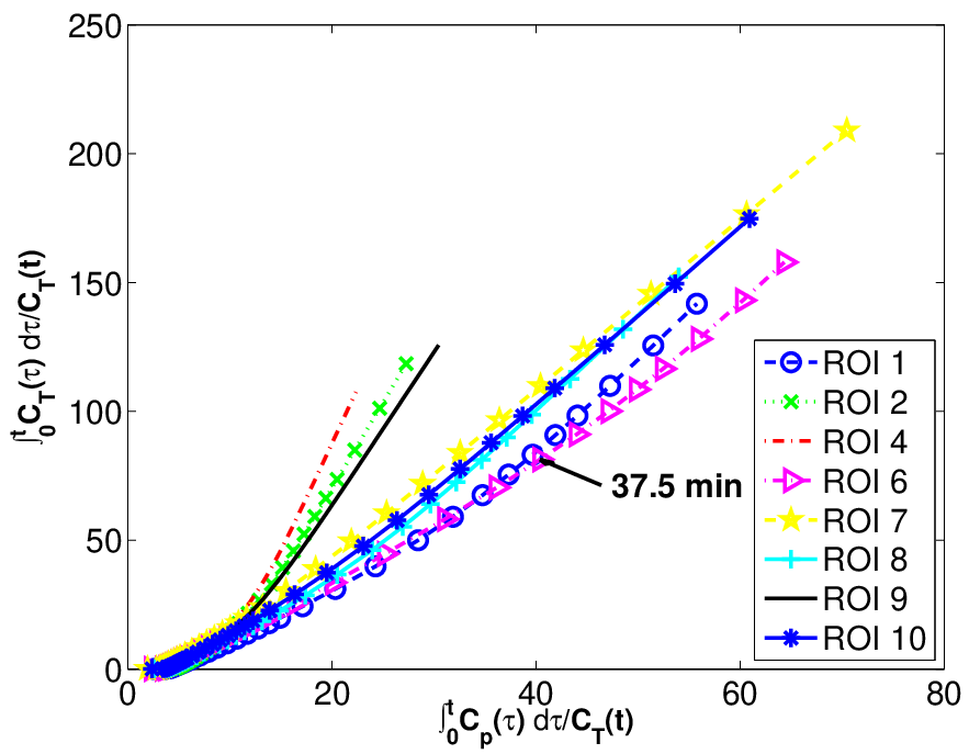
We illustrate the relation between the bias in the estimate of DV calculated by Logan-GA and in Figure 8. As discussed in Section 2.2, a small value of may cause a large variation in . This graph verifies that the magnitude of the bias decreases as increases, further verifying that large bias in DV may arise purely due to modeling assumptions in the absence of noise in the data.

5.2 The effects of quadrature error
Both Logan-GA and MA1, (2) and (3) resp., require the calculation of integrals and . Assume the noise-free measurements are derived from the integral over the th frame duration. Thus we can easily recover its integral without introducing error while quadrature error for calculation of due to using a limited number of plasma samples is unavoidable. The accuracy of the numerical quadrature impacts the accuracy of the parameter estimates. Note that we classify the noise effects as another source of bias in DV.
We recalculate the DV for the experiments reported in Section 4.2, but now using numerical quadrature for calculation of with data sampled one time point per time frame. The bias for each ROI of the estimated DV using minutes scan data with minutes is , , , , , , , , , and when calculated using Logan-GA, and , , , , , , , , , and calculated using MA1. It is interesting to note that the DV calculated for ROI 7 is no longer an over-estimate. This does not contradict the result of Theorem 1, which predicts that the DV for ROI 7 will be over-estimated due to model error, provided that the other aspects of the calculation are accurate. Now using a less accurate quadrature the negative bias due to quadrature error canceled the positive bias due to the model error. Indeed, for all eleven test cases the impact of the less accurate quadrature is to shift the bias down, i.e. it is more negative as compared to the equivalent more accurate calculations shown in Table 2.
5.3 Bias and classification between AD and NC subjects
In the eleven simulated ROIs, large under-estimation of the DV calculated by Logan-GA and MA1 is observed for ROIs 1 (NC Cort), 3 (NC PCG) and 6 (AD Cere). A lower value of the DV in the cortical regions of NCs and in the cerebellum for AD subjects will result in under-estimation of the DVR for NCs and over-estimation of the DVR for AD subjects when the cerebellum is used as the reference region for the DVR calculation. Thus, the difference between AD and NC can be artificially enhanced, and viewed as a positive outcome associated with the bias of Logan-GA and MA1. This conclusion, however, can not be generalized. It is unknown whether it is always the case that AD/NC have small/large in cerebellar regions and relatively large/small in cortical regions. Confirmation of these assertions would suggest, based on the discussion in Sections 2.2 and 5.1, that the DVR is over-estimated for AD subjects and under-estimated for healthy subjects (also see Figure 8). In addition, more subtle differences, such as the ones between mild cognitive impairment (MCI) and NC, or among NC with differential genetic risk for AD, may make the effects of bias much less predictable. Consequently, we evaluate the quantification methods based on their bias because the goal of these methods is to estimate the DV as accurately as possible.
5.4 When does MA1 fail?
As noted in Section 4.5, MA1 generates some results with negative DVs. Such results are reported as unsuccessful in Ichise’s original paper [5]. Careful study of these results shows that the negative DVs arise when has the wrong sign. For most radioligand binding studies is a small positive number because , which is usually larger than , see Remark (1) of Algorithm 1. Thus a small error in the estimate of due to large noise in the data may change its sign. This in turn impacts the sign of the estimate of the DV.
6 Conclusions
In this article, we quantified the model error in estimating distribution volume using graphical analysis methods. We described the conditions under which the DV is either over- or under-estimated, and quantified the bias caused by model error. We validated our findings through simulations with noise-free data. To reduce the impact of model error, we added a simple nonlinear term to the fundamental linear model MA0, and presented a new algorithm for its solution. Simulations with noisy data demonstrate that the new algorithm is cost-effective and robust even for shorter scan durations. For PIB-PET studies, the new method using shorter scan data ( minutes) outperforms, or is at least as good as, Logan-GA, MA1 and KA methods using longer scan data ( minutes). The proposed approach can be easily extended for DVR estimation. This is a focus of our future work.
7 Acknowledgment
This work was supported by grants from the state of Arizona (to Drs. Guo, Reiman, Chen and Renaut), the NIH (R01 AG031581, R01 MH057899 and P30 AG19610 to Dr. Reiman) and the NSF (DMS 0652833 to Dr. Renaut and DMS 0513214 to Drs. Renaut and Guo). The authors thank researchers from the University of Pittsburgh for their published findings, including information about PiB input function and rate constants.
8 Appendix A: fundamental theory for Corollary 1
Here we present the theoretical result from which Theorem 1 is obtained. We use the notation that , , , and , , , , are vectors with entries and , resp. The notation and denotes component wise division and multiplication, namely entries and , is and is the Euclidean norm. We call decreasing (increasing) if (), and non-constant decreasing (non-constant increasing) if it is decreasing (increasing) and at least one of the () signs is strict, (). If all of the () signs are strict, we call strictly decreasing (strictly increasing). A vector is constant if for some constant and for all .
Lemma 1.
In the above Chebyshev’s sum inequalities the numbers are not required to be positive and the equality is true if and only if one of the two vectors, or , is a constant vector. If and are positive vectors, the Chebyshev’s sum inequalities can be expressed as and .
Lemma 2.
If , and are positive real vectors, of which is a increasing vector and is a decreasing vector, then
- 1.
if is a non-constant increasing vector. The inequality is strict if is strictly increasing.
- 2.
if is a non-constant decreasing vector. The inequality is strict if is strictly increasing.
- 3.
if is a constant vector,
- 4.
if is a non-constant decreasing vector. The inequality is strict if is strictly increasing.
- 5.
if is a non-constant increasing vector. The inequality is strict if is strictly increasing.
- 6.
if is a constant vector.
Proof.
We only prove the first case. The proof for the other items follows similarly. We use mathematical induction. For the lowest dimension ,
The last reduction follows from the monotonicity of , , which implies , and the non-constant increasing assumption of , which guarantees . When is strictly increasing . Under this condition for . Assuming the inequality is true for dimension , i.e.
then for
The last reduction is based on the monotonicity of and . When is strictly increasing for all the inequality will be strict because at least one of the terms is positive based on the monotonicity condition. The result thus follows by induction for all integers . ∎
The following corollary now follows immediately by observing that increases when increases and decreases when decreases.
Corollary 2.
If , and are positive real vectors, of which is a strictly increasing vector and is a decreasing vector, then
- 1.
if is a decreasing vector.
- 2.
if is an increasing vector.
Lemma 3.
If , , and are positive real vectors, of which is strictly increasing, is decreasing, and , , and satisfy ; and ; then
- 1.
the estimated solution and exact solution are related by
- (a)
if is a non-constant decreasing vector,
- (b)
if is a non-constant increasing vector,
- (c)
if is a constant vector;
- (a)
- 2.
the following inequality is true without any monotonicity assumptions:
(24) - 3.
the sign of the intercept is determined as follows:
- (a)
if is a non-constant decreasing vector,
- (b)
if is a non-constant increasing vector,
- (c)
if is a constant vector;
- (a)
- 4.
given , the LS solution of for is ;
- 5.
given , the LS solution of for and the true solution have the same relationship as stated in the first conclusion of this theorem.
Proof.
It is easy to verify that the LS solution of is
The proof then follows as outlined below:
- 1.
- 2.
- 3.
- 4.
This result is easily verified.
- 5.
∎
We now transform the exact equation to and rewrite the results using vectors , and . Correspondingly, we find the LS solution of for , .
Corollary 3.
If , and are positive, of which is strictly increasing, , , and satisfy ; and , then
- 1.
the estimated solution and the exact solution are related by
- (a)
if is a non-constant decreasing vector,
- (b)
if is a non-constant increasing vector,
- (c)
if is a constant vector;
Moreover, the following inequality is true without any monotonicity assumptions.
(27) - (a)
- 2.
The sign of the intercept is determined as follows:
- (a)
if is a non-constant decreasing vector,
- (b)
if is a non-constant increasing vector,
- (c)
if is a constant vector.
In addition,
- (a)
if is a non-constant decreasing vector,
- (b)
if is a non-constant increasing vector,
- (c)
if is a constant vector;
- (a)
- 3.
Given , the LS solution of for is ;
- 4.
Given , the LS solution of for and the true solution are related as stated in the first conclusion of this theorem.
9 Appendix B: component-wise perturbation analysis for LS solution of (18)
In Remark 2, we claimed that “the estimate of DV is much more robust to noise in the formulation than are the estimates of and because is much larger than both and for ”. Here we present a theoretical explanation, which is helpful for algorithm design in quantification. Instead of considering a general linear equation, which is out of the range of this paper, we assume a system of equations with only two independent variables . The two columns of the system matrix are denoted by and , i.e. .
Theorem 1.
Suppose the linear system , for , has the exact solution , the uncorrelated noise vector obeys a multi-variable Gaussian distribution with zero means and common variance and that . Then least squares solution has the following statistical properties
- 1.
and , and
- 2.
.
Proof.
We assume matrix has the following singular value decomposition
| (29) |
in which . Then
where
Because is an unitary matrix and we immediately derive the the following inequality from equation (29):
This inequality is equivalent to which implies , i.e. and , and . If we denote the two rows of matrix by and than
Because and we conclude If we let and be the two rows of matrix then and because is unitary. Thus Let
It is clear and because the means of are zero, and and resp.. Therefore . Because we conclude and ∎
This result is illustrated by the following simple example:
The first column is much larger than the second column. If we add noise to the right hand side, i.e. and , and perform simulation with realizations the distribution of the resulted and are illustrated in Figure 9. These results are consistent with the conclusions in Theorem 1.
![[Uncaptioned image]](0904.2634v1/histsolutions.png)
10 Appendix C: derivation for equation (12)
References
- [1] C. S. Patlak, R. G. Blasberg, J. D. Fenstermacher, Graphical evaluation of blood-to-brain transfer constants from multiple-time uptake data, J. Cereb. Blood Flow Metab. 3 (1) (1983) 1–7.
- [2] C. S. Patlak, R. G. Blasberg, Graphical evaluation of blood-to-brain transfer constants from multiple-time uptake data. Generalizations, J. Cereb. Blood Flow Metab. 5 (4) (1985) 584–590.
- [3] J. Logan, J. S. Fowler, N. D. Volkow, A. P. Wolf, S. L. Dewey, D. J. Schlyer, R. R. MacGregor, R. Hitzemann, B. Bendriem, S. J. Gatley, Graphical analysis of reversible radioligand binding from time-activity measurements applied to [N-11C-methyl]-(-)-cocaine PET studies in human subjects, J. Cereb. Blood Flow Metab. 10 (1990) 740–747.
- [4] M. Slifstein, M. Laruelle, Effects of statistical noise on graphic analysis of PET neuroreceptor studies, J. Nucl. Med. 41 (12) (2000) 2083–8.
- [5] M. Ichise, H. Toyama, R. Innis, R. Carson, Strategies to improve neuroreceptor parameter estimation by linear regression analysis., J. Cereb. Blood Flow Metab. 22 (10) (2002) 1271–81.
- [6] J. Logan, A review of graphical methods for tracer studies and strategies to reduce bias, Nuclear Medicine and Biology 30 (8) (2003) 833–844.
- [7] G. Blomqvist, On the construction of functional maps in positron emission tomography, J. Cereb. Blood Flow Metab. (4) (1984) 629–632.
- [8] D. Feng, S. Huang, An unbiased parametric imaging algorithm for nonuniformly sampled biomedical system parameter estimation, IEEE Trans. Med. Imag. 15 (4) (1996) 512–518.
- [9] J. Logan, J. Fowler, N. Volkow, Y. Ding, G. Wang, D. Alexoff, A strategy for removing the bias in the graphical analysis method, J. Cereb. Blood Flow Metab. 21 (3) (2001) 307–20.
- [10] J. Varga, Z. Szabo, Modified regression model for the Logan plot, J. Cereb. Blood Flow Metab. 22 (2) (2002) 240–4.
- [11] G. H. Golub, C. V. Loan, An anlysis of the total least squares problem, SIAM J. Num. Anal. 17 (1980) 883–893.
- [12] R. Ogden, Estimation of kinetic parameters in graphical analysis of PET imaging data, Stat. Med. 22 (22) (2003) 3557–68.
- [13] R. Buchert, F. Wilke, J. van den Hoff, J. Mester, Improved statistical power of the multilinear reference tissue approach to the quantification of neuroreceptor ligand binding by regularization, J. Cereb. Blood Flow Metab. 23 (5) (2003) 612–620.
- [14] A. Joshi, J. A. Fessler, R. A. Koeppe, Improving PET receptor binding estimates from Logan plots using principal component analysis, J. Cereb. Blood Flow Metab. 28 (4) (2008) 852–865.
- [15] Y. Zhou, W. Ye, J. R. Brašić, A. H. Crabb, J. Hilton, D. F. Wong, A consistent and efficient graphical analysis method to improve the quantification of reversible tracer binding in radioligand receptor dynamic PET studies, NeuroImage, 44 (3) (2009) 661–670.
- [16] C. A. Mathis, Y. Wang, D. P. Holt, G. F. Huang, M. L. Debnath, W. E. Klunk, Synthesis and evaluation of 11C-labeled 6-substituted 2-aryl benzothiazoles as amyloid imaging agents, J. Med. Chem. 46 (2003) 2740–2755.
- [17] J. J. Frost, K. H. Douglass, H. S. Mayberg, R. F. Dannals, J. M. Links, A. A. Wilson, H. T. Ravert, W. C. Crozier, H. N. J. Wagner, Multicompartmental analysis of [11C]-carfentanil binding to opiate receptors in humans measured by positron emission tomography, J. Cereb. Blood Flow Metab. 9 (1989) 398–409.
- [18] M. Slifstein, M. Laruelle, Models and methods for derivation of in vivo neuroreceptor parameters with PET and SPECT reversible radiotracers, Nucl. Med. Biol. 28 (2001) 595–608.
- [19] R. N. Gunn, S. R. Gunn, F. E. Turkheimer, J. A. D. Aston, V. J. Cunningham, Positron emission tomography compartmental models, J. Cereb. Blood Flow Metab. 21 (2001) 635–652.
- [20] K. R. Godfrey, Compartmental Models and Their Application, Academic Press, 1983.
- [21] J. C. Price, W. E. Klunk, B. J. Lopresti, X. Lu, J. A. Hoge, S. K. Ziolko, D. P. Holt, C. C. Meltzer, S. T. DeKosky, C. A. Mathis, Kinetic modeling of amyloid binding in humans using PET imaging and Pittsburgh compound-B, J. Cereb. Blood Flow Metab.. 25 (11) (2005) 1528–1547.
- [22] R. N. Gunn, A. A. Lammertsma, S. P. Hume, V. J. Cunningham, Parametric imaging of ligand-receptor binding in PET using a simplified reference region model, NeuroImage 6 (4) (1997) 279–287.
- [23] M. Yaqub, N. Tolboom, R. Boellaard, B. N. M. van Berckel, E. W. van Tilburg, G. Luurtsema, P. Scheltens, A. A. Lammertsma, Simplified parametric methods for [(11)C]PIB studies, Neuroimage 42 (2008) 76–86.
- [24] S. G. Mueller, M. W. Weiner, L. J. Thal, R. C. Petersen, C. R. Jack, W. Jagust, J. Q. Trojanowski, A. W. Toga, L. Beckett, Ways toward an early diagnosis in Alzheimer’s disease: The Alzheimer’s disease neuroimaging initiative (ADNI), Alzheimer’s Dement. 1 (1) (2005) 55–66.
- [25] I. Gradshteyn, I. M. Ryzhik, D. Zwillinger, A. Jeffrey, Table of integrals, series, and products, 6th Edition, Academic Press, 2000.