Stability and Hopf Bifurcation in a
Mathematical Model of
Pluripotent Stem Cell Dynamics

Mostafa Adimy^† Fabien Crauste^† and Shigui Ruan Note: Research was partially supported by the NSERC of Canada and the College of Arts and Sciences at the University of Miami. On leave from Dalhousie University, Halifax, Canada.

Year 2004

Abstract

We study a mathematical model describing the dynamics of a pluripotent stem cell population involved in the blood production process in the bone marrow. This model is a differential equation with a time delay. The delay describes the cell cycle duration and is uniformly distributed on an interval. We obtain stability conditions independent of the delay. We also show that the distributed delay can destabilize the entire system. In particularly, it is shown that Hopf bifurcations can occur.

^†Laboratoire de Mathématiques Appliquées, FRE 2570,

Université de Pau et des Pays de l’Adour,

Avenue de l’université, 64000 Pau, France.

E-mail: mostafa.adimy@univ-pau.fr, fabien.crauste@univ-pau.fr

^∗Department of Mathematics, University of Miami,

P. O. Box 249085, Coral Gables, FL 33124-4250, USA.

E-mail: ruan@math.miami.edu

Keywords: Blood production system, stem cells, delay differential equations, stability, Hopf bifurcation.

1 Introduction

Blood production process, called hematopoiesis, is one of the major biological phenomena occurring in human body. It takes place in the bone marrow where pluripotent stem cells give birth to mature cells. After ejecting their nuclei, these cells enter the bloodstream and become blood cells.

According to the study of Burns and Tannock [4], the population of pluripotent stem cells can be divided into two distinct groups: quiescent cells and proliferating cells. Mathematical models describing the dynamics of this cell population have been studied since the end of the seventies, in particularly by Mackey [9, 10]. We refer to the review articles by Haurie et al. [8] and Mackey et al. [12] for further study and more references on this topic. More recently, Pujo-Menjouet et al. [14] and Pujo-Menjouet and Mackey [15] proved the existence of a Hopf bifurcation for the hematopoiesis model proposed in [9]. In all these works, the authors assumed that the proliferating phase duration is constant. Mathematically, this means that the delay in their models is a discrete delay. However, experimental data (see Bradford et al. [3]) indicate that cells do not spend the same time in the proliferating phase.

In this paper, taking into account this assumption, we assume that the delay (or proliferating phase duration) is uniformly distributed on an interval. The main objective is to investigate the effect of time delay on the dynamical solutions. It is shown that there exist some critical values of time delay such that a local Hopf bifurcation occurs at the non-trivial equilibrium.

The paper is organized as follows. In section 2, we present our model, which is given in equation (1). In section 3, we derive stability conditions for the two equilibria of equation (1) which do not depend on the delay. We show the existence of Hopf bifurcations at the non-trivial equilibrium in section 4. A brief discussion is given in section 5.

2 The Model

Pluripotent stem cells can be either in a resting phase, also known as $G_{0}$ -phase, or in a proliferating phase. In the resting phase, they can die at a constant rate $\delta\geq 0$ , which also includes the cellular differentiation, or be introduced in the proliferating phase at a rate $\beta$ . According to the work of Sachs [16], $\beta$ is assumed to depend on the resting phase population.

In the proliferating phase, which is in fact the so-called cell cycle, pluripotent stem cells are committed to divide and give birth to two daughter cells at the end of this phase. The two daughter cells enter directly the resting phase and complete the cycle. We assume that proliferating cells divide according to a uniform law $f$ on an interval $[\tau_{min},\tau]$ with $0\leq\tau_{min}<\tau<+\infty$ . This assumption comes from the fact that, even if only a little is known about phenomena involved in hematopoiesis, there are strong evidences (see Bradford et al. [3]) indicating that cells do not divide at the same age. The function $f$ is then defined by

f(r)=\left\{\begin{array}[]{ll}\displaystyle\frac{1}{\tau-\tau_{min}},&\qquad\textrm{ if }r\in[\tau_{min},\tau],\\ 0,&\qquad\textrm{ otherwise.}\end{array}\right.

Let $x(t)$ denote the pluripotent stem cell population density (cells/kg) at time $t\geq 0$ . It satisfies the nonlinear delay differential equation

x^{\prime}(t)=-\big(\delta+\beta(x(t))\big)x(t)+\frac{2}{\tau-\tau_{min}}\int_{\tau_{min}}^{\tau}\beta(x(t-r))x(t-r)dr.

(1)

The first term in the right-hand side of equation (1) accounts for the cellular loss due to mortality and cellular differentiation, $\delta x(t)$ , and introduction in the cell cycle, $\beta(x(t))x(t)$ . The second term is for the division of proliferating cells into two daughter cells during mitosis. Proliferating cells are in fact resting cells introduced in the proliferating phase one generation earlier, so that the quantity $\beta(x(t-r))x(t-r)$ appears with a time delay. The factor 2 is, of course, for the division of each proliferating cell into two daughter cells.

In the following, the rate of reintroduction in the proliferating compartment $\beta$ is taken to be a monotone and decreasing Hill function, given by

\beta(x)=\beta_{0}\frac{\theta^{n}}{\theta^{n}+x^{n}}\qquad\textrm{ for }x\geq 0.

The coefficient $\beta_{0}>0$ is the maximum rate of reintroduction, $\theta\geq 0$ is the $G_{0}$ -phase population density for which the rate of re-entry $\beta$ attains its maximum rate of change with respect to the resting phase population, and $n\geq 0$ describes the sensitivity of $\beta$ with changes in the population. This function was firstly used in hematopoiesis models by Mackey [9] in 1978.

In [9] and [11], Mackey gave values of the above parameters for a normal human body production. These values are

\delta=0.05\textrm{ d}^{-1},\quad\beta_{0}=1.77\textrm{ d}^{-1}\quad\textrm{ and }\quad n=3.

(2)

The value of $\theta$ is usually $\theta=1.62\times 10^{8}\textrm{ cells/kg}.$ However, since we shall study the qualitative behavior of the pluripotent stem cells population, the value of $\theta$ is not really important and could be normalized without loss of generality.

Now if we consider an initial continuous nonnegative function $\varphi$ defined on $[-\tau,0]$ , then the equation (1) has a unique continuous and nonnegative solution $x^{\varphi}(t)$ , defined for $t\geq-\tau$ , such that

x^{\varphi}(s)=\varphi(s)\qquad\textrm{ for }s\in[-\tau,0].

This can be obtained by using the results in Hale and Verduyn Lunel [7].

Notice that equation (1) has at most two equilibria, the trivial equilibrium $x\equiv 0$ and a non-trivial positive equilibrium $x\equiv x^{*}$ . The trivial equilibrium always exists and corresponds to the extinction of the population.

Proposition 2.1.

Equation (1) has a non-trivial positive equilibrium $x\equiv x^{*}$ if and only if

\beta_{0}>\delta>0.

(3)

In this case, $x^{*}$ is explicitly given by

x^{*}=\theta\bigg(\frac{\beta_{0}}{\delta}-1\bigg)^{1/n}.

Proof.

Let $x^{*}$ be an equilibrium of equation (1). Then $x^{*}$ satisfies

x^{*}\big(\beta(x^{*})-\delta\big)=0.

Consequently, equation (1) has a non-trivial equilibrium if and only if the equation

\beta(x^{*})=\delta

has a non-trivial solution. Since the function $\beta$ is decreasing and positive with $\beta(0)=\beta_{0}$ , then equation (1) has a non-trivial equilibrium if and only if condition (3) holds. ∎

In the next section, we shall study the stability of the two equilibria of equation (1).

3 Stability

Throughout this section, we are interested in the stability of the equilibria of equation (1), in particularly the stability of the non-trivial equilibrium $x\equiv x^{*}$ . We start by giving a result on the global stability of the trivial equilibrium of (1).

Theorem 3.1.

The trivial equilibrium $x\equiv 0$ of equation (1) is globally stable if

\beta_{0}<\delta.

Proof.

The proof uses a similar technique employed by Adimy and Crauste [1]. It is based on the construction of a Lyapunov functional.

Denote by $C^{+}$ the space of all continuous nonnegative functions on $[-\tau,0]$ . Let $B$ be the function defined by

B(x)=\int_{0}^{x}\beta(s)s\ ds\qquad\textrm{ for }x\geq 0.

Consider the mapping $J:C^{+}\to[0,+\infty)$ defined, for $\varphi\in C^{+}$ , by

J(\varphi)=B(\varphi(0))+\frac{1}{\tau-\tau_{min}}\int_{\tau_{min}}^{\tau}\int_{-r}^{0}\Big(\beta(\varphi(a))\varphi(a)\Big)^{2}dadr.

Then,

\dot{J}(\varphi)=\dot{\varphi}(0)\beta(\varphi(0))\varphi(0)+\frac{1}{\tau-\tau_{min}}\int_{\tau_{min}}^{\tau}\big(\beta(\varphi(0))\varphi(0)\big)^{2}-\big(\beta(\varphi(-r))\varphi(-r)\big)^{2}dr.

Since

\dot{\varphi}(0)=-\big(\delta+\beta(\varphi(0))\big)\varphi(0)+\frac{2}{\tau-\tau_{min}}\int_{\tau_{min}}^{\tau}\beta(\varphi(-r))\varphi(-r)dr,

we obtain that

\begin{array}[]{rcl}\dot{J}(\varphi)&=&-\big(\delta+\beta(\varphi(0))\big)\beta(\varphi(0))\varphi^{2}(0)+\displaystyle\frac{2}{\tau-\tau_{min}}\int_{\tau_{min}}^{\tau}\big(\beta(\varphi(0))\varphi(0)\big)^{2}dr\\ &&-\displaystyle\frac{1}{\tau-\tau_{min}}\int_{\tau_{min}}^{\tau}\big(\beta(\varphi(0))\varphi(0)-\beta(\varphi(-r))\varphi(-r)\big)^{2}dr.\end{array}

Hence,

\dot{J}(\varphi)\leq-\big(\delta-\beta(\varphi(0))\big)\beta(\varphi(0))\varphi(0)^{2}.

Let $\alpha$ be the function defined, for $x\geq 0$ , by

\alpha(x)=(\delta-\beta(x))\beta(x)x^{2}.

Assume that $\beta_{0}<\delta.$ Since $\beta$ is a decreasing function, it follows that the function $x\mapsto\delta-\beta(x)$ is positive for $x\geq 0$ . Hence, $\alpha$ is nonnegative on $[0,+\infty)$ and $\alpha(x)=0$ if and only if $x=0$ . Consequently, the mapping $J$ is a Lyapunov functional when $\beta_{0}<\delta$ . We then deduce that the trivial equilibrium of (1) is globally stable. ∎

The result in Theorem 3.1 describes the fact that when $x\equiv 0$ is the only equilibrium of (1), the population is doomed to extinction except when $\beta_{0}=\delta$ .

Now we focus on the stability of the positive equilibrium $x\equiv x^{*}$ of equation (1). To ensure the existence of the equilibrium $x\equiv x^{*}$ , we assume that condition (3) holds; that is,

\beta_{0}>\delta>0.

We do not expect to obtain conditions for the global stability of $x\equiv x^{*}$ . However, local stability results can be obtained by linearizing equation (1) about $x^{*}$ . Set

\beta^{*}:=\frac{d}{dx}\Big(\beta(x)x\Big)\Big|_{x=x^{*}}=\delta\bigg(1-n\frac{\beta_{0}-\delta}{\beta_{0}}\bigg).

(4)

The linearization of equation (1) at $x^{*}$ is

x^{\prime}(t)=-(\delta+\beta^{*})x(t)+\frac{2\beta^{*}}{\tau-\tau_{min}}\int_{\tau_{min}}^{\tau}x(t-r)dr.

The characteristic equation of (1) is given by

\Delta(\lambda):=\lambda+\delta+\beta^{*}-\frac{2\beta^{*}}{\tau-\tau_{min}}\int_{\tau_{min}}^{\tau}e^{-\lambda r}dr=0.

(5)

We now state and prove our first result on the stability of $x\equiv x^{*}$ .

Theorem 3.2.

Assume that

n\frac{\beta_{0}-\delta}{\beta_{0}}\leq 1.

Then the non-trivial equilibrium $x\equiv x^{*}$ of equation (1) is locally asymptotically stable.

Proof.

We show, in fact, that $x^{*}$ is stable when $\beta^{*}\geq 0$ . By the definition of $\beta^{*}$ given by (4), it follows that

\beta^{*}\geq 0\qquad\textrm{ if and only if }\qquad n\frac{\beta_{0}-\delta}{\beta_{0}}\leq 1.

So we assume that $\beta^{*}\geq 0$ .

We first assume that $\Delta(\lambda)$ , given by (5), is a real function. Then, $\Delta(\lambda)$ is continuously differentiable and its first derivative is given by

\frac{d\Delta}{d\lambda}(\lambda)=1+\frac{2\beta^{*}}{\tau-\tau_{min}}\int_{\tau_{min}}^{\tau}re^{-\lambda r}dr.

(6)

One can see that $d\Delta/d\lambda$ is positive for $\lambda\in\mathbb{R}$ as soon as $\beta^{*}\geq 0$ . Moreover,

\lim_{\lambda\to-\infty}\Delta(\lambda)=-\infty\qquad\textrm{ and }\qquad\lim_{\lambda\to+\infty}\Delta(\lambda)=+\infty.

Consequently, $\Delta(\lambda)$ has a unique real root $\lambda_{0}$ . Since

\Delta(0)=\delta-\beta^{*}=n\delta\Big(1-\frac{\delta}{\beta_{0}}\Big)>0,

we deduce that $\lambda_{0}<0$ .

Now, we show that if $\lambda$ is a characteristic root of equation (5), then $Re(\lambda)\leq\lambda_{0}$ . By contradiction, we assume that there exists a characteristic root $\lambda=\mu+i\omega$ of equation (5) such that $\mu>\lambda_{0}$ . By considering the real part of $\Delta(\lambda)$ , we obtain that

\mu+\delta+\beta^{*}-\frac{2\beta^{*}}{\tau-\tau_{min}}\int_{\tau_{min}}^{\tau}e^{-\mu r}\cos(\omega r)dr=0.

Consequently,

\mu-\lambda_{0}=\frac{2\beta^{*}}{\tau-\tau_{min}}\int_{\tau_{min}}^{\tau}\big(e^{-\mu r}\cos(\omega r)-e^{-\lambda_{0}r}\big)dr<0.

This yields a contradiction. We conclude that every characteristic root $\lambda$ of (5) is such that $Re(\lambda)\leq\lambda_{0}$ . Hence, all characteristic roots of (5) have negative real parts and the equilibrium $x\equiv x^{*}$ is locally asymptotically stable. ∎

When $\beta^{*}<0$ , that is, when

1<n\frac{\beta_{0}-\delta}{\beta_{0}},

the stability cannot occur for all values of $\tau_{min}$ and $\tau$ . In particularly, we shall show that a Hopf bifurcation can occur (see Theorem 4.1). However, we can still have the stability of the non-trivial equilibrium $x\equiv x^{*}$ for values of $n$ , $\beta_{0}$ and $\delta$ if $n(\beta_{0}-\delta)/\beta_{0}$ is not too large. This will be considered in the next theorem.

To present the results, without loss of generality we assume that

\tau_{min}=0.

We want to point out that the results we are going to show remain true when $\tau_{min}>0$ , but the proof is more complicated.

Define a function $K$ , for $x\geq 0$ , by

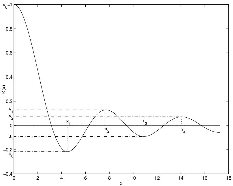
K(x)=\frac{\sin(x)}{x}

(7)

and let $x_{1}$ be the unique solution of the equation

x_{1}=\tan(x_{1}),\qquad x_{1}\in(\pi,\frac{3\pi}{2}).

Set

u_{0}:=\cos(x_{1})\in(-1,0).

Then $K^{\prime}(x_{1})=0$ and

u_{0}=K(x_{1})=\min_{x\geq 0}K(x).

(8)

We have the following local stability theorem.

Theorem 3.3.

Assume that

1<n\frac{\beta_{0}-\delta}{\beta_{0}}<\frac{2(1-u_{0})}{1-2u_{0}}.

(9)

Then the non-trivial equilibrium $x\equiv x^{*}$ of equation (1) is locally asymptotically stable.

Proof.

Let us assume that (9) holds. Then $\beta^{*}<0$ , $\delta+\beta^{*}>0$ and

\frac{\delta+\beta^{*}}{2\beta^{*}}<u_{0}.

(10)

By contradiction, assume that there exists a characteristic root $\lambda=\mu+i\omega$ of (5) with $\mu>0$ . Then,

\mu=-(\delta+\beta^{*})+\frac{2\beta^{*}}{\omega\tau}\int_{0}^{\omega\tau}e^{-\displaystyle\frac{\mu}{\omega}r}\cos(r)dr

and

\omega=-\frac{2\beta^{*}}{\omega\tau}\int_{0}^{\omega\tau}e^{-\displaystyle\frac{\mu}{\omega}r}\sin(r)dr.

Integrating by parts, we obtain that

2\mu=-(\delta+\beta^{*})+2\beta^{*}e^{-\mu\tau}K(\omega\tau).

Consequently,

\mu<-(\delta+\beta^{*})+2\beta^{*}e^{-\mu\tau}K(\omega\tau).

If $\omega\tau$ is such that

\sin(\omega\tau)\geq 0,

then

2\beta^{*}K(\omega\tau)<0

and

\mu<-(\delta+\beta^{*})\leq 0.

So we obtain a contradiction.

Similarly, if $\omega\tau$ is such that

\sin(\omega\tau)<0,

then, from (8) and (10), we deduce that

\frac{\delta+\beta^{*}}{2\beta^{*}}\leq K(\omega\tau).

It implies that

\delta+\beta^{*}\geq 2\beta^{*}K(\omega\tau)>2\beta^{*}e^{-\mu\tau}K(\omega\tau).

Therefore,

\mu<-(\delta+\beta^{*})+2\beta^{*}K(\omega\tau)\leq 0.

Again we obtain a contradiction. Hence, all characteristic roots $\lambda$ of (5) are such that $Re(\lambda)\leq 0$ .

Now, we assume that (5) has a purely imaginary characteristic root $\lambda=i\omega$ . Then $\omega$ and $\tau$ satisfy

K(\omega\tau)=\frac{\delta+\beta^{*}}{2\beta^{*}}.

(11)

Using (8) and (10), we obtain a contradiction. Consequently, (11) has no solution and equation (5) does not have purely imaginary roots. We conclude that all characteristic roots of (5) have negative real parts and $x\equiv x^{*}$ is locally asymptotically stable. ∎

From Theorems 3.2 and 3.3, it follows that the non-trivial equilibrium $x\equiv x^{*}$ of equation (1) is locally asymptotically stable when

0\leq n\frac{\beta_{0}-\delta}{\beta_{0}}<\frac{2(1-u_{0})}{1-2u_{0}}.

(12)

We are going to show that as soon as condition (12) does not hold, then the equilibrium can be destabilized. In the next section, we shall show that if condition (10) does not hold, then a Hopf bifurcation indeed occurs at $x\equiv x^{*}$ .

4 Hopf Bifurcations

In this section we are going to show that the non-trivial equilibrium $x\equiv x^{*}$ of equation (1) can be destabilized via Hopf bifurcations. The time delay $\tau$ will be used as a bifurcation parameter. This result is obtained in Theorem 4.1.

Recall that the non-trivial equilibrium $x\equiv x^{*}$ of equation (1) exists if and only if $\beta_{0}>\delta>0.$ In the following, without loss of generality we assume that

\tau_{min}=0.

Again the results still hold when $\tau_{min}>0$ , but the proof is easier to understand when $\tau_{min}=0$ .

We look for purely imaginary roots of $\Delta(\lambda)$ . Of course, we assume that $\beta^{*}<0$ , otherwise $x\equiv x^{*}$ is locally asymptotically stable. Let $\lambda=i\omega$ , with $\omega\in\mathbb{R}$ , be a purely imaginary characteristic root of equation (5). Then, $\tau$ and $\omega$ satisfy the following system

\left\{\begin{array}[]{rcl}\delta+\beta^{*}\big(1-2C(\tau,\omega)\big)&=&0,\\ \omega+2\beta^{*}S(\tau,\omega)&=&0,\end{array}\right.

(13)

where

C(\tau,\omega)=\frac{1}{\tau}\int_{0}^{\tau}\cos(\omega r)dr,\qquad S(\tau,\omega)=\frac{1}{\tau}\int_{0}^{\tau}\sin(\omega r)dr.

First, one can see that $\omega=0$ cannot be a solution of (13). Otherwise

\delta=\beta^{*}<0.

Moreover, if $\omega$ is a solution of system (13), then $-\omega$ is also a solution of (13). Hence, we only look for positive solutions $\omega$ .

One can check that $C(\tau,\omega)$ and $S(\tau,\omega)$ are given, for $\tau>0$ and $\omega>0$ , by

C(\tau,\omega)=\frac{\sin(\omega\tau)}{\omega\tau}=K(\omega\tau),\qquad S(\tau,\omega)=\frac{1-\cos(\omega\tau)}{\omega\tau},

where the function $K$ is defined by (7). Consequently, system (13) can be rewritten as

	$\displaystyle K(\omega\tau)$	$\displaystyle=$	$\displaystyle\frac{\delta+\beta^{}}{2\beta^{}},\vskip 4.30554pt$		(14)
	$\displaystyle\displaystyle\frac{\cos(\omega\tau)-1}{(\omega\tau)^{2}}$	$\displaystyle=$	$\displaystyle\frac{1}{2\beta^{*}\tau}.$		(15)

Consider the sequence

\{x_{k}\}_{k\in\mathbb{N}}:=\{x\geq 0\ ;\ x=\tan(x)\},

(16)

with

0=x_{0}<x_{1}<\cdots<x_{k}<\cdots.

In fact, one can check that

\{x_{k}\}_{k\in\mathbb{N}}=\{x\geq 0\ ;\ K^{\prime}(x)=0\}.

Moreover, for all $k\in\mathbb{N}^{*}$ ,

x_{k}\in(k\pi,k\pi+\frac{\pi}{2}).

Define two sequences $\{u_{k}\}$ and $\{v_{k}\}$ , for $k\in\mathbb{N}$ , by

u_{k}:=\cos(x_{2k+1})<0,\qquad v_{k}:=\cos(x_{2k})>0.

Using the definition of $x_{k}$ , one can see that

u_{k}=K(x_{2k+1})\qquad\textrm{ and }\qquad v_{k}=K(x_{2k}).

Thus, the sequence $\{u_{k}\}_{k\in\mathbb{N}}$ is increasing with $-1<u_{k}<0$ and the sequence $\{v_{k}\}_{k\in\mathbb{N}}$ is decreasing with $v_{0}=1$ and $0<v_{k}<1/2$ for $k\geq 1$ (see Figure 1).

Refer to caption — Figure 1: The graphe of $K(x)$ .

Moreover,

\lim_{k\to+\infty}u_{k}=\lim_{k\to+\infty}v_{k}=0.

Furthermore, one can check that, as soon as $\beta^{*}<0$ ,

\frac{\delta+\beta^{*}}{2\beta^{*}}<1=v_{0}.

Finally, define a function $h$ , for $x\in[-1,1/2)$ , by

h(x)=\frac{2(1-x)}{1-2x}

and set

h(v_{0})=+\infty.

We have the following results about the properties of the function $h.$

Lemma 4.1.

Suppose that

h(u_{0})\leq n\frac{\beta_{0}-\delta}{\beta_{0}}\qquad\textrm{ and }\qquad\delta+\beta^{*}\neq 0.

(i) If $\delta+\beta^{*}>0$ , then there exists $k\in\mathbb{N}$ such that

h(u_{k})\leq n\frac{\beta_{0}-\delta}{\beta_{0}}<h(u_{k+1}).

(ii) If $\delta+\beta^{*}<0$ , then there exists $k\in\mathbb{N}$ such that

h(v_{k+1})\leq n\frac{\beta_{0}-\delta}{\beta_{0}}<h(v_{k}).

Proof.

Since the function $h$ is increasing on the interval $[-1,1/2)$ , we can see that

h(u_{k})\leq n\frac{\beta_{0}-\delta}{\beta_{0}}<h(u_{k+1})

is equivalent to

u_{k}\leq\frac{\delta+\beta^{*}}{2\beta^{*}}<u_{k+1}

and

h(v_{k+1})\leq n\frac{\beta_{0}-\delta}{\beta_{0}}<h(v_{k})

is equivalent to

v_{k+1}\leq\frac{\delta+\beta^{*}}{2\beta^{*}}<v_{k}.

The lemma now follows. ∎

Proposition 4.1.

(i) If

h(u_{k})<n\frac{\beta_{0}-\delta}{\beta_{0}}<h(u_{k+1}),\qquad k\in\mathbb{N},

then system (14)-(15) has exactly $2(k+1)$ solutions $(\tau_{1,1},\omega_{1,1})$ , …, $(\tau_{k+1,1},\omega_{k+1,1})$ and $(\tau_{1,2},\omega_{1,2})$ , …, $(\tau_{k+1,2},\omega_{k+1,2})$ with

\left\{\begin{array}[]{ll}\omega_{l,1}\tau_{l,1}\in((2l-1)\pi,x_{2l-1}),&\quad\textrm{ for }l=1,\dots,k+1,\\ \omega_{l,2}\tau_{l,2}\in(x_{2l-1},2l\pi),&\quad\textrm{ for }l=1,\dots,k+1\end{array}\right.

and

0<\tau_{1,1}<\cdots<\tau_{k+1,1}<\tau_{k+1,2}<\cdots<\tau_{1,2}.

(ii) If

n\frac{\beta_{0}-\delta}{\beta_{0}}=h(u_{k}),\qquad k\in\mathbb{N},

then system (14)-(15) has exactly $2k+1$ solutions $(\tau_{1,1},\omega_{1,1})$ , …, $(\tau_{k+1,1},\omega_{k+1,1})$ and $(\tau_{1,2},\omega_{1,2})$ , …, $(\tau_{k,2},\omega_{k,2})$ with

\left\{\begin{array}[]{ll}\omega_{l,1}\tau_{l,1}\in((2l-1)\pi,x_{2l-1}),&\quad\textrm{ for }l=1,\dots,k,\\ \omega_{l,2}\tau_{l,2}\in(x_{2l-1},2l\pi),&\quad\textrm{ for }l=1,\dots,k,\\ \omega_{k+1,1}\tau_{k+1,1}=x_{2k+1}&\end{array}\right.

and

0<\tau_{1,1}<\cdots<\tau_{k+1,1}<\tau_{k,2}<\cdots<\tau_{1,2}.

(iii) If

h(v_{k+1})<n\frac{\beta_{0}-\delta}{\beta_{0}}<h(v_{k}),\qquad k\in\mathbb{N}^{*},

then system (14)-(15) has exactly $2k+1$ solutions $(\tau_{1,1},\omega_{1,1})$ , …, $(\tau_{k+1,1},\omega_{k+1,1})$ and $(\tau_{1,2},\omega_{1,2})$ , …, $(\tau_{k,2},\omega_{k,2})$ with

\left\{\begin{array}[]{ll}\omega_{1,1}\tau_{1,1}\in(\pi/2,\pi),&\\ \omega_{l,1}\tau_{l,1}\in(x_{l+1},(l+2)\pi),&\qquad\textrm{for }l=2,\dots,k+1,\\ \omega_{l,2}\tau_{l,2}\in((l+1)\pi,x_{l+1}),&\qquad\textrm{for }l=1,\dots,k\end{array}\right.

and

0<\tau_{1,1}<\cdots<\tau_{k+1,1}<\tau_{k,2}<\cdots<\tau_{1,2}.

(iv) If

n\frac{\beta_{0}-\delta}{\beta_{0}}=h(v_{k}),\qquad k\in\mathbb{N}^{*},

then system (14)-(15) has exactly $2k$ solutions $(\tau_{1,1},\omega_{1,1})$ , …, $(\tau_{k,1},\omega_{k,1})$ and $(\tau_{1,2},\omega_{1,2})$ , …, $(\tau_{k,2},\omega_{k,2})$ , with

\left\{\begin{array}[]{ll}\omega_{1,1}\tau_{1,1}\in(\pi/2,\pi),&\\ \omega_{l,1}\tau_{l,1}\in(x_{l},(l+1)\pi),&\quad\textrm{for }l=2,\dots,k,\\ \omega_{l,2}\tau_{l,2}\in((l+1)\pi,x_{l+1}),&\quad\textrm{for }l=1,\dots,k-1,\\ \omega_{k,2}\tau_{k,2}=x_{2k}&\end{array}\right.

and

0<\tau_{1,1}<\cdots<\tau_{k,1}<\tau_{k,2}<\cdots<\tau_{1,2}.

(v) If

h(v_{1})<n\frac{\beta_{0}-\delta}{\beta_{0}}<h(v_{0}),

then system (14)-(15) has a unique solution $(\tau_{1},\omega_{1})$ such that $\tau_{1}>0$ and

\omega_{1}\tau_{1}\in(0,\pi).

Proof.

We only prove $(i)$ when $k=0$ . The other cases can be deduced similarly. Assume that

h(u_{0})<n\frac{\beta_{0}-\delta}{\beta_{0}}<h(u_{1}).

This is equivalent to

u_{0}<\frac{\delta+\beta^{*}}{2\beta^{*}}<u_{1}.

The function $K$ is strictly negative and decreasing on $(\pi,x_{1})$ with $K(y)\in(u_{0},0)$ (see Figure 1). So the equation

K(y)=\frac{\delta+\beta^{*}}{2\beta^{*}}

has a unique solution $y_{1}$ on the interval $(\pi,x_{1})$ . Set

\tau_{1,1}=\frac{(y_{1})^{2}}{2\beta^{*}(\cos(y_{1})-1)}

and $\omega_{1,1}=y_{1}/\tau_{1,1}$ . Then, $(\tau_{1,1},\omega_{1,1})$ is a unique solution of system (14)-(15) satisfying $\omega_{1,1}\tau_{1,1}\in(\pi,x_{1})$ .

Moreover, the function $K$ is strictly negative and increasing on $(x_{1},2\pi)$ with $K(y)\in(u_{0},0)$ , so the equation $K(y)=(\delta+\beta^{*})/2\beta^{*}$ has a unique solution $y_{2}$ on the interval $(x_{1},2\pi)$ . Set

\tau_{1,2}=\frac{(y_{2})^{2}}{2\beta^{*}(\cos(y_{2})-1)}

and $\omega_{1,2}=y_{2}/\tau_{1,2}$ . Then, $(\tau_{1,2},\omega_{1,2})$ is a unique solution of system (14)-(15) which satisfies $\omega_{1,2}\tau_{1,2}\in(x_{1},2\pi)$ .

Furthermore, the function $K$ is nonnegative on $[0,\pi]$ and

u_{1}=K(x_{3})=\min_{x\geq 2\pi}K(x).

Therefore, system (14)-(15) has two solutions, $(\tau_{1,1},\omega_{1,1})$ and $(\tau_{1,2},\omega_{1,2})$ .

Finally, using the fact that

\cos(y_{1})\leq\cos(y_{2}),

we obtain that

\tau_{1,1}<\tau_{1,2}.

This completes the proof. ∎

Lemma 4.1 and Proposition 4.1 give conditions for the existence of pairs of purely imaginary roots of equation (5). In the next proposition, we study the properties of the purely imaginary roots of (5).

Proposition 4.2.

Assume that there exists a $\tau_{c}>0$ such that equation (5) has a pair of purely imaginary roots $\pm i\omega_{c}$ for $\tau=\tau_{c}$ with $\omega_{c}>0$ . If

\omega_{c}\tau_{c}\neq x_{k}\qquad\textrm{ for all }k\in\mathbb{N},

where the sequence $\{x_{k}\}_{k\in\mathbb{N}}$ is defined by (16), then $\pm i\omega_{c}$ are simple roots such that

\left\{\begin{array}[]{ll}\displaystyle\frac{dRe(\lambda)}{d\tau}\Big|_{\tau=\tau_{c}}>0,&\qquad\textrm{ if }\;\;\omega_{c}\tau_{c}\in(x_{2k},x_{2k+1}),\\ \displaystyle\frac{dRe(\lambda)}{d\tau}\Big|_{\tau=\tau_{c}}<0,&\qquad\textrm{ if }\;\;\omega_{c}\tau_{c}\in(x_{2k+1},x_{2k+2}),\quad k\in\mathbb{N}.\end{array}\right.

Proof.

Assume that there exists a $\tau_{c}>0$ such that equation (5) has a pair of purely imaginary roots $\pm i\omega_{c}$ for $\tau=\tau_{c}$ with $\omega_{c}>0$ . Then, $\omega_{c}\tau_{c}$ satisfies system (14)-(15).

Assume that

\omega_{c}\tau_{c}\neq x_{k}\quad\textrm{ for all }k\in\mathbb{N}.

Let us show that $\pm i\omega_{c}$ are simple characteristic roots of (5). Using (6), one can see that $\pm i\omega_{c}$ are simple roots of (5) if

1+2\beta^{*}\displaystyle\frac{\partial S}{\partial\omega}(\tau_{c},\omega_{c})\neq 0\qquad\textrm{ or }\qquad\displaystyle\frac{\partial C}{\partial\omega}(\tau_{c},\omega_{c})\neq 0.

We will show that

\frac{\partial C}{\partial\omega}(\tau_{c},\omega_{c})\neq 0.

A simple computation shows that

\frac{\partial C}{\partial\omega}(\tau_{c},\omega_{c})=\frac{g(\omega_{c}\tau_{c})}{\omega_{c}^{2}\tau_{c}},

where the function $g$ is defined by

g(x)=x\cos(x)-\sin(x)\qquad\textrm{for }x\geq 0.

One can check that $g(x)=0$ if and only if there exists a $k_{0}\in\mathbb{N}$ such that $x=x_{k_{0}}$ . Moreover,

g(x)>0\qquad\textrm{ if and only if }\qquad x\in(x_{2k+1},x_{2k+2}),\ k\in\mathbb{N}.

This yields that

\frac{\partial C}{\partial\omega}(\tau_{c},\omega_{c})<0\quad\textrm{ if }\quad\omega_{c}\tau_{c}\in(x_{2k},x_{2k+1})

and

\frac{\partial C}{\partial\omega}(\tau_{c},\omega_{c})>0\quad\textrm{ if }\quad\omega_{c}\tau_{c}\in(x_{2k+1},x_{2k+2}).

Hence, $\pm i\omega_{c}$ are simple characteristic roots of (5).

Let $\lambda(\tau)=\mu(\tau)+i\omega(\tau)$ be a characteristic root of (5) such that $\lambda(\tau_{c})=\pm i\omega_{c}$ . By separating the real and imaginary parts, we obtain that

\left\{\begin{array}[]{rcl}\mu(\tau)+\delta+\beta^{*}-\displaystyle\frac{2\beta^{*}}{\tau}\int_{0}^{\tau}e^{-\mu(\tau)r}\cos(\omega(\tau)r)dr&=&0,\\ \omega(\tau)+\displaystyle\frac{2\beta^{*}}{\tau}\int_{0}^{\tau}e^{-\mu(\tau)r}\sin(\omega(\tau)r)dr&=&0.\end{array}\right.

We denote by $\mu^{\prime}(\tau)$ (respectively $\omega^{\prime}(\tau)$ ) the first derivative of $\mu(\tau)$ (respectively $\omega(\tau)$ ) with respect to $\tau$ . For $\tau=\tau_{c}$ , we obtain that

\begin{array}[]{l}\mu^{\prime}(\tau_{c})\Big[1+2\beta^{*}\displaystyle\frac{\partial S}{\partial\omega}(\tau_{c},\omega_{c})\Big]\\ \qquad=2\beta^{*}\displaystyle\frac{\partial C}{\partial\omega}(\tau_{c},\omega_{c})\omega^{\prime}(\tau_{c})\vskip 4.30554pt+\displaystyle\frac{2\beta^{*}}{\tau_{c}}\big(\cos(\omega_{c}\tau_{c})-C(\tau_{c},\omega_{c})\big)\end{array}

(17)

and

\begin{array}[]{l}\omega^{\prime}(\tau_{c})\Big[1+2\beta^{*}\displaystyle\frac{\partial S}{\partial\omega}(\tau_{c},\omega_{c})\Big]\\ \qquad=-2\beta^{*}\displaystyle\frac{\partial C}{\partial\omega}(\tau_{c},\omega_{c})\mu^{\prime}(\tau_{c})\vskip 4.30554pt+\displaystyle\frac{2\beta^{*}}{\tau_{c}}\big(S(\tau_{c},\omega_{c})-\sin(\omega_{c}\tau_{c})\big).\end{array}

(18)

We consider two cases. First, assume that

1+2\beta^{*}\displaystyle\frac{\partial S}{\partial\omega}(\tau_{c},\omega_{c})=0.

(19)

One can verify that

1+2\beta^{*}\displaystyle\frac{\partial S}{\partial\omega}(\tau_{c},\omega_{c})=2+(\delta+\beta^{*})\tau_{c}.

Consequently, (19) is equivalent to

\tau_{c}=-\frac{2}{\delta+\beta^{*}}.

(20)

Then, it follows from equation (18) that

\frac{\partial C}{\partial\omega}(\tau_{c},\omega_{c})\mu^{\prime}(\tau_{c})=\frac{S(\tau_{c},\omega_{c})-\sin(\omega_{c}\tau_{c})}{\tau_{c}}.

Moreover, by using (14) and (15), we have

\begin{array}[]{rcl}\displaystyle\frac{S(\tau_{c},\omega_{c})-\sin(\omega_{c}\tau_{c})}{\tau_{c}}&=&\displaystyle\frac{1-\big(\cos(\omega_{c}\tau_{c})+\omega_{c}\tau_{c}\sin(\omega_{c}\tau_{c})\big)}{\omega_{c}\tau_{c}^{2}}\\ &=&-\displaystyle\frac{\delta+\beta^{*}}{4\beta^{*}}\omega_{c}.\end{array}

Hence, (20) implies that

\frac{\partial C}{\partial\omega}(\tau_{c},\omega_{c})\mu^{\prime}(\tau_{c})=\frac{\omega_{c}}{2\beta^{*}\tau_{c}}<0.

Since $\frac{\partial C}{\partial\omega}(\tau_{c},\omega_{c})\neq 0,$ we have

\mu^{\prime}(\tau_{c})\neq 0.

Furthermore, the sign of $\mu^{\prime}(\tau_{c})$ is the same as the sign of $-\frac{\partial C}{\partial\omega}(\tau_{c},\omega_{c}).$

We now assume that

1+2\beta^{*}\displaystyle\frac{\partial S}{\partial\omega}(\tau_{c},\omega_{c})\neq 0.

Then, by using (17) and (18), we obtain that $\mu^{\prime}(\tau_{c})$ satisfies

\begin{array}[]{l}\mu^{\prime}(\tau_{c})\Big[\Big(1+2\beta^{*}\displaystyle\frac{\partial S}{\partial\omega}(\tau_{c},\omega_{c})\Big)^{2}+\Big(2\beta^{*}\displaystyle\frac{\partial C}{\partial\omega}(\tau_{c},\omega_{c})\Big)^{2}\Big]\\ \quad=\displaystyle\frac{2\beta^{*}}{\tau_{c}}\Big[2\beta^{*}\displaystyle\frac{\partial C}{\partial\omega}(\tau_{c},\omega_{c})\big(S(\tau_{c},\omega_{c})-\sin(\omega_{c}\tau_{c})\big)\\ \qquad\qquad+\Big(1+2\beta^{*}\displaystyle\frac{\partial S}{\partial\omega}(\tau_{c},\omega_{c})\Big)\big(\cos(\omega_{c}\tau_{c})-C(\tau_{c},\omega_{c})\big)\Big].\end{array}

Using the definitions of $C$ and $S$ , one can check that

\frac{\partial C}{\partial\omega}(\tau_{c},\omega_{c})\big(S(\tau_{c},\omega_{c})-\sin(\omega_{c}\tau_{c})\big)+\frac{\partial S}{\partial\omega}(\tau_{c},\omega_{c})\big(\cos(\omega_{c}\tau_{c})-C(\tau_{c},\omega_{c})\big)=0.

Hence,

\mu^{\prime}(\tau_{c})\Big[\Big(1+2\beta^{*}\displaystyle\frac{\partial S}{\partial\omega}(\tau_{c},\omega_{c})\Big)^{2}+\Big(2\beta^{*}\displaystyle\frac{\partial C}{\partial\omega}(\tau_{c},\omega_{c})\Big)^{2}\Big]=\displaystyle\frac{2\beta^{*}}{\tau_{c}}\big(\cos(\omega_{c}\tau_{c})-C(\tau_{c},\omega_{c})\big).

Notice that

\frac{\cos(\omega_{c}\tau_{c})-C(\tau_{c},\omega_{c})}{\tau_{c}}=\frac{g(\omega_{c}\tau_{c})}{\omega_{c}\tau_{c}^{2}}=\frac{\omega_{c}}{\tau_{c}}\frac{\partial C}{\partial\omega}(\tau_{c},\omega_{c})\neq 0.

Since $1+2\beta^{*}\displaystyle\frac{\partial S}{\partial\omega}(\tau_{c},\omega_{c})\neq 0$ , it follows that

\Big(1+2\beta^{*}\displaystyle\frac{\partial S}{\partial\omega}(\tau_{c},\omega_{c})\Big)^{2}+\Big(2\beta^{*}\displaystyle\frac{\partial C}{\partial\omega}(\tau_{c},\omega_{c})\Big)^{2}>0.

Consequently, $\mu^{\prime}(\tau_{c})\neq 0$ , and the sign of $\mu^{\prime}(\tau_{c})$ is the same as the sign of $-\frac{\partial C}{\partial\omega}(\tau_{c},\omega_{c}).$

In summary, we have obtained that, for $\tau=\tau_{c}$ , equation (5) has a pair of simple purely imaginary roots $\pm i\omega_{c}$ such that

\left\{\begin{array}[]{ll}\displaystyle\frac{dRe(\lambda)}{d\tau}\Big|_{\tau=\tau_{c}}>0,&\qquad\textrm{ if }\omega_{c}\tau_{c}\in(x_{2k},x_{2k+1}),\\ \displaystyle\frac{dRe(\lambda)}{d\tau}\Big|_{\tau=\tau_{c}}<0,&\qquad\textrm{ if }\omega_{c}\tau_{c}\in(x_{2k+1},x_{2k+2}).\end{array}\right.

This completes the proof. ∎

Remark 1.

If there exists a $k\in\mathbb{N}^{*}$ such that

\omega_{c}\tau_{c}=x_{k},

then either $\pm i\omega_{c}$ are not simple roots of (5) or

\frac{dRe(\lambda)}{d\tau}\Big|_{\tau=\tau_{c}}=0.

Using a similar argument as in the proof of Proposition 4.1, we obtain that

\frac{\partial C}{\partial\omega}(\tau_{c},\omega_{c})=0.

Thus, if

\tau_{c}=-\frac{2}{\delta+\beta^{*}},

then $\pm i\omega_{c}$ are not simple roots of (5). If

\tau_{c}\neq-\frac{2}{\delta+\beta^{*}},

then

\frac{dRe(\lambda)}{d\tau}\Big|_{\tau=\tau_{c}}=0.

In the next theorem, we show that there exists a Hopf bifurcation at the non-trivial equilibrium $x\equiv x^{*}$ of equation (1).

Theorem 4.1.

Assume that

h(u_{0})\leq n\frac{\beta_{0}-\delta}{\beta_{0}}\qquad\textrm{ and }\qquad\delta+\beta^{*}\neq 0.

Then a Hopf bifurcation occurs at $x\equiv x^{*}$ for $\tau=\tau_{0}:=\min_{\omega_{c}\tau_{c}\neq x_{k},\ k\in\mathbb{N}}\tau_{c}$ , where $(\tau_{c},\omega_{c})$ are solutions of (14)-(15), defined in Proposition 4.1. When $0\leq\tau<\tau_{0}$ , the equilibrium $x\equiv x^{*}$ is locally asymptotically stable and it is unstable while $\tau_{0}\leq\tau\leq\tau_{l}$ , where $\tau_{l}$ is the larger value of $\tau_{c}$ such that $\omega_{c}\tau_{c}\in(x_{2k},x_{2k+1})$ , $k\in\mathbb{N}$ .

Proof.

We first check that $x\equiv x^{*}$ is locally asymptotically stable when $\tau\in[0,\tau_{0})$ . Notice that when $\tau\in[0,\tau_{0})$ , equation (5) does not have purely imaginary roots. Let $\tau^{*}>0$ be small enough and fixed. Assume that, for $\tau\in(0,\tau^{*})$ , equation (5) has a characteristic root $\lambda(\tau)=\mu(\tau)+i\omega(\tau)$ with $\mu(\tau)>0$ . Separating the real and imaginary parts, we obtain

\mu(\tau)=-(\delta+\beta^{*})+\frac{2\beta^{*}}{\tau}\int_{0}^{\tau}e^{-\mu(\tau)r}\cos(\omega(\tau)r)dr

and

\omega(\tau)=-\frac{2\beta^{*}}{\tau}\int_{0}^{\tau}e^{-\mu(\tau)r}\sin(\omega(\tau)r)dr.

We deduce that, for $\tau\in(0,\tau^{*})$ ,

|\mu(\tau)|\leq|\delta+\beta^{*}|-2\beta^{*}\qquad\textrm{ and }\qquad|\omega(\tau)|\leq-2\beta^{*}.

Consequently,

\lim_{\tau\to 0}\tau\mu(\tau)=0\qquad\textrm{ and }\qquad\lim_{\tau\to 0}\tau\omega(\tau)=0.

Integrating by parts, we obtain

2\mu(\tau)=-(\delta+\beta^{*})+2\beta^{*}e^{-\tau\mu(\tau)}K(\tau\omega(\tau)).

Since $\mu(\tau)>0$ , we have for $\tau\in(0,\tau^{*})$ that

-(\delta+\beta^{*})+2\beta^{*}e^{-\tau\mu(\tau)}K(\tau\omega(\tau))>0.

When $\tau$ tends to zero, we obtain

\beta^{*}-\delta\geq 0.

However, $\beta^{*}-\delta<0$ . This is a contradiction. Therefore, for $\tau\in(0,\tau^{*})$ , $\mu(\tau)<0$ . Applying Rouché’s Theorem [References, p.248], we obtain that all characteristic roots of (5) have negative real parts when $\tau\in[0,\min(\tau_{c}))$ . Therefore, $x\equiv x^{*}$ is locally asymptotically stable.

Using Lemma 4.1, Propositions 4.1 and 4.2, we conclude to the existence of $\tau_{l}$ . This concludes the proof. ∎

We illustrate the results of Theorem 4.1 in the next corollary.

Corollary 4.1.

Assume that the parameters $\delta$ , $\beta_{0}$ and $n$ are given by (2). Then there exists a unique value $\tau_{c}>0$ such that a Hopf bifurcation occurs at $x\equiv x^{*}$ when $\tau=\tau_{c}$ . When $\tau<\tau_{c}$ , the equilibrium is locally asymptotically stable and becomes unstable when $\tau\geq\tau_{c}$ . Moreover, when $\tau=\tau_{c}$ , equation (1) has a periodic solution with a period close to $46$ days (see Figure 2). The value of $\tau_{c}$ is approximately given by

\tau_{c}\simeq 18\textrm{ days}.

Proof.

With the values given by (2), we obtain

n\frac{\beta_{0}-\delta}{\beta_{0}}\simeq 2.9153>h(v_{1})\simeq 2.3455.

Hence, Proposition 4.1 implies that the system (14)-(15) has a unique solution $(\tau_{c},\omega_{c})$ with $\tau_{c}>0$ and $\omega_{c}\tau_{c}\in(0,\pi)$ . From Theorem 4.1, we know that a Hopf bifurcation occurs at $x\equiv x^{*}$ for $\tau=\tau_{c}$ . The equilibrium is locally asymptotically stable when $\tau<\tau_{c}$ and becomes unstable when $\tau\geq\tau_{c}$ . Consequently, for $\tau=\tau_{c}$ , equation (1) has a periodic solution with a period close to $2\pi/\omega_{c}$ . One can check that

\tau_{c}\simeq 18\textrm{ days }\qquad\textrm{ and }\qquad\omega_{c}\simeq 0.138.

Computer simulations confirm our analysis (see Figure 2). ∎

As mentioned earlier, the results in Theorem 4.1 still hold when $\tau_{min}>0$ . However, in this case, the computations in the proof of Theorem 4.1 are much more complicated.

5 Discussion

Hematological diseases have attracted a significant amount of modeling attention because a number of them are periodic in nature (Haurie et al. [8]). Some of these diseases involve only one blood cell type and are due to the destabilization of peripheral control mechanisms, e.g., periodic auto-immune hemolytic anemia (Bélair et al. [2] and Mahaffy et al. [13]). Such periodic hematological diseases involve periods between two and four times the bone marrow production/maturation delay. Other periodic hematological diseases, such as cyclical neutropenia (Haurie et al. [8]), involve oscillations in all of the blood cells and very long period dynamics on the order of weeks to months (Fowler and Mackey [6] and Pujo-Menjouet et al. [14]) and are thought to be due to a destabilization of the pluripotent stem cell compartment from which all types of mature blood cells are derived.

We have studied a scalar delay model that describes the dynamics of a pluripotent stem cell population involved in the blood production process in the bone marrow. The distributed delay describes the cell cycle duration. We established stability conditions for the model independent of the delay. We have also observed oscillations in the pluripotent stem cell population through Hopf bifurcations. With parameter values given in Mackey [9, 10], our calculations indicate that the oscillatory pluripotent stem cell population involves a period of $45$ days.

It will be very interesting to study the dynamics of the two dimensional systems (Mackey [9, 10], Mackey et al. [12], Pujo-Menjouet et al. [14]) modeling the proliferating phase cells and resting phase cells with distributed delays. We leave this for future consideration.

References

[1] M. Adimy and F. Crauste, Global stability of a partial differential equation with distributed delay due to cellular replication, Nonlinear Anal. 54, 8, 1469-1491 (2003).
[2] J. Bélair, M. C. Mackey and J. M. Mahaffy, Age-structured and two-delay models for erythropoiesis, Math. Biosci. 128, 317-346 (1995).
[3] G. Bradford, B. Williams, R. Rossi and I. Bertoncello, Quiescence, cycling, and turnover in the primitive haematopoietic stem cell compartment, Exper. Hematol. 25, 445-453 (1997).
[4] F. J. Burns and I. F. Tannock, On the existence of a $G_{0}$ phase in the cell cycle, Cell. Tissue Kinet. 19, 321-334 (1970).
[5] J. Dieudonné, Foundations of Modern Analysis, Academic Press, New-York, 1960.
[6] A. C. Fowler and M. C. Mackey, Relaxation oscillations in a class of delay differential equations, SIAM J. Appl. Math. 63, 299-323 (2002).
[7] J. K. Hale and S. M. Verduyn Lunel, Introduction to Functional Differential Equations, Applied Mathematical Sciences 99, Springer-Verlag, New York, 1993.
[8] C. Haurie, D. C. Dale and M. C. Mackey, Cyclical neutropenia and other periodic hematological diseases: A review of mechanisms and mathematical models, Blood 92, 2629-2640 (1998).
[9] M. C. Mackey, A unified hypothesis of the origin of aplastic anaemia and periodic hematopoiesis, Blood 51, 941-956 (1978).
[10] M. C. Mackey, Dynamic hematological disorders of stem cell origin, in “Biophysical and Biochemical Information Transfer in Recognition,” Eds. by J. G. Vassileva-Popova and E. V. Jensen, Plenum, New York, pp. 373-409, 1979.
[11] M. C. Mackey, Cell kinetic status of haematopoietic stem cells, Cell Prolif. 34, 71-83 (2001).
[12] M. C. Mackey, C. Haurie and J. Bélair, Cell replication and control, in “Nonlinear Dynamics in Physiology and Medicine”, eds. by A, Beuter, L. Glass, M. C. Mackey and M. S. Titcombe, Springer, New York, pp. 233-269, 2003.
[13] J. M. Mahaffy, J. Bélair and M. C. Mackey, Hematopoietic model with moving boundary condition and state dependent delay, J. Theor. Biol. 190, 135-146 (1998).
[14] L. Pujo-Menjouet, S. Bernard and M. C. Mackey, Long period oscillations in a $G_{0}$ model of hematopoietic stem cells, J. Theoret. Biol. (submiited).
[15] L. Pujo-Menjouet and M. C. Mackey, Contribution to the study of periodic chronic myelogenous leukomia, Comptes Rendus Biologie (in press).
[16] L. Sachs, The molecular control of hemopoiesis and leukomia, C. R. Acad. Sci. Paris 316, 882-891 (1993).

Stability and Hopf Bifurcation in a Mathematical Model of Pluripotent Stem Cell Dynamics

Abstract

1 Introduction

2 The Model

Proposition 2.1.

Proof.

3 Stability

Theorem 3.1.

Proof.

Theorem 3.2.

Proof.

Theorem 3.3.

Proof.

4 Hopf Bifurcations

Lemma 4.1.

Proof.

Proposition 4.1.

Proof.

Proposition 4.2.

Proof.

Remark 1.

Theorem 4.1.

Proof.

Corollary 4.1.

Proof.

5 Discussion

References

Stability and Hopf Bifurcation in a
Mathematical Model of
Pluripotent Stem Cell Dynamics