Numerical Approach to Central Limit Theorem for Bifurcation Ratio of Random Binary Tree

Branching patterns are widely spread in the nature [2, 1]. Some patterns appear to be quite similar to each other even if their generation process are different. The branching patterns are characterized from various standpoints. For example, a property related to spatial configurations is called geometric, including length, spatial symmetry, and fractality. On the other hand, a property based on graph-theoretic structure (and not on spatial extent) is called topological. Connectivity and degree distributions of complex networks are typical and important topological structures. In particular, the topological structure of a branching pattern can be expressed by a binary-tree graph.

A full binary tree is a tree graph (i.e., a connected graph without loops) where every node has exactly zero or two ‘children’ (see Fig. 1 for reference). For simplicity, we use the term ‘binary tree’ instead of ‘full binary tree’ hereafter, since we focus on only full binary trees throughout the paper. A node without any children is called leaf, the node without ‘parents’ is called root, and the number of leaves is called magnitude. Binary trees have been mainly investigated in computer science, and frequently used in order to represent some types of data structures such as binary search tree, binary heap, and expression tree [3, 4].

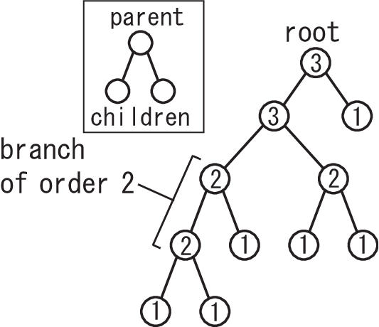
In order to derive topological characteristics of branching patterns, a method of branch ordering has been introduced by Horton [5] and Strahler [6]. With this method, ramification complexity and a hierarchical structure of branching patterns can be measured. For each node $v$ in a binary tree $T$, the Horton-Strahler index $S(v)$ is defined recursively as

where $\delta_{i,j}$ is the Kronecker delta. We define a branch of order $r$ as a maximal path connecting nodes of order $r$. The ratio of the number of branches of two subsequent orders is called the bifurcation ratio, and it has been found in many branching patterns that the bifurcation ratio takes almost constant value for different orders, which is known as “Horton’s law of stream numbers” especially in river networks [5]. Horton-Strahler analysis has been applied to a wide range of branching patterns [7, 8, 9, 10, 11, 12, 13, 14, 15].

A simple model called random model or equiprobable model, formulated by Shreve [16], is a finite probability space $(\Omega_{n},P_{n})$, where $\Omega_{n}$ denotes the sample space consisting of topologically distinct binary trees of magnitude $n$, and $P_{n}$ is the uniform probability measure on $\Omega_{n}$. We also introduce a random variable $S_{r,n}:\Omega_{n}\to\mathbb{N}\cup\{0\}$ such that $S_{r,n}(T)$ represents the number of branches of order $r$ in a binary tree $T\in\Omega_{n}$. Horton’s law on $(\Omega_{n},P_{n})$ is stated in the form

where $E(\cdot)$ denotes the average on $(\Omega_{n},P_{n})$, and $r=2,3,\cdots$. Analytical or combinatorial properties of $S_{r,n}$ are discussed in [17, 18, 19, 20, 21, 22, 23] for example.

Wang and Waymire analytically proved the central limit theorem

where “$\Rightarrow$” denotes convergence in distribution, and $N(\mu,\sigma^{2})$ denotes Gaussian distribution with mean $\mu$ and variance $\sigma^{2}$ [24]. Eq. (3) is equivalently expressed as

In the same way as Eq. (2), we expect the following relations

And, Eq. (3) is considered to be naturally generalized to

where $\sigma_{r}^{2}$ and $\tilde{\sigma}_{r}^{2}$ are variances depending on the order $r$. However, the proof of Eqs. (4) has not been performed analytically or numerically so far, and the values of $\sigma_{r}$ and $\tilde{\sigma}_{r}$ have not been obtained for $r\geq 3$. In the present paper, we propose a method of calculating Horton-Strahler indices of a binary tree by using binary sequence, and show numerical evidence for the validity of Eqs. (4).

A Dyck path of length $2(n-1)$ is a sequence of points $(s_{0},\cdots,s_{2(n-1)})$ on a two-dimensional lattice $\mathbb{Z}^{2}$ from $s_{0}=(0,0)$ to $s_{2(n-1)}=(n-1,n-1)$ such that each point $s_{i}=(x_{i},y_{i})$ satisfies $x_{i}\geq y_{i}$ and each elementary step $(s_{i},s_{i+1})$ is either rightward or upward (see Fig. 2).

For each Dyck path, a binary sequence of length $2(n-1)$ is generated by replacing a rightward step with ‘1’ and an upward step with ‘0’. The binary sequences generated by this replacement are formally called Dyck words on the alphabet $\{1,0\}$ [25], and for simplicity we call them Dyck sequences throughout the paper. Clearly, Dyck sequences share the two properties: (i) the total number of ‘0’ (and also ‘1’) is $n-1$, (ii) cumulative number of ‘0’ is never greater than that of ‘1’.

A correspondence between the Dyck paths of length $2(n-1)$ and the binary trees of magnitude $n$ is explained as follows (see Fig. 3 for reference). (i) Start with a Dyck path of length $2(n-1)$. (ii) Draw diagonal lines from upper right to lower left which are never below the Dyck path. (iii) Extract only the diagonals and the vertical lines in the Dyck path. It is found that the pattern obtained from this process is topologically the same as a binary tree of magnitude $n$, shown in Fig. 3 (b). Note that each Dyck path has one-to-one correspondence to a binary tree. Therefore, a Dyck path possesses the same topological structure as the corresponding binary tree.

The above method can be reformulated in a different way, where a Dyck sequence is generated from a binary tree. Here, a binary tree is regarded as a graph representing a successive merging process of two adjacent nodes, and each merging is expressed by putting two nodes in parentheses ‘$(\ )$’. Thus, the topological structure of a binary tree $T\in\Omega_{n}$ is fully expressed by a sequence of the leaves $v_{1},\cdots,v_{n}$ of $T$ and $n-1$ pairs of ‘$(\ )$’ [an example is shown as step (i) in Fig. 4]. A correspondence between a binary tree $T\in\Omega_{n}$ and a Dyck sequence of length $2(n-1)$ consists of the following two steps. (i) Convert $T$ into a sequence of $v_{1},\cdots,v_{n}$ and ‘$(\ )$’. (ii) Eliminate ‘$v_{1}$’ and ‘$($’, and replace $v_{2},\cdots,v_{n}$ with ‘$1$’ and ‘$)$’ with ‘$0$.’ A generated binary sequence proves to be a Dyck sequence and the correspondence is one-to-one. Fig. 4 illustrates this correspondence. Note that this process is similar to an expression tree and reverse Polish notation in formula manipulation [26].

The Horton-Strahler indices of a binary tree can be calculated through the corresponding Dyck sequence. The method consists of the following two steps: (i) Add ‘1’ to the top of the Dyck sequence. (ii) Replace a segment ‘$m\;n\;0$’ ($m,n>0$) with a single number ‘$\max\{m,n\}+\delta_{m,n}$’ recursively until the length of a sequence becomes 1. It is found that the number of times of a transformation ‘$(r-1)\;(r-1)\;0$’ $\to$ ‘$r$’ is identical with $S_{r,n}(T)$ for $r\geq 2$. Note that the operation (ii) is similar to Eq. (1) as shown in Fig. 5.

A basic method for generation of random Dyck paths is summarized in [27]. In this section, we present a method in a little different manner from [27]. We also propose a graphical representation for the generation process.

Let $\mathcal{D}$ denote the set of points in $\mathbb{Z}^{2}$ where at least one Dyck path passes, that is, $\mathcal{D}\equiv\{(x,y)\in\mathbb{Z}^{2}\mid 0\leq x,y\leq n-1,\ x\geq y\}$. We assign ‘transition probabilities’ $P_{\rightarrow}(x,y)$ and $P_{\uparrow}(x,y)$ on each point $(x,y)\in\mathcal{D}$. Each elementary step $(s_{i},s_{i+1})$ of a Dyck path $(s_{1},\cdots,s_{2(n-1)})$ is selected stochastically: stepping rightward with a probability $P_{\rightarrow}(s_{i})$ and upward with $P_{\uparrow}(s_{i})$. A set of transition probabilities yields a generation probability of a Dyck path $(s_{0},\cdots,s_{2(n-1)})$, which is given by

Since we focus on the random binary-tree model, we need to determine the transition probabilities where every Dyck path is generated equiprobably.

We define a monotonic path from $(x,y)\in\mathcal{D}$ as a sequence of points on $\mathcal{D}$ from $(x,y)$ to $(n-1,n-1)$ where each elementary step is either rightward or upward. Clearly, the length of a monotonic path from $(x,y)$ is $2(n-1)-(x+y)$, and a monotonic path from $(0,0)$ is identical with a Dyck path. The total number $N(x,y)$ of the monotonic paths from $(x,y)$ is written as

For the calculation of Eq. (5), we employed the reflection principle familiar in random-walk theory [28].

There are several remarks on $N(x,y)$:

1. 1.

   For any $(x,y)\in\mathcal{D}$, $N(x,y)$ is positive.

2. 2.

   $N(n-1,y)=1$, when $y=0,\cdots,n-1$.

3. 3.

   If $(x,y)$ is on the diagonal [i.e., $(x,y)=(k,k)$], then $N(k,k)=\frac{\{2(n-k-1)\}!}{(n-1-k)!(n-k)!}$, which is known as the $(n-k-1)$th Catalan number [29].

4. 4.

   The number of Dyck paths [which can be expressed as $N(0,0)$] is given by the $(n-1)$th Catalan number. This is well-known result, going back to Cayley [30].

5. 5.

   $N(x,y)=N(x+1,y)+N(x,y+1)$ for all $(x,y)\in\mathcal{D}$, where we set $N(x,y)=0$ if $(x,y)\not\in\mathcal{D}$.

On each point $(x,y)\in\mathcal{D}$, we define transition probabilities $P_{\rightarrow}(x,y)$ and $P_{\uparrow}(x,y)$ as

Specifically, $P_{\rightarrow}+P_{\uparrow}\equiv 1$, $P_{\uparrow}(k,k)=0$ and $P_{\rightarrow}(n-1,y)=0$. It is also proved inductively that Eqs. (6) realize random generation of Dyck paths.

Next, we propose a graphical representation of random Dyck paths. The number $N(x,y)$ can be calculated graphically as follows:

1. (i)

   Set $N(n-1,y)=1$ for all the rightmost points $(n-1,y)\;(y=0,\cdots,n-1)$ of $\mathcal{D}$. This implies that there is only one monotonic path from $(n-1,y)$, which is composed only of upward steps.

2. (ii)

   For convenience, let $N(x,y)=0$ for all $(x,y)\not\in\mathcal{D}$.

3. (iii)

   $N(x,y)$ is calculated from $N(x,y)=N(x+1,y)+N(x,y+1)$, that is, $N(x,y)$ is given by the sum of the value $N$ on the right and upper adjacent points [thus, $N(x,y)$ is calculated from right to left, top to bottom]. This implies that the monotonic paths from $(x,y)$ consist of ones passing through $(x+1,y)$ and $(x,y+1)$.

Note that $N(x,y)$ determined from (i)-(iii) is identical with Eq. (5). The graphical representation and examples of generation probability is depicted in Fig. 6. We can roughly confirm the uniformity of generated Dyck paths through successive canceling.

The Gaussian distribution function with mean $0$ and variance $\sigma^{2}$ is written as

where $\erf(x)$ is the error function defined as

Thus, the central limit theorems (4a) and (4b) are respectively rewritten as

A numerical algorithm for the calculation of $\sigma_{r}$ and $\tilde{\sigma}_{r}$ is summarized as follows:

1. (i)

   Generate Dyck sequences of length $2(n-1)$ randomly, on the basis of the method in Sec. 3.

2. (ii)

   Calculate Horton-Strahler indices of the Dyck sequences.

3. (iii)

   Compute values of both $\sqrt{n}\left(\frac{S_{r,n}}{S_{r-1,n}}-\frac{1}{4}\right)$ and $\sqrt{n}\left(\frac{S_{r,n}}{n}-\frac{1}{4^{r-1}}\right)$ for $r=2,3,\cdots$.

4. (iv)

   Make distribution functions from the values, then determine the values of $\sigma_{r}$ and $\tilde{\sigma}_{r}$ by fitting Eq. (7) to the distribution functions.

Fig. 7 shows distribution functions of $\sqrt{n}\left(\frac{S_{r,n}}{S_{r-1,n}}-\frac{1}{4}\right)$ and $\sqrt{n}\left(\frac{S_{r,n}}{n}-\frac{1}{4^{r-1}}\right)$ generated from $10^{5}$ samples with $n=10000$. The stepwise increases appear in the cases of $r=6$ and 7 in Fig. 7 (a), because the denominator $S_{r-1,n}$ of a fraction $\frac{S_{r,n}}{S_{r-1,n}}$ is decreasing with respect to $r$.

By fitting of the distribution function (7) to each data set in Fig. 7, we obtain Table 1 and Fig. 8 which suggest the relations

Eq. (9a) is good agreement with our numerical results. Eq. (9b) also seems to be consistent with our results, although there are errors of about a few percent ($\leq 4\%$) between $r$ and $-\log_{2}\tilde{\sigma}_{r}$.

In conclusion, the two central limit theorems are stated as

Note that both Eqs. (10) are reduced to Eq. (3) when $r=2$.

The Horton-Strahler index is based on ‘merging’ or ‘joining’ of branches in a binary tree, and a Dyck sequence generated from the method in Sec. 2 preserves a merging structure of the initial binary tree. Thus, the correspondence presented in this paper is suitable for the calculation of Horton-Strahler indices. It is known that there are some other ways of one-to-one correspondence between Dyck paths and binary trees [29, 31, 32]. However, Dyck paths generated from such other methods are not directly connected to the Horton-Strahler indices.

Our method can supply various numerical calculations based on the random binary-tree model, not only the central limit theorems. For example, see Fig. 9, our method is able to reproduce an asymptotic expansion of the bifurcation ratio

quite well, which has been obtained analytically by Moon [33]. Moreover, for systems other than the random model, we expect that our method is effective with some modification of transition probabilities.

Generation of random Dyck paths can be regarded as a Markov process on $\mathcal{D}$, which is called the Bernoulli excursion [34]. In addition, with taking a certain scaling limit, the Bernoulli excursion converges weakly to a diffusion process called the Brownian excursion [35], which is defined as one-dimensional Brownian motion $\{B(t):0\leq t\leq 1\}$ such that $P(B(0)=0)=P(B(1)=0)=1$ and $P(B(t)\geq 0)=1$ for $0\leq t\leq 1$. We expect that some asymptotic properties of the random binary-tree model are derived from the corresponding scaling limit.

Furthermore, the number $N(x,y)$ given by Eq. (5) is an example of the Kostka number, appearing in some combinatorial problems [36, 37]. It is expected that such other systems are related to a generation of random Dyck paths.

In the present paper, we propose a numerical method of generating random binary trees in the form of Dyck sequences. We also propose a method of calculating the Horton-Strahler indices from Dyck sequences. From numerical results, we confirm that the variances $\sigma_{r}$ and $\tilde{\sigma}_{r}$ are determined as Eqs. (9). Therefore, validity of the central limit theorems (10) are suggested numerically.

References

- [1] V. Fleury, J. -F. Gouyet, and M. Léonetti, Branching in Nature (Springer, Berlin, 2001).
- [2] P. Ball, The Self-made Tapestry (Oxford University Press, Oxford, 1999).
- [3] N. Wirth, Algorithms and Data Structures (Parentice Hall, 1986).
- [4] A. V. Aho, J. E. Hopcroft, and J. D. Ullman, Data Structures and Algorithms (Addison-Wesley Pub., 1983).
- [5] R. Horton, Bull. Geol. Soc. Am. 56, 275 (1945).
- [6] A. N. Strahler, Bull. Geol. Soc. Am. 63, 117 (1952).
- [7] M. Berry and P. M. Bradley, Brain Res. 109, 111 (1976).
- [8] K. N. Ganeshaiah and T. Veena, Behav. Ecol. Sociobiol. 29, 263 (1991).
- [9] G. M. Berntson, J. Theor. Biol. 177, 271 (1995).
- [10] J. Feder, E. L. Hinrichsen, K. J. Måløy, and T. Jøssang, Physica D 38, 104 (1989).
- [11] P. Ossadnik, Phys. Rev. A 45, 1958 (1991).
- [12] K. Horsfield, J. Theor. Biol. 87, 773 (1980).
- [13] X. G. Viennot, G. Eyrolles, N. Janey, and D. Arquès, Computer Graphics 23, 31 (1989).
- [14] J. Vannimenus and X. G. Viennot, J. Stat. Phys. 54, 1529 (1989).
- [15] I. Zaliapin, H. Wong, and A. Gabrielov, Tectonophysics, 413, 93 (2006).
- [16] R. L. Shreve, J. Geol. 74, 17 (1966).
- [17] C. Werner, Can. Geographer 16, 50 (1972).
- [18] A. Meir, J.W. Moon, and J. R. Pounder, SIAM J. Algebraic Discrete Methods 1, 25 (1980).
- [19] V. K. Gupta and E. Waymire, J. Hydrol. 65, 95 (1983).
- [20] L. Devroye and P. Kruszewski, Inf. Process. Lett. 56, 95 (1995).
- [21] H. Prodinger, Theor. Comput. Sci. 181, 181 (1997).
- [22] Z. Toroczkai, Phys. Rev. E 65, 016130 (2001).
- [23] K. Yamamoto and Y. Yamazaki, Phys. Rev. E 78, 021114 (2008).
- [24] S. X. Wang and E. C. Waymire, SIAM J. Discr. Math. 4, 575 (1991).
- [25] P. Duchon, Discr. Math. 225, 121 (2000).
- [26] T. Koshy, Discrete Mathematics with Applications (Academic Press, 2004).
- [27] L. Alonso and R. Schott, Random Generation of Trees : Random Generators in Computer Science (Springer, 1995).
- [28] A. F. Karr, Probability (Springer-Verlag, 1993).
- [29] J. H. Conway and R. K. Guy, The book of Numbers (Copernicus, 1996).
- [30] A. Cayley, Philosophical Magazine 28, 374 (1858).
- [31] L. Alonso and R. Schott, Theor. Comput. Sci. 159, 15 (1996).
- [32] X. G. Viennot, Discr. Math, 246, 317 (2002).
- [33] J. W. Moon, Ann. Discr. Math. 8, 117 (1980).
- [34] L. Takács, Adv. Appl. Prob. 23, 557 (1991).
- [35] I. I. Gikhman and A. V. Skorokhod, Introduction to the Theory of Random Processes (Courier Dover Pub., 1996).
- [36] I. G. Macdonald, Symmetric Functions and Hall Polynomials (Clarendon, Oxford, 1979).
- [37] R. P. Stanley, Enumerative combinatorics, vol. 2 (Cambridge University Press, 1999).