Solitons in quasi one-dimensional Bose-Einstein condensates with competing dipolar and local interactions
Abstract
We study families of one-dimensional matter-wave bright solitons supported by the competition of contact and dipole-dipole (DD) interactions of opposite signs. Soliton families are found, and their stability is investigated in the free space, and in the presence of an optical lattice (OL). Free-space solitons may exist with an arbitrarily weak local attraction if the strength of the DD repulsion is fixed. In the case of the DD attraction, solitons do not exist beyond a maximum value of the local-repulsion strength. In the system which includes the OL, a stability region for subfundamental solitons (SFSs) is found in the second finite bandgap. For the existence of gap solitons (GSs) under the attractive DD interaction, the contact repulsion must be strong enough. In the opposite case of the DD repulsion, GSs exist if the contact attraction is not too strong. Collisions between solitons in the free space are studied too. In the case of the local attraction, they merge or pass through each other at small and large velocities, respectively. In the presence of the local repulsion, slowly moving solitons bounce from each other.
pacs
03.75.Lm; 32.10.Dk; 05.45.YvI Introduction
Stable localized matter-wave structures in Bose-Einstein condensates (BECs) are supported by the interplay between the intrinsic nonlinearity, which is induced by collisions between atoms, quantum pressure, which originates from the kinetic energy of atoms, and external potentials [1]. This mechanism has made it possible to create bright solitons in condensates of 7Li and 85Rb atoms confined in cigar-shaped traps [2], where the inter-atomic interactions are made attractive by means of the Feshbach resonance (FR) [3]. In the condensate of 87Rb atoms with repulsive interactions, the introduction of an optical-lattice (OL) potential gives rise to gap solitons (GSs), as demonstrated experimentally in Ref. [4], see also review [5]. Dark solitons have been created too, by means of various techniques, in the self-repulsive 87Rb condensate [6]. In terms of the theoretical description, the limit case of a very deep OL may be mapped, by means of the tightly-binding approximation, into a discrete nonlinear Schrödinger equation and, accordingly, GSs are mapped into staggered discrete solitons [7].
New possibilities for the formation of matter-wave solitons are suggested by the presence of long-range interactions in dipolar condensates, which may be composed of magnetically polarized 52Cr atoms [8], dipolar molecules [9], or atoms in which electric moments are induced by a strong external field [10]. Solitons supported by the dipole-dipole (DD) interactions were predicted in two-dimensional (2D) settings. In the isotropic configuration, with moments fixed perpendicular to the plane, the natural DD interaction gives rise to repulsion, which can support delocalized states in the form of vortex lattices [11, 12]. In principle, the sign of the DD interaction in this configuration may be reversed by means of rapid rotation of the dipoles [13], suggesting a possibility to create isotropic solitons [14], as well as solitary vortices [12, 15]. On the other hand, stable anisotropic solitons have been predicted assuming the natural DD interaction between dipoles with a fixed in-plane polarization [16]. In addition to these results pertaining to the BEC context, it is relevant to mention that stable vortex rings were predicted in an optical model with the nonlocal thermal nonlinearity [17], and , elliptically shaped spatial solitons were created in such media experimentally [18].
Although one-dimensional (1D) configurations may be simpler than their 2D counterparts, 1D matter-wave bright solitons were not yet studied in detail in models of dipolar condensates, except for discrete solitons of the unstaggered type, which were recently predicted in the condensate trapped in a deep OL [19]. In those works, both attractive and repulsive signs of the onsite (contact) nonlinearity and long-range DD interactions between sites of the respective lattice were considered. The objective of the present work is the theoretical study of various types of bright solitons possible in the continuum BEC model featuring the competition between the contact and DD interactions. The effective strength of the DD interactions in the 1D geometry can be controlled by adjusting the orientation of the dipoles with respect to the axis of the linear trap, while the strength of the contact interactions may be effectively tuned by means of the FR technique, as shown in the condensate of 52Cr atoms [20]. The model is formulated both in the free space (i.e., in the absence of external potentials) and in the presence of the OL potential, which opens additional possibilities for the creation of stable localized states, including GSs (note that staggered discrete solitons, which, as mentioned above, correspond to GSs in the deep-OL limit, were not considered in Ref. [19]). In the framework of the Gross-Pitaevskii equation (GPE) with the ordinary local nonlinear term, the concept of GSs was elaborated in detail, see Refs. [21]-[23] and review [5]. However, to the best of our knowledge, it was not yet extended to the new physically relevant case, when the OL potential acts together with the long-range DD interaction – a situation that we address below.
The paper is organized as follows. The model is formulated in Section II, which, in Section III, is followed by the consideration of solitons supported by competing nonlinearities – attractive local/repulsive DD, or vice versa – in the free space. The model which combines the competing nonlinearities of both types and the OL is considered in Section IV. In that case, we report results for regular solitons in the semi-infinite gap, and for GSs in the two lowest finite bandgaps. In Section V, we deal with collisions between moving solitons in the absence of the OL. The paper is concluded by Section VI.
II The model
Our aim is to construct soliton states within the framework of the 1D GPE for the mean-field wave function, . The scaled equation includes the OL potential, (where is the strength of the OL, while its period is normalized to be ), the local nonlinear term with the respective coefficient, , and its nonlocal counterpart, with coefficient , which accounts for the DD interactions:
| (1) |
where subscripts denote partial derivatives. The kernel of the DD term was taken in two different ways, so as to avoid the divergence at . The first version relies on an explicit cut-off (CO kernel),
| (2) |
where is a constant. The other choice makes use of the regularized expression deduced in Ref. [24] by means of the single-mode approximation (SMA), i.e., the SMA kernel:
| (3) |
with being the standard complimentary error function. The two kernels are compared in Fig. 1. The most significant difference between them is that the SMA version features a cusp at , whereas the CO kernel has a smooth maximum. We have concluded that the choice of in CO expression (2), which makes areas beneath both curves equal, provides for the best proximity of the corresponding results to what has been found using the SMA approximation. Below, we report results obtained with the SMA kernel, as its CO counterpart yields virtually identical findings.

We fix the normalizations in Eq. (1) by setting , and then vary . In the the case of the 52Cr condensate, a characteristic value of the relative strength of the DD and contact interactions, which may be estimated as , is [20]; this value may be altered in broad limits by means of the FR technique. The interactions are repulsive or attractive for and , respectively. We will focus on the case of competing interactions, with , which is the most interesting one; in the case when both nonlinearities have the same sign, results turn out to be very similar to those reported previously in the local model. It is relevant to mention that, in terms of discrete systems, the competition of on-site (local) and inter-site (short-range nonlocal) interactions in 1D and 2D Salerno lattices were considered in Refs. [25] and [26], respectively. A number of stable discrete-soliton states which are impossible in the absence of the competition were reported in those works, including cuspons and peakons in 1D, and vortex breathers in 2D.
Stationary solutions to Eq. (1) with chemical potential are sought as . To construct such solutions, we discretize the resulting equation for by means of a finite-difference scheme, which leads to a set of coupled algebraic equations,
| (4) |
with , and . Solutions to Eq. (4) are sought by dint of the Newton-Raphson scheme. Results were obtained with a reasonable accuracy by choosing . To present soliton families, we will use norm and width of the soliton,
| (5) |
These definitions were adapted to the finite-difference form of the model as well.
Stability of the solutions was analyzed in the standard way (see, e.g., Ref. [27]), by considering a perturbation in the form of (where stands for complex conjugate). The linearized equations for the perturbation eigenmodes (i.e., the Bogoliubov - de Gennes equations) are written as
| (6) |
where we define
| (7) | |||||
| (8) |
| (9) |
The instability sets in when there emerges an eigenvalue with . Stability eigenvalues were obtained from a numerical solution of Eq. (6), by means of a standard eigenvalue solver from Fortran-based software package LAPACK [28].
III Solitons in the absence of the optical lattice
We start the presentation of results by considering the model with competing nonlinearities in the free space, i.e., with in Eq. (1). This implies that solitons may exist with .
III.1 Attractive local and repulsive nonlocal interactions
In accordance with what was said above, we first fix (the repulsive DD interaction), and vary negative (local attraction) and negative . In this case, solitons exist for every ; however, due to discretization, the numerical solution of Eq. (4), with the above-mentioned choice of , yields solitons in the region of . In fact, although very narrow solitons indeed exist at arbitrarily small values of , the soliton’s width becomes comparable to or smaller than this value of at , i.e., a better numerical accuracy is required to produce accurate soliton solutions in this range. Note that, for very narrow solitons with amplitude , the nonlinear part of Eq. (4), with , takes the form of . The existence of the soliton demands a negative coefficient in this expression, i.e.,
| (10) |
where it was taken into regard that , as per Eq. (3). In particular, for , condition (10) amounts to , as said above.
Figure 2(a) shows typical examples of the solitons in the present case, while Fig. 3 represents soliton families in terms of dependences and , for fixed values of and , respectively; note that plots in panel (b) of the latter figure are cut at , as the numerical accuracy is insufficient to extend them to smaller values of , as explained above. The stability of the solitons was verified both through the computation of the eigenvalues, using Eq. (6), and by means of direct simulations of the evolution of perturbed solitons. The well-known Vakhitov–Kolokolov criterion, [29], also suggests the stability of solitons in this case, although the negative slope of the curve in Fig. 3(a) is very small.
 |
 |
| (a) | (b) |
 |
 |
| (a) | (b) |
III.2 Repulsive local and attractive nonlocal interactions
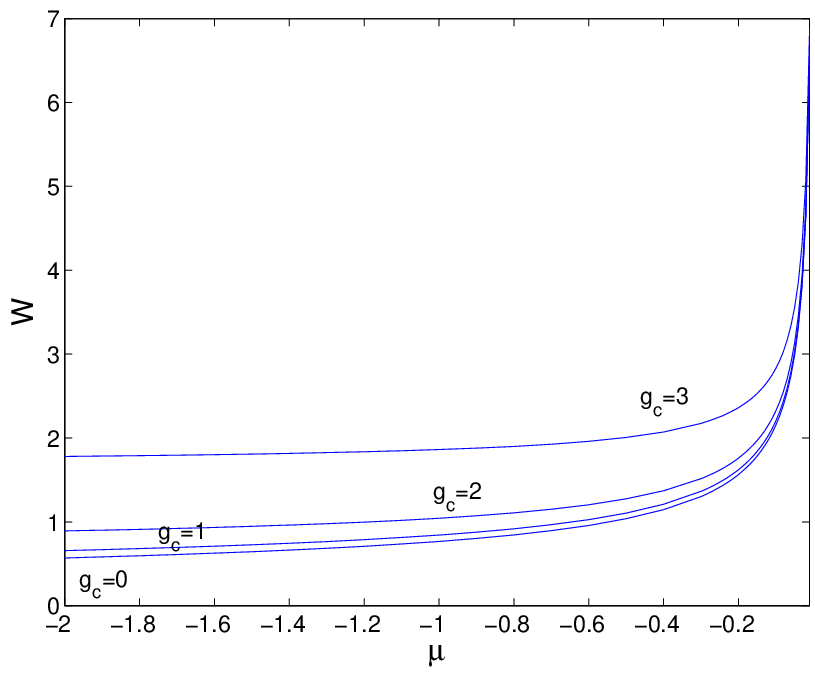
Now, we fix , varying and . Contrary to the previous case, solitons (which are stable) can be readily found for all values of up to , the difference between (zero local interaction, while the DD attraction is present) and amounting to a gradual increase of the soliton’s amplitude and width with . As seen in Fig. 2(b), close to the soliton develops a compacton-like shape, and solitons cannot be found at .
The existence of can be easily explained. Indeed, in the limit of and for a very broad soliton, the nonlinear part of Eq. (4), with , takes the approximate form of
| (11) |
The necessary condition for the existence of solitons is that the coefficient in front of in this expression must be negative [cf. the derivation of Eq. (10)], i.e.,
| (12) |
where expression (3) was used to perform the integration. For finite , the integral in expression (12) is replaced by . In particular, for , this yields , which is consistent with the above-mentioned numerical finding. Note also that the vanishing of the coefficient in front of in expression (11) at implies that the soliton’s amplitude and norm diverge in this limit, which is corroborated by the numerical results shown in Fig. 4.
 |
 |
The dependence of the soliton’s norm and width on the chemical potential is displayed in Fig. 5. Unlike the nearly flat dependences in Fig. 3, the present ones clearly satisfy the VK stability criterion, . The full stability of the solitons was confirmed by the computation of eigenvalues, using Eq. (6).
 |
 |
At this point, it is also worth to briefly consider dark solitons, which are known to be stable in BEC with contact repulsive interactions, such as 87Rb condensates [1, 6]. Dark solitons in three-dimensional dipolar BECs were recently considered in Ref. [30], where it was shown that, for sufficiently strong repulsive DD interactions and a sufficiently deep OL in the soliton’s nodal plane, dark solitons exist and are stable. In the present 1D setup, to investigate the existence and stability of dark solitons, it is first necessary to ensure that the respective background, namely, constant-amplitude state , is modulationally stable. A comprehensive analysis of the modulational instability (MI) of the background in the context of Eq. (1) can be performed following the lines of Ref. [31]. Here we will briefly consider this issue and provide an example of a stable dark soliton, assuming . In this case, the effective nonlinearity for long-wavelength perturbations (i.e., those with wave numbers ) is self-defocusing, i.e., the MI band cannot start at , as it does in the case of the standard nonlinear Schrödinger equation with the self-focusing nonlinearity. Although the MI band may appear at finite , this is not expected to happen as long as the background density is small enough, because the maximum MI gain is proportional to that density. Thus, in this case, a modulationally stable background may exist, and dark-soliton solutions can be found. As an example, in Fig. 6 we show a stable dark soliton (its stability was verified through the computation of the full spectrum of eigenvalues for small perturbations), which was found for and , . A systematic analysis of the MI of the background and dark-soliton families in the framework of Eq. (1) is beyond the scope of this work, and is deferred to a separate publication.

IV Solitons in the optical lattice
In the presence of the OL potential, generic results for regular solitons and gap solitons (GSs) in the model with the competing interactions can be adequately represented by fixing the OL strength to , which is adopted below. GSs have been found in the first and second finite bandgaps of the OL-induced linear spectrum. For , the two numerically computed (with ) bandgaps cover, respectively, the following intervals of the chemical potential:
| (13) |
IV.1 Attractive local and repulsive nonlocal interactions
Here, we consider solitons in the case of the competition between local attraction () and repulsive DD interactions (), varying and . The self-focusing character of the local interaction allows the existence of regular solitons in the semi-infinite gap, which is for . The numerical solution of Eq. (4), with , yields regular solitons for , similar to the case of , see above.
Apart from the solitons in the semi-infinite gap, GSs have been found in parts of the first and second finite bandgaps, for exceeding a certain critical value, which depends on , as shown in Fig. 7. Multi-humped solitons, which are bound states of fundamental single-humped solitons, can be found too. Numerical results demonstrate that the existence range for the multi-humped solitons is slightly broader than for the fundamental ones. In the second bandgap, single-humped solitons exist (and are stable) at . This boundary value, which corresponds to the vertical dashed line in Fig. 7, is located above the lower edge of the second bandgap, , see Eq. (13).

Another species of stable GSs was found in a part of the second finite bandgap, in the form of subfundamental solitons (SFSs). These are antisymmetric modes which are squeezed, essentially, into a single cell of the OL. The norm of the SFS is smaller than that of the fundamental GS, if the latter one can be found at the same value of (hence the name of “subfundamental” [32]). In a narrow interval adjacent to the lower edge of the second bandgap, , the SFSs are stable (see Fig. 7), whereas above this interval, they undergo a Hamiltonian-Hopf bifurcation, being unstable for smaller than a certain critical value. In the region of , SFSs are unstable in their entire existence region. In direct simulations, the destabilized SFSs spontaneously transform themselves into stable fundamental solitons belonging to the first (rather than second) bandgap; a similar scenario of the instability development of SFSs was found in the local model [32].
The existence regions for fundamental solitons (both regular ones in the semi-infinite gap and GSs in the first two finite bandgaps) and SFSs in the () plane are depicted together in Fig. 7; the existence region for multi-humped bound states is not shown separately, as it almost coincides with that of the fundamental solitons. In addition, Fig. 8 shows the norm as a function of at , for families of subfundamental and fundamental GSs, and for stable bound states of fundamental GSs [in the semi-infinite gap, the norm of all types of regular solitons very weakly depends on , cf. Fig. 3(a)]. Typical examples of solitons of all these types are displayed in Fig. 9. Bound states in the second finite bandgap are not shown, as they are completely unstable against oscillatory instabilities (while they are stable in the semi-infinite and first finite gaps). In fact, the same instability of bound states of GSs in the second finite bandgap occurs in the local model.

 |
 |
 |
 |
 |
 |
 |
 |
 |
 |
IV.2 Repulsive local and attractive nonlocal interactions
To adequately represent results in the model featuring the competition between the local repulsion () and DD attraction () in the model with the OL, it was sufficient to use a coarser numerical mesh, with (recall that was used above). The nonlocal self-attraction allows the existence of solitons in the semi-infinite gap. Similar to what was reported above for the same case in the free-space model, the solitons become very broad at approaching the critical value, . Other features of the regular solitons found in the semi-infinite gap are also similar to those of their free-space counterparts. The similarity holds also in the case of , i.e., in the model with the pure nonlocal attractive interactions.
The existence range for stable fundamental solitons (both the regular ones and GSs) and SFSs in the present version of the model is depicted in Fig. 10. Further, Fig. 11 shows the respective dependences, including those for bound-state solutions. This figure shows lines in the semi-infinite gap too, as, on the contrary to the situation for the model with and , these lines do not degenerate into . In fact, the opposite signs of for regular solitons and GSs is a typical feature, observed in local models as well. Typical profiles of various soliton species belonging to the semi-infinite and finite gaps are displayed in Fig. 12.

 |
 |
 |
 |
 |
 |
 |
 |
 |
 |
 |
 |
V Collisions between moving solitons
We have also studied collisions between solitons moving in the free space. In the model with the repulsive local and attractive DD interactions, a usual collision scenario is observed: at small velocities, solitons merge into a bound state, while, at high velocities, they pass through each other, as shown in Fig. 13.
 |
 |
| (a) | (b) |
The collision scenario is different in the opposite case, with the local attraction and nonlocal repulsion. As shown in Fig. 14, at small velocities the solitons bounce from each other. This feature is easily explained by the fact that the long-range interaction between the solitons is repulsive. The rebound is changed by the merger at intermediate values of the velocities. Finally, fast solitons pass through each other.
Dependences of critical values of collision velocities, which separate different outcomes of the collision, on the strength of the local interaction are displayed in Fig. 15.
 |
 |
| (a) | (b) |
In the presence of the OL, the solitons can be made mobile (by application of a kick to them) if the nonlinearity in the model is weak enough; otherwise, the respective Peierls–Nabarro is very high. In the weak-nonlinearity regime, the mobility of GSs in the present model is quite similar to that reported in the local model with the self-repulsive interactions [33], as well as in the discrete model including the DD interactions [19].
VI Conclusion
This work presents results of the systematic analysis of one-dimensional bright solitons supported by contact and dipole-dipole (DD) interactions of opposite signs in BEC. In the absence and in the presence of the optical lattice (OL), stable soliton families have been found for the cases of local attraction and DD repulsion or vice versa. In particular, free-space solitons can be supported by arbitrarily weak local attraction if the DD repulsion is fixed; in the opposite case, there is a maximum value of the strength of the local repulsion, beyond which solitons do not exist (which was explained in an analytical form). In the model including the OL, a notable finding is a region of stability of subfundamental solitons (SFSs) in the second finite bandgap. It is noteworthy too that, as seen in Figs. 10 and 7, the gap solitons (GSs) exist, in the case of the attractive DD interaction, if the contact repulsion is strong enough, and, in the opposite case of the repulsive DD interaction, GSs exist if the contact attraction is not too strong.
Collisions between bright solitons in the free space were considered too. The collision scenario is the usual one in the case of the local attraction (merger and quasi-elastic passage at small and large velocities, respectively), while in the opposite case, when the local interaction is repulsive, a region of rebound was additionally found at smallest values of the velocities, which is explained by the long-range repulsion between the solitons.
Acknowledgment
B.A.M. appreciate hospitality of the Nonlinear Physics Group of the University of Seville (Spain). The work of this author is supported, in a part, by grant No. 149/2006 from the German-Israel Foundation. P.G.K. gratefully acknowledges support from NSF-CARREER, NSF-DMS-0806762 and from the Alexander von Humboldt Foundation. The work of D.J.F. was partially supported by the Special Research Account of the University of Athens. J. C. acknowledges financial support from the Ministerio of Ciencia e Innovación of Spain, project number FIS2008-04848.
References
- [1] R. Carretero-González, D. J. Frantzeskakis, and P. G. Kevrekidis, Nonlinearity 21, R139 (2008).
- [2] K. E. Strecker, G. B. Partridge, A. G. Truscott, and R. G. Hulet Nature 417, 150 (2002); L. Khaykovich, F. Schreck, G. Ferrari, T. Bourdel, J. Cubizolles, L. D. Carr, Y. Castin, and C. Salomon, Science 296, 1290 (2002); S. L. Cornish, S. T. Thompson, and C. E. Wieman, Phys. Rev. Lett. 96, 170401 (2006).
- [3] S. Inouye, M. R. Andrews, J. Stenger, H.-J. Miesner D. M. Stamper-Kurn, and W. Ketterle, Nature (London) 392, 151 (1998); J. L. Roberts, N. R. Claussen, J. P. Burke, Jr., C. H. Greene, E. A. Cornell, and C. E. Wieman, Phys. Rev. Lett. 81, 5109 (1998); E. A. Donley, N. R. Claussen, S. L. Cornish, J. L. Roberts, E. A. Cornell, and C. E. Wieman, Nature (London) 412, 295 (2001).
- [4] B. Eiermann, Th. Anker, M. Albiez, M. Taglieber, P. Treutlein, K.-P. Marzlin, and M. K. Oberthaler, Phys. Rev. Lett. 92, 230401 (2004).
- [5] O. Morsch and M. K. Oberthaler, Rev. Mod. Phys. 78, 179 (2006); E. A. Ostrovskaya, M. Oberthaler, and Yu. S. Kivshar, in Emergent nonlinear phenomena in Bose-Einstein condensates. Theory and experiment, P. G. Kevrekidis, D. J. Frantzeskakis, and R. Carretero-González (eds.) (Springer, Heidelberg 2008).
- [6] S. Burger, K. Bongs, S. Dettmer, W. Ertmer, K. Sengstock, A. Sanpera, G. V. Shlyapnikov, and M. Lewenstein, Phys. Rev. Lett. 83, 5198 (1999); J. Denschlag, J. E. Simsarian, D. L. Feder, C. W. Clark, L. A. Collins, J. Cubizolles, L. Deng, E. W. Hagley, K. Helmerson, W. P. Reinhardt, S. L. Rolston, B. I. Schneider, and W. D. Phillips, Science 287, 97 (2000); A. Weller, J. P. Ronzheimer, C. Gross, J. Esteve, M. K. Oberthaler, D. J. Frantzeskakis, G. Theocharis and P. G. Kevrekidis, Phys. Rev. Lett. 101, 130401 (2008); C. Becker, S. Stellmer, P. Soltan-Panahi1, S. Döscher, M. Baumert, E.-M. Richter, J. Kronjäger, K. Bongs, and K. Sengstock, Nature Phys. 4, 496 (2008).
- [7] A. Trombettoni and A. Smerzi, Phys. Rev. Lett. 86, 2353 (2001); F. K. Abdullaev, B. B. Baizakov, S. A. Darmanyan, V. V. Konotop, and M. Salerno, Phys. Rev. A 64, 043606 (2001); G. L. Alfimov, P. G. Kevrekidis, V. V. Konotop, and M. Salerno, Phys. Rev. E 66, 046608 (2002).
- [8] A. Griesmaier, J. Werner, S. Hensler, J. Stuhler, and T. Pfau, Phys. Rev. Lett. 94, 160401 (2005); J. Stuhler, A. Griesmaier, T. Koch, M. Fattori, T. Pfau, S. Giovanazzi, P. Pedri, and L. Santos, ibid. 95, 150406 (2005); J. Werner, A. Griesmaier, S. Hensler, J. Stuhler, and T. Pfau, ibid. 94, 183201 (2005); A. Griesmaier, J. Stuhler, T. Koch, M. Fattori, T. Pfau, and S. Giovanazzi, ibid. 97, 250402 (2006); A. Griesmaier, J. Phys. B: At. Mol. Opt. Phys. 40, R91 (2007); T. Lahaye, T. Koch, B. Fröhlich, M. Fattori, J. Metz, A. Griesmaier, S. Giovanazzi, and T. Pfau, Nature (London) 448, 672 (2007).
- [9] T. Köhler, K. Góral, and P. S. Julienne, Rev. Mod. Phys. 78, 1311 (2006); J. Sage, S. Sainis, T. Bergeman, and D. DeMille, Phys. Rev. Lett. 94, 203001 (2005); C. Ospelkaus, L. Humbert, P. Ernst, K. Sengstock, and K. Bongs, ibid. 97, 120402 (2006); J. Deiglmayr, A. Grochola, M. Repp, K. Mörtlbauer, C. Glück, J. Lange, O. Dulieu, R. Wester, and M. Weidemüller, ibid. 101, 133004 (2008); F. Lang, K. Winkler, C. Strauss, R. Grimm, and J. H. Denschlag, ibid. 101, 133005 (2008).
- [10] M. Marinescu and L. You, Phys. Rev. Lett. 81, 4596 (1998); S. Giovanazzi, D. O’Dell, and G. Kurizki, Phys. Rev. Lett. 88, 130402 (2002); I. E. Mazets, D. H. J. O’Dell, G. Kurizki, N. Davidson, and W. P. Schleich, J. Phys. B 37, S155 (2004); R. Löw, R. Gati, J. Stuhler and T. Pfau, Europhys. Lett. 71, 214 (2005).
- [11] S. Yi and H. Pu, Phys. Rev. A 73, 061602(R) (2006).
- [12] V. M. Lashkin, Phys. Rev. A 75, 043607 (2007).
- [13] S. Giovanazzi, A. Görlitz, and T. Pfau, Phys. Rev. Lett. 89, 130401 (2002); A. Micheli, G. Pupillo, H. P. Büchler, and P. Zoller, Phys. Rev. A 76, 043604 (2007).
- [14] P. Pedri and L. Santos, Phys. Rev. Lett. 95, 200404 (2005); R. Nath, P. Pedri, and L. Santos, Phys. Rev. A 76, 013606 (2007); R. Nath, P. Pedri, and L. Santos, Phys. Rev. Lett. 102, 050401 (2009).
- [15] I. Tikhonenkov, B. A. Malomed, and A. Vardi, Phys. Rev. A 78, 043614 (2008).
- [16] I. Tikhonenkov, B. A. Malomed, and A. Vardi, Phys. Rev. Lett. 100, 090406 (2008).
- [17] D. Briedis, D. E. Petersen, D. Edmundson, W. Królikowski, and O. Bang, Opt. Exp. 13, 435 (2005).
- [18] C. Rotschild, O. Cohen, O. Manela, and M. Segev, Phys. Rev. Lett. 95, 213904 (2005).
- [19] G. Gligorić, A. Maluckov, Lj. Hadžievski, and B. A. Malomed, Phys. Rev. A 78, 063615 (2008); G. Gligorić, A. Maluckov, Lj. Hadžievski, and B. A. Malomed, Soliton stability and collapse in the discrete nonpolynomial Schrödinger equation with dipole-dipole interactions, Phys. Rev. A, in press.
- [20] T. Koch, T. Lahaye, J. Metz, B. Frölich, A. Griesmaier, and T. Pfau, Nature Phys. 4, 218 (2008).
- [21] F. Kh. Abdullaev, B. B. Baizakov, S. A. Darmanyan, V. V. Konotop, and M. Salerno, Phys. Rev. A 64, 043606 (2001); I. Carusotto, D. Embriaco, and G. C. La Rocca, ibid. 65, 053611 (2002); E. A. Ostrovskaya and Y. S. Kivshar, Phys. Rev. Lett. 90, 160407 (2003).
- [22] G. L. Alfimov, V. V. Konotop, and M. Salerno, Europhys. Lett. 58, 7 (2002); B. B. Baizakov, V. V. Konotop, and M. Salerno, J. Phys. B 35, 51015 (2002).
- [23] P. J. Y. Louis, E. A. Ostrovskaya, C. M. Savage, and Yu. S. Kivshar, Phys. Rev. A 67, 013602 (2003).
- [24] S. Sinha and L. Santos, Phys. Rev. Lett. 99, 140406 (2007).
- [25] J. Gomez-Gardeñes, B. A. Malomed, L. M. Floria, and A. R. Bishop, Phys. Rev. E 73, 036608 (2006).
- [26] J. Gomez-Gardeñes, B. A. Malomed, L. M. Floria, and A. R. Bishop, Phys. Rev. E 74, 036607 (2006).
- [27] D. E. Pelinovsky, A. A. Sukhorukov and Yu. S. Kivshar, Phys. Rev. E 70 036618 (2004).
- [28] A source of LAPACK is available at http://www.netlib.org/lapack/.
- [29] M. G. Vakhitov and A. A. Kolokolov, Sov. J. Radiophys. Quantum Electron. 16, 783 (1973); L. Bergé, Phys. Rep. 303, 260 (1998).
- [30] R. Nath, P. Pedri, and L. Santos, Phys. Rev. Lett. 101, 210402 (2008).
- [31] W. Królikowski, O. Bang, J. J. Rasmussen, and J. Wyller, Phys. Rev. E 64, 016612 (2001).
- [32] T. Mayteevarunyoo and B. A. Malomed, Phys. Rev. A 74, 033616 (2006).
- [33] H. Sakaguchi and B. A. Malomed. J. Phys. B: At. Mol. Opt. Phys. 37, 1443 (2004).