We consider decay of metastable topological configurations such as strings and domain walls. The transition from a state with higher energy density to a state with lower one proceeds through quantum tunneling or through thermally catalyzed quantum tunneling (at sufficiently small temperatures). The transition rate is calculated at zero temperature including the preexponential factor and also at a finite low temperature. The thermal catalysis factor is closely related to the probability (effective length) of destruction of the string (the domain wall) in collisions of the Goldstone bosons, corresponding to transverse waves on the string (wall). We derive a general formula which allows to find the probability (effective length) of a string (wall) breakup by a collision of arbitrary number of the bosons. We find that the destruction of a string only takes place in collisions of even number of the bosons, while the destruction of the wall can occur in a collision of any number of particles. We explicitly calculate the energy dependence of such processes in two-particle collisions for arbitrary relation between the energy and the largest infrared scale (the size of a critical gap).

1 Introduction

Topological configurations of fields with the geometry of a string or a domain wall arise in various models either as solutions of classical field equations or as nonperturbative effective configurations of essentially quantum fields. String-like configurations are present in polymers, superconductors, in theoretical models of non-Abelian dynamics, as well as in models of QCD confinement, and as topological defects in models with spontaneous breaking of gauge or global symmetries. Metastable domain wall solutions arise in models with spontaneously broken approximate symmetry. The existence of such solutions was shown from different points of view, for example, in Refs. [1, 2, 3].

These configurations are classically stable, since there is no classical trajectory which takes from one topological solution into another with different topological number. But it may be the case that a classically forbidden trajectory for such a deformation exists so that the considered configurations are unstable quasiclassically and decay due to e.g. quantum tunneling effects. As an illustration of such decay process one can consider the example of a metastable domain wall investigated in Refs. [4, 5] which arises in a model with a scalar field potential shown in Fig.1. The domain wall solution corresponds to the interpolation between the same vacuum state at two spatial infinities, e.g. at $z=-\infty$ and $z=+\infty$ with the field winding around the ‘peg’ in the potential.

Such configuration is classically stable in the sense that the solution with certain winding number can not evolve classically to a solution with different topological number. However, such a transition can proceed either due to a thermal fluctuation, where the path, corresponding to the solution, is lifted over the barrier or due to quantum tunneling (the motion in a classically forbidden region).

The topological configurations can be metastable with respect to either a complete breaking, or a transition to an object of lower tension emerging instead of the initial one. The former situation is relevant e.g. for a break up of a QCD string with formation of a quark - antiquark pair, or a formation of a monopole - antimonopole pair[6], and also in a whole class of theories with spontaneous symmetry breaking[7]. The latter situation involving a phase transition between states of a string with different tension is found e.g. in Abelian Higgs models embedded in non-Abelian theories [8, 9].

A domain wall decay is analogous to the well-known spontaneous false vacuum decay process [10, 11, 12] in $2+1$ dimensions. Indeed, if a hole of area $\mathcal{A}_{c}$ is created in a wall with tension $\epsilon$ , the gain in the energy is $\epsilon\,\mathcal{A}_{c}$ . The barrier that inhibits the process is created by the energy $\sigma\mathcal{P}$ , with $\mathcal{P}$ being the perimeter of the hole and $\sigma$ being a tension associated with the interface. Thus, the ‘area’ energy gain exceeds the barrier energy only starting from a critical size of the hole created, i.e. starting with a round hole of radius $R_{w}=2\sigma/\epsilon$ . Once a critical bubble of the lower phase has nucleated due to tunneling, it expands, converting the domain wall. Therefore the probability of the transition is given by the rate of nucleation of the critical holes in the domain wall.

The same argument also applies to the string decay which is similar to a metastable vacuum decay process in $1+1$ dimensions. The critical size of the gap in the initial string is then $\ell_{c}=2R_{s}=2\,\mu/\varepsilon$ . Moreover due to the geometry of the problem such decay also bears a great similarity to the well known Schwinger process of production of pair of charged particles by an external electromagnetic field [13].

Despite the similarity with the false vacuum decay the breaking of the strings and walls involves an essential difference associated with the transverse waves propagating on the latter objects, corresponding to massless bosons, which in fact are the Goldstone bosons of the spontaneously broken translational invariance. The effect of the soft modes of the field of these bosons enters the probability of breaking the topological defects at the preexponential level [5, 9].

The process of a metastable string transition from a state with tension $\varepsilon_{1}$ to a state with tension $\varepsilon_{2}$ was considered in [6, 7, 8]. Using the analogy with the false vacuum decay the decay rate was found with exponential accuracy in terms of the rate of nucleation of critical gaps per unit length of the string, $\gamma_{s}={d\Gamma/d\ell}$ ¹¹ 1 It should be mentioned that in $d=2$ there is no transverse motion for the string, and the preexponential factor can be also copied from the known result of spontaneous metastable vacuum decay $C_{d=2}={\varepsilon_{1}-\varepsilon_{2}\over 2\pi}~.$ ,

\gamma_{s}=C\,\exp\left(-\,{\pi\,\mu^{2}\over\varepsilon_{1}-\varepsilon_{2}}\right)~,

(1)

where $\mu$ is the mass associated with the interface between the two phases of the string. The decay rate of an axion domain wall was considered at the level of the semiclassical exponent in Ref. [4] by adapting the expression for metastable vacuum decay in $2+1$ dimensions.

The preexponential factors for the spontaneous decay of string and walls were calculated in [5, 9]. For a string the rate of the transition between the states with tension $\varepsilon_{1}$ and $\varepsilon_{2}$ was found to be

\gamma_{s}={\varepsilon_{1}-\varepsilon_{2}\over 2\pi}\,\left[F\left({\varepsilon_{2}\over\varepsilon_{1}}\right)\right]^{d-2}\,\exp\left(-\,{\pi\,\mu_{R}^{2}\over\varepsilon_{1}-\varepsilon_{2}}\right)~,

(2)

with the dimensionless factor $F$ given by

F\left({\varepsilon_{2}\over\varepsilon_{1}}\right)=\sqrt{\varepsilon_{1}+\varepsilon_{2}\over 2\,\varepsilon_{1}}\,\,{\rm\Gamma}\!\left({\varepsilon_{1}+\varepsilon_{2}\over\varepsilon_{1}-\varepsilon_{2}}+1\right)\,\left({\varepsilon_{1}-\varepsilon_{2}\over\varepsilon_{1}+\varepsilon_{2}}\right)^{\varepsilon_{1}+\varepsilon_{2}\over\varepsilon_{1}-\varepsilon_{2}}\,\exp\left({\varepsilon_{1}+\varepsilon_{2}\over\varepsilon_{1}-\varepsilon_{2}}\right)\left(2\pi\,{\varepsilon_{1}+\varepsilon_{2}\over\varepsilon_{1}-\varepsilon_{2}}\right)^{-1/2}~,

(3)

while the decay rate of a domain wall is formulated in terms of the rate $\gamma_{w}$ of nucleation of critical holes per unit area, $\gamma_{w}={d\Gamma/dA}$ ,

\gamma_{w}=\frac{\tilde{\mathcal{C}}}{\epsilon^{7/3}}\,\exp\left(-{16\,\pi\,\sigma_{R}^{3}\over 3\,\epsilon^{2}}\right)~,

(4)

where $\mu_{R}$ and $\sigma_{R}$ are renormalized mass and tension parameters associated with the interface of the strings and domain walls respectively, and $\tilde{\mathcal{C}}$ is a constant that does not depend on $\epsilon$ but does depend on other dimensional parameters in the underlying field theory.

The thermal effects in the decay of metastable strings [14] further expose the difference from the false vacuum decay and the Schwinger process. Namely, as long as the temperature $T$ is lower than the inverse of the critical length, $T<1/\ell_{c}$ the thermal effects in the latter processes are exponentially suppressed as $\exp(-m/T)$ with $m$ being the lowest scale for particle masses in the theory, and these effects are very small due to the strongly suppressed presence of massive particles in the thermal equilibrium[15]. In the case of a string, however, the transverse waves on the string are massless so that their excitation has no suppression by the mass at arbitrarily low temperature. The thermal excitations of these waves create fluctuations in the distribution of the energy in the string which catalyze the nucleation of the critical gap. Clearly, at $T\ll 1/\ell_{c}$ the typical wavelength of the thermal waves $\sim 1/T$ is large in comparison with the critical length $\ell_{c}$ , and the thermal effect in the rate is quite small, although not exponentially small. The leading low temperature correction in the nucleation rate is given by the thermal catalysis factor[14]

\mathcal{K}_{s}=1+(d-2)\,{\pi^{8}\over 450}\,\left({\varepsilon_{1}-\varepsilon_{2}\over 3\varepsilon_{1}-\varepsilon_{2}}\right)^{2}\,\left(\frac{\ell_{c}T}{2}\right)^{8}+O\left[(\ell_{c}T)^{12}\right]~,

(5)

while as $T$ approaches $1/\ell_{c}$ , the catalysis factor develops a singularity at $\ell_{c}T=1$ . At still higher temperatures the considered string transition behaves, in a sense, similarly to the false vacuum decay[15], namely the regime of the transition changes to a different tunneling trajectory, so that the temperature dependence appears in the semiclassical exponential factor in Eq.(2), rather than in the preexponential term.

The effect of the thermally excited waves in the decay rate can in fact be considered [16] as an additional contribution to the probability of the decay due to collisions of the Goldstone bosons that are present in the thermal bath. As it turns out, it is possible to identify in the thermal catalysis factor the contribution of individual such collisions and thus calculate the probability of the destruction of metastable string by colliding particles. In particular, the first temperature dependent term in the expansion (5) is entirely due to the process of the critical gap creation in a collision of two particles in the limit, where their center of mass energy $E=\sqrt{s}$ is much smaller than $1/\ell_{c}$ . In order to separate the terms in the decay probability originating from collisions of different number of the bosons, the standard thermal approach to calculating the decay rate at finite temperature [14] is modified [16] by formally introducing a negative chemical potential for the bosons. This allows to find the dependence of the probability of string destruction in an $n$ -boson collision for an arbitrary relation between $\ell_{c}$ and the energy of the bosons. One of the results of such a consideration is that the string destruction takes place only in collisions of even number of bosons and is absent at odd $n$ . The explicit expression for the (dimensionless) probability $W_{2}$ of the critical gap creation in two-boson collisions at arbitrary values of the parameter $E\,\ell_{c}$ has especially simple form for the decay of the string into ‘nothing’ i.e. at $\varepsilon_{2}=0$ :

W_{2}=2\,\pi^{2}\,\ell_{c}^{2}\,\gamma_{s}\,\left[I_{3}\left({E\ell_{c}\over 2}\right)\right]^{2}~,

(6)

with $I_{3}(x)$ being the standard notation for the modified Bessel function of the third order. This expression is applicable as long as the energy $E$ is small in comparison with the string energy scale: $E\ll\sqrt{\epsilon}$ , which condition still allows for the parameter $E\,\ell_{c}$ to be large. At $E\,\ell_{c}\gg 1$ the energy dependent factor in Eq.(6) has the exponential behavior $\exp(E\ell_{c})$ which matches the semiclassical approximation for the energy-dependent factor[17], corresponding to tunneling at the energy $E$ rather than at zero energy. In this sense the discussed energy dependence of the collision-induced probability of the decay describes the onset of the semiclassical behavior.

One can also notice that the thermal factor $\mathcal{K}_{s}$ , is singular [14] at $\ell_{c}T=1$ . However the two-boson production rate does not exhibit any singularity at any value of the parameter $E\ell_{c}$ , and a similar smooth energy behavior is also true for individual $n$ -boson processes. Thus the ‘explosion’ of the thermal rate at $\ell_{c}T=1$ is a result of infinite number of processes becoming important at this point, rather than due to a finite set of processes with a limited range of $n$ developing large probability at the energy per particle of the order of $1/\ell_{c}$ .

The purpose of this paper is to generalize to the case of a metastable domain wall the approach used for analyzing the thermal and collision induced effects in the decay of metastable strings. We find the general expression for the thermal catalysis factor $\mathcal{K}_{w}$ . In particular, the leading term in this factor at low temperature (in $d$ dimensions) is given by

\mathcal{K}_{w}=1+12\,(d-3)\,\zeta^{2}(5)\,(R_{w}\,T)^{10}+\dots.

(7)

where $R_{w}$ is the radius of the critical hole in the metastable wall, and $\zeta(x)$ is the standard notation for the Riemann $\zeta$ function, $\zeta(5)\approx 1.037$ . We also aim at providing here a systematic and self-contained presentation of the calculations leading to our final results. To this end we recapitulate in detail in Section 2 the technically simpler calculations for the processes with metastable strings, and then in Section 3 expand the method to the case of a metastable domain wall. Such ‘semi-review’ format of the paper also allows us to illustrate the similarity and the difference between the string and the domain wall transitions. Although the calculations in both cases are very much similar, the results differ in some essential details. In particular the destruction of a metastable wall is induced by a collision of any number of Goldstone bosons, whereas a string can be destroyed by a collision of only even number of the bosons. Another difference relates to the thermal catalysis of the decay: for a string the low temperature expansion for the enhancement of the quantum tunneling is applicable everywhere where the series is convergent, i.e. up to the temperature $T=1/\ell_{c}$ , while for a domain wall the thermal fluctuations start dominating[15] at a lower temperature ( $T=3/(4\ell_{w})$ with $\ell_{w}$ being the diameter of the critical hole in the wall), at which the thermal effects in the quantum tunneling probability are still very small numerically.

2 String-like configuration

2.1 Spontaneous decay of a metastable string

The tunneling trajectory can be described in the Euclidean space by a configuration called the ‘bounce’[11], which is a solution to (Euclidean) classical equations of motion. The general expression for the effective Euclidean space action for the string with the two considered phases can be written in the familiar Nambu-Goto form:

S=\mu\,P+\varepsilon_{1}\,A_{1}+\varepsilon_{2}\,A_{2}~,

(8)

where $A_{1}$ and $A_{2}$ are the areas of the world sheet for the two phases, and $P$ (the perimeter) is the length of the world line for the interface between them.

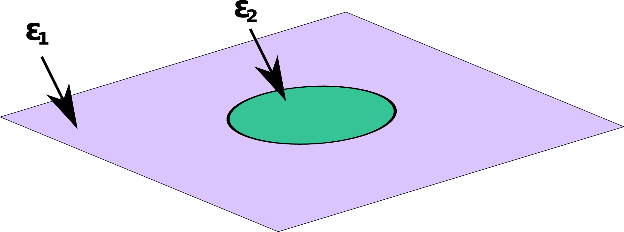
The action (8) is an effective low-energy expression in the sense that it only describes the ‘stringy’ variables and is applicable as long as the effects of thickness of the string and of its internal structure can be neglected. Denoting $M_{0}$ the mass scale at which such approach becomes invalid (e.g. the thickness of the string $r_{0}\sim 1/M_{0}$ ), one can write the condition for the applicability of the effective action (8) in terms of the length scale, $\ell\gg 1/M_{0}$ , and the momentum scale $k\ll M_{0}$ . Assuming that the initial very long string with tension $\varepsilon_{1}$ is located along the $x$ axis, one can readily find that the action (8) has a nontrivial stationary configuration, the bounce, namely, that of a disk in the (t,x) plane occupied by the phase $2$ , as shown in Figure 2, with the radius

R_{s}={\mu\over\varepsilon_{1}-\varepsilon_{2}}~,

(9)

which is the radius (one half of the length $\ell_{c}$ ) of the critical gap. The difference between the action (8) on this configuration and on the trivial one is exactly the expression for the exponential power in Eq.(1), and the condition for applicability of the effective action (8) requires

M_{0}\,R_{s}={M_{0}\,\mu\over\varepsilon_{1}-\varepsilon_{2}}\gg 1~.

(10)

Generally one also has $\mu\raisebox{-2.58334pt}{$\stackrel{{\scriptstyle\textstyle>}}{{\sim}}$}M_{0}$ , and for the strings in weakly coupled theories $\mu\gg M_{0}$ , so that the power in the exponent in Eq.(1) is large, which justifies a semiclassical treatment.

The probability of the transition is determined[11, 18, 19] by (the imaginary part of) the ratio of the path integrals ${\cal Z}_{12}$ and ${\cal Z}_{1}$ calculated with the action (8) around respectively the bounce configuration and around the initial flat string:

\gamma_{s}={1\over A}\,\mathrm{Im}\frac{{\cal Z}_{12}}{{\cal Z}_{1}}~.

(11)

It can also be reminded that, as explained in great detail in Ref.[18], that the imaginary part of ${\cal Z}_{12}$ arises from one negative mode at the bounce configuration, and that due to two translational zero modes the numerator in Eq.(11) is proportional to the total space time area $A$ in the $(t,x)$ plane occupied by the string, so that the finite quantity is the transition probability per unit time (the rate) and per unit length of the string.

In order to evaluate the relevant path integrals with pre-exponential accuracy we use the cylindrical coordinates, with $r$ and $\theta$ being the polar variables in the $(t,x)$ plane (of the bounce), and $z$ being the transverse coordinate. We consider only one transverse coordinate, since the effect of each of the extra dimensions factorizes, so that the corresponding generalization is straightforward. We further assume, for definiteness, that the space-time boundary in the $(t,x)$ plane is a circle of large radius $L$ , where the boundary condition for the string is $z(r=L)=0$ . The small deviations of the string configuration from the bounce, illustrated in Fig.3, can be parametrized by the radial ( $f$ ) and transverse ( $\xi$ ) shifts of the boundary between the string phases:

r(\theta)=R_{s}+f(\theta)\,,~~~~z(\theta)=\xi(\theta)~,

(12)

and by the variations of the surfaces of the two string phases: $z_{1}(r,\theta)$ and $z_{2}(r,\theta)$ , where, naturally,

z_{1}(R_{s},\theta)=z_{2}(R_{s},\theta)=\xi(\theta)~.

(13)

In terms of these variables the action (8) can be written in the quadratic approximation in the deviations from the bounce as

	$\displaystyle S_{12}=\varepsilon_{1}\,\pi\,L^{2}+{\pi\,\mu^{2}\over\varepsilon_{1}-\varepsilon_{2}}+{\varepsilon_{1}-\varepsilon_{2}\over 2}\,\int d\theta\,\left(\dot{\xi}^{2}+\dot{f}^{2}-f^{2}\right)+$
	$\displaystyle{\varepsilon_{1}\over 2}\,\int_{R_{s}}^{L}rdrd\theta\,\left(z_{1}^{\prime}\,{}^{2}+{\dot{z_{1}}^{2}\over r^{2}}\right)+{\varepsilon_{2}\over 2}\,\int_{0}^{R_{s}}rdrd\theta\,\left(z_{2}^{\prime}\,{}^{2}+{\dot{z_{2}}^{2}\over r^{2}}\right)~,$		(14)

where the primed and dotted symbols stand for the derivatives with respect to $r$ and $\theta$ correspondingly.

Finally, the action around a flat initial string configuration in the quadratic approximation takes the form

S_{1}=\varepsilon_{1}\,\pi L^{2}+{\varepsilon_{1}\over 2}\,\int_{0}^{L}rdrd\theta\,\left(z^{\prime}\,{}^{2}+{\dot{z}^{2}\over r^{2}}\right)~,

(15)

with $z(r,\theta)$ parametrizing small deviations of the string in the transverse direction.

2.1.1 Separating variables in the path integrals

One can readily see that in the quadratic part of the action (14) the ‘longitudinal’ variation of the bounce boundary in the $(t,x)$ plane, described by the function $f(\theta)$ completely decouples from the rest of the variables. This implies that the path integral over $f$ can be considered independently of the integration over other variables and that it enters as a factor in ${\cal Z}_{12}$ . On the other hand it is this integral that provides the imaginary part to the partition function, and it is also proportional to the total space-time area $A$ . Moreover, this path integral is identical to the one entering the problem of false vacuum decay in (1+1) dimensions and we can directly apply the result of that calculation[20]:

{1\over A}\,\mathrm{Im}\int{\cal D}f\,\exp\left[-{\varepsilon_{1}-\varepsilon_{2}\over 2}\,\int_{0}^{2\pi}\,\left(\dot{f}^{2}-f^{2}\right)\,d\theta\right]={\varepsilon_{1}-\varepsilon_{2}\over 2\pi}~.

(16)

The expression for the transition rate thus can be written in the form

{d\Gamma\over d\ell}={\varepsilon_{1}-\varepsilon_{2}\over 2\pi}\,\exp\left(-{\pi\,\mu^{2}\over\varepsilon_{1}-\varepsilon_{2}}\right)\,\,{{\tilde{\cal Z}}_{12}\over{\cal Z}_{1}}~,

(17)

with the path integral ${\tilde{\cal Z}}_{12}$ running only over the transverse variables $\xi$ , $z_{1}$ and $z_{2}$ ,

{\tilde{\cal Z}}_{12}=\int{\cal D}\xi\,{\cal D}z_{1}\,{\cal D}z_{2}\,\exp\left(-{\tilde{S}}_{12}\right)

(18)

and involving only the quadratic in these variables part of the action (14),

{\tilde{S}}_{12}={\varepsilon_{1}-\varepsilon_{2}\over 2}\,\int d\theta\,\dot{\xi}^{2}+{\varepsilon_{1}\over 2}\,\int_{R_{s}}^{L}rdrd\theta\,\left(z_{1}^{\prime}\,{}^{2}+{\dot{z_{1}}^{2}\over r^{2}}\right)+{\varepsilon_{2}\over 2}\,\int_{0}^{R_{s}}rdrd\theta\,\left(z_{2}^{\prime}\,{}^{2}+{\dot{z_{2}}^{2}\over r^{2}}\right)~.

(19)

In the same quadratic approximation the flat string partition function ${\cal Z}_{1}$ is given by

{\cal Z}_{1}=\int{\cal D}z\,\exp\left(-S_{1}\right)

(20)

with $S_{1}$ given by Eq.(15) and the integral running over all the functions vanishing at the space-time boundary: $z(L,\theta)=0$ .

At this point there still is a coupling in the path integral (18) between the bulk variables $z_{1}$ , $z_{2}$ and the boundary variable $\xi$ arising from the boundary conditions (13). This however is a simple issue which is resolved by a straightforward shift of the integration variables $z_{1}$ and $z_{2}$ . Namely, we write

z_{1}(r,\theta)=z_{1c}(r,\theta)+z_{1q}(r,\theta)~,~~~~z_{2}(r,\theta)=z_{2c}(r,\theta)+z_{2q}(r,\theta)~,

(21)

where $z_{1q}$ and $z_{2q}$ are the new integration variables in ${\tilde{\cal Z}}_{12}$ and these functions satisfy zero boundary conditions,

z_{1q}(R_{s},\theta)=z_{2q}(R_{s},\theta)=z_{1q}(L,\theta)=z_{2q}(L,\theta)=0~,

(22)

while $z_{1c}$ and $z_{2c}$ are fixed (for a fixed $\xi(\theta)$ ) functions satisfying the boundary conditions

z_{1c}(R_{s},\theta)=z_{2c}(R_{s},\theta)=\xi(\theta)~,z_{1c}(L,\theta)=0~,

(23)

which are also harmonic, i.e. satisfying the Laplace equation $\Delta z=0$ .

After the specified shift of the variables we arrive at the expression for the action (19) in which the bulk and the boundary degrees of freedom are fully separated:

	$\displaystyle{\tilde{S}}_{12}$	$\displaystyle=$	$\displaystyle{\varepsilon_{1}-\varepsilon_{2}\over 2}\,\int d\theta\,\dot{\xi}^{2}+R_{s}\,\int d\theta\,\left({\varepsilon_{2}\over 2}{\partial_{r}}z_{2c}\left.\right\|_{r=R_{s}}-{\varepsilon_{1}\over 2}{\partial_{r}}z_{1c}\left.\right\|_{r=R_{s}}\right)\,\xi$		(24)
		$\displaystyle-$	$\displaystyle{\varepsilon_{1}\over 2}\,\int d^{2}r\,z_{1q}\Delta z_{1q}-{\varepsilon_{2}\over 2}\,\int d^{2}r\,z_{2q}\Delta z_{2q}~.$		(24)

Clearly, the boundary terms in the first line here, arising from the integration by parts, depend only on the transverse shift of the boundary $\xi(\theta)$ . The partition function ${\tilde{\cal Z}}_{12}$ can thus be written as a product of the ‘boundary’ and the ‘bulk’ terms:

{\tilde{\cal Z}}_{12}={\cal Z}_{12(\rm boundary)}\,{\cal Z}_{12(\rm bulk)}~,

(25)

with the ${\cal Z}_{12(\rm bulk)}$ being given by the path integral over the bulk variables $z_{1q}$ and $z_{2q}$ only :

{\cal Z}_{12(\rm bulk)}=\int{\cal D}z_{1q}\,{\cal D}z_{q}\,\exp\left({\varepsilon_{1}\over 2}\,\int d^{2}r\,z_{1q}\Delta z_{1q}+{\varepsilon_{2}\over 2}\,\int d^{2}r\,z_{2q}\Delta z_{2q}\right)~,

(26)

and the boundary term

{\cal Z}_{12(\rm boundary)}=\int{\cal D}\xi\,\exp\left[-{\varepsilon_{1}-\varepsilon_{2}\over 2}\,\int d\theta\,\dot{\xi}^{2}-R_{s}\,\int d\theta\,\left({\varepsilon_{2}\over 2}{\partial_{r}}z_{2c}\left.\right|_{r=R_{s}}-{\varepsilon_{1}\over 2}{\partial_{r}}z_{1c}\left.\right|_{r=R_{s}}\right)\,\xi\right]

(27)

involving integration over only the boundary values.

The subsequent calculation of the ratio of the partition functions in Eq.(17) can in fact be reduced to a calculation of ${\cal Z}_{12(\rm boundary)}$ only. In order to achieve this reduction one should organize the partition function ${\cal Z}_{1}$ in the denominator of Eq.(17) in a form similar to Eq.(25) as follows. Although the flat string configuration makes no reference to a circle of the radius $R$ , the partition function ${\cal Z}_{1}$ can be calculated by first fixing the transverse variable $z$ at $r=R_{s}$ : $z(R_{s},\theta)=\xi(\theta)$ and separating the integration over the bulk variables. Then the flat string partition function factorizes in the form similar to Eq.(25):

{\tilde{\cal Z}}_{1}={\cal Z}_{1(\rm boundary)}\,{\cal Z}_{1(\rm bulk)}~,

(28)

with ${\cal Z}_{1(\rm bulk)}$ given a similar path integral as in Eq.(26),

{\cal Z}_{1(\rm bulk)}=\int{\cal D}z_{1q}\,{\cal D}z_{q}\,\exp\left({\varepsilon_{1}\over 2}\,\int d^{2}r\,z_{1q}\Delta z_{1q}+{\varepsilon_{1}\over 2}\,\int d^{2}r\,z_{2q}\Delta z_{2q}\right)~,

(29)

where, as in Eq.(26), $z_{1q}$ and $z_{2q}$ are respectively the outer (i.e. at $r>R_{s}$ ) and the inner ( $r<R_{s}$ ) transverse fluctuations with zero boundary conditions. The difference in the coefficient in the expressions (26) and (29) for the contribution of the inner part, $\varepsilon_{2}$ vs. $\varepsilon_{1}$ , is not essential, since the overall coefficient of the quadratic part of the action is absorbed in the measure of integration, as can be seen by rescaling to the corresponding canonically normalized variables $\phi=\sqrt{\varepsilon}\,z$ .

One therefore finds that ${\cal Z}_{1(\rm bulk)}={\cal Z}_{12(\rm bulk)}$ , and the ratio of the partition functions in Eq.(17) is in fact determined by the ratio of the boundary terms.

2.1.2 Regularization

The boundary factor ${\cal Z}_{1(\rm boundary)}$ for the flat string is somewhat different from the one given by Eq.(27) and reads as

{\cal Z}_{1(\rm boundary)}=\int{\cal D}\xi\,\exp\left[-R_{s}\,{\varepsilon_{1}\over 2}\,\int d\theta\,\left({\partial_{r}}z_{2c}\left.\right|_{r=R_{s}}-{\partial_{r}}z_{1c}\left.\right|_{r=R_{s}}\right)\,\xi\right]~,

(30)

where the functions $z_{1c}$ and $z_{2c}$ are defined in the same way as in Eq.(27).

The latter functions can be readily found by expanding the boundary function $\xi(\theta)$ in angular harmonics:

\xi(\theta)={a_{0}\over\sqrt{2\pi}}+{1\over\sqrt{\pi}}\sum_{n=1}^{\infty}\left[a_{n}\,\cos(n\theta)+b_{n}\,\sin(n\theta)\right]

(31)

with $a_{n}$ and $b_{n}$ being the amplitudes of the harmonics. Then at $n\neq 0$ the harmonics of the discussed functions are found as

z_{1c}^{(n)}(r,\theta)={1\over\sqrt{\pi}}\,\left[a_{n}\,\cos(n\theta)+b_{n}\,\sin(n\theta)\right]\,{R_{s}^{n}\over r^{n}}\,,~~z_{2c}^{(n)}(r,\theta)={1\over\sqrt{\pi}}\,\left[a_{n}\,\cos(n\theta)+b_{n}\,\sin(n\theta)\right]\,{r^{n}\over R_{s}^{n}}~,

(32)

and for n=0 these are given by

z_{1c}^{(0)}(r,\theta)=a_{0}\,{\ln(r/L)\over\ln(R_{s}/L)}~,~~~~z_{2c}^{(0)}(r,\theta)=a_{0}~.

(33)

Substituting these expressions for the harmonics in the equations (27) and (30) and performing the Gaussian integration over the amplitudes $a_{n}$ and $b_{n}$ we find the boundary factors in the form

{\cal Z}_{12(\rm boundary)}={\cal N}\,\sqrt{\varepsilon_{1}\,\ln{L\over R_{s}}}\,\prod_{n=1}^{\infty}{1\over(\varepsilon_{1}-\varepsilon_{2})\,n^{2}+(\varepsilon_{1}+\varepsilon_{2})\,n}~

(34)

and

{\cal Z}_{1(\rm boundary)}={\cal N}\,\sqrt{\varepsilon_{1}\,\ln{L\over R_{s}}}\,\prod_{n=1}^{\infty}{1\over 2\,\varepsilon_{1}\,n}

(35)

with ${\cal N}$ being a normalization factor.

Clearly, each of the formal expressions (34) and (35) contains a divergent product, and their ratio is also ill defined, so that our calculation requires a regularization procedure that would cut off the contribution of harmonics with large $n$ . A regularization of high harmonics is also required on general grounds. Indeed, as previously mentioned, our consideration using the effective string action (8) is only valid for smooth deformations of the string, i.e. as long as the relevant momenta are smaller than the mass scale $M_{0}$ for excitation of the internal degrees of freedom within the thickness of the string. For an $n$ -th harmonic the relevant momentum is $k\sim n/R_{s}$ so that the applicability of the effective low energy action requires a cutoff at $n\ll M_{0}R_{s}$ . In order to perform such regularization we use the standard Pauli-Villars method and introduce a regulator field $Z$ with negative norm and the action corresponding to the quadratic part of the Nambu-Goto expression (8) for small $z$ :

S_{R}=\frac{\varepsilon_{1}-\varepsilon_{2}}{2}\int d\theta\dot{\xi_{R}}^{2}+{\varepsilon_{1}\over 2}\,\int_{A_{1}}d^{2}r\left[(\partial_{\mu}Z)^{2}+M^{2}\,Z^{2}\right]+{\varepsilon_{2}\over 2}\,\int_{A_{2}}d^{2}r\left[(\partial_{\mu}Z)^{2}+M^{2}\,Z^{2}\right]

(36)

with $M$ being the regulator mass, which physically should be understood as satisfying the condition $M\ll M_{0}$ and still being much larger than the relevant scale in the discussed problem, in particular $MR_{s}\gg 1$ .

The regularized expression for the ratio of the boundary terms in ${\cal Z}_{12}$ and ${\cal Z}_{1}$ thus takes the form

{{\cal Z}_{12(\rm boundary)}\over{\cal Z}_{1(\rm boundary)}}\longrightarrow{\cal R}=\left[{{\cal Z}_{12(\rm boundary)}\over{\cal Z}^{(R)}_{12(\rm boundary)}}\right]\,\left[{{\cal Z}_{1(\rm boundary)}\over{\cal Z}^{(R)}_{1(\rm boundary)}}\right]^{-1}~,

(37)

where we introduced the notation ${\cal R}$ for the regularized ratio, and the regulator partition functions ${\cal Z}^{(R)}_{12(\rm boundary)}$ and ${\cal Z}^{(R)}_{1(\rm boundary)}$ are determined by the same expressions as in Eqs.(27) and (30) with the ‘outer’ and ‘inner’ functions $z_{1c}$ and $z_{2c}$ being replaced by their regulator counterparts $Z_{1c}$ and $Z_{2c}$ which still satisfy the boundary conditions similar to (23):

Z_{1c}(R_{s},\theta)=Z_{2c}(R_{s},\theta)=\xi_{R}(\theta)~,

(38)

but are the solutions of the Helmholtz rather than Laplace equation: $(\Delta-M^{2})Z=0$ .

The solutions of the latter equation fall off exponentially at the scale determined by $M$ , and for our purposes only the behavior near the circle $r=R_{s}$ is needed. For this reason we write the equation for the radial part of the $n$ -th angular harmonic $Z_{n}(r)$ ,

Z_{n}^{\prime\prime}+{1\over r}\,Z_{n}^{\prime}-{n^{2}\over r^{2}}\,Z_{n}-M^{2}\,Z_{n}=0~,

(39)

and parametrize the radial coordinate as $r=R_{s}+x$ , and treat the parameter $(x/R_{s})$ as small, since the scale for the variation of the solution is $x\sim 1/\sqrt{M^{2}+n^{2}/R_{s}^{2}}$ . This approach yields an expansion of the regulator action associated with the boundary at $r=R$ in powers of $1/\sqrt{(MR_{s})^{2}+n^{2}}$ . With the accuracy required in the present calculation, the (normalized to one at $r=R_{s}$ ) solution to Eq.(39) is found in the first order of expansion in $(x/R_{s})$ as

Z_{n}(R_{s}+x)=\left(1-{1\over 2}\,{(MR_{s})^{2}\over(MR_{s})^{2}+n^{2}}\,{x\over R_{s}}\right)\,\exp\left(-\sqrt{(MR_{s})^{2}+n^{2}}\,{|x|\over R_{s}}\right)~.

(40)

Using the form of the solutions for the harmonics of the regulator field given by Eq.(40) and the expressions (34) and (35), one can write the regularized ratio of the boundary partition functions (37) as

	$\displaystyle{\cal R}$	$\displaystyle=$	$\displaystyle\sqrt{\varepsilon_{1}+\varepsilon_{2}\over 2\varepsilon_{1}}\,\left[\prod_{n=1}^{\infty}{n^{2}+b\,\sqrt{(MR_{s})^{2}+n^{2}}\over n^{2}+b\,n}\right]\,\left[\prod_{n=1}^{\infty}{n\over\sqrt{(MR_{s})^{2}+n^{2}}}\right]\,\times$		(41)
			$\displaystyle\prod_{n=1}^{\infty}\left\{1+{1\over 2}\,{(MR_{s})^{2}\over\left[(MR_{s})^{2}+n^{2}\right]\,\left[n^{2}+b\,\sqrt{(MR_{s})^{2}+n^{2}}\,\right]}\right\}~,$		(41)

where we introduced the notation

b={\varepsilon_{1}+\varepsilon_{2}\over\varepsilon_{1}-\varepsilon_{2}}~,

(42)

and the last product factor in Eq.(41) arises from the first term of expansion in $(x/R)$ in the pre-exponential factor in Eq.(40)

2.1.3 Calculating the products

Each of the products in Eq.(41) is finite at a finite $M$ and can be calculated separately. We start with the most straightforward one, which is directly given by an Euler’s formula:

\prod_{n=1}^{\infty}{n\over\sqrt{(MR_{s})^{2}+n^{2}}}=\sqrt{\pi MR_{s}\over\sinh(\pi MR_{s})}\longrightarrow\sqrt{2\pi MR_{s}}\,\exp\left(-{\pi MR_{s}\over 2}\right)~,

(43)

where the last transition corresponds to the limit $MR_{s}\gg 1$ .

The other two factors in Eq.(41), the first and the last, generally depend on the relation between the parameters $b$ and $MR_{s}$ , or equivalently between $(\varepsilon_{1}+\varepsilon_{2})$ and $\mu M$ . We find however that the latter product is equal to one at $MR_{s}\gg 1$ independently of $b$ . In particular in the nontrivial case of $b\ll MR_{s}$ we find

	$\displaystyle\ln\prod_{n=1}^{\infty}\left.\left\{1+{1\over 2}\,{(MR_{s})^{2}\over\left[(MR_{s})^{2}+n^{2}\right]\,\left[n^{2}+b\,\sqrt{(MR_{s})^{2}+n^{2}}\,\right]}\right\}\right\|_{MR_{s}\to\infty}\to$
	$\displaystyle\left.\left\{{(MR_{s})^{2}\over 2}\,\int_{n_{0}}^{\infty}dn\,\left[(MR_{s})^{2}+n^{2}\right]^{-1}\,\left[n^{2}+b\,\sqrt{(MR_{s})^{2}+n^{2}}\,\right]^{-1}\right\}\right\|_{MR_{s}\to\infty}\to 0~,$		(44)

where the lower limit in the integral is any number $n_{0}$ that is finite in the limit $MR_{s}\to\infty$ .

The dependence of the first product factor in Eq.(41) on the ratio $(\varepsilon_{1}+\varepsilon_{2})/(\mu M)=b/(MR_{s})$ is essential and we consider two limiting cases when this ratio is much bigger than one and when it is very small. In the former case, i.e. for $b\gg MR_{s}$ , the first product in Eq.(41) becomes reciprocal of the second, and one finds

{\cal R}|_{b\gg MR_{s}\gg 1}=1~.

(45)

(Clearly one can also safely make the replacement $(\varepsilon_{1}+\varepsilon_{2})/(2\varepsilon_{1})\to 1$ at $b\gg 1$ .)

The behavior of ${\cal R}$ in the opposite limit, i.e. at $b\ll MR_{s}$ , turns out to be significantly more interesting. Using the Euler-Maclaurin summation formula for the logarithm of the first product in Eq.(41) we find in the limit $MR_{s}\gg 1$ and $MR_{s}\gg b$ :

\prod_{n=1}^{\infty}{n^{2}+b\,\sqrt{(MR_{s})^{2}+n^{2}}\over n^{2}+b\,n}={\Gamma(b+1)\over 2\pi\,\sqrt{bMR_{s}}}\,\exp\left[\pi\,\sqrt{bMR_{s}}-b\,\ln(MR_{s})-b\,(1-\ln 2)\right]~.

(46)

Being combined with the expression (44) this yields the formula

{\cal R}=\sqrt{\varepsilon_{1}+\varepsilon_{2}\over 2\varepsilon_{1}}\,{\Gamma(b+1)\over\sqrt{2\pi\,b}}\,\exp\left[-{\pi\over 2}\,MR_{s}+\pi\,\sqrt{bMR_{s}}-b\,\ln(MR_{s})-b\,(1-\ln 2)\right]~,

(47)

which contains an essential dependence on the regulator mass parameter $M$ . We will show however that all such dependence in the phase transition rate can be absorbed in renormalization of the parameter $\mu$ in the leading semiclassical term.

2.1.4 Renormalization of $\mu$

The parameter $\mu$ is defined in the action (8) as the coefficient in front of the length of the boundary between the world sheets for two phases of the string. Generally this parameter gets renormalized by the quantum corrections, and in order to find such renormalization at the level of first quantum corrections, one needs to perform the path integration using the quadratic part of the action around a configuration, in which the length of the interface is an arbitrary parameter. For a practical calculation of this effect we consider a Euclidean space configuration, shown in Fig.4, with the string lying flat along the $x$ axis, and the interface between the two phases being at $x=0$ . The length of the world line for the boundary is thus the total size $T$ of the world sheet in the time direction. It should be mentioned that such configuration with different string tension on each side of the boundary is not stationary for the action (8). However it can be ‘stabilized’ by a source term (external force) depending on the coordinate $x(t)$ of the boundary: $\int J(t)x(t)\,dt$ , which term does not affect the quadratic in fluctuations part of the action.

The Gaussian path integral over the transverse coordinates $z(x,t)$ is then to be calculated with zero boundary conditions at the edges of the total world sheet. Using the notation $\xi(t)$ for the transverse shift of the boundary, this condition implies $\xi(0)=\xi(T)=0$ , so that the function $\xi(t)$ has the Fourier expansion of the form

\xi(t)=\sqrt{2\over T}\,\sum_{n=1}^{\infty}a_{n}\,\sin\left({\pi\,n\,t\over T}\right)~,

(48)

and a similar expansion applies to the regulator boundary function $\xi_{R}(t)$ . The part of the effective action associated with the boundary is determined by the functions $z_{c}(x,t)$ for the transverse shift of the string and the corresponding regulator functions $Z_{c}(x,t)$ that satisfy the equations

\Delta z_{c}=0~~~{\rm and}~~~(\Delta-M^{2})\,Z_{c}=0~,

(49)

and the boundary conditions

z_{c}(0,t)=\xi(t)~,~~~~Z_{c}(0,t)=\xi_{R}(t)

(50)

as well as zero boundary conditions at the edges of the total world sheet. One can readily find these functions for each harmonic of the boundary values $\xi$ and $\xi_{R}$ , using the solutions for $z_{c}$ and $Z_{c}$ in each harmonic:

z_{c}^{(n)}(x,t)=\exp\left(-|x|\,{\pi\,n\over T}\right)\,\sin\left({\pi\,n\,t\over T}\right)~,

(51)

and

Z_{c}^{(n)}(x,t)=\exp\left[-|x|\,\sqrt{\left({\pi\,n\over T}\right)^{2}+M^{2}}\,\right]\,\sin\left({\pi\,n\,t\over T}\right)~.

(52)

In order to separate the boundary effect in the path integral around the considered configuration from the bulk effects, we again divide it by the path integral around the configuration where the whole world sheet is occupied by the same phase of the string. The latter phase can be chosen with either of the tensions, or with an arbitrary tension $\varepsilon$ . Such division results, as previously, in the cancellation of the bulk contributions, and the remaining part of the effective action associated with the boundary is written in terms of the regularized path integral over the boundary function $\xi$ as

	$\displaystyle\mu_{R}\,T=\mu\,T-$
	$\displaystyle\ln{\int{\cal D}\xi\,\exp\left\{-{1\over 2}\,\int dt\left[\mu\dot{\xi}^{2}+\xi(t)\,\left(\varepsilon_{2}\,z_{c}^{\prime}(x,t)\|_{x\to-0}-\varepsilon_{1}\,z_{c}^{\prime}(x,t)\|_{x\to+0}\right)\right]\right\}\over\int{\cal D}\xi_{R}\,\exp\left\{-{1\over 2}\,\int dt\left[\mu\dot{\xi_{R}}^{2}+\xi_{R}(t)\,\left(\varepsilon_{2}\,Z_{c}^{\prime}(x,t)\|_{x\to-0}-\varepsilon_{1}\,Z_{c}^{\prime}(x,t)\|_{x\to+0}\right)\right]\right\}}+$
	$\displaystyle\ln{\int{\cal D}\xi\,\exp\left\{-\varepsilon\,\int dt\xi(t)\,z_{c}^{\prime}(x,t)\|_{x\to-0}\right\}\over\int{\cal D}\xi_{R}\,\exp\left\{-\varepsilon\,\int dt\xi_{R}(t)\,Z_{c}^{\prime}(x,t)\|_{x\to-0}\right\}}~,$		(53)

where $\mu_{R}=\mu+\delta\mu$ is the renormalized mass parameter. The correction to $\mu$ can thus be written in the form

\delta\mu=-{1\over 2\,T}\ln\left\{\prod_{n=1}^{\infty}{n^{2}+{\tilde{b}}\,\sqrt{(MT/\pi)^{2}+n^{2}}\over n^{2}+{\tilde{b}}\,n}\,\prod_{n=1}^{\infty}{n\over\sqrt{(MT/\pi)^{2}+n^{2}}}\right\}~,

(54)

where

{\tilde{b}}={\varepsilon_{1}+\varepsilon_{2}\over\mu}\,{T\over\pi}~.

(55)

In the limit $\varepsilon_{1}+\varepsilon_{2}\ll\mu M$ one can directly apply the results in Eqs.(43) and (46) for evaluation of the expression (54) and write

	$\displaystyle\delta\mu$	$\displaystyle=$	$\displaystyle-{1\over 2\,T}\left({\tilde{b}}\ln{\tilde{b}}-{\tilde{b}}-{MT\over 2}+\pi\sqrt{{\tilde{b}}\,{MT\over\pi}}-{\tilde{b}}\ln{MT\over\pi}-{\tilde{b}}\,(1-\ln 2)\right)$		(56)
		$\displaystyle=$	$\displaystyle{M\over 4}-{1\over 2}\,\sqrt{(\varepsilon_{1}+\varepsilon_{2})\,M\over\mu}-{\varepsilon_{1}+\varepsilon_{2}\over 2\pi\mu}\,\ln{2\,(\varepsilon_{1}+\varepsilon_{2})\over\mu\,M}~,$		(56)

where a use is made of the Stirling formula

\ln{\Gamma({\tilde{b}}+1)\over\sqrt{2\pi{\tilde{b}}}}\to{\tilde{b}}\,(\ln{\tilde{b}}-1)~,

considering that ${\tilde{b}}$ is proportional to large $T$ .

In the limiting case where $\varepsilon_{1}+\varepsilon_{2}\gg\mu M$ the correction $\delta\mu$ vanishes, so that the renormalization effect is negligible.

2.1.5 The result

We can now assemble all the relevant elements into a formula for the rate of the considered transition. Clearly, the path integration over the variables $z$ factorizes for each of the $(d-2)$ transverse dimensions, so that the expression for the decay rate takes the form

\gamma_{s}={\varepsilon_{1}-\varepsilon_{2}\over 2\pi}\,{\cal R}^{d-2}\,\exp\left(-\,{\pi\,\mu^{2}\over\varepsilon_{1}-\varepsilon_{2}}\right)~,

(57)

where $\mu$ is the zeroth order mass parameter. In the case of large string tension, $\varepsilon_{1}+\varepsilon_{2}\gg\mu\,M_{0}$ , the ‘bare’ $\mu$ coincides with the renormalized one, and the factor ${\cal R}$ is equal to one. It can be noted that the resulting obvious expression for the rate is also correctly given by Eq.(2) as soon as the factor $F$ in Eq.(3) is taken in the limit $\varepsilon_{1}-\varepsilon_{2}\ll\varepsilon_{1}+\varepsilon_{2}$ : $F\to 1$ , which limit, as previously discussed, is mandated in this case.

In the opposite limit of heavy $\mu$ , $\varepsilon_{1}+\varepsilon_{2}\ll\mu\,M_{0}$ , both the expression (47) depends on the regulator mass $M$ and the $M$ -dependent renormalization of $\mu$ is essential. Taking into account that each of the transverse dimensions contributes additively to $\delta\mu$ and expressing in Eq.(57) the bare $\mu$ through the renormalized one: $\mu=\mu_{R}-\delta\mu$ , one readily finds that the dependence on the regulator mass M cancels in the transition rate, and one arrives at the formula given by Eq.(2) and Eq.(3).

The formula (3) is applicable for arbitrary ratio of the string tensions $\varepsilon_{2}/\varepsilon_{1}$ . In particular it can be also applied at $\varepsilon_{2}=0$ , in which case the considered transition describes a complete breaking of the string.

It can be also noted that numerically the factor $F$ depends very moderately on the ratio of the tensions and changes approximately linearly between $F(0)=e/\sqrt{4\pi}=0.7668\ldots$ and $F(1)=1$ . We thus conclude that the two-dimensional expression ${(\varepsilon_{1}-\varepsilon_{2})/(2\pi)}$ for the pre-exponential factor in the transition rate provides a fairly accurate approximation in higher dimensions as well, as long as the exponential factor is expressed in terms of the physical renormalized mass $\mu_{R}$ .

There is however an interesting methodical point pertaining to the considered here problem. Indeed, as was already mentioned, the difference from the problem of particle creation by external electric field is in that the motion of the ends of the string involves in addition to the mass $\mu$ also an adjacent part of the string. In terms of the calculation of the path integrals around the bounce the difference is in that the spectrum of soft modes in the particle creation problem (as well as in that of the two-dimensional false vacuum decay) consists only of the modes associated with one-dimensional world line of the boundary of the bounce. The entire pre-exponential factor can then be found using the effective low energy action for these modes[20]. In the considered here string transition there are also low modes in the bulk of the world sheet of the string, and there is no parametric separation of their eigenvalues from those of the modes associated with fluctuations of the boundary. In the presented calculation the separation of the boundary and bulk variables is achieved through an ‘artificial’ organization of the normalization partition function for a flat string into boundary and bulk factors ${\cal Z}_{\rm boundary}$ and ${\cal Z}_{\rm bulk}$ . The bulk contribution then cancels in the ratio of the partition functions near the bounce and near a flat string, so that the remaining calculation is reduced to considering the integrals over the boundary functions only. One can also readily notice that the additional contribution to the action from the boundary terms as e.g. those with the functions $z_{1c}$ and $z_{2c}$ in Eq.(27) corresponds to precisely the effect of ‘dragging’ of the string by its end.

2.2 String transition at non-zero temperature

The formula in Eq.(11) corresponds to a calculation of the decay rate as the imaginary part of the energy of the initial string. At a finite temperature $T$ the corresponding relevant quantity is the imaginary part of the free energy[21], which one can calculate in the Euclidean space by considering periodic in time configurations with the period $\beta=T^{-1}$ . In other words the thermal calculation corresponds to the path integration in the Euclidean space-time having the topology of a cylinder. The nucleation rate is then described by the same formula (11) with the action and the area being calculated over one period, $A=X\,\beta$ , where $X$ is the length of the string along the spatial dimension.

We consider only sufficiently small temperatures $\beta>\ell_{c}$ , at which temperatures we show the thermal effects behaving as powers of $T$ , which distinguish the string process from the decay of metastable vacuum[15]. We also treat the length $X$ of the metastable string as the largest length parameter in the problem, so that $\beta\ll X$ . Under these conditions the bounce corresponding to the action (8) is the same as at zero temperature, except that it is placed on a long cylinder rather than on a large flat plane (Fig. 5).

As above we aim at calculating the path integral over the variations of the string around the bounce configuration as illustrated in Fig. 6. The coordinates on the cylinder (or on the plane where all the points separated by $n\beta$ along Euclidean time are identified) are $t$ , $x$ , with $t$ being the periodic time coordinate, and the coordinate orthogonal to the surface of the cylinder is $z$ . The boundary conditions for the configurations over which we integrate are

z\left(t,x=\pm{X\over 2}\right)=0,\,~~~~~z(t+\beta,x)=z(t,x)~.

(58)

In polar coordinates $(r,\theta)$ in the $(t,x)$ -plane one finds the variation of the bounce action (8) similar to (14) while for the flat string one has the expression analogous to that in Eq.(15).

As it was shown for the case of zero temperature the partition functions factorize, therefore the expression for a decay rate is given by (17), with the only difference for a nonzero temperature case that the boundary conditions for outer solution are

z_{1c}(t+\beta,x)=z_{1c}(t,x),

(59)

and

z_{1c}\left(t,x=\pm{X\over 2}\right)=0

(60)

while the inner solution $z_{2c}$ is required to be regular inside the disk.

In order to do the path integrals as before one can expand the boundary function $\xi(\theta)$ in angular harmonics. For the inner solution $z_{2c}$ to the Laplace equation, i.e. at $r\leq R_{s}$ one finds no difficulty in finding the harmonics matching the boundary function at the interface (32). For the outer solution $z_{1c}$ however there is a difficulty due to the mismatch between the symmetry of the boundary and of the periodicity conditions. It is impossible to choose the solution to the Laplace equation for outer string bulk variable to be $z_{1c}^{(n)}(r,\theta)\sim r^{-n}$ , since it is not periodic in time. In this situation in order to have a periodic solution one can perform a periodic mapping of the cylinder on the plane and consider the outer solution of the Laplace equation as the sum of the solutions produced by a “source” at each period as illustrated in Fig. 7. Introducing the complex variable $w=t+i\,x$ , we construct the solutions for the functions $z_{1c}(r,\theta)$ using the harmonic real and imaginary parts of the following basis set of periodic functions, satisfying the boundary condition (60) at large $|x|$ ,

$\displaystyle g_{0}(w)$	$\displaystyle=$	$\displaystyle\ln\left[\sin\left(\frac{\pi\,w}{\beta}\right)\right]-{\pi\,X\over 2\beta}-i\,{\pi x\over X}+\ln 2~,$
$\displaystyle g_{1}(w)$	$\displaystyle=$	$\displaystyle\frac{\pi\,R_{s}}{\beta}\,\cot\left(\frac{\pi\,w}{\beta}\right)+i\,{2\,\pi\,R_{s}\,x\over\beta\,X}~,$
$\displaystyle{g}_{k}(w)$	$\displaystyle=$	$\displaystyle\frac{R_{s}^{k}}{w^{k}}+\sum_{n=1}^{\infty}\left[\frac{R_{s}^{k}}{(w-n\beta)^{k}}+\frac{R_{s}^{k}}{(w+n\beta)^{k}}\right],~~~\textrm{for $k>1$}~.$	(61)

Clearly, these functions are periodic in the Euclidean time by construction, with the period $\beta$ . Also the functions $g_{k}(w)$ with $k>1$ are analytic complex functions, so that their real and imaginary parts are harmonic. In the functions $g_{0}(w)$ and $g_{1}(w)$ the explicit dependence on $x$ , introducing non-analyticity, is linear and is thus also harmonic, so that their real and imaginary parts do satisfy the Laplace equation.

An arbitrary periodic outer solution to the Laplace equation, satisfying the boundary condition (60) at large $|x|$ can be expanded in the series

z_{1c}(r,\theta)=A_{0}\mathrm{Re}\,g_{0}(w)+\sum_{k=1}^{\infty}A_{k}\mathrm{Re}\,g_{k}(w)+B_{k}\mathrm{Im}\,g_{k}(w),

(62)

The disadvantage of this set of solutions (hence of such an expansion) is that it is not orthogonal, so that the expression for the action up to quadratic terms is not diagonal in this basis. Therefore, the calculation of the integral is not just a calculation of the product of eigenvalues. To find the integral over the amplitudes of the Fourier harmonics one has to express the amplitudes of the solutions chosen $A_{k}$ , $B_{k}$ in terms of the amplitudes $a_{k}$ , $b_{k}$ . The relation between the coefficients $A_{k}$ , $B_{k}$ and $a_{k}$ , $b_{k}$ can be found from the matching condition (first relation in 23) on the interface

{a_{0}\over\sqrt{2\pi}}+{1\over\sqrt{\pi}}\sum_{n=1}^{\infty}\left[a_{n}\,\cos(n\theta)+b_{n}\,\sin(n\theta)\right]=A_{0}\,g_{0}(w)\Big|_{r=R_{s}}+\sum_{k=1}^{\infty}\left[A_{k}\mathrm{Re}g_{k}(w)+B_{k}\mathrm{Im}g_{k}(w)\right]\Big|_{r=R_{s}}.

(63)

One can readily notice that the function $g_{0}$ contains a large constant term, proportional to $X$ , which totally dominates the matching condition for the $a_{0}$ mode at $r=R_{s}$ , so that

{a_{0}\over\sqrt{2\pi}}=-A_{0}\,\frac{\pi\,X}{2\beta}\,\left[1+O(R/X)\right].

(64)

For this reason the effect of the mixing between $a_{0}$ and higher modes is suppressed by inverse powers of $X$ and can be ignored in the limit of a long string. For this reason in considering the mixing of the modes in the following calculation we keep only $k\neq 0$ . Furthermore the linear in $x$ terms in the functions $g_{0}$ and $g_{1}$ are suppressed at $r=R_{s}$ by the factor $R_{s}/X$ and can also be disregarded.

In what follows we consider the expansion of the functions $g_{k}$ at $r=R_{s}$ in powers of $R_{s}/\beta$ , which expansion, as will be seen later, converges at $R_{s}<\beta/2$ . Using

(1+x)^{-k}=1+\sum_{p=1}^{\infty}(-1)^{p}x^{p}C_{p+k-1}^{p},

(65)

where $C_{p+k-1}^{p}$ are the binomial coefficients,

C_{p+k-1}^{p}=\frac{(p+k-1)!}{p!(k-1)!}

(66)

and also a definition of the Riemann $\zeta$ -function

\zeta(k)=\sum_{n=1}^{\infty}n^{-k}~,

(67)

we find for $k\neq 0$

g_{k}(w)=\frac{R_{s}^{k}}{w^{k}}+\sum_{p=1}^{\infty}d_{pk}\left(\frac{w}{R_{s}}\right)^{p},

(68)

with

d_{pk}=\left[(-1)^{k}+(-1)^{p}\right]\left(\frac{R}{\beta}\right)^{k+p}\,\zeta(p+k)\,C_{p+k-1}^{p}.

(69)

We have omitted in the expression (68) a constant term, which describes the mixing with the $a_{0}$ mode as well as a term explicitly proportional to $R_{s}/X$ . Using the expansion (68) for $g_{k}(w)$ and considering the real part of the functions $g_{k}(w)$ , one can find the coefficients $a_{l}$ in terms of $A_{k}$

a_{l}=\frac{1}{\pi}\sum_{k}A_{k}\int_{0}^{2\pi}\mathrm{Re}g_{k}\cos(l\theta)d\theta=A_{l}+\sum_{k=1}^{\infty}A_{k}\,d_{lk}~,

(70)

or in the matrix form

A=(1+D)^{-1}\,a~,

(71)

where matrix $D$ has elements $d_{lk}$ . Similarly for the imaginary part one gets

b_{l}=\frac{1}{\pi}\sum_{k}B_{k}\int_{0}^{2\pi}\mathrm{Im}g_{k}\cos(l\theta)d\theta=B_{l}-\sum_{k}B_{k}d_{lk}

(72)

and

B=(1-D)^{-1}\,b~.

(73)

As usual, the contributions from the $\cos$ and $\sin$ modes are independent, and we consider the contribution to the boundary term from the even ( $\cos$ ) harmonics first

	$\displaystyle-\int_{0}^{2\pi}\left.\left(R_{s}g^{(R)}\partial_{r}g^{(R)}\right)\right\|_{R_{s}}d\theta=\int_{0}^{2\pi}d\theta\left[\sum_{l}a_{l}\ cos(l\theta)\right]\sum_{k}\left[k\left(\frac{R_{s}}{r}\right)^{k}\cos(k\theta)-\sum_{p=1}^{\infty}pd_{pk}\right]=$
	$\displaystyle\sum_{k}A_{k}\left[ka_{k}-\sum_{p}pa_{p}d_{pk}\right]=\sum_{k,p}a_{p}\left[k\delta_{pk}-pd_{pk}\right]A_{k}~.$		(74)

Introducing the matrix

\hat{N}=\mathrm{diag}(1,2,\dots,n,\dots)~,

(75)

one can rewrite the expression (74) in the matrix form

-\int_{0}^{2\pi}\left.\left(R_{s}g^{(R)}\partial_{r}g^{(R)}\right)\right|_{R_{s}}d\theta=a\hat{N}(1-D)A~.

(76)

A substitution in this expression of the solution for $A$ in terms of $a$ (71) leads to

-\int_{0}^{2\pi}\left.\left(R_{s}g^{(R)}\partial_{r}g^{(R)}\right)\right|_{R_{s}}d\theta=a\hat{N}(1-D)(1+D)^{-1}a~.

(77)

Clearly, for the odd ( $\sin$ ) modes one gets the same expression with the replacement $D\to-D$ . Collecting all the terms together one can write the result for the boundary partition functions (27) and (30) as

	$\displaystyle{\cal Z}_{12(\rm boundary)}$	$\displaystyle=$	$\displaystyle\mathrm{Det}\left[(\varepsilon_{1}-\varepsilon_{2})\hat{N}^{2}+\varepsilon_{2}\hat{N}+\varepsilon_{1}\hat{N}(1-D)\frac{1}{1+D}\right]^{-1/2}\cdot\{D\to-D\}$
	$\displaystyle{\cal Z}_{1(\rm boundary)}$	$\displaystyle=$	$\displaystyle\mathrm{Det}\left[\varepsilon_{1}\hat{N}+\varepsilon_{1}\hat{N}(1-D)\frac{1}{1+D}\right]^{-1/2}\cdot\{D\to-D\},$		(78)

where $\{D\to-D\}$ means that one should take the expression and make the replacement $D\to-D$ .

The zero temperature limit for the probability rate $\gamma_{s}$ formally corresponds to setting $D\to 0$ . Thus one can use the result for the zero temperature decay rate in Eq.(57), and concentrate on a calculation of the thermal catalysis factor $K$ defined as

\left.\frac{d\Gamma}{d\ell}\right|_{T}={\cal K}_{s}\,\gamma_{s}\,.

(79)

In a $d$ -dimensional theory, i.e. with $d-2$ transverse dimensions, the catalysis factor can be written as ${\cal K}_{s}=G^{d-2}$ , where $G$ is the factor per each transverse direction given by

G=\frac{{\cal Z}_{12(\rm boundary)}}{{\cal Z}_{12(\rm boundary)}^{D=0}}\,\frac{{\cal Z}_{1(\rm boundary)}^{D=0}}{{\cal Z}_{1(\rm boundary)}}\,.

(80)

According to Eq.(78) it is a matter of simple algebra to express the factor $G$ in terms of the matrix $D$ :

G=\mathrm{Det}\left[1-\left(\frac{\hat{N}-1}{\hat{N}+b}\,D\right)^{2}\right]^{-1/2}

(81)

with $b$ defined in Eq.(42).

2.2.1 Analysis of the general formula

In this section we consider in some detail the temperature effect in the string transition rate described by our general formula (81) in the situation where the inverse temperature is larger then the diameter of the classical configuration (bounce): $\beta>2R_{s}$ . We first notice that due to the presence of the factor $(\hat{N}-1)$ the first elements from the first row and the first column of the matrix $D$ , $d_{1k}$ and $d_{p1}$ , enter the expression $[(\hat{N}-1)\,D]^{2}$ with zero coefficients, so that the final result (81) does not depend on them. Furthermore, one can see from Eq.(69) that the matrix element $d_{pk}$ is not equal to zero only if the indices $p$ and $k$ have the same parity. Hence, there is no mixing between the amplitudes with even ( $a_{2l}$ , $b_{2l}$ ) and odd ( $a_{2l+1}$ , $b_{2l+1}$ ) indices. Therefore the determinant in the (81) can be written as a product of determinants corresponding to the even and odd amplitudes

\mathrm{Det}\left[1-\left(\frac{\hat{N}-1}{\hat{N}+b}\,D\right)^{2}\right]=\mathrm{Det}\left[1-\left(\frac{2\,\hat{N}-1}{\hat{2\,N}+b}\,U\right)^{2}\right]\,\mathrm{Det}\left[1-\left(\frac{2\,\hat{N}}{2\,\hat{N}+1+b}\,V\right)^{2}\right],

(82)

where the matrix elements of the matrices $U$ and $V$ are

U_{pk}=d_{2p\,2k}\,,~~~~~V_{pk}=d_{2p+1,\,2k+1}~,

(83)

and the indices $p$ and $k$ take values $1,2,\ldots$ .

For practical calculations it is also convenient to write the expressions for the elements of the matrices entering in Eq.(82) in terms of their indices:

	$\displaystyle\left(\frac{2\,\hat{N}-1}{\hat{2\,N}+b}\,U\right)_{pk}$	$\displaystyle=$	$\displaystyle 2\,{2p-1\over 2p+b}\,{(2p+2k-1)!\over(2p)!\,(2k-1)!}\,\zeta(2p+2k)\,\left({R\over\beta}\right)^{2p+2k}~,$
	$\displaystyle-\left(\frac{2\,\hat{N}}{2\,\hat{N}+1+b}\,V\right)_{pk}$	$\displaystyle=$	$\displaystyle{4p\over 2p+1+b}\,{(2p+2k+1)!\over(2p+1)!\,(2k)!}\,\zeta(2p+2k+2)\,\left({R\over\beta}\right)^{2p+2k+2}~,$		(84)

with $p,k=1,2,\ldots$ .

In order to find the first thermal correction at low temperature one can expand the matrices in power series using well known formula for the determinant

\mathrm{Det}(1-M)=\exp\left[\mathrm{Tr}\ln\left(1-M\right)\right]=\exp\left[-\mathrm{Tr}\sum_{l=1}^{\infty}\frac{M^{l}}{l}\right]=1-\mathrm{Tr}M+O(M^{2}).

(85)

In our case

\left(\frac{2\,\hat{N}-1}{2\,\hat{N}+b}\,U\right)^{2}=\left(\begin{array}[]{ccc}\displaystyle\frac{36\,\zeta^{2}(4)}{(2+b)^{2}}\left(\frac{R_{s}}{\beta}\right)^{8}+\frac{600\,\zeta(6)^{2}}{(2+b)\,(4+b)}\,\left(\frac{R_{s}}{\beta}\right)^{12}&\displaystyle\frac{120\,\zeta(4)\zeta(6)}{(2+b)^{2}}\,\left(\frac{R_{s}}{\beta}\right)^{10}&\cdots\\ \displaystyle\frac{180\,\zeta(4)\zeta(6)}{(2+b)\,(4+b)}\,\left(\frac{R_{s}}{\beta}\right)^{10}&\displaystyle\frac{600\,\zeta(6)^{2}}{(2+b)\,(4+b)}\,\left(\frac{R_{s}}{\beta}\right)^{12}&\cdots\\ \vdots&\vdots&\ddots\end{array}\right)~,

(86)

\left(\frac{2\,\hat{N}}{2\,\hat{N}+1+b}\,V\right)^{2}=\left(\begin{array}[]{cc}\displaystyle\displaystyle\frac{1600\,\zeta(6)^{2}}{(3+b)^{2}}\,\left(\frac{R_{s}}{\beta}\right)^{12}&\cdots\\ \vdots&\ddots\end{array}\right)~.

(87)

Therefore the first correction to the zero temperature value of the rate is proportional to $R_{s}^{8}/\beta^{8}$ and is given by Eq.(5).

The series for the function $G(T)$ diverges when $\beta=2\,R_{s}$ . The corrections for the temperature close to $(2R_{s})^{-1}$ can be found numerically. The proximity to this point defines the number of terms which should be taken into account in the series for $G(T)$ . The plot for the function $G(T)$ vs the parameter $R_{s}/\beta=R_{s}\,T$ calculated numerically with 50 first rows and columns retained in each of the matrices $U$ and $V$ is shown in Fig. 8.

2.3 Decay of a string induced by two-particle collisions

As we have seen in the previous sections, the only difference between the calculation of the decay at finite temperature $T$ and at $T=0$ arises at the level of calculating the pre-exponential factor due to the functional determinant of the quadratic part of the action and amounts to the standard treatment of the boundary conditions in (Euclidean) time for the fluctuations: zero boundary conditions at large time for considering zero temperature and periodic boundary conditions with period $\beta=1/T$ at finite temperature.

The formula (11) is in fact the unitarity relation [19] between the decay rate and the imaginary part of the amplitude of the transition amplitude from the false vacuum to the false vacuum $\langle({\rm vacuum~1})_{\rm out}\,|({\rm vacuum~1})_{\rm in}\rangle$ . Similarly, one can treat the probability of the string breakup by an excited state in terms of the bounce contribution to the imaginary part of its forward scattering amplitude. Proceeding to discussion of the string decay induced by the Goldstone bosons, we readily notice that a state with just one Goldstone boson cannot induce the destruction of the string. Indeed the total probability of such induced process is Lorentz invariant and thus can depend only on the (Lorentz) square of the particle momentum $k^{2}$ . The Goldstone bosons are massless, so that for them $k^{2}=0$ and is fixed. If a single massless boson produced an effect on the decay, this effect would thus be not depend on the energy $\omega$ of the boson. In the limit $\omega\to 0$ the Goldstone boson is indistinguishable from the vacuum. (In other words the limit $\omega\to 0$ corresponds to an overall shift of the string in transverse direction.) Thus the decay rate of a single - boson state is the same as that of the vacuum, and the presence of a single boson with any energy produces no effect.

The simplest excited state, contributing to the string destruction, is that with two particles. The probability $W_{2}$ of creation of the critical gap in a collision of two particles with the two-momenta $k_{1}$ and $k_{2}$ can depend only on the Lorentz invariant $s=(k_{1}+k_{2})^{2}$ . Obviously, for two particles colliding on a string $s=4\omega_{1}\omega_{2}$ (and $s=0$ for two particles moving in the same direction, i.e. non-colliding). Using the unitarity relation, this probability can in principle be found in terms of the imaginary part of the forward scattering amplitude $A(k_{1},k_{2};k_{1},k_{2})$ :

W_{2}=C{{\rm Im}A(k_{1},k_{2};k_{1},k_{2})\over\omega_{1}\omega_{2}}~

(88)

where the factor $\omega_{1}\omega_{2}$ is the usual flux factor, and the constant $C$ does not depend on either of the energies, and is determined by specific convention on the normalization of the amplitude.

The dynamics of the Goldstone bosons on the string, including their scattering, can be considered in terms of the transverse shift $z_{i}(x)$ treated as a two-dimensional field described by the Nambu-Goto action (8) as

S=\varepsilon_{1}\,\int_{A_{1}}\,\sqrt{1+(\partial_{\alpha}z_{i})^{2}}\,d^{2}x+\varepsilon_{2}\,\int_{A_{2}}\,\sqrt{1+(\partial_{\alpha}z_{i})^{2}}\,d^{2}x+\mu\int_{P}\sqrt{1+(\partial z_{i}/\partial l)^{2}}\,dl~,

(89)

where $dl$ is the element of the length of the interface $P$ between the phases.

Clearly, at low energy of the Goldstone bosons one can make use of the expansion in Eq.(89) in powers of $(\partial z)$ which generates the expansion of the scattering amplitudes in the momenta of the particles with each one entering the amplitude with (at least) one power of its energy $\omega$ , as is mandatory for Goldstone bosons. For the scattering in the metastable state this generates expansion in powers of $\omega/\sqrt{\varepsilon_{1}}$ , so that in the lowest order in this ratio, that we are discussing here, it is sufficient to retain only the quadratic in $(\partial z)$ terms in the action (89). It should be noted that in spite of retaining only the quadratic terms, the multi-boson scattering amplitudes do not vanish, since the necessary non-linearity arises from the bounce configuration. In other words, the bosons scatter ‘through the bounce’. The energy expansion for these amplitudes is determined by the bounce scale $\ell_{c}$ , so that the parameter of such expansion is $(\omega\ell_{c})$ which we do not assume to be small. Clearly, the condition for applicability of the present approach where the terms of order $\omega/\sqrt{\varepsilon_{1}}$ are dropped, while those with the parameter $\omega\ell_{c}$ are retained is that

{\mu^{2}\over\varepsilon_{1}-\varepsilon_{2}}\gg 1-{\varepsilon_{2}\over\varepsilon_{1}}~,

(90)

which is always true if the semiclassical tunneling can be applied at all to the string decay.

We shall now show that in the on-shell scattering through the bounce each external leg enters with at least two powers of its energy. Let us start, for the simplicity of illustration, with the binary scattering. The general two $\to$ two scattering amplitude $A(k_{1},k_{2};k_{3},k_{4})$ can be related in the standard application of the reduction formula to the connected 4-point Green’s function $\langle{\rm vacuum~1}|T\{z(x_{1})z(x_{2})z(x_{3})z(x_{4})\}|{\rm vacuum~1}\rangle$ , which in turn is an analytical continuation of the Euclidean connected correlator

\langle{\rm vacuum~1}|z(x_{1})z(x_{2})z(x_{3})z(x_{4})|{\rm vacuum~1}\rangle={\cal Z}_{0}^{-1}\,{\delta^{4}\,{\cal Z}_{b}[j]\over\delta j(x_{1})\,\delta j(x_{2})\,\delta j(x_{3})\,\delta j(x_{4})}\left.\right|_{j=0}~.

(91)

The latter expression for the correlator assumes the conventional procedure of introducing in the action the source term $\int j(x)\,z(x)\,d^{2}x$ for the Goldstone variable $z(x)$ and ${\cal Z}_{b}[j]$ is the path integral around the bounce in the presence of the source.

The low-energy limit of the on-shell scattering amplitude is determined by the correlator at widely separated points $x_{1},\ldots,x_{4}$ . Weak $\delta$ -function sources ‘prop’ the string in the transverse direction at those points as shown in Fig. 9, and generally distort the bounce located between those points. The correlator (91) is determined by the distortion of the bounce by all four sources, so that at large separation between the points the bounce is located far (in the scale of its size $\ell_{c}$ ) from the sources, where the overall distortion of the world sheet for the string is small and is slowly varying on the scale $\ell_{c}$ . One can therefore expand the background field $z_{s}$ generated by the sources at the bounce location in the Taylor series around an arbitrarily chosen inside the bounce point $x=0$ . Clearly the first term of this expansion $z_{s}(0)$ corresponds to an overall transverse shift of the string and does not alter the bounce shape and the action. Moreover the linear term in this expansion, proportional to the gradient $\partial z_{s}(0)$ does not change the bounce action either. Indeed this term corresponds to a linear incline of the string in the transverse coordinates, and can be eliminated by an overall rotation of the string in the $d$ dimensional space. In other words the absence of the linear in the gradient of $z_{s}$ term in the action is a direct consequence of the $d$ -dimensional Lorentz invariance of the string. We thus arrive at the conclusion that the expansion for the distortion of the bounce starts from the second order in the derivatives of $z_{s}$ (the curvature of the background world sheet), which for a connected correlator implies that in the expansion in the energy each external source enters with at least two powers of the energy. This conclusion clearly applies to the on-shell amplitudes with arbitrary number of external legs, since the generalization to multiparticle scattering is straightforward.

In particular, the binary scattering amplitude $A(k_{1},k_{2};k_{3},k_{4})$ at low energy scales as the eighth power of the energy, and the related to it (by the Eq.(88)) probability of the string destruction by collision of two particles is proportional to the sixth power of the energy scale, or equivalently, to $s^{3}$ at small $s$ . Applying in the same manner the unitarity condition to the forward scattering amplitude of a general $n$ -particle state, one readily concludes that the corresponding probability $W_{n}$ of the induced string breakup scales with the overall energy scale $\omega$ as $W_{n}\propto\omega^{3n}$ .

2.3.1 Thermal decay and the string destruction by particle collisions

The described procedure for calculating the bounce-induced scattering amplitudes in terms of the Euclidean correlators runs into the technical difficulty of calculating the bounce distortion by the background created by the sources. Furthermore, this procedure obviously involves a great redundancy, if the final purpose is to calculate the probabilities $W_{n}$ , i.e. only the absorptive parts of the forward scattering on-shell amplitudes are the quantities of interest. We find that in fact one can directly calculate the probabilities $W_{n}$ by an appropriate interpretation of the more readily calculable thermal decay rate in terms of the collision-induced probabilities. Such an approach is technically more tractable due to the fact that in the thermal calculation the bounce is not distorted, i.e. it is still a flat disk, and only the boundary conditions for the modes of fluctuations are modified. We first illustrate this approach by using the first nontrivial term of the low temperature expansion in Eq.(5) for calculation of the low energy limit of the binary probability $W_{2}$ .

Indeed, the temperature dependent factors in the catalysis factor ${\cal K}_{s}$ arise from the contribution to the critical gap nucleation of the boson collision, weighed with the thermal number density distribution for the massless Goldstone bosons

d\,n(k)={1\over e^{\omega/T}-1}\,{d\,k\over 2\pi}~,

(92)

where $k$ is the spatial momentum, $|k|=\omega$ , running from $-\infty$ to $+\infty$ . Given the low energy behavior $W_{n}\propto\omega^{3n}$ found in the previous section, one readily concludes that the contribution of $n$ -particle string destruction starts with the term $T^{4n}$ in the low $T$ expansion for $K$ . Thus the first term written in Eq.(5) can arise only from $n=2$ i.e. from the binary production of the critical gap. Writing the expansion in $s$ of the probability $W_{2}$ as $W_{2}=c_{3}\,s^{3}+\ldots$ , one determines the coefficient $c_{3}$ of the $s^{3}$ term by comparing the result in Eq.(5) with the one calculated in terms of the two-particle collision rate using the number density distribution (92):

	$\displaystyle(d-2)\,\gamma_{s}\,{\pi^{8}\over 450}\,\left({\varepsilon_{1}-\varepsilon_{2}\over 3\varepsilon_{1}-\varepsilon_{2}}\right)^{2}\,\left(\frac{\ell_{c}T}{2}\right)^{8}=$
	$\displaystyle(d-2)\,c_{3}\,\int_{0}^{\infty}{d\omega_{1}\over e^{\omega_{1}/T}-1}\,\int_{0}^{\infty}{d\omega_{2}\over e^{\omega_{2}/T}-1}\,{s^{3}\over 4\pi^{2}}=(d-2)\,c_{3}\,{16\,\pi^{6}\over 225}\,T^{8}~,$		(93)

where the relation $s=4\omega_{1}\omega_{2}$ is used and the integration is done only for the bosons with opposite signs of their momenta, and avoiding the double-counting for the identical particles. The factor $(d-2)$ counting the number of the transverse dimension, corresponds to the summation over the polarizations of the Goldstone bosons. The expression for the coefficient $c_{3}$ following from Eq.(93) thus determines the first term in the expansion for $W_{2}$

W_{2}=\gamma_{s}\,R_{s}^{2}\,\left[{\pi^{2}\over 32}\,\left({\varepsilon_{1}-\varepsilon_{2}\over 3\varepsilon_{1}-\varepsilon_{2}}\right)^{2}\,R_{s}^{6}\,s^{3}+\ldots\right]~.

(94)

(One can notice that at $\varepsilon_{2}=0$ the $s^{3}$ term coincides with the first term of expansion of the expression in Eq.(6).)

2.3.2 Thermal bath with a chemical potential

The discussed procedure for extracting the coefficients of the energy expansion for the probability of collision-induced string decay is obviously limited to only the first term in $W_{2}$ . In the higher terms in the temperature expansion for ${\cal K}_{s}$ the contribution of the energy expansion for $W_{n}$ with different $n$ generally gets entangled. This happens because the temperature is the only parameter and terms originating from different $n$ can contribute in the same power in $T$ . In order to disentangle the terms of higher order in energy in $W_{n}$ with low $n$ from similar terms originating from higher $n$ we introduce a negative chemical potential $\nu$ for the Goldstone bosons. Generally such procedure would be impossible, since the number of these bosons is not conserved. However in our application this procedure is fully legitimate. Indeed the thermal state of the string that we study here is that of collisionless bosons, in which their number is conserved. The string decay, resulting in a change in this number, is a very weak process that we consider only in the first order, which justifies averaging the rate of this process over the unperturbed state with conserved number of particles. At negative $\nu$ the number density distribution of the bosons (92) is replaced by

d\,n(k)={1\over e^{\omega+|\nu|\over T}-1}\,{d\,k\over 2\pi}~,

(95)

and by tuning the parameter $|\nu|/T$ one can readily resolve between the contribution of $n$ -particle processes with different $n$ .

The introduction of the chemical potential requires us to modify our previous thermal calculation (see Sec. 2.2). The modification of this calculation for a thermal state with a negative chemical potential, where the number density of the bosons be given by Eq.(95), is achieved by introducing a ‘damping factor’ in the periodic sums for the outer functions in Eq.(61):

g_{k}(w)\to g^{(\nu)}_{k}(w)=\frac{R_{s}^{k}}{w^{k}}+\sum_{n=1}^{\infty}\left[\frac{R_{s}^{k}}{(w-n\beta)^{k}}+\frac{R_{s}^{k}}{(w+n\beta)^{k}}\right]\,\exp\left(-n\,|\nu|\,\beta\right)~.

(96)

One can readily see that the only net result of the $\nu$ dependent factor in the calculation is a modification of the matrix coefficients $d_{pk}$ amounting to the replacement of the factors $\zeta(q)$ by the standard polylogarithm function,

\mathrm{Li}_{q}(x)=\sum_{n=1}^{\infty}{x^{n}\over n^{q}}~,

$\zeta(q)\to\mathrm{Li}_{q}(e^{-|\nu|/T})$ . In other words, the catalysis factor for a thermal state with a negative chemical potential is given by the expression

\mathcal{K}_{s}(\nu,T)=\mathrm{Det}\left[1-{\cal D}^{2}(\nu,T)\right]^{-(d-2)/2}~,

(97)

with the elements of the matrix ${\cal D}(\nu,T)$ having the form

\left[{\cal D}(\nu,T)\right]_{pk}=-\left[(-1)^{k}+(-1)^{p}\right]\left(R_{s}T\right)^{k+p+2}\,{p\over p+b}\,{(p+k+1)!\over(p+1)!\,k!}\,\mathrm{Li}_{p+k+2}\left(e^{-|\nu|/T}\right)~.

(98)

The dependence on two ‘tunable’ parameters $\nu$ and $T$ in Eq.(97) makes it possible to disentangle the contribution of processes with different number of particles from the energy behavior in each of these processes. Such a separation becomes straightforward if one notices that each factor with the polylogarithm $\mathrm{Li}$ arises from the integration over the distribution (95):

\int_{0}^{\infty}{\omega^{q}\over e^{\omega+|\nu|\over T}-1}\,d\omega=q!\,T^{q+1}\,\mathrm{Li}_{q+1}\left(e^{-|\nu|/T}\right)~.

(99)

One therefore concludes that the number of the ‘ $Li$ factors’ in each term of the expansion of the catalysis factor in Eq.(97) directly gives the number of particles in the process, while the indices of these polylogarithmic factors give the power of the energy for each particle. Given that the matrix ${\cal D}(\nu,T)$ is linear in the ‘ $Li$ factors’, one can count the number of particles contributing to each term of the expansion for $\mathcal{K(\nu,T)}_{s}$ by counting instead the power of ${\cal D}(\nu,T)$ . The latter counting is simplified if one rewrites the equation (97) in the equivalent form, suitable for the expansion in powers of ${\cal D}(\nu,T)$ :

	$\displaystyle\mathcal{K}_{s}(\nu,T)$	$\displaystyle=$	$\displaystyle\exp\left\{-{d-2\over 2}\,\mathrm{Tr}\ln\left[1-{\cal D}(\nu,T)^{2}\right]\right\}=$		(100)
	$\displaystyle 1+{d-2\over 2}\,\mathrm{Tr}\left[{\cal D}(\nu,T)^{2}\right]$	$\displaystyle+$	$\displaystyle{d-2\over 4}\,\mathrm{Tr}\left[{\cal D}(\nu,T)^{4}\right]+{(d-2)^{2}\over 8}\,\left\{\mathrm{Tr}\left[{\cal D}(\nu,T)^{2}\right]\right\}^{2}+O\left({\cal D}^{6}\right).$

The latter expression merits some observations. The first is that all the terms in the expansion in powers of ${\cal D}(\nu,T)$ are positive, which is certainly the necessary condition for the consistency of our interpretation of these terms as corresponding to the probability of the destruction of the string by $n$ -particle collisions. The second is that the string is destroyed only in collisions of even number of particles, since the expansion goes in the even powers of ${\cal D}(\nu,T)$ . Finally, the third observation is related to the dependence in Eq.(100) on the number of the transverse dimensions $(d-2)$ . Namely, the quadratic in ${\cal D}(\nu,T)$ term is proportional to $(d-2)$ . This corresponds to that in two-particle collisions only the Goldstone bosons with the same transverse polarization do destroy the string. On the contrary, the quartic in ${\cal D}(\nu,T)$ term has one contribution proportional to $(d-2)$ and one proportional to $(d-2)^{2}$ . The linear in $(d-2)$ part corresponds to all the bosons in the collision having the same polarization, while the quadratic in $(d-2)$ part is necessarily contributed by the collisions, where the colliding bosons have different polarization.

2.3.3 Destruction of the string in two-particle collisions at arbitrary $R_{s}\,\sqrt{s}$

The expression (100) for the catalysis factor $\mathcal{K}_{s}(\nu,T)$ together with the formulas (98) and (99) reduce the calculation of the probability of the string breakup by a collision of an arbitrary (even) number $n$ of particles to straightforward, although not necessarily short, algebraic manipulations. In this section we consider in full the most physically transparent case of two-particle collisions. The probability in this case is found from the term in Eq.(100) with the trace $\mathrm{Tr}[{\cal D}(\nu,T)^{2}]$ . Using Eq.(98), this trace can be written as a double sum:

	$\displaystyle\mathrm{Tr}\left[{\cal D}(\nu,T)^{2}\right]=$		(101)
	$\displaystyle 4\,\sum_{p=1}^{\infty}\sum_{k=1}^{\infty}\,{1\over(p+b+1)\,(k+b+1)}\,{\left[(p+k+1)!\,(R_{s}T)^{p+k+2}\,\mathrm{Li}_{p+k+2}\left(e^{-\|\nu\|/T}\right)\right]^{2}\over(p-1)!\,(p+1)!\,(k-1)!\,(k+1)!}$

One can readily recognize the expression in the straight braces here as the integral (99) with the power of the energy $q$ given by $(p+k+1)$ , and thus identify the coefficient of the same power of $s=4\omega_{1}\omega_{2}$ in the expansion of the probability $W_{2}(s)$ in $s$ . In this way we find the following formula for $W_{2}(s)$ in terms of this expansion,

	$\displaystyle W_{2}(s)$	$\displaystyle=$	$\displaystyle 8\,\pi^{2}\,\gamma_{s}\,R_{s}^{2}\,\sum_{p=1}^{\infty}\sum_{k=1}^{\infty}\,{1\over(p+b+1)\,(k+b+1)}\,{(sR_{s}^{2}/4)^{p+k+1}\over(p-1)!\,(p+1)!\,(k-1)!\,(k+1)!}$		(102)
		$\displaystyle=$	$\displaystyle 8\,\pi^{2}\,\gamma_{s}\,R_{s}^{2}\,\left[\Phi_{b}(\sqrt{s}\,R_{s})\right]^{2}~,$		(102)

where the function $\Phi_{b}(x)$ expands in a single series as

\Phi_{b}(x)={x\over 2}\sum_{p=1}^{\infty}{1\over p+b+1}\,{x^{2p}\over(p-1)!\,(p+1)!}~.

(103)

It can be noted that the two-particle probability depends only on the odd powers of $s$ . This in fact is consequence of the binary forward scattering amplitude being even in $s$ , as required by the Bose symmetry.

For integer values of the parameter $b$ , the function $\Phi_{b}(x)$ has a simple expression in terms of the modified Bessel functions $I_{q}(x)$ of the order $q$ up to $q=b+2$ . This expression is especially simple for $b=1$ , i.e. for the case of the string decay into ‘nothing’: $\Phi_{1}(x)=I_{3}(x)$ , so that one arrives at the formula (6). We also write here, for an illustration, the corresponding expressions for the next two integer values of $b$ :

\Phi_{2}(x)={1\over x}\,\left[I_{5}(x)+6I_{4}(x)\right]\,;~~~~~~~\Phi_{3}(x)={1\over x^{2}}\,\left[(48+x^{2})\,I_{5}(x)+x\,I_{6}(x)\right]\,~.

(104)

3 Domain wall

3.1 Spontaneous decay of a metastable domain wall

In the following sections we generalize the previously obtained results for the decay of a metastable domain wall. We denote the tension of a domain wall by $\epsilon$ and the tension of a string associated with the edge of the wall by $\sigma$ , so that there should not be any confusion with previously used notations for a string. For a complete decay of a domain wall the low energy effective action is similar to (8) and is given by Nambu-Goto action for two and tree dimensional objects

S=\sigma\,\mathcal{A}+\epsilon\,\mathcal{V},

(105)

with $\mathcal{V}$ being the world volume of the wall, while $\mathcal{A}$ is the world area of interface. As before this action does not take into account the inner structure of the wall or the interface. A nontrivial classical solution (bounce) in this case is empty sphere with the radius

R_{w}=\frac{2\sigma}{\epsilon},

(106)

surrounded by the metastable phase (Fig. 10).

The appropriate quantity to be found is $\gamma_{w}$ : the nucleation rate of critical holes per unit area (not length as it was for a string transition).

Following the same steps as in calculating the decay rate of a string we find²² 2 The factor ${\mathcal{C}\over\epsilon^{7/3}}\,\exp\left(-{16\,\pi\,\mu^{3}\over 3\,\varepsilon^{2}}\right)$ corresponds to the decay rate of a metastable vacuum in $2+1$ dimensions [12].

\gamma_{w}={\mathcal{C}\over\epsilon^{7/3}}\,\exp\left(-{16\,\pi\,\sigma^{3}\over 3\,\epsilon^{2}}\right)\,{{{\cal Z}}_{12}\over{\cal Z}_{1}}~,

(107)

with boundary partition functions given by

\mathcal{Z}_{12(\rm boundary)}=\int{\cal D}\xi\,\exp\left[-{\sigma\over 2}\,\int d\Omega\,\xi\,\Delta^{(2)}\xi+{\epsilon R_{w}^{2}\over 2}\,\int d\Omega\,\xi\,\partial_{r}z_{c}\Big|_{r=R_{w}}\right],

(108)

and

\mathcal{Z}_{1(\rm boundary)}=\int{\cal D}\xi\,\exp\left[{\epsilon R_{w}^{2}\over 2}\,\int d\Omega\,\xi\,\partial_{r}z_{c}\Big|_{r=R}\right],

(109)

with the function $z_{c}(r,\theta,\varphi)$ satisfying the Laplace equation $\Delta\,z_{c}=0$ with the boundary conditions

z_{c}(R_{w},\theta,\varphi)=\xi(\theta,\varphi),~~~~z_{c}(r=L)=0.

(110)

The operator $\Delta^{(2)}$ is the angular part of the Laplace operator in $3$ d (the Laplace operator on a sphere). Expanding the boundary function $\xi(\theta,\varphi)$ in the series in spherical harmonics

\xi(\theta,\varphi)=\sum_{l,m}A_{lm}Y_{lm}(\theta,\varphi)~,

(111)

we find a complete set of functions

z_{lm}(r,\theta,\varphi)=A_{lm}\frac{R_{w}^{l+1}}{r^{l+1}}\,Y_{lm}(\theta,\varphi)~.

(112)

Substituting these functions to the equations (108) and (109) and performing integration over the amplitudes $A_{lm}$ yields

\mathcal{Z}_{12(\rm boundary)}={\cal N}\prod_{l=0}^{\infty}\left(\frac{1}{\sigma\,l\,(l+1)+\epsilon\,R_{w}\,(l+1)}\right)^{(2l+1)/2}

(113)

and

\mathcal{Z}_{1(\rm boundary)}={\cal N}\prod_{l=0}^{\infty}\left(\frac{1}{\epsilon\,R_{w}\,(l+1)}\right)^{(2l+1)/2}.

(114)

3.1.1 Regularization

Each of the expressions (108) and (109) contains a divergent product (compare to Eqs.(34) and (35)). As previously, introducing Pauli-Villars regulators with masses $M_{\alpha}$ , we find the ratio of the boundary partition functions to be equal to

$\displaystyle\mathcal{R}_{w}$	$\displaystyle=$	$\displaystyle\prod_{l=0}^{\infty}\left[\frac{l\,(l+1)+2\sqrt{M^{2}_{\alpha}\,R_{w}^{2}+\left(l+\frac{1}{2}\right)^{2}}+1}{(l+1)\,(l+2)}\right]^{{(2l+1)\,C_{\alpha}}/{2}}\times$	(115)
		$\displaystyle\prod_{l=0}^{\infty}\left[\frac{l+1}{\sqrt{M^{2}_{\alpha}\,R_{w}^{2}+\left(l+\frac{1}{2}\right)^{2}}+\frac{1}{2}}\right]^{{(2l+1)\,C_{\alpha}}/{2}}\times$
		$\displaystyle\prod_{l=0}^{\infty}\left[1+\frac{M_{\alpha}^{2}R_{w}^{2}}{\left(M^{2}_{\alpha}\,R_{w}^{2}+\left(l+\frac{1}{2}\right)^{2}\right)\,\left(l\,(l+1)+2\sqrt{M^{2}_{\alpha}\,R_{w}^{2}+\left(l+\frac{1}{2}\right)^{2}}+1\right)}\right]^{{(2l+1)\,C_{\alpha}}/{2}}~,$

where we took into account that $R_{w}=2\,\sigma/\epsilon$ .

Now, each of the products in Eq.(41) is finite at a finite $M_{\alpha}$ and can be calculated separately. Instead of calculating the product directly, we can use the relation

\prod_{l}F_{l}=\exp\left(\sum_{l}\ln F_{l}\right),

(116)

and calculate the sum. We start from the third product. The expression under the sign of product is of the form $1+g(l)$ , with $g(l)$ close to $0$ for any $l$ , since it behaves as $M^{-1}_{\alpha}$ . Hence we can leave only the first term in the expansion of the logarithm $\ln(1+x)=x+O(x^{2})$ . Thus, we need to find the sum

S_{3}=\frac{1}{2}\sum_{l=0}^{\infty}\sum_{\alpha}C_{\alpha}\,(2l+1)\,{M_{\alpha}^{2}R_{w}^{2}}{\left[M^{2}_{\alpha}\,R_{w}^{2}+\left(l+\frac{1}{2}\right)^{2}\right]^{-1}\,\left[l\,(l+1)+2\sqrt{M^{2}_{\alpha}\,R_{w}^{2}+\left(l+\frac{1}{2}\right)^{2}}+1\right]^{-1}}~.

(117)

The sums associated with the three products are readily calculable with the help of the Euler-Maclaurin summation formula and the result for the regularized ratio has the form

\mathcal{R}_{w}=\exp\left[\frac{1}{2}M^{2}R_{w}^{2}\ln MR_{w}+MR_{w}\ln MR_{w}+\ln MR_{w}\right]

(118)

where $M^{n}\ln M=\sum_{\alpha}C_{\alpha}M^{n}_{\alpha}\ln M_{\alpha}$ , for any $n$ . The expression for $\mathcal{R}_{w}$ contains an essential dependence on the regulator mass parameter $M$ . However, similarly to the previously considered case all such dependence in the phase transition rate can be absorbed in renormalization of the parameter $\sigma$ in the leading semiclassical term.

Using the same technique as employed in Section 2 one can find the renormalized parameter $\sigma$ to be given by

\sigma_{R}=\sigma+\delta\sigma

(119)

with

$\displaystyle\delta\sigma$	$\displaystyle=$	$\displaystyle\frac{1}{2}\int\frac{d^{2}\,k}{(2\pi)^{2}}\left[\ln\left(k^{2}+\frac{\varepsilon}{\mu}\sqrt{M^{2}+k^{2}}\right)-\ln\left(k^{2}+\frac{\epsilon}{\sigma}\sqrt{k^{2}}\right)\right]-$	(120)
		$\displaystyle\frac{1}{4}\int\frac{d^{2}\,k}{(2\pi)^{2}}\left[\ln\left(M^{2}+k^{2}\right)-\ln k^{2}\right]=$
		$\displaystyle\frac{M^{2}}{8\pi}\ln MR_{w}+\frac{M\varepsilon}{8\pi\mu}\ln MR_{w}+\frac{\varepsilon^{2}}{16\pi\mu^{2}}\ln MR_{w}.$

3.1.2 Results

Collecting all terms together we find the rate of the process. It is clear that the result for each $d-3$ transverse dimensions factorizes, thus we have the expression for the rate in the form

\gamma_{w}=\frac{\mathcal{C}}{\epsilon^{7/3}}\,\mathcal{R}_{w}^{d-3}\,\exp\left(-{16\,\pi\,\sigma^{3}\over 3\,\epsilon^{2}}\right),

(121)

where $\sigma$ is the bare (non-renormalized) tension, and the regularized ratio $\mathcal{R}$ is given by (118). Taking into account that each of the transverse dimensions contributes additively to $\delta\sigma$ and the interface is a sphere with area

\mathcal{A}=4\pi R_{w}^{2},

(122)

and expressing the bare $\sigma$ through the renormalized one: $\sigma=\sigma_{R}-\delta\sigma$ , one readily finds that the dependence on the regulator mass M cancels in the transition rate, and one arrives at the formula given by Eq.(4).

Thus we obtained the result similar to the decay of a string, where the effect of all extra transverse dimensions results only in the renormalization of parameter $\sigma$ associated with the interface. It should be mentioned, however, that the result for a string was, actually, obtained for a transition between two states of a string with different tensions. Here we considered decay of a wall (transition into nothing). For the calculation used it is impossible to preserve finite terms, but only proportional to some power of the regulator mass parameter $M$ .

Having calculated the probability rate for a decay of one- and two- dimensional objects, e.g. string and domain wall, it is tempting to assume that the situation is somewhat similar for the decay of an object of arbitrary dimensionality. But it is not true already for the decay of tree- and four- dimensional objects, where the dependence of the result on regulator mass is substantial even after renormalization of a parameter associated with an interface. That dependence demands introduction of new terms into initial action, which corresponds to nonrenormalizibility of the effective ‘low-energy’ theory.

3.2 Thermally induced decay of a domain wall

The thermal effects in decay of a metastable domain wall involve one important difference from those in the decay of a string. Namely, the previously considered expansion of the catalysis factor ${\cal K}_{s}$ is valid up to the temperature $T=1/\ell_{c}=1/(2R_{s})$ , at which point the whole calculation breaks down due to a change in the mechanism of the transition: the thermal fluctuations of the string start dominating over the quantum ones. Simultaneously, at this temperature the thermal factor in Eq.(81) develops a singularity, and the low-temperature expansion diverges. In the case of a domain wall decay at low temperature the thermal effects in the quantum tunneling result in a catalysis factor ${\cal K}_{w}$ multiplying the semiclassical exponential factor in $\gamma_{w}$ :

\gamma_{w}(T)=\mathcal{K}_{w}\gamma_{w}~.

(123)

On the other hand, the static potential for a bubble, a round hole in the wall, depends on the radius $R$ of the bubble as

V(R)=2\pi\,\sigma\,R-\pi\,\epsilon\,R^{2}~,

(124)

and this potential has a maximum at $R_{m}=\sigma/\epsilon$ where its value is

V_{m}=V(R_{m})={\pi\,\sigma^{2}\over\epsilon}~.

(125)

The probability of classical thermal fluctuations over the barrier $V_{m}$ is proportional to the activation factor $\exp(-V_{m}/T)$ , and this factor becomes larger than the exponential term in $\gamma_{w}$ (Eq.(4)) starting from $T=3/(8R_{w})$ , at which temperature the classical fluctuations over the barrier start to dominate over the considered here quantum tunneling. In terms of the Euclidean space formulation of the problem the periodic replication with the period $\beta$ of the spherical bounce (Fig.11a) gives a larger action per period[15] than the cylindrical configuration in Fig.11b as soon as $T>3/(8R_{w})$ . For this reason our calculation of the thermal factor ${\cal K}_{w}$ makes physical sense only as long as the temperature is lower than this value.

In calculating the preexponential factor arising in the periodically replicated bounce configuration, we encounter the same problem of a mismatch between the symmetry of the boundary conditions and the symmetry of the bounce. However one can cope with this problem in a way similar to the previously discussed approach to calculating the decay rate of the string at finite temperature. Namely, one can consider the solution to the Laplace equation as one produced by the sources placed at each period (see Fig. 12). Thus the solution $z_{lm}$ (the periodic analog of the functions in Eq.(112)) is given by

z_{lm}=\frac{R_{w}^{l+1}}{r^{l+1}}Y_{lm}(\theta,\varphi)+\sum_{n\neq 0}\frac{R_{w}^{l+1}}{r_{n}^{l+1}}Y_{lm}(\theta_{n},\varphi),

(126)

with $r_{n}$ and $\theta_{n}$ reading as

	$\displaystyle r_{n}$	$\displaystyle=$	$\displaystyle\sqrt{r^{2}+(\beta n)^{2}-2\,\beta n\,r\cos\theta},$
	$\displaystyle\sin\theta_{n}$	$\displaystyle=$	$\displaystyle\frac{r\sin\theta}{r_{n}}.$		(127)

The solution (126) can be expanded in a power series

	$\displaystyle z_{lm}$	$\displaystyle=$	$\displaystyle\frac{R_{w}^{l+1}}{r^{l+1}}Y_{lm}(\theta,\varphi)+\sum_{l^{\prime}}\sum_{n>0}\frac{R_{w}^{l^{\prime}}r^{l+1}}{(n\beta)^{l+l^{\prime}+1}}C_{ll^{\prime}}^{m}Y_{l^{\prime}m}(\theta,\varphi)$		(128)
		$\displaystyle=$	$\displaystyle\frac{R_{w}^{l+1}}{r^{l+1}}Y_{lm}(\theta,\varphi)+\sum_{l^{\prime}}\frac{R_{w}^{l^{\prime}}r^{l+1}}{\beta^{l+l^{\prime}+1}}\zeta(l+k+1)C_{ll^{\prime}}^{m}Y_{l^{\prime}m}(\theta,\varphi).$		(128)

In order to find the constants $C_{ll^{\prime}}^{m}$ one can notice that the expression in Eq.(126) has the same structure for each $n$ . Therefore, for the purposes at hand we can consider only two adjacent periods ( $\pm\beta$ ). Then integrating the r.h.s. of the (126) with $Y_{lm}^{*}(\theta,\varphi)$ we find the result to be

C_{ll^{\prime}}^{m}=2(-1)^{l+l^{\prime}+m}\sqrt{\frac{2l+1}{2l^{\prime}+1}}\frac{(l+l^{\prime})!}{\sqrt{(l+m)!\,(l-m)!\,(l^{\prime}+m)!\,(l^{\prime}-m)!}}

(129)

It should be mentioned here that obviously

\sum_{m=-l}^{l}C_{ll}^{m}=0.

(130)

This relation can be understood even without actual calculation. Indeed, the expression

\int\sum_{m}Y_{lm}^{*}(\theta,\varphi)Y_{lm}(\theta_{1},\varphi)\,\sin\theta\,d\theta\,d\varphi

(131)

is proportional to the electric potential at point $\beta$ created by the set of $2^{l}$ -poles placed on a sphere with its center in the origin. Obviously, such a potential is equal to zero.

Once we have found the coefficients (129) of the expansion (128) we can follow the same routine as used in the section (2.2). Namely, we can express any solution of the Laplace equation with periodic boundary conditions as a series

z_{c}=\sum_{lm}z_{lm}B_{lm}.

(132)

After that using the expansion of a boundary function (111) and the relation (110), we express coefficients $B_{lm}$ through $A_{lm}$

A_{lm}=\left[\delta_{ll^{\prime}}+\left(\frac{R_{w}}{\beta}\right)^{l+l^{\prime}+1}C_{ll^{\prime}}^{m}\,\zeta(l+l^{\prime}+1)\right]\,B_{l^{\prime}m},

(133)

A_{m}=(1+D_{m})B_{m},

(134)

where $D_{m}$ is a matrix with elements

[D_{m}]_{ll^{\prime}}=\left(\frac{R_{w}}{\beta}\right)^{l+l^{\prime}+1}C_{ll^{\prime}}^{m}\,\zeta(l+l^{\prime}+1),

(135)

and $A_{m}$ (similarly $B_{m}$ ) is the row type object with elements

[A_{m}]_{l}=A_{lm}.

(136)

It should be mentioned that since the solution $z_{lm}$ exists only for $l\geq m$ , the row $A_{m}$ has nonzero elements $A_{lm}$ only for $l\geq m$ .

Substituting the solution (132) to the expressions for the partition functions (108) and (109) and integrating over the amplitudes $A_{lm}$ (with a help of relation (134)) we find the catalysis factor in the following form

\mathcal{K}_{w}=\prod_{m}\det\left(1+\frac{N\,(N-1)}{(N+1)\,(N+2)}\,D_{m}\right)^{-{{d-3}\over{2}}},

(137)

with matrix $N$ defined in (75). Equivalently, one can rewrite the expression in the following form

\mathcal{K}_{w}=\det\left(1+\bar{\mathcal{D}}\right)^{-{{d-3}\over{2}}},

(138)

where $\mathcal{D}$ stands for the block diagonal matrix defined as

\bar{\mathcal{D}}=\left(\begin{array}[]{llllll}\mathcal{D}_{0}&&&&&\\ &\mathcal{D}_{1}&&&&\\ &&\ddots&&&\\ &&&\mathcal{D}_{m}&\\ &&&&\ddots&\end{array}\right)

(139)

with elements

\mathcal{D}_{m}=\frac{N\,(N-1)}{(N+1)\,(N+2)}\,D_{m}.

(140)

The first nontrivial term of expansion of the catalysis factor $\mathcal{K}_{w}$ at small temperatures is determined by the coefficients in Eq. (135) at $l=l^{\prime}=2$ and the result for this term is given in Eq.(7).

One can notice that the low-temperature expansion for the factor ${\cal K}_{w}$ generated by Eq.(138) is well behaved at $TR_{w}=3/8$ , beyond which temperature, as previously discussed, the regime of the transition changes from quantum tunneling to a classical thermal activation. Moreover, the calculated thermal effect at this point is numerically extremely small: ${\cal K}_{w}-1\sim 10^{-3}$ . Thus the explicit form of higher terms in the temperature expansion is of a ‘practical’ interest only inasmuch as the thermal calculation is used as a preliminary step for finding the generating function for the rate of the wall destruction in collisions of Goldstone bosons.

3.3 Destruction of a metastable domain wall in binary collisions

Using the arguments from the section 2.3.2 it is possible to relate the catalysis factor $\mathcal{K}_{w}$ for a decay rate of the domain wall at finite temperature calculated in the previous section, to the effective length of a particle collision (the analog of the probability in $1+1$ dimensional case).

As before we consider the distribution function for the Goldstone bosons in the following form (with negative chemical potential $-|\nu|$ )

dn(\vec{k})=\frac{1}{e^{\frac{\omega+|\nu|}{T}}-1}\frac{d^{2}k}{(2\pi)^{2}}.

(141)

Such an introduction of the chemical potential modifies the result for the catalysis factor $\mathcal{K}_{w}$ in the way that the solutions (128) are modified as

	$\displaystyle z_{lm}$	$\displaystyle=$	$\displaystyle\frac{R_{w}^{l+1}}{r^{l+1}}Y_{lm}(\theta,\varphi)+\sum_{l^{\prime}}\sum_{n>0}\frac{R_{w}^{l^{\prime}}r^{l+1}}{(n\beta)^{l+l^{\prime}+1}}C_{ll^{\prime}}^{m}Y_{l^{\prime}m}(\theta,\varphi)\,e^{-\|\nu\|\beta}$		(142)
		$\displaystyle=$	$\displaystyle\frac{R_{w}^{l+1}}{r^{l+1}}Y_{lm}(\theta,\varphi)+\sum_{l^{\prime}}\frac{R_{w}^{l^{\prime}}r^{l+1}}{\beta^{l+l^{\prime}+1}}\zeta(l+k+1)C_{ll^{\prime}}^{m}Y_{l^{\prime}m}(\theta,\varphi)\,\mathrm{Li}_{l+l^{\prime}+1}(e^{-\|\nu\|\beta}).$		(143)

This modification can be accounted for by the substitution $\zeta(l+l^{\prime}+1)\to\mathrm{Li}_{l+l^{\prime}+1}(e^{-|\nu|/T})$ . Thus, the catalysis factor becomes (with $d-3$ transverse dimensions)

\mathcal{K}_{w}=\det\left[1+\bar{\mathcal{D}}(T,\nu)\right]^{-\frac{d-3}{2}},

(144)

where the matrix $\bar{\mathcal{D}}(T,\nu)$ has a block diagonal form with elements

[{\cal D}_{m}]_{ll^{\prime}}(T,\nu)=\frac{l\,(l-1)}{(l+1)\,(l+2)}\,C_{ll^{\prime}}^{m}\left({R}{T}\right)^{l+l^{\prime}+1}\,\mathrm{Li}_{l+l^{\prime}+1}(e^{-|\nu|/T}).

(145)

In order to separate the contribution of binary collisions we expand the catalysis factor in powers of ${\cal D}$ to the second order:

\mathcal{K}_{w}=1+\frac{d-3}{4}\mathrm{Tr}\,\bar{\mathcal{D}}^{2}(T,\nu)=\frac{d-3}{4}\sum_{m}\mathrm{Tr}\,\mathcal{D}^{2}_{m},

(146)

where we have taken into account that the linear term vanishes:

\mathrm{Tr}\,\bar{\mathcal{D}}(T,\nu)=\sum_{m}\mathrm{Tr}\,\mathcal{D}_{m}=0,

(147)

due to the relation (130). Similarly to the case of string decay the physical reason for the absence of the first power is the Lorentz invariance of the system (there is no destruction of the wall by presence of one massless particle). It should be also noted that unlike in the decay of a string the destruction of a domain wall can occur in collisions of an odd number of particles, since the expansion (146) generally contains any larger then one power of matrix $\bar{\mathcal{D}}$ .

For an actual calculation of binary processes one can now follow the same steps as in the calculation of the section 2.3.2. The only difference from the (1+1) dimensional string geometry is that now the kinematical invariant $s$ also depends on the angle $\theta$ between the two particles’ momenta,

s(\vec{k}_{1},\vec{k}_{2})=2\,\omega_{1}\,\omega_{2}\,(1+\cos\theta)~.

(148)

Therefore an analog of the integral (99) has an angular part, and one should make use of the relation

\int n(\vec{k}_{1})\,n(\vec{k}_{2})s^{n-1}(\vec{k}_{1},\vec{k}_{2})\frac{d^{2}k_{1}\,d^{2}k_{2}}{(2\pi)^{4}}=\frac{4^{n-1}}{(2\pi)^{3}}\,(n!)^{2}\,T^{2(n+1)}\,\mathrm{Li}_{n+1}^{2}\left(e^{-{|\nu|}/{T}}\right)\,B(n-1/2,1/2),

(149)

where $B(a,b)$ is the Euler beta function

B(a,b)=\frac{\Gamma(a)\Gamma(b)}{\Gamma(a+b)}.

(150)

The appropriate quantity describing the probability of a binary process on a (2+1) dimensional domain wall is the effective length $\lambda$ , which is an analog of the cross section in (3+1) dimensions and of the dimensionless probability $W_{2}$ on a (1+1) dimensional string.

Using the expression (149) and the quoted in Eq.(7) low temperature behavior of the thermal catalysis factor one readily finds the low energy limit for the effective length of destruction of the wall in a collision of two Goldstone bosons:

\lambda=\frac{d-3}{5}\,\pi^{2}\,\gamma_{w}\,s^{3}\,R_{w}^{10}+\dots~.

(151)

The general formula for the effective length at arbitrary values of $\sqrt{s}\,R_{w}$ is found using Eq.(146) and the expression (145) for the elements of the matrix $\tilde{\cal D}$ . In this way we arrive at the following expression for the effective length of a two particle collision in the form of a triple sum

	$\displaystyle\lambda$	$\displaystyle=$	$\displaystyle\sum_{m}\lambda_{m}=\frac{16\pi^{3}\,(d-3)\,R_{w}^{2}\gamma_{w}}{s}\sum_{m}\sum_{p,q\geq\|m\|}\frac{q\,(q-1)\,p\,(p-1)}{(q+1)\,(q+2)\,(p+1)\,(p+2)}$		(152)
		$\displaystyle\times$	$\displaystyle\left(\frac{R_{w}\sqrt{s}}{2}\right)^{2p+2q}\,B^{-1}(p+q-1/2,1/2)\,\frac{1}{(q+m)!\,(q-m)!\,(p+m)!\,(p-m)!}\,,$		(152)

where $\gamma_{w}$ is a decay rate per unit area of the wall at zero temperature.

The behavior at large energy, $R_{w}\,\sqrt{s}\gg 1$ , can be found using saddle point approximation to estimate the sum over $p$ and $q$ , which gives

\lambda\sim\exp\left(-\frac{16\,\pi\,\sigma^{3}}{3\,\epsilon^{2}}+4\sqrt{s}\,\frac{\sigma}{\epsilon}\right),

(153)

which matches the semiclassical expression for the tunneling exponent at energy $\sqrt{s}$ [22].

4 Summary and conclusions

In this paper we considered the decays of metastable topological configurations such as string and domain wall. For each process we found the rate at zero temperature and calculated catalysis factor at finite temperature. Using the relation between catalysis factor and probability (effective) length of a collision of the Goldstone bosons we found probability of a string (domain wall) decay in a collision of two particles. The main conclusions that can be drawn from the presented here study can be formulated as follows

i.

The effect on the preexponential factor in the tunneling decay rate arising from the Goldstone modes living on strings and walls is expressed in terms of boundary terms in the path integral around the bounce configuration. This effect is fully calculable within the low-energy effective action of the Nambu-Goto type, and essentially reduces to a renormalization of the tension of the interface between the two phases of the topological defect. We have found that this property is unique for the strings and walls and is generally lost in a description of decay of topological objects with more dimensions, where one would have to go beyond the effective Nambu-Goto description.
ii.

The thermal effects in the tunneling rate are also fully calculable and are described by an expansion in powers of the temperature. The power-like, rather than exponential, behavior of the thermal terms is due to the presence of the massless Goldstone bosons.
iii.

The expansion for the thermal catalysis factor converges as long as the temperature is less than the inverse diameter of the bounce, so that in the Euclidean calculation of the bounce configuration to (the imaginary part of) the free energy there is no obstruction to periodically replicating the bounce with the Matsubara period $\beta=1/T$ . For the decay of strings this range of temperatures corresponds to the dominance of the (thermally enhanced) quantum tunneling over the classical thermal effects, and at the critical temperature $1/\ell_{c}$ the regime of the transition changes and the classical thermal effects take over. For the domain wall decay the classical thermal activation starts dominating at a lower temperature, where the thermal enhancement of the quantum tunneling is still very small.
iv.

The thermal enhancement of the tunneling rate can be viewed as and additional contribution to the decay probability arising from collisions of the Goldstone bosons which are present in the thermal state. Such an interpretation in fact allows to determine the rate of destruction of the considered topological objects in collisions of the Goldstone bosons. In order to unambiguously identify in the thermal expansion the terms corresponding to the contribution of collisions between a given number of the bosons, we have modified the considered statistical ensemble by introducing a (fictitious) negative chemical potential $\nu$ for the Goldstone bosons. The calculated dependence on $\nu$ and $T$ of the preexponential factor in the decay rate thus serves as a generating function for the rates of the decay induced by collisions of particles, including the dependence of those rates on the energies in the collisions.
v.

We find that a destruction of a string takes place only in collisions of even number of the Goldstone bosons, while a metastable wall can be destroyed in collisions of any number of the bosons, $n\geq 2$ .
vi.

We have calculated in a closed form the energy behavior of the probability of destruction of a string in a collision of two Goldstone bosons, which is valid at an arbitrary relation between the energy $\sqrt{s}$ and the infrared scale in the problem $R_{s}$ . The found expression takes an especially simple form of Eq.(6) for the decay of a string into ‘nothing’
vii.

At large values of $R\,\sqrt{s}$ the collision-induced decay rate contains an exponential factor $\exp(2R\,\sqrt{s})$ , which has been previously argued[17, 22] within the leading semiclassical approach and corresponds to a full transfer of the energy from the colliding particles to the tunneling degrees of freedom.

One can readily notice that our calculation of the collision-induced rate through a thermal ensemble with an artificially introduced chemical potential is quite indirect. In a sense, this approach is reminiscent of the treatment in Ref. [23], where finite volume effects in the energy of a two-particle state are related to the binary scattering amplitude. The obvious difference is that we calculate the free energy of a statistical ensemble rather than of a particular quantum state. In relation to this part of our calculation it would certainly be illuminating to have a more direct, and possibly simpler method for calculating the probability of creating semiclassical objects, such as the bubbles of the stable phase, in collisions of particle. However, lacking such a method at present, we have to resort to the indirect calculation described in the present paper.

Acknowledgments

This work is supported in part by the DOE grant DE-FG02-94ER40823. The work of A.M. is also supported in part by the RFBR Grant No. 07-02-00878 and by the Scientific School Grant No. NSh-3036.2008.2.

References

[1] M. A. Shifman, Prog. Part. Nucl. Phys. 39, 1 (1997).
[2] E. Witten, Phys. Rev. Lett. 81, 2862, 1998.
[3] E. Witten, JHEP 9807, 006 (1998).
[4] M. M. Forbes and A. R. Zhitnitsky, JHEP 0110, 013 (2001).
[5] A. Monin, M. B. Voloshin, Phys. Rev. D 79, 025007 (2009).
[6] A. Vilenkin, Nucl. Phys. B 196, 240 (1982).
[7] J. Preskill and A. Vilenkin, Phys. Rev. D 47, 2324 (1993) [arXiv:hep-ph/9209210].
[8] M. Shifman and A. Yung, Phys. Rev. D 66, 045012 (2002) [arXiv:hep-th/0205025].
[9] A. Monin and M. B. Voloshin, Phys. Rev. D 78, 065048 (2008).
[10] M. B. Voloshin, I. Y. Kobzarev and L. B. Okun, Sov. J. Nucl. Phys. 20, 644 (1975) [Yad. Fiz. 20, 1229 (1974)].
[11] S. R. Coleman, Phys. Rev. D 15, 2929 (1977) [Erratum-ibid. D 16, 1248 (1977)].
[12] M. B. Voloshin, Phys. Lett. B599, 129 (2004).
[13] J. Schwinger, Phys. Rev. 82, 664 (1951).
[14] A. Monin and M. B. Voloshin, Phys. Rev. D 78, 125029 (2008) [arXiv:0809.5286 [hep-th]].
[15] J. Garriga, Phys. Rev. D 49, 5497 (1994)
[16] A. Monin and M. B. Voloshin, “Destruction of a metastable string by particle collisions,” [arXiv:0902.0407 [hep-th]].
[17] M. B. Voloshin and K. G. Selivanov, Yad. Fiz. 44, 1336 (1986).
[18] C. G. Callan and S. R. Coleman, Phys. Rev. D 16, 1762 (1977).
[19] M. Stone, Phys. Rev. D 14, 3568 (1976).
[20] M. B. Voloshin, Yad. Fiz. 42, 1017 (1985) [Sov. J. Nucl. Phys. 42, 644 (1985)].
[21] J. S. Langer, Ann. Phys. (N.Y.) 41, 108 (1967).
[22] M. B. Voloshin, Phys. Rev. D 49, 2014 (1994)
[23] M. Luscher, Commun. Math. Phys. 105, 153 (1986).