INSTITUT NATIONAL DE RECHERCHE EN INFORMATIQUE ET EN AUTOMATIQUE
Implicit Euler numerical simulations of sliding mode systems
Vincent Acary — Bernard Brogliato
N° 6886
March 2009
Implicit Euler numerical simulations of sliding mode systems
Vincent Acary, Bernard Brogliato
Thème NUM — Systèmes numériques
Équipe-Projet Bipop
Rapport de recherche n° 6886 — March 2009 — ?? pages
Abstract: In this report it is shown that the implicit Euler time-discretization of some classes of switching systems with sliding modes, yields a very good stabilization of the trajectory and of its derivative on the sliding surface. Therefore the spurious oscillations which are pointed out elsewhere when an explicit method is used, are avoided. Moreover the method (an event-capturing, or time-stepping algorithm) allows for accumulation of events (Zeno phenomena) and for multiple switching surfaces (i.e., a sliding surface of codimension ). The details of the implementation are given, and numerical examples illustrate the developments. This method may be an alternative method for chattering suppression, keeping the intrinsic discontinuous nature of the dynamics on the sliding surfaces. Links with discrete-time sliding mode controllers are studied.
Key-words: Switching systems, Filippov’s differential inclusions, complementarity problems, backward Euler algorithm, sliding modes, maximal monotone mappings, mixed linear complementarity problem, ZOH discretization.
Simulations numériques par la méthode d’Euler implicite des systèmes à modes glissants
Résumé : Dans ce rapport, on montre que la discrétisation en temps de type Euler implicite conduit à une très bonne stabilisation d’une classe de systèmes commutés avec des modes glissants, et de leurs dérivées sur la surface de glissement. Les oscillations artificielles qui sont généralement mentionnées pour l’implémentation discréte de ce type de systèmes sont évitées. De plus, la méthode (de type “event-capturing” ou “time–stepping”) permet de traiter des accumulations d’événements (Phénomène de Zenon) et des surfaces de commutations multiples (i.e. des surfaces de glissement de codimension ). Dans ce rapport, les détails de l’implémentation sont donnés et des exemples numériques illustrent ses propriétés. Cette méthode peut être une alternative aux méthodes complexes de suppression des oscillations, en gardant la nature intrinsèquement discontinue de la dynamique sur les surfaces de glissement. Le lien avec les commandes à modes glissants en temps discret est étudié.
Mots-clés : Systèmes commutés, Inclusion Différentielles de Filippov, Problèmes de complémentarité, Méthode d’Euler implicite, modes glissants, opérateurs, maximaux monotones, Problème linéaire de complémentarité mixte, Discrétisation Bloqueur d’Ordre Zéro (BOZ)
1 Introduction
Sliding mode controllers are widely used because of their intrinsic robustness properties [41, 23, 8, 51]. Some important fields of application are induction motors [43, 53, 7], aircraft control [44, 32, 54, 35], hard disk drives [33, 31], solar energy systems [28]. However they are known to generate chattering which renders their application delicate. Solutions to cope with chattering or reduce its effects have been proposed, see e.g. [4, 5, 12, 15, 51, 55], which also have their own limitations [55]. One drawback of these solutions is that they usually destroy the intrinsic discontinuous nature of sliding mode control. Fundamentally, these control schemes are of the switching discontinuous type and they yield closed-loop systems that can be recast into Filippov’s differential inclusions. The numerical simulation of such nonsmooth dynamical systems is non trivial and it has received a lot of attention, see e.g. [50, 49, 16, 34, 22, 37, 20], to cite a few. Both event-driven methods and time-stepping methods have been developed, see e.g. [1] for a survey. In this paper we focus on time-stepping methods, which have an interest not only for the sake of numerical simulation, but also for the real implementations of sliding mode controllers on discrete-time systems [52]. Recently it has been shown that the explicit Euler method generates unwanted effects like spurious oscillations (also called chattering effects) around the switching surface [25, 26, 52, 57]. In parallel, the digital implementation of sliding mode controllers has been studied thoroughly in [27, 36], where the Zero–Order Holder (ZOH) discretization is used.
The purpose of this paper is to analyze the implicit (backward) Euler method for some particular classes of differential inclusions, that include sliding mode controllers. It is shown that, besides convergence and order results, the advantage of the implicit method is that it allows one to get a very accurate and smooth stabilization on the switching surface (of codimension one or larger than one). Roughly speaking, this is due to the fact that the switches are no longer monitored by the state at step , but by a multiplier (a slack variable in a nonlinear programming language). The multivalued part of the sgn function, i.e. a multifunction, is then correctly taken into account, avoiding stiff problems. The advantage of such “dual” methods in terms of their accuracy on the sliding surface has already been noticed in [49, 50] in an event-driven context, where the motivation was the simulation of mechanical systems with Coulomb friction. From a numerical point of view, our study shows that convergence and order results may not be sufficient to guarantee that the derivative of the state is correctly approximated on the switching surface. The implicit method adapts naturally to an arbitrary large number of switching surfaces, that is not the case of most of the other methods which become quite cumbersome as soon as more than two switching surfaces are considered. A further advantage of the proposed method is that contrary to other methods that have been studied and which destroy the intrinsic discontinuous nature of sliding mode systems 11 1 see [55] for a discussion on this point. (like the so-called boundary layer control, or various filtering techniques), our method keeps the multivalued discontinuity and consequently the fundamental aspects and properties of sliding mode control from a Filippov’s systems point of view. Moreover, sampling rates need not be high to reduce chattering, contrary to other discrete sliding mode controllers. A second contribution of this paper is to show that the results that hold for the backward Euler scheme, extend to ZOH discretizations of sliding mode systems.
The paper is organized as follows: Section 2 presents a motivating example for using an implicit Euler implementation of the simplest sliding mode system. In Section 3, a class of differential inclusions is introduced and existence and uniqueness results are given under the maximal monotonicity assumption. Through several examples, the Equivalent–Control–Based Sliding–Mode–Control (ECB-SMC) and the Lyapunov–based discontinuous robust control are shown to fit well within this class of differential inclusion. In Section 4, some convergence and chattering free finite–time stabilization results are given. These central results of the paper show that the implicit Euler implementation of the differential inclusion yields a chattering free convergence in finite time on the sliding surface. Section 5 is devoted the study of Discrete–time Sliding Mode Control and the extension to ZOH discretization. Some hints on the numerical implementation of the implicit Euler scheme are given in Section 6 and the paper ends with some numerical experiments in Section 9.
Notations and definitions: Let , then is the th column and is the th row. The open ball of radius centered at a point is denoted by . For a set of indices and a column vector , the column vector will denoted the sub-vector of corresponding indices in , that is .
2 A simple example
To start with we consider the simplest case:
| (1) |
with . This system possesses a unique Lipschitz continuous solution for any . The backward Euler discretization of (1) reads as:
| (2) |
This method converges with at least order (see Proposition 2 below). Let us now state a result which shows that once the iterate has reached a value inside some threshold around zero for some , then the dual variable keeps its value and so does for all .
Lemma 1
For all and , there exists such that and for all .
Proof: The value is defined as the first time step such that . If , then . Otherwise, the solution of the time-discretization (2) is given by while for , and . The symbol is the ceiling function which gives the smallest integer greater than or equal to .
Let us now consider that . The only possible solution for
| (3) |
is and . For the next iteration, we have to solve
| (4) |
and we obtain and . The same holds for all ,, , redoing the same reasoning. Clearly then the terms approximating the derivative, are zero for any .
This result is robust with respect to the numerical threshold that can be encountered in floating point operations. Indeed, let us assume that , that is, is zero at the machine precision. We obtain and that is zero at the machine precision. For , we obtain and . This robustness stems from the fact that the dynamics is not only monitored by the sign of but also by the fact that the “dual” variable belongs to .
Consequently this result shows that there are no spurious oscillations around the switching surface, contrary to other time-stepping schemes like the explicit Euler method [25, 26]. Remarkably Lemma 1 holds for any , which means that even a large time step assures a smooth stabilization on the sliding surface. It is noteworthy that solving the system (2) with unknown and is equivalent to calculate the intersection between the graph of the multivalued mapping and the straight line . This is illustrated on Figure 1, where few iterations are depicted until the state reaches zero.
From a control perspective the input is implemented on as as a function of and , where is the sampling time. There is no problem of causality in such an implementation. It is noteworthy that in the implicit method there is absolutely no issue related to calculating sgn, or more exactly sgn where is a very small quantity whose sign is uncertain. The implicit method automatically computes a value inside the multivalued part of the sign multifunction and may be considered as the time-discretization of the multifunction sgn. It is easy to show that the explicit method yields an oscillation around , as shown in more general situations in [25, 26]. Other time-stepping methods exist, like the so-called switched model [1, 37], however it fails to correctly solve the integration problem when the number of switched surfaces is too large (see also [4] for similar issues when the so-called sigmoid blending mechanism is implemented). Moreover this method may yield a stiff system, and from a control point of view it introduces a high-gain feedback that may not be desirable in practical applications.
On Figure 2(a)-(c), the discrete state and the control are displayed for at and for various values of the time–step that are sufficiently large to illustrate the behavior of the time–stepping scheme and its convergence.


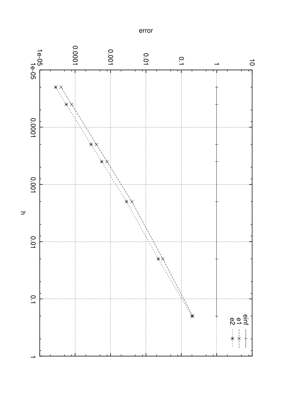
Let us define two discrete function norms to measure the convergence:
| (5) |
We can compute that
| (6) |
and therefore there is no convergence in infinite norm for . In and , we can respectively observe the convergence with order on Figure 2(d).
Complementarity framework
Let us end this section by restating the systems (1) and (2) into the complementarity framework. Let us introduce equivalent formulations of the inclusion such that
| (7) |
where is the normal cone in the sense of Convex Analysis to the interval . The definition of the normal cone in the present case,
| (8) |
yields the following complementarity representation of the sign multi-valued function
| (9) |
In order to directly substitute the value of into the dynamics , a other complementarity formulation can be defined. By setting and , one gets
| (10) |
3 A class of differential inclusions
Let us now introduce the following class of differential inclusions, where :
| (11) |
The following assumption is made:
Assumption 1
The following hold:
- •
(i) is a multivalued maximal monotone operator from into , with domain , i.e., for all and all , one has
(12) - •
(ii) There exists such that for all , for all , one has .
- •
(iii) There exists a function such that for all :
.
Proposition 1
In this paper we shall focus on inclusions of the form:
| (13) |
Example 1 (Equivalent-control-based sliding-mode-control (ECB-SMC))
Let us now state a well-posedness result which is a consequence of Proposition 1.
Corollary 1
Proof: The proof uses a state variable change introduced in [13]. Let be the symmetric square root of , i.e. . Let us perform the state transformation . Then we get
| (15) |
Notice that . Therefore . We can rewrite the system as
| (16) |
The multivalued mapping is monotone. By [46, Exercise 12.4] it follows that each multivalued mapping is monotone. From [29, Proposition 1.3.11] it follows that with . By [45, Theorem 5.7] it follows that is convex. Being the subdifferential of a convex function, the multivalued mapping is maximal (monotone) [45, Corollary 31.5.2]. Therefore by Proposition 1 the inclusion in (16) possesses a unique Lipschitz solution on for any and since is full–rank so does (13).
Example 2
Example 3
Consider , . Trajectories may slide on codimension one surfaces or and on the codimension 2 surface ( and ).
Example 4
One solution to reduce chattering is the observer based SMC. Let us consider the following example taken from [55], whose closed-loop dynamics is given by:
Notice that the condition (14) implies that . When this is a relative degree one condition. It is noteworthy that (14) does not imply that has full column rank. In particular it does not preclude . Dissipative systems with no feedthrough matrix satisfy an input-output constraint similar to (14) [14].
Example 5 (Lyapunov-based discontinuous robust control)
Let us show how the above material adapts to this type of feedback controller. The class of dynamical systems is
| (18) |
where , , satisfies assumption 1, and is a bounded disturbance satisfying for all , all and some finite . The problem is the stabilization of the system at the origin , knowing that there exists a function such that the uncontrolled undisturbed system admits as a Lyapunov function. In particular, one has along the trajectories of the free system. Let us rewrite the system in (18) as
| (19) |
Let us propose the control input . We obtain:
| (20) |
We can state the following result.
Corollary 2
Suppose that , . The system in (20) has a unique Lipschitz continuous solution on for any .
Proof: We have . Let , where is the symmetric square root of . We may rewrite (20) as
Then following the same steps as for the proof of Corollary 1 we conclude that Proposition 1 applies to this system, hence to (20).
Such a controller assures the global asymptotic stability of the equilibrium . This is made possible because of the multivalued characteristic of the discontinuous input. The closed-loop system possesses the origin as its unique equilibrium, because of the multivaluedness property. The restriction to quadratic Lyapunov functions stems from monotonicity preserving conditions, and is not straightforwardly avoided.
4 Convergence results and Chattering Free Finite–time Stabilization
The differential inclusion (11) is time-discretized on with a backward Euler scheme as follows:
| (21) |
where . The fully implicit method uses instead of . The convergence and order results stated in Proposition 2 below have been derived for the semi-implicit scheme (21) in [10]. So the analysis in this section is based on such a discretization. However this is only a particular case of a more general method which is used in practical implementations. The next result is proved in [10].
Thus the numerical scheme in (21) has at least order , and convergence holds. The conditions of Assumption 1 for the existence and uniqueness results of Proposition 1 are sufficient only. Other criteria exist, like Filippov’s criterion for uniqueness of solutions [18, Proposition 5]. Similarly it is possible that time-stepping methods converge for systems that satisfy such a criterion, despite no result seems to be available in the literature. As seen in Lemma 1, the precision of the method may be much better than what is to be expected from (22) on large portions of the trajectories.
The differential inclusion in (13) is therefore discretized as follows:
| (23) |
One sees that advancing the implicit method from step to step involves solving generalized equations with unknown , of the form where is singlevalued while is multivalued. , and appear as parameters of the generalized equations. Solving such generalized equations thus boils down to computing the intersection between the graph of and the graph of as illustrated in section 2. The result of Proposition 2 applies to (23). As we shall see next, such an implicit method also assures a good estimate of the derivative and a smooth stabilization of the discrete-time solution on the sliding surface.
Before stating the smooth stabilization result, let us consider a preliminary result. Let us denote the output of the dynamical as:
| (24) |
Lemma 2
Let us assume that a sliding mode exists for some indices such that
| (25) |
Then there exists such that for all and for all such that , one has
| (26) |
Furthermore, let Assumption 1.(ii) holds, then the following bound is satisfied in the neighborhood of the sliding subspace,
| (27) |
for all such that .
Proof: From (25), we have . For , the sliding mode implies that for all and therefore
| (28) |
The inclusion (28) yields
| (29) |
for all such that . By the assumption 1.(ii), the Lipschitz continuity of allows us to write for some
| (30) |
Lemma 3
Let us assume that a sliding mode occurs for the index , that is . Let and be such that (14) holds and . Then there exists such that , there exists such that for all integers .
Proof: At each time–step, we have to solve for and the generalized equation
| (31) |
Under condition (14), the convergence of the time–stepping scheme is ensured by Proposition 2. The convergence and the existence of the sliding mode ensure that
| (32) |
for . Using (27) for and a sufficiently small such that , we have the following bound
| (33) |
Introducing the complementary index set , for almost everywhere and using (33) we obtain that there exists such that
| (34) |
and therefore it is possible to choose such that for all
| (35) |
If (35) is satisfied, the unique solution of (31) at the iteration is given by
| (36) |
The next iterate will by given by the solution of the generalized equation,
| (37) |
Using the fact that , we can use (29) to conclude that there exists such that for all
| (38) |
and therefore the solution of (37) is
| (39) |
The bound (29) is uniform and can be applied for the next steps. Choosing as the minimum of the considered time steps , the proof is obtained for .
The finite-time convergence of the time-discretization of similar nonsmooth dynamical systems (essentially mechanical systems with dry friction) is proved in [6]. Our results may therefore be considered as the continuation of studies on the finite-time convergence for algorithms of the proximal type.
5 Discrete–time Sliding Mode Control (SMC)
This section is devoted to show how the above discretizations may be used in a digital control framework.
5.1 Example of an implicit Euler controller (IEC)
Let us come back to the inclusion in (1). For this simple system, the ZOH and the Euler discretization yield the same–discrete system. Assume the integrator is sampled with sampling period . On the time interval one has , where . The controller is known as the equivalent control-based SMC [57]. Let us implement a “backward” controller at time , following the above lines. Suppose that . Then following the same calculations as in the proof of Lemma 1, we obtain that . Therefore on :
| (40) |
and it follows that . On the next sampling interval one obtains
| (41) |
and so on on the next intervals, where the zero value is obviously some small value at the machine accuracy. if we suppose that , the value of is or according to the sign of . To summarize the control is given explicitly in terms of and by
| (42) |
where denotes the Euclidean projection operator onto the set .
As alluded to above, such an “implicit” input is causal and can be computed at with the values of the state at by (42). It requires at each step to solve a rather simple multivalued problem which a Mixed Linear Complementarity Problem (MLCP, see Section 6 below). It is not of the high gain type.
Remark 1
The fact that the function sgn generates only binary values ( or ) does not hamper the above method to work. Indeed the implicit Euler method allows us to compute values of the sign multifunction inside its multivalued part at .
5.2 Extension to ZOH discretized systems
The ZOH discretization of linear time invariant systems with an ECB-SMC controller, results in a discrete-time system of the form:
| (43) |
where is the sampling period, and
| (44) | |||||
| (45) |
with , , when a explicit Euler implementation of the control is performed [52, 56]. For an implicit Euler implementation, let us set
| (46) |
which corresponds to the implicit discrete time version of the ECB-SMC controller. We therefore get on each sampling period:
| (47) |
At each time–step, one has to solve
| (48) |
Inserting the first line of (48) into the second line we obtain the following one–step system
| (49) |
Comparing with the time–discretized systems in (23) and (31) one sees that the term is replaced in case of a ZOH method by the term . Provided the problem has a unique solution one can compute the controller in (46) with the knowledge of , , , and . We will see in the next Section how the computation can be carried out in practice.
6 Implementation of Discrete–Time Systems
Let us consider in this section the following discrete–time system:
| (50) |
where is an integer, the discrete state, the discrete output and the discrete input. The discrete system (50) is a common representative for the discretization given by (23), (21) or (48) and the matrices , and the vector are determined by the chosen time–discretization method and detailed in Section 6.2. The matrices and are given by their definition in (13).
6.1 Mixed Linear Complementarity Problem (MLCP)
The time–discretized system (50) appears to be a Mixed Linear Complementarity Problem (MLCP) that we have to solve at each time–step. Let us define what is a MLCP in its general form with bounds constraints as it has been proposed in [21]:
Definition 1 (MLCP)
Given a matrix , a vector and lower and upper bounds , find , such that
| (51) |
where .
Note that the problem (51) implies that
| (52) |
where the notation is used for the normal cone in the Convex Analysis sense to a convex set at the point . The box is defined by the Cartesian product of the intervals . The normal cone to a convex set is a standard instance of a multi–valued mapping [45]. The relation (52) is equivalent to the MCP (51) if we assume that is the positive part of , that is and is the negative part of , that is .
In order to state the problem (50) as a MLCP, the variable is condensed into the second line such that
| (53) |
and the following variable and parameters are defined as follows
| (54) |
Finally, the problem (50) can be recast into a MLCP by observing that
| (55) |
The MLCP (51) is a well-known problem in the mathematical programming theory arising for instance from the Karush–Kuhn–Tucker optimality conditions of a quadratic program or from the primal/dual optimality conditions of a linear program. The MCLP enjoys a large number of numerical algorithms and several reliable solvers have been implemented. Several families of solvers may be cited: a) extensions of Lemke and principal pivotal techniques for LCP to MLCP [48, 47, 21, 17] b) extensions of projection/splitting techniques for MLCP [24, 19] and c) semi–smooth Newton methods [40]. In this paper, the computations are done with the help the Siconos/Numerics open source Library [3] and/or the PATH solver [21]. The results of existence and uniqueness of solutions of (51) are related to the properties of (P-properties or coherent orientations of the associated affine map (normal map) for particular cases of bounds constraints). Without entering into further details, we refer to [30, 24] for the main results. The assumptions on the matrix drives the choice of particular solvers that can be in polynomial time rather than standard exponential time for brute force enumerative solvers.
6.2 Some Time–Discretization Methods
In this Section, the formulation of the discrete–time system (50) is related to the continuous time system (13) through a given discretization method.
Explicit Euler discretization of
Let us start with the explicit Euler discretization method of the term as it has been given in (21). At each time step, the matrices in (50) and in the MLCP (51) can be identified as
| (56) |
Let the assumptions of Corollary 1 be satisfied with full–column rank (). This result ensures the existence and uniqueness of a solution of the MCLP. Furthermore, standard pivotal techniques such as Lemke’s method or projection/splitting such as Projected Successive Over-Relation (PSOR) compute the solution.
Implicit Euler and - method
In a more general way, we can choose to time–discretize the term by a implicit Euler scheme or a -method. The main motivation for doing in this way is the higher accuracy and stability that we can obtain for such a numerical integration scheme (see [2] for an example of instability with the Explicit Euler method). Let us consider first that the mapping is affine, that is . The matrices in (50) and in the MLCP (51) can be identified as
| (57) |
for . For , the explicit Euler case is retrieved. For , the implicit Euler scheme is used to discretize . If the mapping is nonlinear, a newton linearization can be invoked. In this case, the solution at each time step is sought as a limit of solutions of successive MLCPs. We refer to [2] for a detailed presentation of these developments.
Zero–Order Holder (ZOH) method
The ZOH discretization presented in Section 5.2 can be also formalized into the form (50) and then (51) with
| (58) |
In practice, numerous methods are available to compute the ZOH discretization, i.e., and which amounts to compute the matrix exponential and its time integral [39]. In this work, the numerical computation is performed using an explicit Runge–Kutta method with high order of accuracy and a numerical tolerance near the machine precision threshold. On the Figure 3, the control scheme is depicted showing that the controller is causal and computed form .
7 Two other classes of differential inclusions
In this section, we introduce other classes of differential inclusions which extend (13). The second class of differential inclusions is:
| (59) |
with , , , is a scalar.
The third class that we shall analyze is:
| (60) |
where and are smooth functions, .
Corollary 3
The proof is straightforward and is omitted.
Example 6
The mapping , is hypomonotone. Indeed and is monotone for any .
Example 7
Let , be reals. The mapping , , is hypomonotone with constant for any . Let . Then . The linearized Stribeck friction model (with multivalued part at zero tangential velocity) [38] is hypomonotone.
Lemma 4
Let for some , and Ker Ker. Then for any initial data the differential inclusion (59) has a unique solution that is Lipschitz continuous..
Proof: First notice that the set-valued mapping is maximal monotone [46, Exercise 12.4]. Under the lemma’s conditions, one sees that is continuous on the surface . Indeed the jump of the vector field is equal to on . Moreover it is Lipschitz continuous as it is piececewise linear. Hence Proposition 1 applies.
Corollary 4
The proof is straightforward and is omitted.
Example 8
The mapping , , is hypomonotone with any .
Remark 2
As noted in [55] chattering may be due in sliding mode control appplications to the presence of parasitic dynamics. Simple modelling of these yield when inserted in (1) the differential inclusion (see [55, (7) (8)])
| (61) |
with . The relative degree of the triplet of this system is , where and . This system does not fit within the above classes of inclusions. Similar conclusions hold for the other form of parasitics in [55, (3) (4)]. Such parasitics may be seen as a non collocation issue, that is known to greatly influence the stability of systems and usually may yield instability. The mere existence and uniqueness of solutions for such relative degree 3 systems is not trivial. In [42] an example is given that possesses an infinity of absolutely continuous Filippov’s solutions, but a unique so-called forward solution. One interesting question is to determine what kind of solution is approximated by the backward Euler method applied to (61) which, according to [42, Theorem 1] has a unique forward solution since its leading Markov parameter is . A possible solution for this non collocation issue is the observer design of Example 4.
The differential inclusions in (59)–(60) are therefore discretized as follows:
| (62) |
and
| (63) |
where the are the hypomonotonicity constants and . The result of Proposition 2 applies to (62) and (63).
7.1 A simple hypomonotone case
As shown in Section 2 on a simple monotone example, in practice the intersection may be computed as follows. Let us now illustrate this on the following system with hypomonotone multivalued part:
| (64) |
with . We may discretize it as:
| (65) |
Notice that we may rewrite (65) as
| (66) |
Let us denote the mapping in the right-hand-side of (66) as . The set-valued mapping is strongly monotone [24, Definition 2.3.1] for all . It follows from [24, Theorem 2.3.3] that the generalized equation has a unique solution.
For , the following Lemma extends the Lemma 1.
Lemma 5
For all and , there exists such that and for all .
Proof:If , then . Otherwise, for and , the solution is given by :
| (67) |
From the solution (67), the step for which can be easily found. Let us now consider that . The only possible solution for
| (68) |
is and . For the next iteration, we have to solve
| (69) |
and we obtain and . The same holds for all ,, , redoing the same reasoning. Clearly then the terms approximating the derivative, are zero for any .
We conclude that in this case also the system and its derivative are correctly approximated at the zero value on the sliding surface. There is no spurious oscillation around the switching surface.
8 Detailed Implementation of Implicit Euler Discretization of the general case (60)
This section is devoted to the implementation and the study of the numerical algorithm. The interval of integration is , , and a grid , , , is constructed. The approximation of a function on is denoted as , and is a piecewise constant function, constant on the intervals . We denote as . The time-step is .
8.1 Time–discretization
Starting from (60), let us introduce a new notation,
| (70) |
where and are complementary variables related through the multi–valued mapping. According to the class of systems (13), (59) or (60) that we are studying the functions and are defined either in a fully nonlinear framework or by affine functions. We present the time-discretization in its full generality and specialize the algorithms for each case in Section 8.4.
Let us now proceed with the time discretization of (70) by a fully implicit scheme :
| (71) |
where , , and , with and . As in [1], we call the problem (71) the “one–step nonsmooth problem”.
This time-discretization is slightly more general than a standard implicit Euler scheme. The main discrepancy lies in the choice of a -method to integrate the nonlinear term. For , we retrieve the explicit integration of the smooth and single valued term . Moreover for , the term is explicitly evaluated. The flexibility in the choice of and allows the user to improve and control the accuracy, the stability and the numerical damping of the proposed method. For instance, if the smooth dynamics given by is stiff, or if we have to use large step sizes for practical reasons, the choice of offers better stability properties with respect to .
8.2 Mixed Complementarity Problem
The so-called "one–step nonsmooth problem” (71) appears to be a Mixed Complementarity Problem (MCP) that we have to solve at each time–step. Let us define what is a MCP :
Definition 2 (MCP)
Given a function and lower and upper bounds , find , such that
| (72) |
where .
Note that the problem (72) implies that
| (73) |
The relation (73) is equivalent to the MCP (72) if we assume that is the positive part of , that is and is the negative part of , that is .
The One–step nonsmooth problem as a MCP
Let us define the MCP by
| (74) |
If solves the MCP (74), the bounds and and the condition imply that
| (75) |
The MCP is then given by
| (76) |
It is clear that the problem (71) is equivalent to the MCP defined by (74). The results of existence and uniqueness of solution of (72) or equivalently (73) are related to the monotonicity properties of (P-properties or coherent orientations of the associated affine map for particular cases of bounds and affine function . Without entering into further details, we refer to [30, 24] for the main results.
Numerical Solvers
The MCP (72) can be solved by a large family of solvers based on Newton–type Methods and interior-points techniques. We refer to [11] for a comparison of several solvers based on Newton’s method. The numerical implementation of the MCP solvers are often based on the computation of the Jacobian matrix of the function with respect to . The Jacobian matrix is explicitly given in the case defined in (74) by
| (77) |
where denotes the simple contracted tensor product and the third–order tensor is the Jacobian of with the respect given by the following component:
| (78) |
8.3 Newton’s linearization and Mixed Linear Complementarity Problems
Due to the fact that two of the systems that are studied in this paper involve affine functions and , we propose to solve the "one–step nonsmooth problem” (71) by performing an external Newton linearization, which yields a Mixed Linear Complementarity Problems (MLCP).
Newton’s linearization
The first line of the problem (71) can be written under the form of a residue depending only on and such that
| (79) |
with . The solution of this system of nonlinear equations is sought as a limit of the sequence such that
| (80) |
The computation of the Jacobian of with respect to , denoted by leads to
| (81) |
At each time–step, we have to solve the following linearized problem,
| (82) |
that is
| (83) |
The matrix is clearly non singular for small . The same operation is performed with the second equation of (71) leading to the following linearized equation
| (84) |
Inserting (83), we get the following linear relation between and ,
| (85) |
Mixed linear complementarity problem (MLCP)
To summarize, the problem to be solved in each Newton iteration is:
(86)
with and defined by
| (87) |
The problem (86) is equivalent to a MLCP which can be solved under suitable assumptions by many linear complementarity solvers such as pivoting techniques, interior point techniques and splitting/projection strategies. The reformulation into a standard MLCP follows the same line as for the MCP in the previous section. One obtains,
| (88) |
As for the MCP, there exists numerous methods to numerically solve MLCP. In the worst case when the matrix has no special properties, the MCLP can be always solved by enumerative solvers for which various implementations can be found. With some positiveness properties [24], standard methods for LCP[19] can be straightforwardly extended. Among these methods, we can cite the family of projection/splitting methods, interior point methods and semi-smooth Newton methods (see [1] for an overview).
8.4 The special cases of the affine systems
In this section, we specify the time–discretization to the two other classes of systems (13) and (59) and for particular value of and .
8.4.1 Time–discretization of the system (13)
For the system (13), the function is reduced to the matrix and the function is affine, that is . The matrix and are then given by
| (89) |
with
| (90) |
If then the matrix is also positive definite for sufficiently small . This result ensures the existence and uniqueness of a solution of the MCLP. Furthermore, standard pivoting techniques such as Lemke’s method or projection/splitting such as Projected Successive Over-Relation (PSOR) compute the solution.
Semi-implicit discretization with
The matrix is then reduced to
| (91) |
and
| (92) |
In this particular case, there is no need to perform some Newton iterations because the system to be solved at each time–step is linear. Furthermore, the MLCP has a solution for any under the assumptions that .
Fully implicit discretization with an affine function
The same conclusion can be drawn if is equal to a constant matrix that is when is linear time-invariant and given by . In this case, the matrix reduces to
| (93) |
and
| (94) |
8.4.2 Time–discretization of the system (59)
For the system (59), we recall that and are given by
| (95) |
The components of can be explicitly expressed by
| (96) |
and therefore, the Jacobian of is given by
| (97) |
The Jacobian of takes the following simple form:
| (98) |
After the newton linearization, we have to solve at each Newton’s loop the MLCP (86) with
| (99) |
Semi–implicit discretization with
If and vanish, the residue given by
| (100) |
is linear in and . In this particular case, there is no need to perform Newton’s iterations. The MCLP defined by (99) can be simplified to
| (101) |
8.5 Algorithms
We propose in this section two algorithms to sum-up the numerical implementation of the implicit Euler time–stepping scheme. The Algorithm 1 describes the implementation with a generic MCP solver and the Algorithm 2 describes the numerical implementation of the algorithm with an external Newton linearization and a MCLP solver.
9 Numerical experiments
Let us illustrate the above developments with numerical integrations performed with the siconos software platform of the INRIA22 2 http://siconos.gforge.inria.fr/ [1, 3] which is designed for the simulation of multivalued nonsmooth systems.
9.1 Chattering free stabilization
Let us consider the following continuous–time closed loop system from [26] given by
| (102) |
As it is shown in [26] the trajectories obtained by an explicit Euler discretization exhibit spurious oscillations which are described by period-2 cycle around the sliding manifold. On Figure 4, the trajectories obtained by implicit discretization are shown using the implicit Euler discretization with , , and and with and . As it has been predicted by theoretical discussions of Section 4, the sliding manifold is reached in finite time and without any chattering. Indeed, the matrix satisfies the assumptions of Lemma 3. Note that the algorithm is also very robust in the sense that the simulation can be performed with relatively large time–steps.


9.2 Example 3: Multiple sliding surfaces


9.3 Extensions to ZOH discretized systems
The extension to ZOH discretized systems is illustrated on a first example taken from [27]. In the notation of Section 5.2, the LTI system with an ECB-SMC controller is defined by the following data,
| (104) |
Starting from the initial data, , Galias and Yu [27] have shown that the Explicit ZOH discretization of the system with , , and exhibits a period–2 orbit. The results are reproduced on Figure 6(a). On Figure 6(b), the Implicit ZOH discretization as proposed in Section 5.2 is free of chattering. On Figure 7, a comparison is given between the ZOH and the Euler discretization of the vector field .


Another example taken from [57] in the MIMO case is given by the following parameters,
| (105) |
Similar results are depicted on Figure 8.


9.4 Lyapunov-based robust control
We propose in this section to give an numerical example which fits with the example (18) of a Lyapunov-based discontinuous robust control. Let us consider the following system
| (106) |
with and . Is is obvious that, as expected, the implicit method yields a smooth stabilization at whereas the explicit Euler has significant chattering. Figure 9(c) illustrates the fact that the controller varies inside the multivalued part of the sgn function in order to assure the existence of an equilibrium point.


9.5 The Filippov example
Example 9
Let us consider now the well known Filippov example which can be defined in the form (13) with
| (107) |
The trajectories may slide on the codimension 2 surface given by , that .


9.6 Example 4: Observer based SMC
Let us illustrate the performance of our implementation on the observer based SMC described by the Example 4. The dynamics is given by (17) with and . The initial conditions are chosen as . The numerical parameters are given by that is a sampling of and . On Figure 11, the error between the reference command and the observer state is given. On Figure 12, we can observe the behavior of the command without any chattering.


On the three previous examples, one sees a very accurate and smooth stabilization on the sliding surface, even for values of not so small.
Influence of the integration parameters and
In the following numerical experiments, we discuss the role of the numerical parameters and . Due to the fact that the function is linear and reduced to a matrix , the parameter has no influence on the numerical time–integration. On the contrary, the parameter has a huge influence on the stability of the integration. Indeed, the implicit Euler integration ( of the smooth term is unconditionally stable. This is not the case for the explicit Euler and for the chosen parameters and , the instability of the scheme for does not allow to proceed to integration. On Figure 13, the instability of the scheme is illustrated and appears as a chattering on the state . The stability is retrieved for .

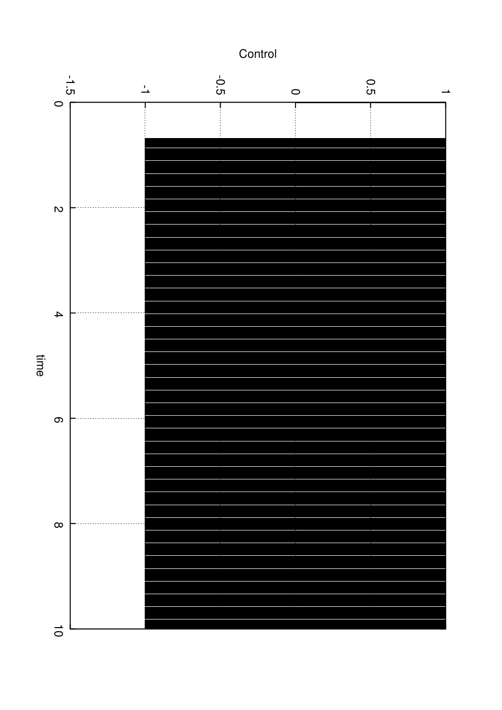
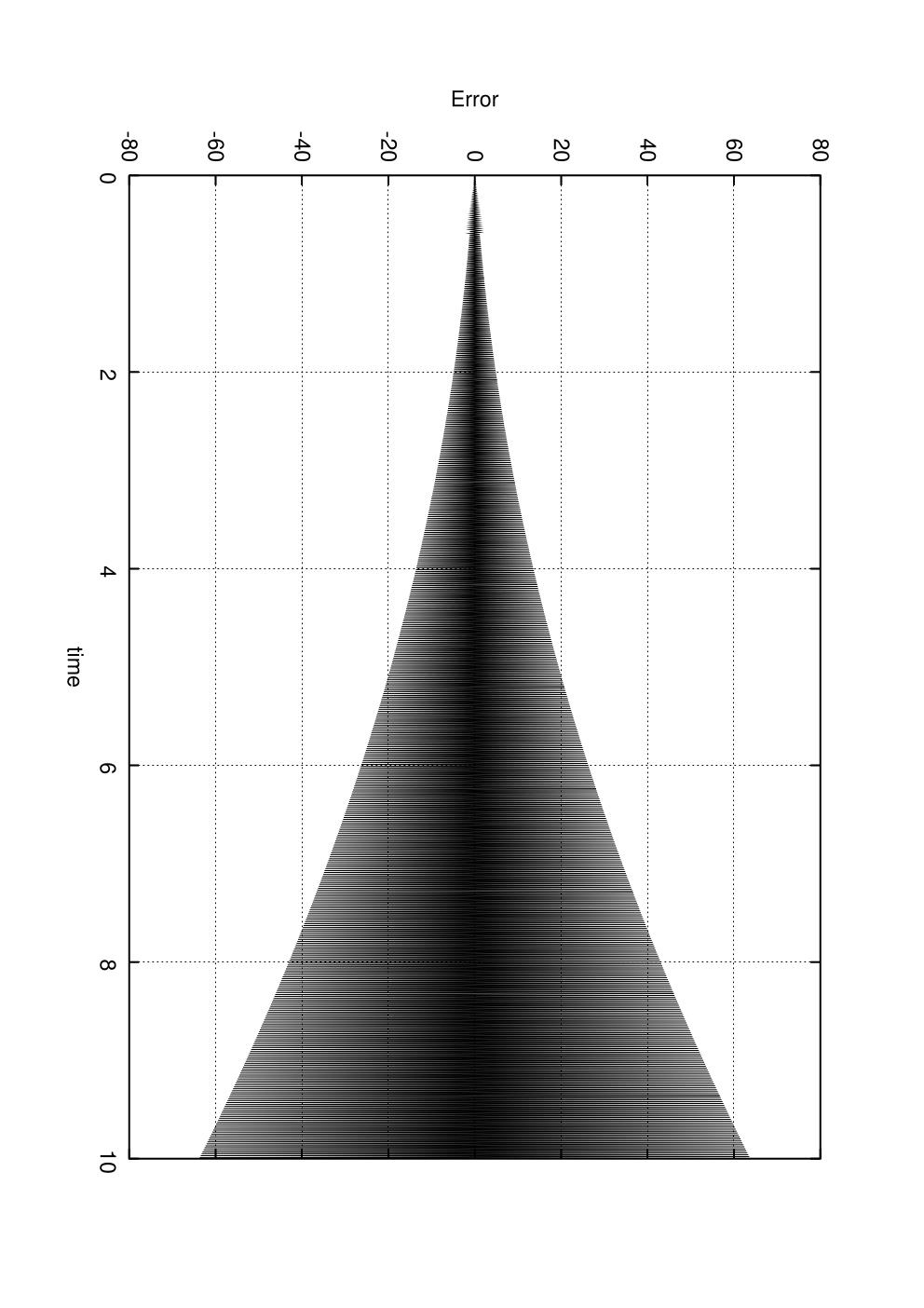
Other choices of can be made to improve the numerical time–integration of the smooth dynamics. For instance, yields a second order scheme for the integration of . Unfortunately, the scheme is not of second order due to the fully implicit integration of the multi-valued part. Nevertheless, it can be interested to use of to decrease the numerical damping of the scheme on the smooth term. On the Figure 14, two simulations of the observer based SMC are presented for and . The parameter has been modified to to correctly integrate the parasitic dynamics with the same time–step .


10 Conclusions
In this paper the backward Euler method is studied on specific classes of Filippov’s systems that encompass sliding mode control systems. It is shown that such implict schemes allow a smooth accurate stabilization on the sliding surface, even in case of codimension larger than one. Despite the backward Euler method has been studied and used for a long time in other fields like contact mechanics and electric circuits simulation [1], it seems it has not yet been used in the sliding mode control community. This work therefore constitutes the introduction of a new discretization method for EBC-SMC systems. The novelty compared to numerical simulation is that this time one has to consider not only the numerical simulation, but also the implementation on real processes. Perhaps one obstacle to the dissemination of the method is that at first sight, the controller designed from a backward philosophy looks like a non causal controller. However as shown in this paper this is not the case. This paper paves the way towards the study of a new family of discrete-time sliding mode controllers.
References
- [1] V. Acary and B. Brogliato. Numerical Methods for Nonsmooth Dynamical Systems: Applications in Mechanics and Electronics, volume 35 of Lecture Notes in Applied and Computational Mechanics. Springer Verlag, 2008.
- [2] V. Acary and B. Brogliato. Implicit Euler numerical simulation of sliding mode systems. Technical Report RR 1234567890, INRIA, 2009.
- [3] V. Acary and F. Pérignon. An introduction to siconos. Technical Report TR-0340, INRIA, http://hal.inria.fr/inria-00162911/en/, 2007.
- [4] J.C. Alexander and T.I. Seidman. Sliding modes in intersecting switching surfaces. I: Blending. Houston J. Math., 24(3):545–569, 1998.
- [5] J.C. Alexander and T.I. Seidman. Sliding modes in intersecting switching surfaces. II: Hysteresis. Houston J. Math., 25(1):185–211, 1999.
- [6] B. Baji and A. Cabot. An inertial proximal algorithm with dry friction: finite convergence results. Set-Valued Anal., 14(1):1–23, 2006.
- [7] O. Barambones, P. Alkorta, A.J. Garrido, I. Garrido, and F.J. Maseda. An adaptive sliding mode control scheme for induction motor drives. Int. J. Circuits, Systems and Signal Processing, 1(1):73–78, 2007.
- [8] G. Bartolini, L. Fridman, A. Pisano, and E. Usai, editors. Modern Sliding Mode Control Theory. New Perspectives and Applications, volume 375 of LNCIS. Springer Verlag, 2008.
- [9] J. Bastien and C.H. Lamarque. Persoz’ gephyroidal model described by a maximal monotone differential inclusion. Arch. Appl. Mech., 78(5), 2008.
- [10] J. Bastien and M. Schatzman. Numerical precision for differential incusions with uniqueness. ESAIM M2AN: Mathematical Modelling and Numerical Analysis, 36(3):427–460, 2002.
- [11] S.C. Billups, S.P. Dirkse, and M.C. Ferris. A comparison of large scale mixed complementarity problem solvers. Computational Optimization and Applications, 7:3–25, 1997.
- [12] I. Boiko, L. Fridman, A. Pisano, and E. Usai. A comprehensive analysis of chattering in second order sliding mode control systems. Bartolini, Giorgio (ed.) et al., Modern sliding mode control theory. New perspectives and applications. Berlin: Springer. Lecture Notes in Control and Information Sciences 375, 23-49 (2008)., 2008.
- [13] B. Brogliato. Absolute stability and the Lagrange-Dirichlet theorem with monotone multivalued mappings. Systems and Control Letters, 51:343–353, 2004.
- [14] B. Brogliato, R. Lozano, B. Maschke, and O. Egeland. Dissipative Systems Analysis and Control. Theory and Applications. Springer Verlag, London, 2nd edition, 2007.
- [15] B. Brogliato and A. Trofino Neto. Practical stabilization of a class of nonlinear systems with partially known uncertainties. Automatica, 31(1):145–150, 1995.
- [16] M. K. Camlibel, W.P.M.H. Heemels, and J.M. Schumacher. Consistency of a time-stepping method for a class of piecewise-linear networks. IEEE Trans. Circuits and systems I, 49:349–357, 2002.
- [17] M. Cao and M.C. Ferris. A pivotal method for affine variational inequalities. Mathematics of Operations research, 21(1):44–64, 1996.
- [18] J. Cortes. Discontinuous dynamical systems. a tutorial on solutions, nonsmooth analysis, and stability. IEEE Control Systems Magazine, pages 36–73, June 2008.
- [19] R. W. Cottle, J. Pang, and R. E. Stone. The Linear Complementarity Problem. Academic Press, Inc., Boston, MA, 1992.
- [20] M.-F. Danca. Numerical approximations of a class of switch dynamical systems. Chaos Solitons Fractals, 38(1):184–191, 2008.
- [21] S. P. Dirkse and M. C. Ferris. The PATH solver: A non-monotone stabilization scheme for mixed complementarity problems. Optimization Methods and Software, 5:123–156, 1995.
- [22] A.L. Dontchev and F. Lempio. Difference methods for differential inclusions: a survey. SIAM reviews, 34(2):263–294, 1992.
- [23] C. Edwards, E. Fossas Colet, and L. Fridman, editors. Advances in Variable Structure and Sliding Mode Control, volume 334 of LNCIS. Springer Verlag, 2006.
- [24] F. Facchinei and J. S. Pang. Finite-dimensional Variational Inequalities and Complementarity Problems, volume I & II of Springer Series in Operations Research. Springer Verlag NY. Inc., 2003.
- [25] Z. Galias and X. Yu. Complex discretization behaviors of a simple sliding-mode control system. IEEE Transactions on Circuits and Systems – II: Express Briefs, 53(8):652–656, August 2006.
- [26] Z. Galias and X. Yu. Euler’s discretization of single input sliding-mode control systems. IEEE Transactions on Automatic Control, 52(9), September 2007.
- [27] Z. Galias and X. Yu. Analysis of zero–order holder discretiation of two–dimensional sliding–mode control systems. IEEE Transactions on Circuits and Systems – II: Express Briefs, 55(12), December 2008.
- [28] W. Garcia-Gabin, D. Zambrano, and E.F. Camacho. Sliding mode predictive control of a solar air conditioning plant. Control Engineering Practice, 2009. in press.
- [29] D. Goeleven, D. Motreanu, Y. Dumont, and M. Rochdi. Variational and Hemivariational Inequalities: Theory, Methods and Applications; Volume I: Unilateral Analysis and Unilateral Mechanics. Nonconvex Optimization and its Applications. Kluwer Academic Publishers, 2003.
- [30] P.T. Harker and J.-S. Pang. Finite-dimensional variational inequality and complementarity problems: a survey of theory, algorithms and applications. Mathematical Programming, 48:160–220, 1990.
- [31] G. Herrmann, S.S. Ge, and G. Guo. Practical implementation of a neural network controller in a hard disk drive. IEEE Transactions on Control Systems Technology, 13(1):146–154, January 2005.
- [32] R.A. Hess and S.R. Wells. Sliding mode control applied to reconfigurable flight control design. J. of Guidance, Control, and Dynamics, 26(3):452–462, May–June 2003.
- [33] Q. Hu, C. Du, L. Xie, and Y. Wang. Discrete-time sliding mode control with time-varying surface for hard disk drives. IEEE Transactions on Control Systems Technology, 17(1):175–183, January 2009.
- [34] A.E. Kastner-Maresch. The implicit midpoint rule applied to discontinuous differential equations. Computing, 49:45–62, 1992.
- [35] A. Koren and M. Idan. Integrated sliding mode guidance and control for a missile with on-off actuators. J. of Guidance, Control, and Dynamics, 31(1):204–214, January–February 2008.
- [36] A.J. Koshkouei and A.S.I. Zinober. Sliding mode control of discrete-time systems. Journal of Dynamic Systems, Measurement, and Control, 122:793–802, December 2000.
- [37] R. Leine and H. Nijmeijer. Dynamics and Bifurcations of Non-Smooth Mechanical Systems. Springer Verlag, Lecture Notes in Applied and Computational Mechanics 18, 2004.
- [38] L. Marton and B. Lantos. Control of mechanical systems with stribeck friction and backlash. Systems and Control Letters, in press. doi:10.1016/jsysconle.2008.10.001.
- [39] C. Moler and C. Van Loan. Nineteen dubious ways to compute the exponential of a matrix, twenty-five years later. SIAM Rev., 45(1):3–49, 2003.
- [40] T. S. Munson, F. Facchinei, M. C. Ferris, A. Fischer, and C. Kanzow. The semismooth algorithm for large scale complementarity problems. INFORMS Journal on Computing, 13:294–311, 2001.
- [41] Y. V. Orlov. Discontinuous Systems. Lyapunov Analysis and Robust Synthesis under Uncertainty Conditions. Communications and Control Engineering. Springer verlag, London, 2009.
- [42] A. Y. Pogromski, W.P.M.H. Heemels, and H. Nijmeijer. On solution concepts and well-posedness of linear relay systems. Automatica, 39:2139–2147, 2003.
- [43] A.B. Proca, A. Keyhani, and J.M. Miller. Sensorless sliding-mode control of induction motors using operating condition dependent models. IEEE Transactions on Energy Conversion, 18(2):205–212, June 2003.
- [44] E. Promtun and S. Seshagiri. Sliding mode control of a pitch-rate of an f-16 aircraft. Int. J. of Applied Science, Eng. and Technology, 5(1):1–7, 2009.
- [45] R.T. Rockafellar. Convex Analysis. Princeton University Press, 1970.
- [46] R.T. Rockafellar and R.J.-B. Wets. Variational Analysis, volume 317. Springer Verlag, New York, 1997.
- [47] T. Rutherford. Miles: A mixed inequality and nonlinear equation solver, 1993.
- [48] R. W. H. Sargent. An efficient implementation of the Lemke algorithm and its extension to deal with upper and lower bounds. Mathematical Programming Study, 7:36–54, 1978.
- [49] D. Stewart. A high accuracy method for solving ODEs with discontinuous rigth–hand–side. Numerische Mathematik, 58:299–328, 1990.
- [50] D. Stewart. A numerical method for friction problems with multiple contacts. J. Austral. Math. Soc. Ser. B, 37:288–308, 1996.
- [51] Y.C. Tsai and A.C. Huang. Multiple-surface sliding controller design for pneumatic servo systems. Mechatronics, 18(9):506–512, November 2008.
- [52] B. Wang, X. Yu, and G. Chen. ZOH discretization effect on single-input sliding mode control systems with matched uncertainties. Automatica, 45:118–125, 2009.
- [53] W.J. Wang and J.Y. Chen. Passivity-based sliding mode position control for induction motor drives. IEEE Transactions on Energy Conversion, 20(2):316–321, June 2005.
- [54] S.R. Wells and R.A. Hess. Multi-input/multi-output sliding mode control for a tailles fighter aircraft. J. of Guidance, Control, and Dynamics, 26(3):463–473, May–June 2003.
- [55] K.D. Young, V.I. Utkin, and U. Ozguner. A control engineer’s guide to sliding mode control. IEEE Transactions on Control Systems Technology, 7(3):328–342, May 1999.
- [56] X. Yu and G. Chen. Discretization behaviors of equivalent control based sliding-mode control systems. IEEE Transactions on Automatic Control, 48(9):1641–1646, September 2003.
- [57] X. Yu, B. Wang, Z. Galias, and G. Chen. Discretization effect on equivalent control-based multi-input sliding-mode control systems. IEEE Transactions on Automatic Control, 53(6):1563–1569, July 2008.