We study the two component $\phi^{4}$ model on a simple cubic lattice. We label the sites of the lattice by $x=(x_{0},x_{1},x_{2})$. The components of $x$ might assume the values $x_{i}\in\{1,2,...,L_{i}\}$. We simulate lattices of the size $L_{1}=L_{2}=L$ and $L_{0}\ll L$. In 1 and 2-direction we employ periodic boundary conditions and free boundary conditions in 0-direction. This means that the sites with $x_{0}=1$ and $x_{0}=L_{0}$ have only five nearest neighbours. This type of boundary conditions could be interpreted as Dirichlet boundary conditions with $0$ as value of the field at $x_{0}=0$ and $x_{0}=L_{0}+1$. Note that viewed this way, the thickness of the film is $L_{0}+1$ rather than $L_{0}$. This provides a natural explanation of the result $L_{s}=1.02(7)$ obtained in [10] and might be a good starting point for a field theoretic calculation of $L_{s}$. The Hamiltonian of the two-component $\phi^{4}$ model, for a vanishing external field, is given by

$${\cal H}=-\beta\sum_{<x,y>}\vec{\phi}_{x}\cdot\vec{\phi}_{y}+\sum_{x}\left[\vec{\phi}_{x}^{2}+\lambda(\vec{\phi}_{x}^{2}-1)^{2}\right]\;,$$

(7)

where the field variable $\vec{\phi}_{x}$ is a vector with two real components. $<x,y>$ denotes a pair of nearest neighbour sites on the lattice. The partition function is given by

$$Z=\prod_{x}\left[\int d\phi_{x}^{(1)}\,\int d\phi_{x}^{(2)}\right]\,\exp(-{\cal H}).$$

(8)

Note that following the conventions of our previous work, e.g. [26], we have absorbed the inverse temperature $\beta$ into the Hamiltonian. In the limit $\lambda\rightarrow\infty$ the field variables are fixed to unit length; i.e. the XY model is recovered. For $\lambda=0$ we get the exactly solvable Gaussian model. For $0<\lambda\leq\infty$ the model undergoes a second order phase transition that belongs to the XY universality class. Numerically, using Monte Carlo simulations and high-temperature series expansions, it has been shown that there is a value $\lambda^{*}>0$, where leading corrections to scaling vanish. Numerical estimates of $\lambda^{*}$ given in the literature are $\lambda^{*}=2.10(6)$ [25], $\lambda^{*}=2.07(5)$ [26] and most recently $\lambda^{*}=2.15(5)$ [20]. The inverse of the critical temperature $\beta_{c}$ has been determined accurately for several values of $\lambda$ using finite size scaling (FSS) [20]. We shall perform our simulations at $\lambda=2.1$, since for this value of $\lambda$ comprehensive Monte Carlo studies of the three-dimensional system in the low and the high temperature phase have been performed [10, 20, 27, 28]. At $\lambda=2.1$ one gets $\beta_{c}=0.5091503(6)$ [20]. Since $\lambda=2.1$ is not exactly equal to $\lambda^{*}$, there are still corrections $\propto L^{-\omega}$, although with a small amplitude. In fact, following [20], it should be by at least a factor 20 smaller than for the standard XY model.

First we should note that in eq. (7) $\beta$ does not multiply the second term. Therefore, strictly speaking, $\beta$ is not the inverse temperature. However, in order to study universal quantities it is not crucial how the transition line in the $\beta$-$\lambda$ plane is crossed, as long as this path is smooth and not tangent to the transition line. Here, following computational convenience, we vary $\beta$ at fixed $\lambda$. Correspondingly we define the energy density as the derivative of the reduced free energy density with respect to $\beta$. Furthermore we multiply by $-1$ to get positive numbers:

$$E=\frac{1}{L_{0}L_{1}L_{2}}\frac{\partial\log Z}{\partial\beta}$$

(9)

It follows

$$E=\frac{1}{L_{0}L_{1}L_{2}}\left\langle\sum_{<x,y>}\vec{\phi}_{x}\cdot\vec{\phi}_{y}\right\rangle\;.$$

(10)

We then define the specific heat as the derivative of the energy density with respect to $\beta$:

$$C=\frac{\partial E}{\partial\beta}$$

(11)

It is easy to show that

$$C=\frac{1}{L_{0}L_{1}L_{2}}\left(\left\langle\left[\sum_{<x,y>}\vec{\phi}_{x}\cdot\vec{\phi}_{y}\right]^{2}\right\rangle-\left\langle\sum_{<x,y>}\vec{\phi}_{x}\cdot\vec{\phi}_{y}\right\rangle^{2}\right)\;.$$

(12)

The second moment correlation length $\xi_{2nd}$ and the transversal correlation length $\xi_{T}$ of the bulk system are used to set the scale in the high and the low temperature phase, respectively. Here we shall use the results given in [28]. For completeness we recall the definitions of the two correlation lengths.

The second moment correlation length in k-direction is defined by

$$\xi_{2nd,k}\;=\;\sqrt{\frac{\chi/F_{k}-1}{4\;\sin(\pi/L_{1})^{2}}}\;\;\;,$$

(13)

where

$$\chi=\frac{1}{L_{0}L_{1}L_{2}}\langle\vec{M}^{2}\rangle\;\;,$$

(14)

is the magnetic susceptibility and

$$F_{k}\;=\;\frac{1}{L_{0}L_{1}L_{2}}\;\left\langle\left|\sum_{x}\exp\left(i\frac{2\pi x_{k}}{L_{k}}\right)\vec{\phi}_{x}\right|^{2}\right\rangle$$

(15)

is the Fourier transform of the correlation function at the lowest non-zero momentum in k-direction. Note that in the high temperature phase there is little difference between $\xi_{2nd}$ and the exponential correlation length $\xi_{exp}$ which is defined by the asymptotic decay of the two-point correlation function. Following [26]:

$$\lim_{t\rightarrow 0}\frac{\xi_{exp}}{\xi_{2nd}}=1.000204(3)\;\;,\;\;\;\;(t<0)\;\;$$

(16)

for the thermodynamic limit of the three-dimensional system. ³³ 3 Throughout, in the context of the $\phi^{4}$ model we use the convention $t=\beta-\beta_{c}$. In [10] we find for $\lambda=2.1$ by fitting the data for the second moment correlation length for $\beta\geq 0.49$:

$$\xi_{2nd}=0.26362(8)(-t)^{0.6717}\times[1+0.039(8)(-t)^{0.527}-0.72(4)(-t)]\;\;,$$

(17)

where $t=\beta-0.5091503$.

The helicity modulus $\Upsilon$ gives the reaction of the system under a torsion. To define the helicity modulus we consider a system, where rotated boundary conditions are introduced in one direction (e.g. the 1-direction): For $x_{1}=L_{1}$ and $y_{1}=1$ the term $\vec{\phi}_{x}\vec{\phi}_{y}$ in the Hamiltonian is replaced by

$$\vec{\phi}_{x}\cdot R_{\alpha}\vec{\phi}_{y}=\phi_{x}^{(1)}\left(\cos(\alpha)\phi_{y}^{(1)}+\sin(\alpha)\phi_{y}^{(2)}\right)+\phi_{x}^{(2)}\left(-\sin(\alpha)\phi_{y}^{(1)}+\cos(\alpha)\phi_{y}^{(2)}\right)\;\;.$$

(18)

The helicity modulus is then given by

$$\left.\Upsilon=-\frac{L_{1}}{L_{0}L_{2}}\frac{\partial^{2}\log Z(\alpha)}{\partial\alpha^{2}}\right|_{\alpha=0}\;\;.$$

(19)

Note that we have skipped a factor of $T$ compared with the standard definition [29]. Defined this way, the helicity modulus has the dimension of an inverse length. In the literature $\xi_{\perp}=1/\Upsilon$ is referred to as transversal correlation length. Fitting the data for the helicity modulus at $\lambda=2.1$, given in table 2 of [28], up to $\beta=0.55$, we get

$$\Upsilon=1.5584(10)t^{0.6717}\times(1-0.06(2)t)$$

(20)

with $t=\beta-0.5091503$.

In this subsection we shall consider systems with periodic boundary conditions in all three directions and the linear size $L_{0}=L_{1}=L_{2}=L$. In the high temperature phase, corrections to the thermodynamic limit decay exponentially with increasing lattice size. In practice it turns out that for $L\gtrapprox 10\xi_{2nd}$ these corrections are much smaller than the statistical error that we reach here. Since a Goldstone mode is present in the low temperature phase of the system [31, 32] corrections to the thermodynamic limit decay only with some power of the linear lattice size. In particular for the energy density and the specific heat, we expect that, to leading order, the correction decays $\propto L^{-3}$. Therefore rather large lattices are needed to get a good approximation of the thermodynamic limit.

One should note that the estimator (10) of the energy density is self-averaging, while the one (12) for the specific heat is not. Since the lattices have to be rather large to avoid sizable finite size effects, it turns out that the specific heat can be most efficiently determined by fitting the energy density in same range of $\beta$.

To this end, we have computed the energy density for a large number of $\beta$-values. As starting point we have taken the data given in tables 2 and 5 of [28]. These were supplemented by a rather large number of new simulations to obtain a dense grid of $\beta$-values. In particular, we have simulated the $96^{3}$ lattice in the range $0.521\leq\beta\leq 0.58$ in steps of $\Delta\beta=0.0005$, for $0.5025\leq\beta\leq 0.5035$ in steps of $\Delta\beta=0.0001$ and for $\beta=0.491$, $0.492$, $0.494$, $0.496$, $0.497$, $0.498$, $0.499$, $0.501$, $0.502$, $0.503$ and $0.504$. We simulated the $128^{3}$ lattice at $\beta=0.516$, $0.517$, $0.518$, $0.519$ and $0.5205$, the $192^{3}$ lattice at $\beta=0.514$, $0.5145$, $0.5155$, $0.5165$, $0.5175$, $0.5185$ and $0.5195$ and finally the $288$ lattice at $\beta=0.5115$, $0.5125$, $0.5135$, and $0.5145$.

In the case of $L=96$ we typically performed $10^{5}$ measurements and $5\times 10^{4}$ for the larger lattice sizes. For each of these measurements a Metropolis sweep, several overrelaxation sweeps and single cluster [33] updates were performed. For a discussion of the Monte Carlo algorithm see [28]. In total, these simulations took a little less than one year of CPU time on one core of a 2218 Opteron processor (2.60 GHz).

In [28] the results for the thermodynamic limit in the low temperature phase were obtained by fitting the data of several lattice sizes with the ansatz $E(L)=E(\infty)+cL^{-3}$. In the case of the simulations that we have added here, we have checked that the $cL^{-3}$ corrections are sufficiently small to be ignored.

In the neighbourhood of the transition, we have fitted the energy density with the ansatz

$$E(\beta)=E_{ns}+C_{ns}(\beta-\beta_{c})+a_{\pm}|\beta-\beta_{c}|^{1-\alpha}+d_{ns}(\beta-\beta_{c})^{2}+b_{\pm}|\beta-\beta_{c}|^{2-\alpha}$$

(29)

where $E_{ns}$, $C_{ns}$, $\beta_{c}=0.5091503(6)$ and $\alpha=-0.0151(3)$ [20] are input and $a_{\pm}$, $d_{ns}$ and $b_{\pm}$ are the 5 free parameters of the fit.

From the finite size scaling behaviour of $L^{3}$ systems with periodic boundary conditions in all directions at the critical point we find [27]:

$$E_{ns}=0.913213(5)+20\times(\beta_{c}-0.5091503)+5\times 10^{-7}\times(1/\alpha+1/0.0151)$$

(30)

for the non-singular part of the energy density and

$$C_{ns}=157.9(5)+147000\times(\beta_{c}-0.5091503)-2.1\times(1/\alpha+1/0.0151)$$

(31)

for the non-singular part of the specific heat at $\lambda=2.1$.

We did not include a term with the exponent $1-\alpha+\nu\theta^{\prime}\approx 2$ into the ansatz (29). We expect that it is effectively taken into account by the last two terms in (29). Note that the main purpose of fitting the energy density with ansatz (29) is to interpolate our data in a large range of $\beta$-values.

After some preliminary studies, we decided to fit the energy density in the range $0.49\leq\beta\leq 0.529$ using the ansatz (29). In total we have 98 data points in this interval and we get $\chi^{2}/$d.o.f. $=1.08$ for our fit. The results for the fit parameters are $a_{+}=160.688(2)$, $a_{-}=-151.459(2)$, $d_{ns}=-302.6(9.8)$, $b_{+}=302.4(10.3)$ and $b_{-}=293.4(10.3)$.

First we have computed the universal combination

$$R_{\alpha}=(1-A_{+}/A_{-})/\alpha$$

(32)

from the result of the fit. Note that $A_{+}/A_{-}=-a_{+}/a_{-}$. Using the central values for the input parameters we obtain $R_{\alpha}=4.035(16)$, where we have taken into account the covariance of $a_{+}$ and $a_{-}$. Furthermore we have checked the dependence of our result on the input parameters. In fact, the dependence on the value of $\alpha$ is quite small. Taking the preferred value of the experiment on the space shuttle [34] $\alpha=-0.0127$ we get $R_{\alpha}=4.022(16)$. We have also checked the effect of the error of the other input parameters. It turns out that the uncertainty of $C_{ns}$ has the largest effect on $R_{\alpha}$: Replacing $C_{ns}=157.9$ by $C_{ns}=158.4$ we get $R_{\alpha}=4.025(16)$. As our final result we quote

$$R_{\alpha}=4.035(16)[20]$$

(33)

where in $()$ we give the statistical error and in $[]$ the sum of all errors due to the uncertainty of the input parameters of the fit. Note that the present result is compatible with the final result $R_{\alpha}=4.01(5)$ given in [27].

In figure 1 we have plotted the specific heat obtained from the fit of the energy density using ansatz (29). Computing the statistical error, correlations among the fit-parameters are properly taken into account. In this plot, errors can not be resolved.

In order to make the errors visible we have plotted in figure 2 the statistical error and the difference between the results obtained by using the central values of the input parameters and results where we have replaced one of the central values by the central value plus the error.

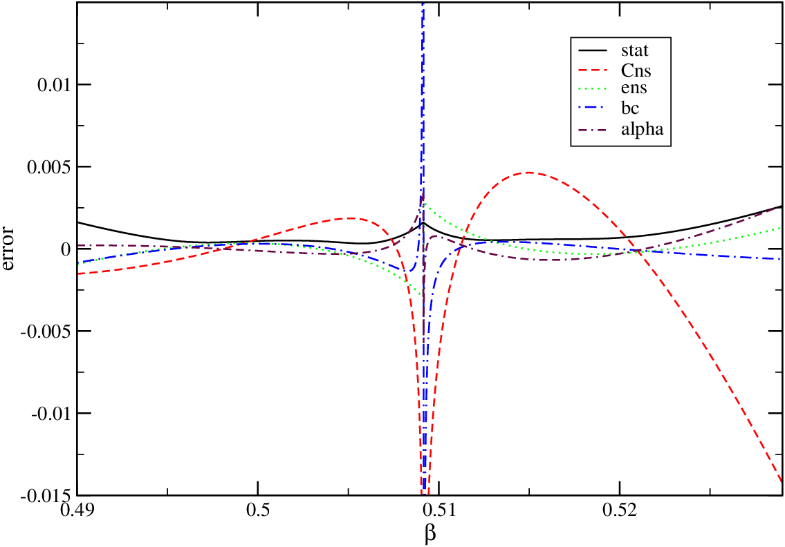
As one might expect, the differences diverge in the neighbourhood of the critical point. In the low temperature phase the largest uncertainty is due to the error of $C_{ns}$. In particular, going to the upper boundary $\beta=0.529$ of our fit interval, the uncertainty induced by the error of $C_{ns}$ rapidly increases. Therefore we decided to use the values for the specific heat obtained from the fit (29) only up to $\beta=0.525$. For larger values of $\beta$ we follow an alternative approach as discussed below. In the case of the high temperature phase we shall use the results obtained from the fit (29) down to $\beta=0.49$.

In order to complete the computation of the specific heat, we have fitted our data for the energy density with the ansatz

$$E(\beta)=\sum_{i=0}^{n}a_{i}(\beta-\beta_{0})^{i}$$

(34)

where $a_{1}$ is identified with the specific heat at $\beta_{0}$. We have included all values of $\beta$ within the interval $[\beta_{0}-\Delta,\beta_{0}+\Delta]$ into the fit. We have tested various values of $n$. Our final results are taken from fits with $n=4$. In the range $0.525<\beta_{0}\leq 0.529$ we have used $\Delta=0.008$. For $0.529<\beta_{0}<0.537$ we have used $\Delta=0.011$ and for $0.537\leq\beta_{0}\leq 0.58$ we have used $\Delta=0.016$. In all cases $\chi^{2}/$d.o.f. is close to one. To give an impression of the accuracy that is reached, we quote $C=12.690(3)$ at $\beta=0.525$ and $C=11.899(2)$ at $\beta=0.53$.

For comparison with the results obtained from the fit with ansatz (29) we have also performed fits with ansatz (34) in the range $0.522\leq\beta_{0}\leq 0.525$ using $\Delta=0.005$. The numerical results for the specific heat obtained from the two different approaches are compatible within error bars.

As we have mentioned already in the introduction, often in the literature the factor $A^{-1}\xi_{0}^{\alpha/\nu}$ is ignored when computing the finite size scaling functions $f_{1}$ and $f_{2}$. Therefore, in order to compare the results of different systems, we have to compute

$$r_{1,2}=\frac{[A\xi_{0}^{-\alpha/\nu}]_{system1}}{[A\xi_{0}^{-\alpha/\nu}]_{system2}}\;.$$

(35)

In order to fix the ratio between our definition for the specific heat of the $\phi^{4}$ model at $\lambda=2.1$ and that of experiments on ⁴He at vapour pressure, we take the ratio of our result for $A_{-}$ obtained in the previous subsection and that of [34] for the three-dimensional thermodynamic limit of ⁴He at vapor pressure. From table II of [34] we read off ⁴⁴ 4 Note that our definition of $A_{\pm}$ and that used in [34] differs by a factor of $\alpha$ $\alpha A_{-}=5.6537$. Using an alternative fit ansatz the authors get $\alpha A_{-}=5.6950$. We regard this difference as an estimate of the possible error of $\alpha A_{-}$. From the same fits, the authors obtain $\alpha=-0.01264$ and $-0.01321$, respectively. In order to match with these experimental numbers, we have taken $\alpha A_{-}=2.285$ obtained from fitting the energy density with ansatz (29), using $\alpha=-0.0127$ as input. Instead, using $\alpha=-0.0151$ we arrive at $\alpha A_{-}=2.322$. I.e. the value of $\alpha A_{-}$ is quite insensitive on the value of $\alpha$ that is assumed.

Furthermore, we need the amplitude of the correlation length for ⁴He at vapor pressure in the high and the low temperature phase. For the transversal correlation length in the low temperature phase one finds [35] and refs. therein:

$$\xi_{T}\simeq 3.42\AA\;t^{-\nu}$$

(36)

where $t=1-T/T_{\lambda}$. Alternatively we can compute the amplitudes of the correlation lengths from $A_{\pm}$ using the results for the universal amplitude ratios

$$R_{\xi}^{+}=\xi_{0,2nd}(\alpha A_{+})^{1/3}=0.3562(10)\;\;,$$

(37)

$$R_{\xi}^{-}=\xi_{0,T}(\alpha A_{-})^{1/3}=0.850(5)$$

(38)

and

$$R_{\Upsilon}=\frac{\xi_{0,2nd}}{\xi_{0,T}}=0.411(2)$$

(39)

given in [28]. To this end, we first have to convert the results for the specific heat of the experiment from $J\mbox{mole}^{-1}K^{-1}$ into $\AA^{-3}$. To this end we need the density $\rho_{\lambda}=146.1087\;\mbox{kg/m}^{3}$ [36] of ⁴He at the $\lambda$-transition and the Boltzmann constant $k_{b}=1.38065\ldots\times 10^{-23}\mbox{J/K}$. We arrive at

$$\xi_{0,T}=3.45(3)\AA$$

(40)

where we have taken into account the errors of $R_{\xi}^{-}$ and of the experimental estimate of $\alpha A_{-}$. In the case of the high temperature phase we get

$$\xi_{0,2nd}=1.422(5)\AA$$

(41)

where we have used

$$\alpha A_{+}=1.05251\times 5.6537=5.9506$$

(42)

taken from table II of [34] as input and the error is estimated by using

$$\alpha A_{+}=1.05490\times 5.6950=6.0077$$

(43)

obtained from an alternative ansatz [34].

Now we are ready to compute the ratio

$$\left(\frac{\xi_{0,^{4}He}}{\xi_{0,\phi^{4}}}\right)^{-\alpha/\nu}$$

(44)

where we can either use $\xi_{2nd}$ or $\xi_{T}$. We get $1.0386$ using $\alpha=-0.0151$ or $1.0324$ using $\alpha=-0.0127$.

Hence we arrive at

$$r_{{}^{4}He,\phi^{4}}=2.57$$

(45)

with a relative uncertainty of about $2\%$. Let us note that this number is only valid for ⁴He at vapour pressure and the $\phi^{4}$ model at $\lambda=2.1$ and the particular definitions of the specific heat that have been used.

First we performed simulations at the inverse transition temperature $\beta_{c,3D}=0.5091503(6)$ [20] of the three-dimensional system. Here the correlation length of the thin film is relatively small; we find $\xi_{2nd,film}/L_{0,eff}\approx 0.416$. Hence already rather small ratios of $L_{1}/L_{0}$ are sufficient to approximate well the two-dimensional thermodynamic limit and therefore large values of $L_{0}$ can be reached. Furthermore, by construction $L_{0}/\xi_{3D}=0$. Therefore this is an ideal location to accurately study the finite size scaling behaviour and in particular the corrections caused by free boundary conditions. At the critical point of the three-dimensional system eq. (27) reduces to

$$\frac{L_{0}}{L_{0,eff}}C(t,L_{0})=C_{ns}+cL_{0,eff}^{\alpha/\nu}+wL_{0,eff}^{-1}$$

(46)

where $C_{ns}=C_{bulk}(0)=157.9(5)$ [27] and $c=-f_{2}(0)$.

All numbers for the specific heat discussed in this section are determined by using eq. (12). As a first step, we have simulated the thickness $L_{0}=8$ for $L_{1}=L_{2}=16,24,32,48$ and $64$. We conclude from these simulations that, at the level of our statistical error, the two-dimensional thermodynamic limit of the specific heat is reached for $L_{1}=L_{2}=48$. Based on this result we performed simulations for $L_{0}=12,16,24,32,48$ and $64$ with $L_{1}=L_{2}=6L_{0}$ throughout. In all cases, we performed $10^{6}$ measurements, where for each measurement we performed one Metropolis sweep, two overrelaxation sweeps and wall cluster [37] and single cluster updates. The number of single cluster updates was chosen such that the average size of a cluster times the number of clusters is a bit less than the number of lattice sites. In total these simulations took about 5 month of CPU time on one core of a 2218 Opteron processor (2.60 GHz). The results for the specific heat, as defined by eq. (12), are summarized in table 1.

We have fitted these data with ansatz (46), where we have fixed $C_{ns}=157.9$, $\beta_{c}=0.5091503$, $\alpha=-0.0151$ and $L_{s}=1.02$. The results of these fits are summarized in table 2.

Already for $L_{0,min}=12$ the $\chi^{2}$/d.o.f. is smaller than one. Going to larger $L_{0,min}$ the statistical error of $w$ rapidly increases. Therefore we take the result obtained for $L_{0,min}=12$ as our final result. Based on our data, it is impossible to give an estimate of systematic errors due to sub-leading corrections.

In order to check the dependence on the input parameters, we have repeated the fits for $L_{0,min}=12$ using values of the input parameters that are shifted by the error of the input parameters: E.g. in one of these fits $L_{s}=1.02$ is replaced by $L_{s}=0.95$, while the other input parameters remain unchanged. In the case of $\alpha$ and $\beta_{c}$, we have taken into account the effect of the shift on $C_{ns}$ and $E_{ns}$ as given by eqs. (30,31). It turns out that shifting $L_{s}$ has the largest effect on $w$. Using $L_{s}=0.95$ we get $w=4.40(32)$. Taking the shifted value $C_{ns}=158.4$ for the analytic background we get $w=4.17(33)$. Shifting the other input parameters has less impact on the value of $w$.

Our result for $c=-f_{2}(0)$ can be compared with experiments and results obtained by field theoretic methods. On page 1028 in section V.A. of [12] the authors analyse the scaling behaviour of the specific heat of thin films at the $\lambda$-transition of the three-dimensional system. Fixing $\alpha=-0.01264$ they arrive at

$$C(0,L_{0})=[453.8\pm 4.3]-[474.0\pm 4.9]L_{0}^{-\alpha/\nu}$$

(47)

where $C$ is measured in units of $J\mbox{mole}^{-1}K^{-1}$ and $L_{0}$ in $\AA$.

Analysing our data for the specific heat at $\beta_{c,3D}$, assuming $\alpha=-0.01264$, we arrive at $c\approx-190$. Multiplying with $r_{{}^{4}He,\phi^{4}}=2.57$ we arrive at $488$ in quite good agreement with the experimental result $[474.0\pm 4.9]$, in particular when taking into account the error of $r_{{}^{4}He,\phi^{4}}$.

We can also write our result in terms of the universal ratio

$$-f_{2,R}(0)=\frac{c}{A_{+}\xi_{0,2nd}^{-\alpha/\nu}}=1.0208(2)-1.33\times(\alpha+0.0151)$$

(48)

where the error quoted in $()$ is dominated by the statistical error of the specific heat of the thin films and the uncertainty of $L_{s}$. The dependence on the value of $\alpha$ that is used in the analysis is rather weak. The authors of [13] have computed $-f_{2,R}(0)$ (in their notation $\omega_{OO}$) using $\epsilon$-expansion to $O(\epsilon)$. Their result is given in their eq. (8.17). To leading order $\omega_{OO}=1$, which is in quite good agreement with both our numerical result and with the experiment. Dohm and Sutter [17] have pointed out that the extrapolation to $\epsilon=1$ is affected by considerable ambiguities. In fact, setting $\epsilon=1$ the authors of [13] find $\omega_{OO}\approx 0.75$, (table II of [13]) which is clearly ruled out by our result as well as by experiment.

The KT phase transition occurs, up to scaling corrections, at a given value of the scaling variable $tL_{0}^{1/\nu}$ or equivalently $L_{0}/\xi_{T}$. In [10] we find $[L_{0}/\xi_{T}]^{*}=1.595(7)$. Following the KT theory [7, 8, 9] the free energy is infinitely often differentiable with respect to the temperature at the KT transition. Therefore no particular problem for the numerical analysis is expected. At the KT transition eq. (27) reduces to

$$C_{bulk}(\beta_{KT}(L_{0}))-\frac{L_{0}}{L_{0,eff}}C(\beta_{KT}(L_{0}),L_{0})=c_{KT}L_{0,eff}^{\alpha/\nu}-wL_{0,eff}^{-1}$$

(49)

where $c_{KT}$ is $f_{2}$ at $[L_{0}/\xi_{T}]^{*}=1.595(7)$.

References

- [1] Wilson K G and Kogut J, The renormalization group and the -expansion, 1974 Phys. Rep. C 12 75
- [2] Fisher M E, The renormalization group in the theory of critical behavior, 1974 Rev. Mod. Phys. 46 597
- [3] Fisher M E, Renormalization group theory: Its basis and formulation in statistical physics, 1998 Rev. Mod. Phys. 70 653
- [4] Pelissetto A and Vicari E, Critical Phenomena and Renormalization-Group Theory, 2002 Phys. Rept. 368 549 [arXiv:cond-mat/0012164]
- [5] M. N. Barber Finite-size Scaling in Phase Transitions and Critical Phenomena, Vol. 8, eds. C. Domb and J. L. Lebowitz, (Academic Press, 1983)
- [6] Finite Size Scaling and Numerical Simulation of Statistical Systems, ed. V. Privman, (World Scientific, 1990)
- [7] Kosterlitz J M and Thouless D J, Ordering, metastability and phase transitions in two-dimensional systems 1973 J. Phys. C 6 1181; Kosterlitz J M, The critical properties of the two-dimensional XY model, 1974 J. Phys. C 7 1046
- [8] José J V, Kadanoff L P, Kirkpatrick S and Nelson D R, Renormalization, vortices, and symmetry-breaking perturbations in the two-dimensional planar model, 1977 Phys. Rev. B 16 1217
- [9] Amit D J, Goldschmidt Y Y and Grinstein G, Renormalisation group analysis of the phase transition in the 2D Coulomb gas, Sine-Gordon theory and XY model, 1980 J. Phys. A 13 585
- [10] Hasenbusch M, Kosterlitz-Thouless transition in thin films: A Monte Carlo study of three-dimensional lattice models, 2009 J. Stat. Mech. P02005 [arXiv:0811.2178]
- [11] Barmatz M, Hahn I, Lipa J A, and Duncan R V, Critical phenomena in microgravity: Past, present, and future, 2007 Rev. Mod. Phys. 79 1
- [12] Gasparini F M, Kimball M O, Mooney K P, and Diaz-Avila M, Finite-size scaling of 4He at the superfluid transition, 2008 Rev. Mod. Phys. 80 1009
- [13] Krech M and Dietrich S, Free energy and specific heat of critical films and surfaces, 1992 Phys. Rev. A 46 1886
- [14] Krech M and Dietrich S, Specific heat of critical films, the Casimir force and wetting films near end points, 1992 Phys. Rev. A 46 1922
- [15] Schmolke R, Wacker A, Dohm V and Frank D, Specific Heat and Superfluid Density of Confined 4He near , 1990 Physica B 165166 575
- [16] Dohm V, The Superfluid Transition in Confined 4He: Renormalization group theory, 1993 Physica Scripta T49 46
- [17] Sutter P and Dohm V, Specific heat of confined 4He near in 3 dimensions, 1994 Physica B 194-196 613
- [18] Schultka N and Manousakis E, Scaling of the specific heat in superfluid films, 1995 Phys. Rev. Lett. 75 2710 [arXiv:cond-mat/9503116]
- [19] Nho K and Manousakis E, Heat-capacity scaling function for confined superfluids, 2003 Phys. Rev. B 68 174503 [arXiv:cond-mat/0305500]
- [20] Campostrini M, Hasenbusch M, Pelissetto A, and Vicari E, Theoretical estimates of the critical exponents of the superfluid transition in He4 by lattice methods, 2006 Phys. Rev. B 74 144506 [arXiv:cond-mat/0605083]
- [21] K. Binder, Critical behaviour at surfaces in Phase Transitions and Critical Phenomena, Vol. 8, eds. C. Domb and J. L. Lebowitz, (Academic Press, 1983) p. 1.
- [22] H. W. Diehl, Field-theoretical Approach to Critical Behaviour at Surfaces in Phase Transitions and Critical Phenomena, edited by C. Domb and J.L. Lebowitz, Vol. 10 (Academic, London 1986) p. 76.
- [23] Diehl H W, Dietrich S, and Eisenriegler E, Universality, irrelevant surface operators, and corrections to scaling in systems with free surfaces and defect planes, 1983 Phys. Rev. B 27 2937
- [24] Capehart T W and Fisher M E, Susceptibility scaling functions for ferromagnetic Ising films, 1976 Phys. Rev. B 13 5021
- [25] Hasenbusch M and Török T, High precision Monte Carlo study of the 3D XY-universality class, 1999 J. Phys. A 32 6361 [arXiv:cond-mat/9904408]
- [26] Campostrini M, Hasenbusch M, Pelissetto A, Rossi P, and Vicari E, Critical behavior of the three-dimensional XY universality class, 2001 Phys. Rev. B 63 214503 [arXiv:cond-mat/0010360]
- [27] Hasenbusch M, The three-dimensional XY universality class: A high precision Monte Carlo estimate of the universal amplitude ratio , 2006 J. Stat. Mech. P08019 [arXiv:cond-mat/0607189]
- [28] Hasenbusch M, A Monte Carlo study of the three-dimensional XY universality class: Universal amplitude ratios, 2008 J. Stat. Mech. P12006 [arXiv:0810.2716]
- [29] Fisher M E, Barber M N, and Jasnow D, Helicity Modulus, Superfluidity, and Scaling in Isotropic Systems, 1973 Phys. Rev. A 8 1111
- [30] Newman K E and Riedel E K, Critical exponents by the scaling-field method: The isotropic N-vector model in three dimensions, 1984 Phys. Rev. B 30 6615
- [31] Hasenfratz P and Leutwyler H, Goldstone Boson Related Finite Size Effects In Field Theory And Critical Phenomena With O(N) Symmetry, 1990 Nucl. Phys. B 343 241
- [32] Dimitrović I, Hasenfratz P, Nager J and Niedermayer F, Finite size effects, Goldstone bosons and critical exponents in the Heisenberg model, 1991 Nucl. Phys. B 350 893
- [33] Wolff U, Collective Monte Carlo Updating for Spin Systems, 1989 Phys. Rev. Lett. 62 361
- [34] Lipa J A, Nissen J A, Stricker D A, Swanson D R and Chui T C P, Specific heat of liquid helium in zero gravity very near the -point, 2003 Phys. Rev. B 68 174518 [arXiv:cond-mat/0310163]
- [35] Singasaas A and Ahlers G, Universality of static properties near the superfluid transition in 4He, 1984 Phys. Rev. B 30 5103
- [36] Kerr R C and Taylor R D, 1964, The molar volume and expansion coefficient of liquid 4He , Ann. Phys. 26 292
- [37] Hasenbusch M, Pinn K and Vinti S, Critical Exponents of the 3D Ising Universality Class From Finite Size Scaling With Standard and Improved Actions, 1999 Phys. Rev. B 59 11471 [arXiv:hep-lat/9806012]
- [38] Hasenbusch M, The two-dimensional XY model at the transition temperature: A high precision Monte Carlo study, 2005 J. Phys. A: Math. Gen. 38 5869 [arXiv:cond-mat/0502556]
- [39] Hasenbusch M, The Binder Cumulant at the Kosterlitz-Thouless Transition, 2008 J. Stat. Mech. P08003 [arXiv:0804.1880]
- [40] Hasenbusch M and Pinn K, Computing The Roughening Transition of Ising and Solid-on-Solid Models by BCSOS Model Matching, 1997, J. Phys. A 30 63 [cond-mat/9605019]
- [41] Kimball M O, Mehta S and Gasparini F M, Superfluid Transition of 4He for Two-Dimensional Crossover, Heat Capacity, and Finite Size Scaling, 1999, J. Low Temp. Phys. 114 467
- [42] Kimball M O, Mehta S and Gasparini F M, Specific Heat Near the Superfluid Transition of a 0.9869 micron 4He Film, 2000, J. Low Temp. Phys. 121 29
- [43]
The data are linked at the bottom of the page:
http://enthalpy.physics.buffalo.edu/Publications.html - [44] Lipa J A, Swanson D R, Nissen J A, Geng Z K, Williamson P R, Stricker D A, Chui T C P, Israelsson U E and Larson M, Specific Heat of Helium Confined to a 57-m Planar Geometry near the Lambda Point, 2000, Phys. Rev. Lett. 84 4894
- [45] Lipa J A, private communication 2009
- [46] Tam W Y and Ahlers G, Thermal conductivity of 4He I from near to K and vapor pressure to 30 bars, 1985 Phys. Rev. B 32 5932
- [47] Mohr U and Dohm V, Surface specific heat of confined 4He above and below 2000 Physica B 284-288 43
- [48] Mohr U, Kritische Spezifische Wärme in begrenzten Systemen mit Dirichlet-Oberflächen, 2000, PhD thesis, Rheinisch-Westfälische Technische Hochschule Aachen.
- [49] Dohm V, private communication
- [50] Eisenriegler E, Universal amplitude ratios for the surface-tension of polymer-solutions, 1984 J. Chem. Phys. 81 4666
- [51] Upton J P, private communication 1998, cited in [48]