Central exclusive production at high energies.Thanks: Presented at the Epihany 2009 conference: ”Hadron interactions at the dawn of the LHC”, 5-7 January 2009; dedicated to the memory of Jan Kwieciński.
Abstract
I briefly review several mechanisms of central exclusive production of mesons at high energies. Some illustrative examples for the BNL RHIC, FNAL Tevatron and CERN LHC as well as for lower energies are discussed. Some differential distributions are shown.
13.60.Le, 13.85.-t, 12.40.Nn, 12.38-t,24.85.+p,25.20.Lj,27.75.Cj,
25.75.-q
1 Introduction
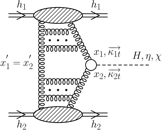
The exclusive production of mesons was studied in detail mostly close to the kinematical threshold. The Tevatron is a first accelerator which opens a possibility to study the central (semi)exclusive production of mesons at high energies. A similar program will be carried out in the future at the LHC. Here I review several mechanisms of exclusive meson production studied recently by our group (the details can be found in [1, 2, 3, 4, 5, 6, 7, 8]). In general, the mechanism of the reaction depends on the quantum numbers of the meson and/or its internal structure. For heavy scalar mesons (scalar quarkonia, scalar glueballs) the mechanism of the production, shown in Fig.1, is exactly the same as for the diffractive Higgs boson production extensively discussed in recent years by the Durham group [9]. The dominant mechanism for the exclusive heavy vector meson production is quite different. Here there are two dominant processes shown in Fig.2. When going to lower energies the mechanism of the meson production becoming more complicated and usually there exist more mechanisms. For example in Fig.3 I show a new mechanism of the glueball production proposed recently in Ref.[6].
Other exclusive or semi-exclusive processes were discussed during the conference by A. Martin [10], Ch. Royon [11] and W. Guryn [12].


2 Selected examples
Recently we have calculated differential cross sections for several exclusive processes:
- •
, ( IP IP + )
- •
(IP IP + )
- •
(IP IP)
- •
(IP IP + )
- •
(IP + IP)
- •
( IP + IP)
- •
( (IP + IR) (IP + IR))
- •
()
Above the dominant mechanisms are shown in the parantheses.
The details of the formalism as well as a detailed analysis of differential distribution in longitudinal and transverse momenta can be found in our original papers [1, 2, 3, 5, 6, 8]). Here I wish to discuss only some illustrative examples.
2.1 Exclusive production in proton-proton and proton-antiproton collisions
According to the Khoze-Martin-Ryskin approach (KMR) [9], we write the amplitude of the exclusive double diffractive color singlet production as
| (1) |
The amplitude is averaged over the color indices and over the two transverse polarizations of the incoming gluons [9].
In calculating the vertex we have included off-shellness of gluons [3]. The unintegrated gluon distributions were taken from the literature. We have demonstrated in Ref.[3] that for relatively light , unlike for the Higgs boson [9], the dominant contributions come from the nonperturbative regions of rather small gluon transverse momenta.
In Ref.[3] we have made a detailed presentation of differential distributions. Here only selected results will be shown. As an example I show distribution in Feynman variable of the meson for three different energies: W = 200 GeV (RHIC), W = 1960 GeV (Tevatron) and W = 14000 GeV (LHC) for different UGDFs from the literature. Characteristic for central diffractive production all distributions peak at 0. Although all UGDFs give a similar quality description of the low- HERA data for the structure function, they give quite different longitudinal momentum distributions of . The UGDFs which take into account saturation effects (GBW, KL) give much lower cross section than the BFKL UGDF (dash-dotted line). Therefore the process considered here would help, at least in principle, to constrain rather poorly known UGDFs.


The three-body reactions lead to correlations of outgoing protons. In Fig.5 I show an example for diffractive mechanism with KL UGDF (as an example) as well as for photon-photon fusion [3]. The () distribution obtained in the photon-photon fusion mechanism differs qualitatively from the distribution of the diffractive mechanism. One can see a strong enhancement of the cross section when , 0 which is caused by the photon propagators. Although the diffractive component is subjected to much stronger absorption effects than the electromagnetic one, it is clear that the diffractive component dominates.


The situation with the axial-vector production is new compared to both zero-spin case (scalar [3], pseudoscalar [1] mesons) as well as to the vector meson production where the vector meson is dominantly transversely polarized [2, 5], at least for small transferred four-momenta in the nucleonic line. The axial-vector meson can be polarized both transversely and longitudinally.
There is interesting theoretical aspect of the double diffractive production of the meson. The coupling vanishes for on-shell gluons (so-called Landau-Yang theorem). According to the original Landau-Yang theorem [13] the symmetries under space rotation and inversion forbid the decay of the spin-1 particle into two (on-shell) spin-1 particles (two photons, two gluons). The same is true for the fusion of two on-shell gluons. The symmetry arguments cannot be strictly applied for off-shell gluons.
In Ref.[4] we have confirmed explicitly that the Landau-Yang theorem is violated by virtual effects in diffractive production of leading to very important observational consequences. In our approach the off-shell effects are treated explicitly. For comparison, in the standard KMR approach the corresponding cross section would vanish due to their on-shell approximation. The measurement of the cross section can be therefore a good test of the off-shell effects and consequently UGDFs used in the calculation.
In Fig. 6 I show distributions in rapidity for different UGDFs from the literature. The results for different UGDFs differ significantly. The biggest cross section is obtained with BFKL UGDF and the smallest cross section with GBW UGDF. The big spread of the results is due to quite different distributions of UGDFs in gluon transverse momenta (), although when integrated over transverse momenta distributions in longitudinal momentum fraction () are fairly similar.


Comparing the left and right panels, the cross section for the axial-vector production is much smaller (about two orders of magnitude) than the cross section for the scalar production. This is related to the Landau-Yang theorem, which ”causes” vanishing of the cross section for on-shell gluons. For axial-vector quarkonia the effect is purely of off-shell nature and is due to the interplay of the off-shell matrix element and off-diagonal UGDFs. This interplay causes a huge sensitivity to UGDFs observed in Fig. 6.
At the Tevatron the mesons are measured through the decay channel. The axial-vector meson has a large branching fraction for radiative decay (BR = 0.36 [14]). This is much bigger than for the scalar where it is only about 1 % [14]. Therefore the discussed off-shell efects are very important to understand the situation in the channel observed experimentally.
2.2 Exclusive production
in proton-proton and proton-antiproton collisions
In Ref.[6] we have discussed exclusive production of scalar in the following reactions:
| (2) | |||
| (3) | |||
| (4) |
While the first process could be measured at the J-PARC complex being completed recently, the latter two reactions could be measured by the PANDA Collaboration at the new complex FAIR planned in GSI Darmstadt. The combination of these processes could shed more light on the mechanism of production as well as on its nature.


In Ref.[6] we have proposed a new mechanism (see Fig.3) which becomes dominant at lower energies. In Fig.7 we show the integrated cross section for the exclusive elastic production and for double charge exchange reaction . The thick solid line represents the pion-pion component calculated with monopole vertex form factors with = 0.8 GeV (lower) and = 1.2 GeV (upper). The difference between the lower and upper curves represents uncertainties on the pion-pion component. The pion-pion contribution grows quickly from the threshold, takes maximum at 6-7 GeV and then slowly drops with increasing energy. The gluonic contribution calculated with unintegrated gluon distributions drops with decreasing energy towards the kinematical threshold and seems to be about order of magnitude smaller than the pion-pion component at W = 10 GeV. We show the result with Kharzeev-Levin UGDF (dashed line) which includes gluon saturation effects relevant for small-x, Khoze-Martin-Ryskin UGDF (dotted line) used for the exclusive production of the Higgs boson and the result with the ”mixed prescription” (KL Gaussian) [6] for different values of the parameter: 0.5 GeV (upper thin solid line), 1.0 GeV (lower thin solid line). In the latter case results rather strongly depend on the value of the smearing parameter.
2.3 Exclusive production of
in proton-proton and proton-antiproton collisions
The photoproduction amplitude is the major building block for our prediction of exclusive production in hadronic collisions. The amplitude for the reaction under consideration is shown schematically in Fig.8.

As it is explained in Ref.[15], the imaginary part of the amplitude for the process can be written as
| (5) |
where the transverse momenta of gluons coupled to the pair can be written as
| (6) |
The quantity is the off diagonal unintegrated gluon distribution. Explicit expressions for can be found in [15]. For heavy vector mesons, helicity–flip transitions may be neglected, and we concentrate on the –channel helicity conserving amplitude, . In the forward scattering limit, i.e. for , azimuthal integrations can be performed analytically, and we obtain the following representation for the imaginary part of the amplitude for forward photoproduction :
| (7) | |||
| (8) |
where
| (9) | |||||
| (10) |
and
| (11) |
We treat the mesons as –wave states, the relevant formalism of light–cone wave functions is reviewed in [15].
The necessary formalism for the calculation of amplitudes and cross–sections was outlined in detail in Ref. [2]. Here I give only a brief summary. The basic mechanisms are shown in Fig.9.

The major difference from photoproduction at machines, where the photon was emitted by a lepton which does not participate in the strong interactions, now, both initial state hadrons can be the source of the photon. Therefore, it is now necessary to take account of the interference between two amplitudes. The photon exchange parts of the amplitude, involve only very small, predominantly transverse momentum transfers. Here we concentrate on the kinematic domain, where the outgoing protons lose only tiny fractions of their longitudinal momenta, in practice means . In terms of the transverse momenta of outgoing hadrons, , the relevant four–momentum transfers are , and and are the familiar Mandelstam variables for the appropriate subsystems. Photon virtualities are small (what counts here is that ), so that the contribution from longitudinal photons can be safely neglected. Also, as mentioned above, we assume the –channel–helicity conservation in the transition.
The Born-amplitude (without absorptive corrections) can be written in the form of a two–dimensional vector (corresponding to the two transverse (linear) polarizations of the final state vector meson):
| (12) |
Inclusion of absorptive corrections (the ’elastic rescattering’) leads in momentum space to the full, absorbed amplitude
With
| (14) |
where mb, GeV-2 were taken, the absorptive correction reads
| (15) |
The differential cross section is given in terms of as
| (16) |
where is the rapidity of the vector meson, and is the angle between and .


In Fig.10 I show the total cross section for the exclusive process as a function of the cm-energy. In the left panel I show results for two different wave functions discussed in the text: Gaussian (solid lines) and Coulomb-like (dashed lines). Free parameters of the wave function have been adjusted to reproduce the leptonic decay width in two ways: (a) using leading order formula (thin lines) and (b) inlcuding QCD corrections (thick lines). Including the –factor in the width enhances the momentum–space integral over the wave function (the WF at the spatial origin), and hence enhances the prediction for the photoproduction cross section. The ratio of the cross section for the first radial excitation to the cross section for the ground state is shown in Fig.11. The principal reason behind the suppression of the state is the well–known node effect – a cancellation of strength in the case due to the change of sign of the radial wave function. It is not surprising, that the numerical value of the –ratio is strongly sensitive to the shape of the radial light–cone wave function.


In our calculations we assumed an equality of the slopes for and production. This appears to be justified, given the large spread of predictions from different wave functions. We finally note, that the ratio depends very little on the choice of the factor (compare left and right panel).
2.4 Exclusive production of the
pairs
in proton-proton collisions
Up to now I have studied only exclusive production of a single mesons. Also the channels with meson pairs seem interesting. In particular, the channel with two charged pions which seem feasible experimentally.


The underlying mechanism was proposed long ago in Ref.[20]. The general situation is sketched in Fig.12. The corresponding amplitude for the process (with four-momenta ) can be written as
| (17) | |||||
where denotes ”interaction” between nucleon =1 (forward nucleon) or =2 (backward nucleon) and one of the two pions (3), (4). In the Regge phenomenology they can be written as:
| (18) |
Above , where is the center-of-mass energy in the (i,k) subsystem. The first terms describe the subleading reggeon exchanges while the second terms describe exchange of the leading (pomeron) trajectory. The strength parameters of the interaction are taken from Ref.[21]. More details of the calculation will be presented elsewhere [7]. The amplitude (17) is used to calculate the corresponding cross section including limitations of the four-body phase-space.

Here I wish to show only one example of the two-dimensional distribution in rapidity of positively charged pion and rapidity of negatively charged pion at the LHC energy of 14 TeV. The distribution observed differs considerably from the distribution of the phase space factor. One can see a two-dimensional shape of the ridge form elongated along the line . The minimum of the cross section on the top of the ridge occurs when and two maxima close to the phase space ends. The minimum occurs in the part of the phase space where the pomeron-pomeron contribution dominates, i.e. when both are comparable and large. The maxima are related to the dominance of the pomeron-reggeon and reggeon-pomeron mechanisms, i.e. where one of is small and the second one is large. The reggeon-reggeon contribution is completely negligible which is due to the fact that both cannot be small simultaneously. We hope that the ALICE collaboration at the LHC will be able to measure such distributions.
2.5 Exclusive
in ultrarelativistic collisions
Exclusive production of elementary particles (lepton pairs, Higgs, etc.) or mesons (vector mesons, pair of pseudoscalar mesons, etc.) in ultrarelativistic collisions is an interesting and quickly growing field [22, 23, 24] of theoretical investigation. On experimental side the situation is slightly different. So far only single- exclusive cross section was measured [25]. Here the dominant mechanism is a photon-pomeron (pomeron-photon) fusion.

Let us consider the process depicted in Fig.14. The cross section takes the familiar form of a convolution of equivalent photon fluxes and –cross sections:
| (19) |
The effective photon flux is expressed through the electric field strengths of the ions [8].
Often flux factors of equivalent, almost on-shell, photons are calculated as for point-like particles with rescaled charge , and the total cross section is calulated using a simple parton–model type formula:
| (20) |
The formulae (20) clearly does not take into account absorption effects when initial nuclei undergo nuclear breakup. This can be easily done in the impact parameter space where the geometry of the collision is more explicit. Then rather two-dimensional flux factors [26] must be used.
The simple EPA formula can be generalized to
| (21) |
Here an extra function was introduced which excludes those cases when nucler collisions, leading to nuclear breakup, take place (). The two-dimensional fluxes in (21) can be calculated in terms of the charge form factor of nucleus [28] as:
| (22) |
where the auxiliary function reads:
| (23) |
The second ingredient of our approach is cross section. Here the situation is not well established. The cross section for this process was measured up to = 4 GeV [29]. At low energy one observes a huge increase of the cross section.
In Fig.15 we have collected the world data (see [29] and references therein). We use rather directly experimental data in order to evaluate the cross section in nucleus-nucleus collisions. In Fig.15 we show our fit to the world data .

The cross section above = 4 GeV was never measured in the past. It is well known that the cross section for hadrons can be well described in the VDM-Regge type model. We use a similar approach for the final state channel . In Fig.15 we present the corresponding -integrated cross section together with existing experimental data taken from [29]. The vanishing of the VDM-Regge cross section at is due to , limitations. It is obvious from Fig.15 that the VDM-Regge model cannot explain the huge close-to-threshold enhancement. In Fig.16 we show distribution of the cross section for the nucleus-nucleus scattering in photon-photon center-of-mass energy for both low-energy component and high-energy VDM-Regge component. Below = 2 GeV the low-energy component dominates. The situation reverses above = 2 GeV. One can study the high energy component imposing extra cut on . However, the cross section drops quickly with increasing invariant mass of two- mesons.

For illustration in Fig.17 we show the model distribution in impact parameter . We show distributions for the low- and high-energy components separately. I also show distributions for point-like charge, monopole form factor and realistic charge density (see [8]). One can see slightly different results for different approaches how to calculate flux factors of equivalent photons.

Finally in Fig.18 I show distribution in rapidity of the pair. Compared to the point-like case, the distribution obtained with realistic charge density is concentrated at midrapidities, and configurations when both ’s are in very forward or both ’s are in very backward directions are strongly damped compared to the case with point-like nucleus charges. One can also see a difference between results obtained with an approximate monopole form factor and with the exact one calculated from realistic charge density.


3 Conclusions
We have derived, for the first time in the literature, QCD amplitude for exclusive elastic double diffractive production of axial-vector meson. According to the Landau-Yang theorem the amplitude vanishes for the fusion of on-shell gluons. We have generalized the formalism proposed recently for diffractive production of the Higgs boson and derived corresponding vertex function. The predicted total cross section, obtained from the bare amplitude is of the order of a fraction of nb, depending on the model of UGDF. This is about two orders of magnitude less than a similar cross section for .
However, because the branching fraction , one may expect a different situation in the channel. This is similar as for inclusive production of P-wave quarkonia, where the signal (in the channel) of is of similar size as that for .
We have calculated the forward amplitude for reaction within the formalism of -factorization. In this approach the energy dependence of the process is encoded in the -dependence of unintegrated gluon distributions. The latter object is constrained by data on inclusive deep inelastic scattering. The -dependence for the process involves a free parameter and is parametrized. We have used different Ansätze for the wave functions. The results for production depend only slightly on the model of the wave function, while the ratio shows a substantial sensitivity. We compared our results for the total cross section with a recent data from HERA. Our results are somewhat lower than data, although the overall discrepancy is not worrysome, given the large uncertainties due to the rather poor experimental resolution in the meson mass. The amplitudes for the process are used next to calculate the amplitude for the reaction assuming the photon-Pomeron (Pomeron-photon) underlying dynamics. We have calculated several differential distributions including soft absorption effects not included so far in the literature. Our predictions are relevant for current experiments at the Tevatron.
For the first time in the literature we have estimated the cross section for exclusive meson (glueball candidate) production not far from the threshold. We have included both gluon induced diffractive mechanism and the pion-pion exchange contributions.
The first component was obtained by extrapolating down the cross section in the Khoze-Martin-Ryskin approach with unintegrated gluon distributions from the literature as well as using two-gluon impact factor approach. A rather large uncertainties are associated with the diffractive component. At present only upper limit can be obtained for the diffractive component as the decay coupling constant remains unknown. The coupling constant could be extracted only in high-energy exclusive production of where other mechanisms are negligible.
The calculation of the meson-exchange contribution requires introducing extra vertex form factors. At largest PANDA energies they are relatively well known and the pion-pion fusion can be reliably calculated. We predict the dominance of the pion-pion contribution close to the threshold. Our calculation shows that the diffractive component is by more than order of magnitude smaller than the pion-pion fusion component in the energy region of the future PANDA experiments. The diffractive component may dominate over the pion-pion component only for center-of-mass energies 15 GeV. Clearly an experimental program is required to disentagle the reaction mechanism.
We have made first estimate of the exclusive production of pairs of charged pions at high-energy. Different combinations of pomeron-reggeon fusion were included. Rather large cross sections are predicted at RHIC, Tevatron and LHC. Here I have shown only rapidity distributions of pions at LHC. The production of the two pions is strongly correlated in the () space. Even at relatively high energies the inclusion of reggeon exchanges is crucial as amplitudes with different combination of exchanges interfere or/and subsystem energies can be relatively small 10 GeV. At high-energies we find a preference for the same hemisphere (same-sign rapidity) emission of and . For example at LHC energies the same hemisphere emission constitutes about 90 % of all cases.
We have calculated, for the first time, realistic cross sections for exclusive production in ultrarelativistic heavy-ion collisions at RHIC. We have used realistic charge densities to calculate the nuclear charge form factors. The absorption effects have been included.
It was shown that calculating both flux factors and realistically is necessary to make reliable etimates of the nucleus-nucleus exclusive production of the pairs. Large cross sections, of the order of fraction of milibarn, have been found. The bulk of the cross section is, however, concentrated in low photon-photon energies (low invariant masses)
The mesons, decaying into , can be measured e.g. by the STAR detector at RHIC and the ALICE detector at LHC.
Acknowledgments The collaboration with Wolfgang Schäfer, Roman Pasechnik, Oleg Teryaev, Anna Cisek, Mariola Kłusek and Piotr Lebiedowicz on the topics presented here is acknowledged. This work was partially supported by the Polish Ministry of Science and Higher Education under grants no. N N202 249235 and N N202 078735.
References
- [1] A. Szczurek, R. Pasechnik and O. Teryaev, hep-ph/0608302, Phys. Rev. D75, 054021 (2007).
- [2] W. Schäfer and A. Szczurek, Arxiv:0705.2887, Phys. Rev. D76, 094014 (2007).
- [3] R. Pasechnik, A. Szczurek and O. Teryaev, Arxiv:0709.0857, Phys. Rev. D78 014007 (2008).
- [4] R. Pasechnik, A. Szczurek and O. Teryaev, Arxiv:0901.4187.
- [5] A. Rybarska, W. Schäfer and A. Szczurek, Arxiv:0805.0717, Phys. Lett. B668 126 (2008).
- [6] A. Szczurek and P. Lebiedowicz, Arxiv:0806.4896.
- [7] P. Lebiedowicz and A. Szczurek, in preparation.
- [8] M. Kłusek, W. Schäfer and A. Szczurek, Phys. Lett. B674 (2009) 92.
- [9]
V.A. Khoze, A.D. Martin and M.G. Ryskin, Phys. Lett. B 401,
330 (1997);
V.A. Khoze, A.D. Martin and M.G. Ryskin, Eur. Phys. J. C 23, 311 (2002). - [10] A. Martin, these proceedings.
- [11] Ch. Royon, these proceedings.
- [12] W. Guryn, these proceedings.
- [13]
L.D. Landau, Dokl. Akad. Nauk. USSR 60 (1948) 207;
C.N. Yang, Phys. Rev. 17 (1950) 242. - [14]
W. M. Yao et al. (Particle Data Group), Jour. Phys.
G33 1 (2006),
C. Amsler et al. (Particle Data Group), Phys. Lett. B667 1 (2008). - [15] I. P. Ivanov, N. N. Nikolaev and A. A. Savin, Phys. Part. Nucl. 37, 1 (2006).
- [16] I. P. Ivanov and N. N. Nikolaev, Phys. Rev. D 65, 054004 (2002).
- [17] J. Breitweg et al. [ZEUS Collaboration], Phys. Lett. B 437, 432 (1998).
- [18] C. Adloff et al. [H1 Collaboration], Phys. Lett. B 483, 23 (2000).
- [19] I. Rubinskiy for the H1 and ZEUS Collaborations, “Exclusive Processes in ep collision at HERA”, a talk at the International Europhysics Conference On High Energy Physics (EPS-HEP2007), Manchester, England, 19-25 July 2007.
- [20] J. Pumplin and F.S. Henyey, Nucl. Phys. B117 (1976) 377.
- [21] A. Donnachie and P.V. Landshoff, Phys. Lett. B296 (1992) 227.
- [22] V.M. Budnev, I.F. Ginzburg, G.V. Meledin and V.G. Serbo, Phys. Rep. 15 (1975) 181.
- [23] G. Baur, K. Hencken, D. Trautmann, S. Sadovsky and Y. Kharlov, Phys. Rep. 364 (2002) 359.
- [24] K. Hencken et al., Phys. Rep. 458 (2008) 1.
- [25] B. Grube et al. (STAR collaboration), arXiv:0808.3991 [nucl-ex].
- [26] J.D. Jackson, Classical Electrodynamics, 2nd ed. (Wiley, New York, 1975), p. 722.
- [27] V.P. Goncalves and M.V.T. Machado, Eur. Phys. J. C29 (2003) 271; V.P. Goncalves, M.V.T. Machado and W.K. Sauter, Eur. Phys. J. C46 (2006) 219.
- [28] G. Baur and L.G. Ferreiro Filho, Phys. Lett. B254 (1991) 30.
- [29] D. Morgan, M.R. Pennington and M.R. Whalley, J. Phys. G20 Suppl. 8A (1994) A1-A147.