跳到论文正文
W Papers独立论文阅读器 arXiv:0904.1481 论文正文 计算阅读时间 · 0%
引用这篇论文根据当前论文元数据生成,正式投稿前建议核对。


License: arXiv.org perpetual non-exclusive license
arXiv:0904.1481v1 [math-ph] 09 Apr 2009

Spectrum in multi-species asymmetric simple exclusion process on a ring

Chikashi Arita ††thanks: Faculty of Mathematics, Kyushu University    Atsuo Kuniba ††thanks: Institute of Physics, University of Tokyo    Kazumitsu Sakai    Tsuyoshi Sawabe ††thanks: Data Mining Division, Mathematical Systems, Inc.
April 9, 2009
Abstract

The spectrum of Hamiltonian (Markov matrix) of a multi-species asymmetric simple exclusion process on a ring is studied. The dynamical exponent concerning the relaxation time is found to coincide with the one-species case. It implies that the system belongs to the Kardar-Parisi-Zhang or Edwards-Wilkinson universality classes depending on whether the hopping rate is asymmetric or symmetric, respectively. Our derivation exploits a poset structure of the particle sectors, leading to a new spectral duality and inclusion relations. The Bethe ansatz integrability is also demonstrated.

1 Introduction

In recent years, intensive studies on non-equilibrium phenomena have been undertaken through a variety of stochastic process models of many particle systems [S1]. Typical examples are driven lattice gas systems with a simple but nonlinear interaction among constituent particles. The asymmetric simple exclusion process (ASEP) is one of the simplest driven lattice gas models proposed originally to describe the dynamics of ribosome along RNA [MGP]. In the ASEP, each site is occupied by at most one particle. Each particle is allowed to hop to its nearest neighbor right (left) site with the rate pp (q)(q) if it is empty. The ASEP admits exact analyses of non-equilibrium properties by the matrix product ansatz and the Bethe ansatz. The matrix product form of the stationary state was first found in the open boundary case [DEHP]. Similar results have been obtained in various driven lattice gas systems in one dimension with both open and periodic boundary conditions [BE]. Applications of the Bethe ansatz [B] to the ASEP have also been successful. See for example the works [GS, K], [S2] and [DE] for the studies of the ASEP under periodic, infinite and open boundary conditions, respectively. In the periodic boundary case, the dynamical exponent zz of the relaxation time to the stationary state is z=3/2z=3/2 if p≠qp\neq q and z=2z=2 if p=qp=q according to the analysis of the Bethe equation. This implies that the ASEP belongs to the Kardar-Parisi-Zhang (KPZ) or Edwards-Wilkinson (EW) universality classes depending on whether the hopping rate is asymmetric or symmetric, respectively.

In this paper we consider the following multi-species generalization of the ASEP on a ring of length LL. A local state on each site of the ring assumes NN states 1,2,…,N1,2,\ldots,N. A nearest neighbor pair of the states is interchanged with the transition rate

α​β→β​α​{pif ​α>β,qif ​α<β.\displaystyle\alpha\beta\to\beta\alpha\;\;\begin{cases}p&\text{if }\alpha>\beta,\\ q&\text{if }\alpha<\beta.\end{cases}

We regard the local state α=1\alpha=1 as a vacant site and α=2,…,N\alpha=2,\ldots,N as a site occupied by a particle of the α\alphath kind. The dynamics is formulated in terms of the master equation dd​t​|P⁡(t)⟩=H​|P⁡(t)⟩\frac{d}{dt}|P(t)\rangle=H|P(t)\rangle on the probability vector |P⁡(t)⟩|P(t)\rangle. We call the model the (N−1N\!-\!1)-species ASEP or simply the multi-species ASEP. The usual ASEP corresponds to N=2N=2.

The NL×NLN^{L}\times N^{L} Markov matrix HH will be called the “Hamiltonian” although it is not Hermitian for p≠qp\neq q. (At p=qp=q, it is Hermitian and coincides with the s​l​(N)sl(N) invariant Heisenberg Hamiltonian.) Its eigenvalue with the largest real part is 0 corresponding to the stationary state. The other eigenvalues contribute to the relaxation behavior through |P⁡(t)⟩=et​H​|P⁡(0)⟩|P(t)\rangle={\rm e}^{tH}|P(0)\rangle. Especially those with the second largest real part determine the relaxation time τ\tau and the dynamical exponent zz by the scaling behavior τ∼Lz\tau\sim L^{z}. Our finding is that zz remains the same with the usual ASEP N=2N=2. The key to the result is that the spectrum of HH in any multi-species particle sector includes that for an N=2N=2 sector. We systematize such spectral inclusion relations by exploiting the poset structure of particle sectors. As a byproduct we find a duality, a global aspect in the spectrum of the Hamiltonian, which is new even at the Heisenberg point p=qp=q.

There are some other multi-species models with different hopping rules such as ABC model [EKKM] and AHR model [AHR, RSS], etc. The recent paper [KN] says that the AHR model still has the dynamical exponent z=3/2z=3/2. The multi-species ASEP in this paper is a most standard generalization of the one-species ASEP allowing the application of the Bethe ansatz. Let us comment on this point and related works to clarify the origin of integrability of the model. In [AR], a formulation by Hecke algebra was given for a wider class of stochastic models including reaction-diffusion systems. A Bethe ansatz treatment was presented in [AB]. As is well known [Ba], however, there underlies a two dimensional integrable vertex model behind a Bethe ansatz solvable Hamiltonian. In the present model, the relevant vertex model is a special case of the Perk-Schultz model (called “second class of models” in [PS]). It should be fair to say that the nested Bethe ansatz for the present model is originally due to Schultz [Sc]. For an account of the Perk-Schultz RR-matrix in the framework of multi-parameter quantum group, see [OY] and reference therein.

The layout of the paper is as follows. In section 2, we introduce the multi-species ASEP Hamiltonian together with its basic properties. In section 3, we explain how the spectral gap responsible for the relaxation time is reduced to the one-species case and determine the dynamical exponent as in (3.17). Our argument is based on spectral inclusion property (3.11) and conjecture 3.1 supported by numerical analyses. In section 4, we elucidate a new duality of the spectrum of the Hamiltonian in theorem 4.12. An intriguing feature is that it emerges only by dealing with all the basic sectors of the N=LN=L-state model on the length LL ring. (The term “basic sector” will be defined in section 2.) The argument of section 4 is independent from the Bethe ansatz. In section 5, we discuss the Bethe ansatz integrability of the multi-species ASEP and the underlying vertex model including the completeness issue. We execute the nested algebraic Bethe ansatz in an arbitrary nesting order, which leads to an alternative explanation of the spectral inclusion property. Except the arbitrariness of the nesting order, section 5.1.1 is a review.

Appendix A gives a proof of the dimensional duality (theorem 4.9) needed in section 4. Appendix B is a sketch of a derivation of the stationary state by the Bethe ansatz. Appendix C contains the complete spectra of transfer matrix and Hamiltonian in the basic sectors with the corresponding Bethe roots for (p,q)=(23,13)(p,q)=(\frac{2}{3},\frac{1}{3}) and L=4L=4. They agree with the completeness conjectures in section 5.1.2.

2 Multi-species ASEP

2.1 Master equation

Consider an LL-site ring ℤL{\mathbb{Z}}_{L} where each site i∈ℤLi\in{\mathbb{Z}}_{L}, is assigned with a variable (local state) ki∈{1,…,N}​(N≥1)k_{i}\in\{1,\ldots,N\}\,(N\geq 1). We introduce a stochastic model on ℤL{\mathbb{Z}}_{L} such that nearest neighbor pairs of local states (α,β)=(ki,ki+1)(\alpha,\beta)=(k_{i},k_{i+1}) are interchanged with the transition rate:

α​β→β​α​{pif ​α>β,qif ​α<β,\displaystyle\alpha\beta\to\beta\alpha\;\;\begin{cases}p&\text{if }\alpha>\beta,\\ q&\text{if }\alpha<\beta,\end{cases} (2.1)

where pp and qq are real nonnegative parameters. More precisely, the dynamics is formulated in terms of the continuous-time master equation on the probability of finding the configuration (k1,…,kL)(k_{1},\dots,k_{L}) at time tt:

dd​t​P​(k1,…,kL,t)=∑i∈ℤLΘ⁡(ki+1−ki)​P​(k1,…,ki−1,ki+1,ki,ki+2,…,kL,t)−∑i∈ℤLΘ(ki−ki+1)P(k1,…,kL;t),\displaystyle\begin{split}\frac{d}{dt}P(k_{1},\dots,k_{L};t)&=\sum_{i\in{\mathbb{Z}}_{L}}\Theta(k_{i+1}-k_{i})P(k_{1},\dots,k_{i-1},k_{i+1},k_{i},k_{i+2},\dots,k_{L};t)\\ &-\sum_{i\in{\mathbb{Z}}_{L}}\Theta(k_{i}-k_{i+1})P(k_{1},\dots,k_{L};t),\end{split} (2.2)

where Θ\Theta is a step function defined as

Θ⁡(x)={p(x>0),0(x=0),q(x<0).\displaystyle\Theta(x)=\begin{cases}p&(x>0),\\ 0&(x=0),\\ q&(x<0).\end{cases} (2.3)

(Actually, Θ⁡(0)\Theta(0) can be set to any value.)

Our model can be regarded as an interacting multi-species particle system on the ring. We interpret the local state ki=αk_{i}=\alpha as representing the site ii occupied by a particle of the α\alphath kind. The transition (2.1) is viewed as a local hopping process of particles. We identify the first kind particles with vacancies. Note that a particle α\alpha has been assumed to overtake any β(<α)\beta(<\alpha) with the same rate pp as the vacancy β=1\beta=1.

We call this model the multi-species ASEP or more specifically the (N−1)(N\!-\!1)-species ASEP. The usual ASEP corresponds to N=2N=2. We will be formally concerned with the zero-species ASEP (N=1N=1) as well. The case p=qp=q will be called the multi-species symmetric simple exclusion process (SSEP).

Let |1⟩,…,|N⟩|1\rangle,\ldots,|N\rangle be the basis of the single-site space ℂN{\mathbb{C}}^{N} and represent a particle configuration (k1,…,kL)(k_{1},\dots,k_{L}) as the ket vector |k1,…,kL⟩=|k1⟩⊗⋯⊗|kL⟩∈(ℂN)⊗L|k_{1},\dots,k_{L}\rangle=|k_{1}\rangle\otimes\cdots\otimes|k_{L}\rangle\in({\mathbb{C}}^{N})^{\otimes L}. In terms of the probability vector

|P(t)⟩=∑1≤ki≤NP(k1,…,kL;t)|k1,…,kL⟩,\displaystyle|P(t)\rangle=\sum_{1\leq k_{i}\leq N}P(k_{1},\dots,k_{L};t)|k_{1},\dots,k_{L}\rangle, (2.4)

the master equation (2.2) is expressed as

dd​t​|P⁡(t)⟩=H​|P⁡(t)⟩,\displaystyle\frac{d}{dt}|P(t)\rangle=H|P(t)\rangle, (2.5)

where the linear operator HH has the form

H\displaystyle H =∑i∈ℤLhi,i+1,\displaystyle=\sum_{i\in{\mathbb{Z}}_{L}}h_{i,i+1}, (2.6)
h\displaystyle h =∑1≤α<β≤N(−pEβ​β⊗Eα​α−qEα​α⊗Eβ​β+pEα​β⊗Eβ​α+qEβ​α⊗Eα​β).\displaystyle=\sum_{1\leq\alpha<\beta\leq N}(-pE_{\beta\beta}\otimes E_{\alpha\alpha}-qE_{\alpha\alpha}\otimes E_{\beta\beta}+pE_{\alpha\beta}\otimes E_{\beta\alpha}+qE_{\beta\alpha}\otimes E_{\alpha\beta}). (2.7)

Here hi,i+1h_{i,i+1} acts on the iith and the (i+1)(i\!+\!1)th components of the tensor product as hh and as the identity elsewhere. Eα​βE_{\alpha\beta} denotes the NN by NN matrix unit sending |γ⟩|\gamma\rangle to δγ​β​|α⟩\delta_{\gamma\beta}|\alpha\rangle.

The equation (2.5) has the form of the Schrödinger equation with imaginary time and thus provides our multi-species ASEP with a quantum Hamiltonian formalism. Of course in the present case, P⁡(k1,…,kL,t)P(k_{1},\dots,k_{L};t) itself gives the probability distribution unlike the squared wave functions in the case of quantum mechanics. Nevertheless we call the matrix HH the Hamiltonian11 1 A more proper terminology is Markov matrix. in this paper by the abuse of language.

2.2 Basic properties of Hamiltonian

Our Hamiltonian HH is an NLN^{L} by NLN^{L} matrix whose off-diagonal elements are p,qp,q or 00, and diagonal elements belong to p​ℤ≤0+q​ℤ≤0p{\mathbb{Z}}_{\leq 0}+q{\mathbb{Z}}_{\leq 0}. Each column of HH sums up to 00 assuring the conservation of the total probability ∑1≤ki≤NP⁡(k1,…,kL,t)\sum_{1\leq k_{i}\leq N}P(k_{1},\dots,k_{L};t). It enjoys the symmetries

[H,C]=0,R​H​R−1=Q​H​Q−1=H|p↔q.\displaystyle[H,C]=0,\quad RHR^{-1}=QHQ^{-1}=H|_{p\leftrightarrow q}. (2.8)

where C,RC,R and QQ are linear operators defined by

C|k1,…,kL⟩\displaystyle C|k_{1},\ldots,k_{L}\rangle =|kL,k1,…,kL−1⟩\displaystyle=|k_{L},k_{1},\ldots,k_{L-1}\rangle (cyclic shift),\displaystyle(\text{cyclic shift}), (2.9)
R|k1,…,kL⟩\displaystyle R|k_{1},\ldots,k_{L}\rangle =|kL,kL−1,…,k1⟩\displaystyle=|k_{L},k_{L-1},\ldots,k_{1}\rangle (reflection),\displaystyle(\text{reflection}), (2.10)
Q|k1,…,kL⟩\displaystyle Q|k_{1},\ldots,k_{L}\rangle =|N+−k1,…,N+−kL⟩\displaystyle=|N\!+\!1\!-\!k_{1},\ldots,N\!+\!1\!-\!k_{L}\rangle (“charge conjugation”)\displaystyle(\text{``charge conjugation"}) (2.11)

satisfying CL=R2=Q2=1C^{L}=R^{2}=Q^{2}=1. HH is Hermitian only at p=qp=q, where it becomes the Hamiltonian of the s​l​(N)sl(N)-invariant Heisenberg spin chain H=p​∑i∈ℤL(σi,i+1−1)H=p\sum_{i\in{\mathbb{Z}}_{L}}(\sigma_{i,i+1}-1) with σi,i+1\sigma_{i,i+1} being the transposition of the local states ki↔ki+1k_{i}\leftrightarrow k_{i+1}. In general, imaginary eigenvalues of HH form complex conjugate pairs. In section 5, Bethe ansatz integrability of HH for general p,qp,q will be demonstrated. Although HH is not normal in general, we expect that it is diagonalizable based on conjecture 5.1 and the remark following it. This fact will be used only in corollary 4.8.

In view of the transition rule (2.1), our Hamiltonian HH obviously preserves the number of particles of each kind. It follows that the space of states (ℂN)⊗L({\mathbb{C}}^{N})^{\otimes L} splits into a direct sum of sectors and HH has the block diagonal structure:

(ℂN)⊗L\displaystyle({\mathbb{C}}^{N})^{\otimes L} =⨁mV(m),V(m)=⨁{ki}​ in sector ​mℂ|k1,…,kL⟩,\displaystyle=\bigoplus_{m}V(m),\quad V(m)=\bigoplus_{\{k_{i}\}\text{ in sector }\,m}{\mathbb{C}}|k_{1},\ldots,k_{L}\rangle, (2.12)
H\displaystyle H =⨁mH⁡(m),H⁡(m)∈End​V​(m).\displaystyle=\bigoplus_{m}H(m),\quad H(m)\in{\rm End}\,V(m). (2.13)

Here the direct sums ⨁m\bigoplus_{m} extend over m=(m1,…,mN)∈ℤ≥0Nm=(m_{1},\ldots,m_{N})\in{\mathbb{Z}}_{\geq 0}^{N} such that m1+⋯+mN=Lm_{1}+\cdots+m_{N}=L. The array mm labels a sector V⁡(m)V(m), which is a subspace of (ℂN)⊗L({\mathbb{C}}^{N})^{\otimes L} specified by the multiplicities of particles of each kind. Namely, the latter sum in (2.12) is taken over all (k1,…,kL)∈{1,…,N}L(k_{1},\ldots,k_{L})\in\{1,\ldots,N\}^{L} such that

Sort(k1,…,kL)=1​…​1⏞m12​…​2⏞m2⋯N​…​N⏞mN,\displaystyle\text{Sort}(k_{1},\ldots,k_{L})=\overbrace{1...1}^{m_{1}}\overbrace{2...2}^{m_{2}}\cdots\overbrace{N...N}^{m_{N}}, (2.14)

where Sort stands for the ordering non decreasing to the right. In other words, the {ki}\{k_{i}\} in (2.12) runs over all the permutations of the right hand side of (2.14). The array mm itself will also be called a sector. A sector, m=(2,0,4,1,0,3)m=(2,0,4,1,0,3) for instance, will also be referred in terms of the Sort sequence as 12​34​463=11333346661^{2}3^{4}46^{3}=1133334666. By the definition dimV⁡(m)=L!/∏i=1Nmi!\dim V(m)=L!/\prod_{i=1}^{N}m_{i}!.

By now we have separated the master equation (2.5) into the ones in each sector dd​t​|P⁡(t)⟩=H⁡(m)​|P⁡(t)⟩\frac{d}{dt}|P(t)\rangle=H(m)|P(t)\rangle with |P⁡(t)⟩∈V⁡(m)|P(t)\rangle\in V(m). Since the transition rule (2.1) only refers to the alternatives α>β\alpha>\beta or α<β\alpha<\beta, the master equation in the sector 12​34​4631^{2}3^{4}46^{3} for example is equivalent to that in a2​b4​c​d3a^{2}b^{4}c\,d^{3} for any ≤a<b<c<d≤N1\!\leq\!a\!<\!b\!<\!c\!<\!d\!\leq\!N.

Henceforth without loss of generality we take N=LN=L and restrict our consideration to the basic sectors that have the form m=(m1,…,mn,0,…,0)m=(m_{1},\ldots,m_{n},0,\ldots,0) for some nn with m1,…,mnm_{1},\ldots,m_{n} being all positive. The basic sectors are labeled with the elements of the set

ℳ\displaystyle{\mathcal{M}} ={(m1,…,mn)∈ℤ≥1n∣1≤n≤L,m1+⋯+mn=L}.\displaystyle=\{(m_{1},\ldots,m_{n})\in{\mathbb{Z}}_{\geq 1}^{n}\mid 1\leq n\leq L,\,m_{1}+\cdots+m_{n}=L\}. (2.15)

In this convention, which will be employed in the rest of the paper except section 5, nn plays the role of NN in the sense that H⁡(m)H(m) for m=(m1,…,mn)∈ℳm=(m_{1},\ldots,m_{n})\in{\mathcal{M}} is equivalent to the Hamiltonian of the (n−1)(n-1)-species ASEP.

In section 3 we study specific eigenvalues of HH that are relevant to the leading behavior of the relaxation. In section 4 we elucidate a spectral duality, a new global aspect of the spectrum of HH, which has escaped a notice in earlier works mostly devoted to the studies of the thermodynamic limit L→∞L\rightarrow\infty under a fixed NN.

3 Relaxation to the stationary state

3.1 General remarks

The initial value problem of the master equation dd​t​|P⁡(t)⟩=H⁡(m)​|P⁡(t)⟩\frac{d}{dt}|P(t)\rangle=H(m)|P(t)\rangle with |P⁡(t)⟩∈V⁡(m)|P(t)\rangle\in V(m) in the sector m=(m1,…,mn)∈ℳm=(m_{1},\ldots,m_{n})\in{\mathcal{M}} (2.15) is formally solved as

|P⁡(t)⟩=et​H​(m)​|P⁡(0)⟩.\displaystyle|P(t)\rangle={\rm e}^{tH(m)}|P(0)\rangle. (3.1)

There is a unique stationary state corresponding to the zero eigenvalue of H⁡(m)H(m). The stationary state has a non-uniform probability distribution [PEM] except for the zero-species, the one-species and the SSEP cases, where P⁡(k1,…,kL)=1/dimV⁡(m)P(k_{1},\dots,k_{L})=1/\dim V(m). All the other eigenvalues of H⁡(m)H(m) have strictly negative real parts, which are responsible for various relaxation modes to the stationary state. (The associated eigenvectors themselves are not physical probability vectors having non-negative components.) Let us denote by |P⁡(∞)⟩|P(\infty)\rangle the stationary state. In general, the system exhibits the long time behavior

|P(t)⟩−|P(∞)⟩∼e−t/τ(t→∞),\displaystyle|P(t)\rangle-|P(\infty)\rangle\sim{\rm e}^{-t/\tau}\quad(t\rightarrow\infty), (3.2)

where τ\tau is the relaxation time. An important characteristic of the non-equilibrium dynamics is the scaling property of the relaxation time with respect to the system size:

τ∼Lz(L→∞),\displaystyle\tau\sim L^{z}\quad(L\rightarrow\infty), (3.3)

where zz is the dynamical exponent. The thermodynamic limit L→∞L\rightarrow\infty is to be taken under the fixed densities ρj=mj/L\rho_{j}=m_{j}/L for j=1,…,nj=1,\ldots,n. (Recall L=m1+⋯+mnL=m_{1}+\cdots+m_{n} in (2.15), therefore ρ1+⋯+ρn=1\rho_{1}+\cdots+\rho_{n}=1.)

The spectrum in a sector m∈ℳm\in{\mathcal{M}} will be denoted by

Spec⁡(m)=multiset of eigenvalues of​H​(m),\displaystyle{\rm Spec}(m)=\text{multiset of eigenvalues of}\,H(m), (3.4)

where the multiplicities counts the degrees of degeneracy. Spec⁡(m){\rm Spec}(m) is invariant under complex conjugation. The charge conjugation property (2.11) implies the symmetry

Spec⁡(m1,…,mn)=Spec⁡(mn,…,m1).\displaystyle{\rm Spec}(m_{1},\ldots,m_{n})={\rm Spec}(m_{n},\ldots,m_{1}). (3.5)

We say that a complex eigenvalue xx of H⁡(m)H(m) is larger (smaller) than yy if Re⁡(x)>Re⁡(y){\rm Re}(x)>{\rm Re}(y) (Re⁡(x)<Re⁡(y){\rm Re}(x)<{\rm Re}(y)). Spec⁡(m){\rm Spec}(m) contains 00 as the unique largest eigenvalue. For a finite LL, we say an eigenvalue EE of H⁡(m)H(m) is second largest if

Re​E=max⁡Re⁡(Spec⁡(m)∖{0}).\displaystyle{\rm Re}\,E=\max{\rm Re}({\rm Spec}(m)\setminus\{0\}). (3.6)

From (3.1) and (3.2), the scaling property (3.3) is equivalent to the following behavior of the second largest eigenvalues

max⁡Re⁡(Spec⁡(m)∖{0})=−c​L−z+o⁡(L−z)(L→∞)\displaystyle\max{\rm Re}({\rm Spec}(m)\setminus\{0\})=-cL^{-z}+o(L^{-z})\quad(L\rightarrow\infty) (3.7)

if the initial condition |P⁡(0)⟩|P(0)\rangle is generic. Here c>0c>0 is an “amplitude” which can depend on ρ1,…,ρn\rho_{1},\ldots,\rho_{n} in general, but not on LL.

In the remainder of this section, we derive the exponent zz of the multi-species ASEP based on (3.7). Our argument reduces the problem essentially to the one-species case and is partly based on a conjecture supported by numerical analyses.

3.2 Known results on the one-species ASEP

In this subsection we review the known results on the one-species ASEP. Thus we shall exclusively consider the sector of the form m=(m1,m2)∈ℳm=(m_{1},m_{2})\in{\mathcal{M}}, and regard the local states 11 and 22 as vacancies and the particles of one kind, respectively. Recall also that L=m1+m2L=m_{1}+m_{2}.

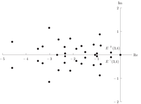
The second largest eigenvalues are known to form a complex-conjugate pair, which will be denoted by E±​(m)E^{\pm}(m). See figure 1. When m1=m2m_{1}=m_{2} or p=qp=q, the degeneracy E+​(m)=E−​(m)∈ℝE^{+}(m)=E^{-}(m)\in{\mathbb{R}} occurs.

Refer to caption
Figure 1: Spec⁡(3,4){\rm Spec}(3,4) for (p,q)=(0.8,0.2).(p,q)=(0.8,0.2).

In [GS, K, GM], the large LL asymptotic form

E±​((1−ρ)​L,ρ​L)=±2​π​i​|(p−q)​(1−2​ρ)|​L−1−2​C​|p−q|​ρ⁡(1−ρ)​L−32+O⁡(L−2)\displaystyle E^{\pm}((1-\rho)L,\rho L)=\pm 2\pi{\rm i}|(p-q)(1-2\rho)|L^{-1}-2C|p-q|\sqrt{\rho(1-\rho)}L^{-\frac{3}{2}}+O(L^{-2}) (3.8)

with a fixed particle density ρ=m2/L\rho=m_{2}/L was derived for p≠qp\neq q by an analysis of the Bethe equation. The two terms are both invariant under ρ↔1−ρ\rho\leftrightarrow 1-\rho. The constant CC has been numerically evaluated as C=6.50918933794​…C=6.50918933794\ldots . Thus from (3.7) the one-species ASEP for p≠qp\neq q has the dynamical exponent z=32z=\frac{3}{2}, which is a characteristic value for the Kardar-Parisi-Zhang universality class [KPZ].

In the SSEP case p=qp=q, the Hamiltonian H⁡(m1,m2)H(m_{1},m_{2}) is Hermitian, hence all the eigenvalues are real. The system relaxes to the equilibrium stationary state. For a finite LL, the second largest eigenvalues take the simple form

E+​(m1,m2)=E−​(m1,m2)=−4​p​sin2⁡(πL)(0<m2<L),\displaystyle E^{+}(m_{1},m_{2})=E^{-}(m_{1},m_{2})=-4p\sin^{2}(\frac{\pi}{L})\quad(0<m_{2}<L), (3.9)

which is independent of the density ρ=m2/L\rho=m_{2}/L as long as 0<ρ<10<\rho<1. The asymptotic behavior in L→∞L\to\infty is easily determined as

E±​((1−ρ)​L,ρ​L)=−4​π2​p​L−2+O⁡(L−4),\displaystyle E^{\pm}((1-\rho)L,\rho L)=-4\pi^{2}pL^{-2}+O(L^{-4}), (3.10)

which is free from a contribution of order L−32L^{-\frac{3}{2}}. From (3.10), we find the dynamical exponent z=2z=2, which is the characteristic value for the Edwards-Wilkinson universality class [EW].

3.3 Eigenvalues of 𝑯⁡(𝟐,𝟏,𝟑,𝟏)H(2,1,3,1) -an example

Let us proceed to the multi-species ASEP. Before considering a general sector in the next subsection, we illustrate characteristic features of the spectrum along an example. Figure 2 (a) is a plot (black dots) of the spectrum Spec⁡(2,1,3,1){\rm Spec}(2,1,3,1) on the complex plane. We recall that the sector (2,1,3,1)(2,1,3,1) means the ring of length 7 populated with 4 kinds of particles with multiplicities 2,1,32,1,3 and 11, among which the first kind ones are regarded as vacancies.

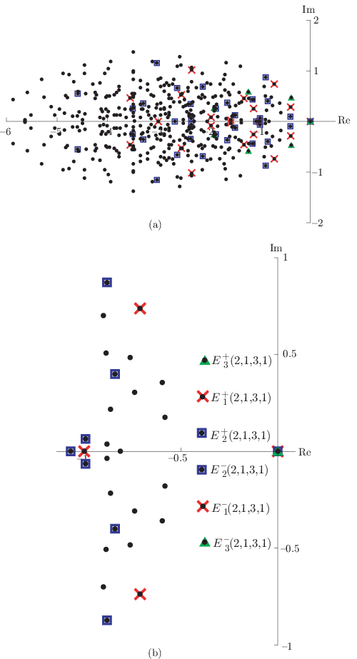
For comparison, we have also included the plot of the spectra in the one-species sectors (2,5)(2,5), (3,4)(3,4) and (6,1)(6,1) in different colors and shapes. These one-species sectors are related to the multi-species sector (2,1,3,1)(2,1,3,1) as follows. The sector (2,5)=(2,1+3+1)(2,5)=(2,1+3+1) is obtained by identification of all kinds of particles (except for vacancies) as one kind of particles. The sector (3,4)=(2+1,3+1)(3,4)=(2+1,3+1) is obtained by identification of the second kind particles as vacancies and the rest of particles as one kind of particles. The sector (6,1)=(2+1+3,1)(6,1)=(2+1+3,1) is obtained by identification of the second and the third kinds of particles as vacancies. In figure 2 (a), we observe that all the colored dots overlap the black dots. Namely, Spec⁡(2,5),Spec⁡(3,4),Spec⁡(6,1){\rm Spec(2,5)},\,{\rm Spec(3,4)},\,{\rm Spec(6,1)} are totally embedded into Spec⁡(2,1,3,1){\rm Spec}(2,1,3,1).

Figure 2 (b) shows that the second largest eigenvalues (denoted by Ej±​(2,1,3,1)E^{\pm}_{j}(2,1,3,1)) in those one-species sectors form a string within Spec⁡(2,1,3,1){\rm Spec}(2,1,3,1) near the origin. Although their real parts are not strictly the same, there is no black dot between the string and the origin. More precisely, there is no eigenvalue in the sector (2,1,3,1)(2,1,3,1) which is nonzero and larger than any second largest eigenvalues in the one-species sectors (2,5)(2,5), (3,4)(3,4) and (6,1)(6,1). This property is a key to our argument in the sequel.
Refer to caption
Figure 2: (a) Spec⁡(2,1,3,1){\rm Spec}(2,1,3,1) (black dot), Spec⁡(2,5){\rm Spec}(2,5) (red ×\times), Spec⁡(3,4){\rm Spec}(3,4) (blue square) and Spec⁡(6,1){\rm Spec}(6,1) (green triangle) with (p,q)=(0.8,0.2)(p,q)=(0.8,0.2). (b) An enlarged view near the origin.

3.4 Eigenvalues of multi-species ASEP

Let us systematize the observations made in the previous subsection. First we claim that the following inclusion relation holds generally:

Spec⁡(m1,…,mn)⊃Spec⁡(m1+⋯+mj,mj+1+⋯+mn)(1≤j≤n−1).\displaystyle{\rm Spec}(m_{1},\dots,m_{n})\supset{\rm Spec}(m_{1}+\cdots+m_{j},m_{j+1}+\cdots+m_{n})\quad(1\leq j\leq n-1). (3.11)

Each one-species sector appearing in the right-hand side of (3.11) is obtained by the identification similar to the previous subsection:

∘⋯∘⏞m1​|⋯|​∘⋯∘⏞mj⏟m1+⋯+mj|∘⋯∘⏞mj+1​|⋯|​∘⋯∘⏞mn⏟mj+1+⋯+mn.\displaystyle\underbrace{\overbrace{\circ\cdots\circ}^{m_{1}}|\cdots|\overbrace{\circ\cdots\circ}^{m_{j}}}_{m_{1}+\cdots+m_{j}}|\underbrace{\overbrace{\circ\cdots\circ}^{m_{j+1}}|\cdots|\overbrace{\circ\cdots\circ}^{m_{n}}}_{m_{j+1}+\cdots+m_{n}}.

The relation (3.11) is a special case of the more general statement in theorem 4.5. See also section 5.2.1 for an account from the nested Bethe ansatz.

Next we introduce a class of eigenvalues of H⁡(m)H(m) for a multi-species sector m=(m1,…,mn)∈ℳm=(m_{1},\ldots,m_{n})\in{\mathcal{M}} by

Ej±​(m)=E±​(m1+⋯+mj,mj+1+⋯+mn)(1≤j≤n−1),\displaystyle E^{\pm}_{j}(m)=E^{\pm}(m_{1}+\cdots+m_{j},m_{j+1}+\cdots+m_{n})\quad(1\leq j\leq n-1), (3.12)

where E±E^{\pm} in the right hand side are the second largest eigenvalues in the one-species sector introduced in section 3.2. In view of (3.11), we know Ej±​(m)∈Spec⁡(m)E^{\pm}_{j}(m)\in{\rm Spec}(m). Note that Re⁡(Ej+​(m))=Re⁡(Ej−​(m)){\rm Re}(E^{+}_{j}(m))={\rm Re}(E^{-}_{j}(m)), but the subscript jj does not necessarily reflect the ordering of the eigenvalues with respect to their real parts. Generalizing the previous observation on figure 2, we make

Conjecture 3.1.

In any sector m=(m1,…,mn)∈ℳm=(m_{1},\dots,m_{n})\in{\mathcal{M}}, there is no eigenvalue E∈Spec⁡(m)E\in{\rm Spec}(m) such that

max⁡{Re​E1±​(m),…,Re​En−1±​(m)}<Re​E<0.\displaystyle\max\{{\rm Re}\,E^{\pm}_{1}(m),\ldots,{\rm Re}\,E^{\pm}_{n-1}(m)\}<{\rm Re}\,E<0. (3.13)

The one-species case n=2n=2 is trivially true by the definition. So far the conjecture has been checked in all the sectors mm satisfying dimV⁡(m)<8000\dim V(m)<8000.

Admitting the conjecture, we are able to claim that the second largest eigenvalues in Spec⁡(m){\rm Spec}(m) are equal to Ej±​(m)E^{\pm}_{j}(m) for some 1≤j≤n−11\leq j\leq n-1. (Such jj may not be unique.) The asymptotic behavior of Ej±​(m)E^{\pm}_{j}(m) is derived from (3.8) and (3.12) as

Ej±​(ρ1​L,…,ρn​L)=±2​π​i​|(p−q)​(1−2​rj)|​L−1−2​C​|p−q|​rj​(1−rj)​L−32+O⁡(L−2)\displaystyle\begin{split}&E^{\pm}_{j}(\rho_{1}L,\dots,\rho_{n}L)\\ &=\pm 2\pi{\rm i}|(p-q)(1-2r_{j})|L^{-1}-2C|p-q|\sqrt{r_{j}(1-r_{j})}L^{-\frac{3}{2}}+O(L^{-2})\end{split} (3.14)

for p≠qp\neq q, where rj=ρ1+⋯+ρjr_{j}=\rho_{1}+\cdots+\rho_{j} is fixed. We remark that the leading terms in (3.14) depend on jj only through rjr_{j} in the amplitudes. We call the eigenvalues E1±​(m),…,En−1±​(m)E^{\pm}_{1}(m),\ldots,E^{\pm}_{n-1}(m) next leading. Thus the second largest eigenvalues are next leading. All the next leading eigenvalues possess the same asymptotic behavior as the second largest ones up to the amplitudes as far as the first 2 leading terms in (3.14) are concerned.

With regard to the SSEP case p=qp=q, the stationary state is an equilibrium state. H⁡(m)H(m) is Hermitian and Ej±​(m)E^{\pm}_{j}(m) is real. We have the following explicit form as in the one-species case:

E1±​(m)=⋯=En−1±​(m)=−4​p​sin2⁡(πL).\displaystyle E_{1}^{\pm}(m)=\cdots=E_{n-1}^{\pm}(m)=-4p\sin^{2}(\frac{\pi}{L}). (3.15)

In other words, the next leading eigenvalues Ej±​(m)E_{j}^{\pm}(m) are degenerated in the SSEP limit p−q→0p-q\to 0. See figure 3, where the string of the next leading eigenvalues shrinks to a point on the real axis as p−qp-q approaches 00.

Refer to caption
Figure 3: Degeneracy in the SSEP limit p−q→0p-q\to 0 in the sector (2,1,3,1)(2,1,3,1). (p,q)(p,q) is taken as (a) (0.8,0.2)(0.8,0.2), (b) (0.7,0.3)(0.7,0.3), (c) (0.6,0.4)(0.6,0.4) and (d) (0.5,0.5)(0.5,0.5).

As the one-species case (3.10), we find

Ej±​(ρ1​L,…,ρn​L)=−4​π2​p​L−2+O⁡(L−4).\displaystyle E^{\pm}_{j}(\rho_{1}L,\dots,\rho_{n}L)=-4\pi^{2}pL^{-2}+O(L^{-4})\ . (3.16)

To summarize, the results (3.14) and (3.16) lead to the following behavior of the relaxation time τ\tau:

τ∼{L32for ​p≠q,L2for ​p=q,(L→∞).\displaystyle\tau\sim\begin{cases}L^{\frac{3}{2}}&\text{for }\;p\neq q,\\ L^{2}&\text{for }\;p=q,\end{cases}\quad(L\rightarrow\infty). (3.17)

Therefore we conclude that the dynamical exponent of the multi-species ASEP is independent of the number of species. It belongs to the KPZ universality class (z=32z=\frac{3}{2}) for p≠qp\neq q, and to the EW universality class (z=2z=2) for p=qp=q.

We leave it as a future study to investigate the gap between the next leading eigenvalues and further smaller eigenvalues, which governs the pre-asymptotic behavior of the multi-species ASEP.

4 Duality in Spectrum

Throughout this section, a sector means a basic sector as promised in section 2.2. We fix the number of sites in the ring L∈ℤ≥2L\in{\mathbb{Z}}_{\geq 2}. Our goal is to prove theorem 4.12, which exhibits a duality in the spectrum of Hamiltonian.

4.1 Another label of sectors

Set

Ω\displaystyle\Omega ={1,2,…,L−1},\displaystyle=\{1,2,\ldots,L-1\}, (4.1)
𝒮\displaystyle{\mathcal{S}} =the power set of ​Ω.\displaystyle=\text{the power set of }\Omega. (4.2)

Recall that the sectors in the length LL chain are labeled with the set ℳ{\mathcal{M}} (2.15). We identify ℳ{\mathcal{M}} with 𝒮{\mathcal{S}} by the one to one correspondence:

ℳ∋m=(m1,…,mn)⟷{s1<⋯<sn−1}=𝔰∈𝒮\displaystyle{\mathcal{M}}\ni m=(m_{1},\ldots,m_{n})\longleftrightarrow\{s_{1}<\cdots<s_{n-1}\}={\mathfrak{s}}\in{\mathcal{S}} (4.3)

specified via sj=m1+m2+⋯+mjs_{j}=m_{1}+m_{2}+\cdots+m_{j}, namely,

∘⋯∘⏞m1⏟s1|∘⋯∘⏞m2⏟s2|⋯⏟sn−1|∘⋯∘⏞mn,\displaystyle\underbrace{\underbrace{\underbrace{\overbrace{\circ\cdots\circ}^{m_{1}}}_{s_{1}}|\overbrace{\circ\cdots\circ}^{m_{2}}}_{s_{2}}|\cdots}_{s_{n-1}}|\overbrace{\circ\cdots\circ}^{m_{n}},

where the numbers of the symbols ∘\circ and || are LL and n−1n-1, respectively. For example the identification ℳ↔𝒮{\mathcal{M}}\leftrightarrow{\mathcal{S}} for L=4L=4 is given as follows:

(1,1,1,1)↔{1,2,3}(1,1,1,1)\leftrightarrow\{1,2,3\}

(1,1,2)↔{1,2}(1,2,1)↔{1,3}(2,1,1)↔{2,3}(1,1,2)\leftrightarrow\{1,2\}\quad(1,2,1)\leftrightarrow\{1,3\}\quad(2,1,1)\leftrightarrow\{2,3\}

(1,3)↔{1}(2,2)↔{2}(3,1)↔{3}(1,3)\leftrightarrow\{1\}\quad(2,2)\leftrightarrow\{2\}\quad(3,1)\leftrightarrow\{3\}

(4)↔∅(4)\leftrightarrow\emptyset.

An element of 𝒮{\mathcal{S}} will also be called a sector. In the remainder of this section we will mostly work with the label 𝒮{\mathcal{S}} instead of ℳ{\mathcal{M}}. There are ♯​𝒮=2L−1\sharp{\mathcal{S}}=2^{L-1} distinct sectors. We employ the notation:

𝔰¯=Ω∖𝔰=complement sector of ​𝔰.\displaystyle\overline{\mathfrak{s}}=\Omega\setminus\mathfrak{s}=\text{complement sector of }\,\mathfrak{s}. (4.4)

For a sector 𝔰={s1<⋯<sn−1}∈𝒮\mathfrak{s}=\{s_{1}<\cdots<s_{n-1}\}\in{\mathcal{S}}, we introduce the set 𝒫⁡(𝔰){\mathcal{P}}(\mathfrak{s}) by (see (2.14))

𝒫(𝔰)={k=(k1,…,kL)∣Sort(k)=1​…​1⏞s12​…​2⏞s2−s1⋯n−1​…​n−1⏞sn−1−sn−2n​…​n⏞L−sn−1},\displaystyle{\mathcal{P}}(\mathfrak{s})=\{k=(k_{1},\ldots,k_{L})\mid\text{Sort}(k)=\overbrace{1...1}^{s_{1}}\overbrace{2...2}^{s_{2}-s_{1}}\cdots\overbrace{n\!-\!1...n\!-\!1}^{s_{n-1}-s_{n-2}}\!\overbrace{n...n}^{L-s_{n-1}}\}, (4.5)

where Sort stands for the ordering non decreasing to the right as in (2.14). For 𝔰=∅∈𝒮\mathfrak{s}=\emptyset\in{\mathcal{S}}, this definition should be understood as 𝒫⁡(∅)={(1,…,1)}{\mathcal{P}}(\emptyset)=\{(1,\ldots,1)\}.

To each sector we associate the bra and ket vector spaces

V𝔰∗=⨁k∈𝒫⁡(𝔰)ℂ⟨k1,…,kL|,V𝔰=⨁k∈𝒫⁡(𝔰)ℂ|k1,…,kL⟩.\displaystyle V_{\mathfrak{s}}^{\ast}=\bigoplus_{k\in{\mathcal{P}}(\mathfrak{s})}{\mathbb{C}}\langle k_{1},\ldots,k_{L}|,\quad V_{\mathfrak{s}}=\bigoplus_{k\in{\mathcal{P}}(\mathfrak{s})}{\mathbb{C}}|k_{1},\ldots,k_{L}\rangle. (4.6)

Here k1,…,kL∈{1,…,L}k_{1},\ldots,k_{L}\in\{1,\ldots,L\} stand for local states. For example if L=3L=3, one has

V∅\displaystyle V_{\emptyset} =ℂ​|111⟩,\displaystyle={\mathbb{C}}|111\rangle,
V{1}\displaystyle V_{\{1\}} =ℂ⁡|122⟩⊕ℂ⁡|212⟩⊕ℂ⁡|221⟩,\displaystyle={\mathbb{C}}|122\rangle\oplus{\mathbb{C}}|212\rangle\oplus{\mathbb{C}}|221\rangle,
V{2}\displaystyle V_{\{2\}} =ℂ⁡|112⟩⊕ℂ⁡|121⟩⊕ℂ⁡|211⟩,\displaystyle={\mathbb{C}}|112\rangle\oplus{\mathbb{C}}|121\rangle\oplus{\mathbb{C}}|211\rangle,
VΩ=V{1,2}\displaystyle V_{\scriptscriptstyle\Omega}=V_{\{1,2\}} =ℂ⁡|123⟩⊕ℂ⁡|132⟩⊕ℂ⁡|213⟩⊕ℂ⁡|231⟩⊕ℂ⁡|312⟩⊕ℂ⁡|321⟩.\displaystyle={\mathbb{C}}|123\rangle\oplus{\mathbb{C}}|132\rangle\oplus{\mathbb{C}}|213\rangle\oplus{\mathbb{C}}|231\rangle\oplus{\mathbb{C}}|312\rangle\oplus{\mathbb{C}}|321\rangle.

Note that the vectors like |222⟩|222\rangle and |113⟩|113\rangle are not included in any V𝔰V_{\mathfrak{s}} because we are concerned with basic sectors only. See (4.5). In general, one has

dimV𝔰=dimV𝔰∗=L!s1!(s2−s1)!⋯(sn−1−sn−2)!(L−sn−1)!\displaystyle\dim V_{\mathfrak{s}}=\dim V_{\mathfrak{s}}^{\ast}=\frac{L!}{s_{1}!(s_{2}\!-\!s_{1})!\cdots(s_{n-1}\!-\!s_{n-2})!(L\!-\!s_{n-1})!} (4.7)

for 𝔰={s1<⋯<sn−1}∈𝒮\mathfrak{s}=\{s_{1}<\cdots<s_{n-1}\}\in{\mathcal{S}}.

Suppose ℳ∋m↔𝔰∈𝒮{\mathcal{M}}\ni m\leftrightarrow{\mathfrak{s}}\in{\mathcal{S}} under the correspondence (4.3). We renew the symbols H⁡(m)H(m) and V⁡(m)V(m) in (2.12)–(2.13) as

V𝔰=V⁡(m),H𝔰=H⁡(m).\displaystyle V_{\mathfrak{s}}=V(m),\quad H_{\mathfrak{s}}=H(m). (4.8)

The set 𝒮{\mathcal{S}} is equipped with the natural poset (partially ordered set) structure with respect to ⊆\subseteq. The poset structure is encoded in the Hasse diagram [St], which is useful in our working below. In the present case, it is just the L−1L\!-\!1 dimensional hypercube, where each vertex corresponds to a sector. Sectors are so arranged that every edge of the hypercube becomes an arrow 𝔰→𝔱\mathfrak{s}\rightarrow\mathfrak{t} meaning that 𝔰⊂𝔱\mathfrak{s}\subset\mathfrak{t} and ♯​𝔱=♯​𝔰+1\sharp\mathfrak{t}=\sharp\mathfrak{s}+1. There is the unique sink corresponding to the maximal sector Ω∈𝒮\Omega\in{\mathcal{S}} and the unique source corresponding to the minimal sector ∅∈𝒮\emptyset\in{\mathcal{S}}. See figure 4.

Refer to caption
Figure 4: Hasse diagrams (a), (b), (c) and (d) for L=2,3,4L=2,3,4 and 55, respectively. Sectors are labeled by 𝒮{\mathcal{S}} (4.2) as well as the sequence Sort⁡(k){\rm Sort}(k) of local states as in (4.5).

We introduce the natural bilinear pairing between the bra and ket vectors by

⟨k1,…,kL|j1,…,jL⟩=δk1,j1⋯δkL,jL.\displaystyle\langle k_{1},\ldots,k_{L}|j_{1},\ldots,j_{L}\rangle=\delta_{k_{1},j_{1}}\cdots\delta_{k_{L},j_{L}}. (4.9)

With respect to the pairing, V𝔰∗V_{\mathfrak{s}}^{\ast} and V𝔱V_{\mathfrak{t}} are dual if 𝔰=𝔱\mathfrak{s}=\mathfrak{t} and orthogonal if 𝔰≠𝔱\mathfrak{s}\neq\mathfrak{t}.

Any linear operator G→\overset{\rightarrow}{G} acting on ket vectors give rise to the unique linear operator G←\overset{\leftarrow}{G} acting on bra vectors via (⟨k1,…,kL|G←)|j1,…,jL⟩=⟨k1,…,kL|(G→|j1,…,jL⟩)\left(\langle k_{1},\ldots,k_{L}|\overset{\leftarrow}{G}\right)|j_{1},\ldots,j_{L}\rangle=\langle k_{1},\ldots,k_{L}|\left(\overset{\rightarrow}{G}|j_{1},\ldots,j_{L}\rangle\right) and vice versa. We write this quantity simply as ⟨k1,…,kL​|G|​j1,…,jL⟩\langle k_{1},\ldots,k_{L}|G|j_{1},\ldots,j_{L}\rangle as usual, and omit ←\overset{\leftarrow}{\phantom{e}} and →\overset{\rightarrow}{\phantom{e}} unless an emphasis is preferable. The transpose GTG^{\rm T} of GG is defined by ⟨k|GT|j⟩=⟨j|G|k⟩(=:Gj​k)\langle k|G^{\rm T}|j\rangle=\langle j|G|k\rangle\;(=:G_{jk}) for any k=(k1,…,kL)k=(k_{1},\ldots,k_{L}) and j=(j1,…,jL)j=(j_{1},\ldots,j_{L}). Of course G→T\overset{\rightarrow}{G}{}^{\rm T} is equivalent to G←\overset{\leftarrow}{G} in the sense that

GT​|k⟩=∑jGk​j​|j⟩,⟨k|​G=∑jGk​j​⟨j|.\displaystyle G^{\rm T}|k\rangle=\sum_{j}G_{kj}|j\rangle,\quad\langle k|G=\sum_{j}G_{kj}\langle j|. (4.10)

4.2 Operator 𝝋𝖘,𝖙\varphi_{\mathfrak{s},\mathfrak{t}}

Let 𝔰,𝔱∈𝒮\mathfrak{s},\mathfrak{t}\in{\mathcal{S}} be sectors such that 𝔰⊆𝔱\mathfrak{s}\subseteq\mathfrak{t}. We introduce a ℂ{\mathbb{C}}-linear operator φ𝔰,𝔱\varphi_{\mathfrak{s,t}} in terms of its action on ket vectors φ→𝔰,𝔱:V𝔱→V𝔰\overset{\rightarrow}{\varphi}_{\mathfrak{s},\mathfrak{t}}:V_{\mathfrak{t}}\rightarrow V_{\mathfrak{s}}. We define φ𝔰,𝔰\varphi_{\mathfrak{s},\mathfrak{s}} to be the identity operator for any sector 𝔰\mathfrak{s}. Before giving the general definition of the case 𝔰⊂𝔱\mathfrak{s}\subset\mathfrak{t}, we illustrate it with the example 𝔰={2,5}⊂𝔱={2,3,5,8}\mathfrak{s}=\{2,5\}\subset\mathfrak{t}=\{2,3,5,8\} with L=9L=9. The Sort sequence of the local states in the sense of (4.5) for 𝒫⁡(𝔱){\mathcal{P}}(\mathfrak{t}) and 𝒫⁡(𝔰){\mathcal{P}}(\mathfrak{s}) read as follows:

𝒫⁡(𝔱={2,3,5,8}):11​|2​2​|3​33​|5​444​|8​5,𝒫⁡(𝔰={2,5}):11​|2​2 2 2​|5​3 3 3 3.\displaystyle\begin{split}{\mathcal{P}}(\mathfrak{t}=\{2,3,5,8\}):&\quad 11\overset{2}{|}2\overset{3}{|}33\overset{5}{|}444\overset{8}{|}5,\\ {\mathcal{P}}(\mathfrak{s}=\{2,5\}):&\quad 11\overset{2}{|}2\,2\,2\overset{5}{|}3\,3\,3\,3.\end{split} (4.11)

According to these lists, we define φ𝔰,𝔱{\varphi}_{\mathfrak{s},\mathfrak{t}} to be the operator replacing the local states as 3→2,4→3,5→33\rightarrow 2,4\rightarrow 3,5\rightarrow 3 (keeping 11 and 22 unchanged) within all the ket vectors |k1,…,kL⟩|k_{1},\ldots,k_{L}\rangle in V𝔱V_{\mathfrak{t}}.

General definition of φ𝔰,𝔱{\varphi}_{\mathfrak{s},\mathfrak{t}} is similar and goes as follows. Suppose 𝔱={t1<⋯<tn}\mathfrak{t}=\{t_{1}<\cdots<t_{n}\} and 𝔰=𝔱∖{ti1,…,til}\mathfrak{s}=\mathfrak{t}\setminus\{t_{i_{1}},\ldots,t_{i_{l}}\}. Then φ𝔰,𝔱{\varphi}_{\mathfrak{s},\mathfrak{t}} is a ℂ{\mathbb{C}}-linear operator determined by its action on base vectors as follows:

φ→𝔰,𝔱:V𝔱⟶V𝔰|k1,…,kL⟩↦|k′1,…,k′L⟩,\displaystyle\begin{array}[]{cccc}\overset{\rightarrow}{\varphi}_{\mathfrak{s},\mathfrak{t}}:&V_{\mathfrak{t}}&\longrightarrow&V_{\mathfrak{s}}\\ &|k_{1},\ldots,k_{L}\rangle&\mapsto&|k^{\prime}_{1},\ldots,k^{\prime}_{L}\rangle,\end{array}

where x′=x−♯⁡{ij∣ij<x}x^{\prime}=x-\sharp\{i_{j}\mid i_{j}<x\}.

Example 4.1.
|ϕ⟩:\displaystyle|\phi\rangle: =|21433⟩−|12343⟩∈V𝔱​(𝔱={1,2,4},L=5),\displaystyle=|21433\rangle-|12343\rangle\in V_{\mathfrak{t}}\;\;\;(\mathfrak{t}=\{1,2,4\},\;L=5),
φ12,124​|ϕ⟩\displaystyle{\varphi}_{12,124}|\phi\rangle =|21333⟩−|12333⟩,{φ1,12​φ12,124​|ϕ⟩=|21222⟩−|12222⟩,φ2,12​φ12,124​|ϕ⟩=0,\displaystyle=|21333\rangle-|12333\rangle,\;\;\begin{cases}{\varphi}_{1,12}\,{\varphi}_{12,124}|\phi\rangle=|21222\rangle-|12222\rangle,\\ {\varphi}_{2,12}\,{\varphi}_{12,124}|\phi\rangle=0,\end{cases}
φ14,124​|ϕ⟩\displaystyle{\varphi}_{14,124}|\phi\rangle =|21322⟩−|12232⟩,{φ1,14​φ14,124​|ϕ⟩=|21222⟩−|12222⟩,φ4,14​φ14,124​|ϕ⟩=|11211⟩−|11121⟩,\displaystyle=|21322\rangle-|12232\rangle,\;\;\begin{cases}{\varphi}_{1,14}\,{\varphi}_{14,124}|\phi\rangle=|21222\rangle-|12222\rangle,\\ {\varphi}_{4,14}\,{\varphi}_{14,124}|\phi\rangle=|11211\rangle-|11121\rangle,\end{cases}
φ24,124​|ϕ⟩\displaystyle{\varphi}_{24,124}|\phi\rangle =|11322⟩−|11232⟩,{φ2,24​φ24,124​|ϕ⟩=0,φ4,24​φ24,124​|ϕ⟩=|11211⟩−|11121⟩,\displaystyle=|11322\rangle-|11232\rangle,\;\;\begin{cases}{\varphi}_{2,24}\,{\varphi}_{24,124}|\phi\rangle=0,\\ {\varphi}_{4,24}\,{\varphi}_{24,124}|\phi\rangle=|11211\rangle-|11121\rangle,\end{cases}
φ1,124​|ϕ⟩\displaystyle{\varphi}_{1,124}|\phi\rangle =|21222⟩−|12222⟩,\displaystyle=|21222\rangle-|12222\rangle,
φ4,124​|ϕ⟩\displaystyle{\varphi}_{4,124}|\phi\rangle =|11211⟩−|11121⟩,\displaystyle=|11211\rangle-|11121\rangle,
φ2,124​|ϕ⟩\displaystyle{\varphi}_{2,124}|\phi\rangle =0,φ∅,124​|ϕ⟩=0,\displaystyle=0,\quad{\varphi}_{\emptyset,124}|\phi\rangle=0,

where φ12,124{\varphi}_{12,124} is an abbreviation of φ{1,2},{1,2,4}{\varphi}_{\{1,2\},\{1,2,4\}}, etc.

The following property of φ𝔰,𝔱{\varphi}_{\mathfrak{s},\mathfrak{t}} is a direct consequence of the definition.

Lemma 4.2.

For a pair of sectors 𝔰⊂𝔱\mathfrak{s}\subset\mathfrak{t}, let 𝔰0⊂𝔰1⊂⋯⊂𝔰l\mathfrak{s}_{0}\subset\mathfrak{s}_{1}\subset\cdots\subset\mathfrak{s}_{l} be any sectors such that 𝔰0=𝔰,𝔰l=𝔱\mathfrak{s}_{0}=\mathfrak{s},\mathfrak{s}_{l}=\mathfrak{t} and ♯​𝔰j+1=♯​𝔰j+1\sharp\mathfrak{s}_{j+1}=\sharp\mathfrak{s}_{j}+1 for all 0≤j<l0\leq j<l. Then,

φ𝔰,𝔱=φ𝔰,𝔰1φ𝔰1,𝔰2⋯φ𝔰l−1,𝔱.\displaystyle{\varphi}_{\mathfrak{s},\mathfrak{t}}={\varphi}_{\mathfrak{s},\mathfrak{s}_{1}}\,{\varphi}_{\mathfrak{s}_{1},\mathfrak{s}_{2}}\cdots{\varphi}_{\mathfrak{s}_{l-1},\mathfrak{t}}.

In particular, the composition in the right hand side is independent of the choice of the intermediate sectors 𝔰1,…,𝔰l−1\mathfrak{s}_{1},\ldots,\mathfrak{s}_{l-1}.

In example 4.1, one can observe, for instance, φ4,124​|ϕ⟩=φ4,14​φ14,124​|ϕ⟩=φ4,24​φ24,124​|ϕ⟩{\varphi}_{4,124}|\phi\rangle={\varphi}_{4,14}\,{\varphi}_{14,124}|\phi\rangle={\varphi}_{4,24}\,{\varphi}_{24,124}|\phi\rangle.

Let us turn to the transpose φ𝔰,𝔱T\varphi_{\mathfrak{s},\mathfrak{t}}^{\rm T}. By the definition (see (4.10)), we have

φ→𝔰,𝔱T:V𝔰⟶V𝔱|k1,…,kL⟩↦∑j∈𝒫⁡(𝔱)′|j1,…,jL⟩,\displaystyle\begin{array}[]{cccc}\overset{\rightarrow}{\varphi}_{\mathfrak{s},\mathfrak{t}}\!\!\!\!{}^{\rm T}:&V_{\mathfrak{s}}&\longrightarrow&V_{\mathfrak{t}}\\ &|k_{1},\ldots,k_{L}\rangle&\mapsto&\displaystyle\sum_{j\in{\mathcal{P}}(\mathfrak{t})}\!\!{}^{\prime}\;|j_{1},\ldots,j_{L}\rangle,\end{array}

where Σ′\Sigma^{\prime} extends over those j=(j1,…,jL)∈𝒫⁡(𝔱)j=(j_{1},\ldots,j_{L})\in{\mathcal{P}}(\mathfrak{t}) such that φ𝔰,𝔱|j1,…,jL⟩=|k1,…,kL⟩{\varphi}_{\mathfrak{s},\mathfrak{t}}|j_{1},\ldots,j_{L}\rangle=|k_{1},\ldots,k_{L}\rangle. For example in example 4.1, one has

φ14,124T​|21322⟩=|21433⟩+|31423⟩+|31432⟩.\displaystyle\varphi^{\rm T}_{14,124}|21322\rangle=|21433\rangle+|31423\rangle+|31432\rangle.

From (4.2) and (4.2) it follows that φ𝔰,𝔱​φ𝔰,𝔱T=dimV𝔱dimV𝔰​Id\varphi_{\mathfrak{s},\mathfrak{t}}\,\varphi^{\rm T}_{\mathfrak{s},\mathfrak{t}}=\frac{\dim V_{\mathfrak{t}}}{\dim V_{\mathfrak{s}}}\,{\rm Id}, which actually means

φ→𝔰,𝔱φ→𝔰,𝔱T=dimV𝔱dimV𝔰IdV𝔰,φ←𝔰,𝔱φ←𝔰,𝔱T=dimV𝔱dimV𝔰IdV𝔰∗\displaystyle\overset{\rightarrow}{\varphi}_{\mathfrak{s},\mathfrak{t}}\,\overset{\rightarrow}{\varphi}_{\mathfrak{s},\mathfrak{t}}\!\!\!\!{}^{\rm T}\,\,\,\,\,=\frac{\dim V_{\mathfrak{t}}}{\dim V_{\mathfrak{s}}}\,{\rm Id}_{V_{\mathfrak{s}}},\quad\overset{\leftarrow}{\varphi}_{\mathfrak{s},\mathfrak{t}}\,\overset{\leftarrow}{\varphi}_{\mathfrak{s},\mathfrak{t}}\!\!\!\!{}^{\rm T}\,\,\,\,\,=\frac{\dim V_{\mathfrak{t}}}{\dim V_{\mathfrak{s}}}\,{\rm Id}_{V_{\mathfrak{s}}^{\ast}} (4.16)

for any sectors 𝔰⊂𝔱\mathfrak{s}\subset\mathfrak{t}. As a result, we obtain

Lemma 4.3.

Let 𝔰⊂𝔱\mathfrak{s}\subset\mathfrak{t} be any sectors.

(1)  φ→𝔰,𝔱:V𝔱→V𝔰\overset{\rightarrow}{\varphi}_{\mathfrak{s},\mathfrak{t}}:V_{\mathfrak{t}}\rightarrow V_{\mathfrak{s}} is surjective.

(2)  φ←𝔰,𝔱:V𝔰∗→V𝔱∗\overset{\leftarrow}{\varphi}_{\mathfrak{s},\mathfrak{t}}:V_{\mathfrak{s}}^{\ast}\rightarrow V_{\mathfrak{t}}^{\ast} is injective.

The kernel of φ→𝔰,𝔱\overset{\rightarrow}{\varphi}_{\mathfrak{s},\mathfrak{t}} and the cokernel of φ←𝔰,𝔱\overset{\leftarrow}{\varphi}_{\mathfrak{s},\mathfrak{t}} will be the key in our derivation of the spectral duality in section 4.5.

By now it should be clear that φ→𝔱∖{n},𝔱\overset{\rightarrow}{\varphi}_{\mathfrak{t}\setminus\{n\},\mathfrak{t}} kills ket vectors in a sector 𝔱\mathfrak{t} or send them to the neighboring smaller sector 𝔱∖{n}\mathfrak{t}\setminus\{n\} in the Hasse diagram against one of the arrows. Similarly, φ←𝔰,𝔰∪{n}\overset{\leftarrow}{\varphi}_{\mathfrak{s},\mathfrak{s}\cup\{n\}} never kills bra vectors in a sector 𝔰\mathfrak{s} and send them to the neighboring larger sector 𝔰∪{n}\mathfrak{s}\cup\{n\} in the Hasse diagram along one of the arrows.

4.3 Commutativity of 𝝋𝖘,𝖙\varphi_{\mathfrak{s},\mathfrak{t}} and Hamiltonian

The action H𝔰:V𝔰→V𝔰H_{\mathfrak{s}}:V_{\mathfrak{s}}\rightarrow V_{\mathfrak{s}} of our Hamiltonian (4.8) is specified by (2.6)–(2.7) as

H𝔰|k1,…,kL⟩=∑i∈ℤLΘ(ki−ki+1)(|k1…ki+1,ki…kL⟩−|k1…ki,ki+1…kL⟩).\displaystyle H_{\mathfrak{s}}|k_{1},\ldots,k_{L}\rangle=\sum_{i\in{\mathbb{Z}}_{L}}\Theta(k_{i}-k_{i+1})\bigl(|k_{1}\ldots k_{i+1},k_{i}\ldots k_{L}\rangle-|k_{1}\ldots k_{i},k_{i+1}\ldots k_{L}\rangle\bigr). (4.17)
Proposition 4.4.

φ𝔰,𝔱\varphi_{\mathfrak{s},\mathfrak{t}} is spectrum preserving. Namely, φ𝔰,𝔱​H𝔱=H𝔰​φ𝔰,𝔱\varphi_{\mathfrak{s},\mathfrak{t}}\,H_{\mathfrak{t}}=H_{\mathfrak{s}}\,\varphi_{\mathfrak{s},\mathfrak{t}} holds for any sectors 𝔰⊂𝔱\mathfrak{s}\subset\mathfrak{t}.

Proof.

Consider the actions on the ket vector |k⟩=|k1,…,kL⟩∈V𝔱|k\rangle=|k_{1},\ldots,k_{L}\rangle\in V_{\mathfrak{t}}:

φ𝔰,𝔱​H𝔱​|k⟩\displaystyle\varphi_{\mathfrak{s},\mathfrak{t}}H_{\mathfrak{t}}|k\rangle =∑i∈ℤLΘ(ki−ki+1)(|k1′…ki+1′,ki′…kL′⟩−|k1′…ki′,ki+1′…kL′⟩),\displaystyle=\sum_{i\in{\mathbb{Z}}_{L}}\Theta(k_{i}-k_{i+1})\bigl(|k^{\prime}_{1}\ldots k^{\prime}_{i+1},k^{\prime}_{i}\ldots k^{\prime}_{L}\rangle-|k^{\prime}_{1}\ldots k^{\prime}_{i},k^{\prime}_{i+1}\ldots k^{\prime}_{L}\rangle\bigr), (4.18)
H𝔰​φ𝔰,𝔱​|k⟩\displaystyle H_{\mathfrak{s}}\varphi_{\mathfrak{s},\mathfrak{t}}|k\rangle =∑i∈ℤLΘ(ki′−ki+1′)(|k1′…ki+1′,ki′…kL′⟩−|k1′…ki′,ki+1′…kL′⟩),\displaystyle=\sum_{i\in{\mathbb{Z}}_{L}}\Theta(k^{\prime}_{i}-k^{\prime}_{i+1})\bigl(|k^{\prime}_{1}\ldots k^{\prime}_{i+1},k^{\prime}_{i}\ldots k^{\prime}_{L}\rangle-|k^{\prime}_{1}\ldots k^{\prime}_{i},k^{\prime}_{i+1}\ldots k^{\prime}_{L}\rangle\bigr), (4.19)

where x′x^{\prime} is the one specified in (4.2). For simplicity, let us write (ki,ki+1)(k_{i},k_{i+1}) as (x,y)(x,y). From (4.2), we see that x>yx>y implies x′≥y′x^{\prime}\geq y^{\prime}, and similarly x<yx<y implies x′≤y′x^{\prime}\leq y^{\prime}. From this fact and the definition of Θ\Theta in (2.3), the discrepancy of the coefficients Θ⁡(x−y)\Theta(x-y) and Θ⁡(x′−y′)\Theta(x^{\prime}-y^{\prime}) in the above two formulas can possibly make difference only when (x>yx>y and x′=y′x^{\prime}=y^{\prime}) or (x<yx<y and x′=y′x^{\prime}=y^{\prime}). But in the both cases, the vector |…y′,x′…⟩−|…x′,y′…⟩|...\,y^{\prime},x^{\prime}...\rangle-|...\,x^{\prime},y^{\prime}...\rangle is zero. Thus the right-hind sides of (4.18) and (4.19) are the same. ∎

Our Hamiltonian arises as an expansion coefficient of a commuting transfer matrix T⁡(λ)T(\lambda) with respect to the spectral parameter λ\lambda. See (5.8). However, the commutativity φ𝔰,𝔱​T​(λ)𝔱=T​(λ)𝔰​φ𝔰,𝔱\varphi_{\mathfrak{s},\mathfrak{t}}T(\lambda)_{\mathfrak{t}}=T(\lambda)_{\mathfrak{s}}\varphi_{\mathfrak{s},\mathfrak{t}} does not hold in general.

To each sector 𝔰={s1<⋯<sn−1}∈𝒮\mathfrak{s}=\{s_{1}<\cdots<s_{n-1}\}\in{\mathcal{S}}, we associate

Spec⁡(𝔰)=multiset of eigenvalues of ​H𝔰,\displaystyle{\rm Spec}\,(\mathfrak{s})=\text{multiset of eigenvalues of }\,H_{\mathfrak{s}}, (4.20)

where the multiplicity of an element represents, of course, the degree of its degeneracy. This definition is just a translation of (3.4) into the notation (4.8). The property (3.5) reads

Spec⁡(s1,…,sn−1)=Spec⁡(L−sn−1,…,L−s1).\displaystyle{\rm Spec}(s_{1},\ldots,s_{n-1})={\rm Spec}(L-s_{n-1},\ldots,L-s_{1}). (4.21)

One has ♯​Spec​(𝔰)=dimV𝔰=dimV𝔰∗\sharp{\rm Spec}\,(\mathfrak{s})=\dim V_{\mathfrak{s}}=\dim V_{\mathfrak{s}}^{\ast}. Lemma 4.3 (2) and proposition 4.4 lead to

Theorem 4.5.

There is an embedding of the spectrum Spec⁡(𝔰)↪Spec⁡(𝔱){\rm Spec}(\mathfrak{s})\hookrightarrow{\rm Spec}(\mathfrak{t}) for any pair of sectors such that 𝔰⊂𝔱\mathfrak{s}\subset\mathfrak{t}. In particular, Spec⁡(Ω){\rm Spec}(\Omega) contains the eigenvalues of the Hamiltonian H𝔰H_{\mathfrak{s}} of all the sectors 𝔰∈𝒮{\mathfrak{s}}\in{\mathcal{S}}.

See figure 5 for example.

Refer to caption
Figure 5: Spec⁡(𝔰){\rm Spec}({\mathfrak{s}}) for L=4L=4. u=p+q,v=p−q,r=−7​p2+18​p​q−7​q2u=p+q,\ v=p-q,\ r=\sqrt{-7p^{2}+18pq-7q^{2}}. The symmetry (4.21) can be also observed.

4.4 Spectral duality in the maximal sector 𝛀\Omega

As indicated in theorem 4.5, the structure of the spectrum in the maximal sector Ω∈𝒮\Omega\in{\mathcal{S}} is of basic importance. In this subsection we concentrate on this sector and elucidate a duality.

Define a ℂ{\mathbb{C}}-linear map ω\omega by

ω:VΩ∗⟶∼VΩ⟨k1,…,kL|↦sgn(k)|kL,…,k1⟩,\displaystyle\begin{array}[]{cccc}\omega:&V_{\scriptscriptstyle\Omega}^{\ast}&\overset{\sim}{\longrightarrow}&V_{\scriptscriptstyle\Omega}\\ &\langle k_{1},\ldots,k_{L}|&\mapsto&{\rm sgn}(k)\;|k_{L},\ldots,k_{1}\rangle,\end{array}

where sgn⁡(k)=sgn⁡(k1,…,kL){\rm sgn}(k)={\rm sgn}(k_{1},\ldots,k_{L}) stands for the signature of the permutation. (Note that 𝒫⁡(Ω){\mathcal{P}}(\Omega) is the set of permutations of (1,2,…,L)(1,2,\ldots,L).) Obviously, ω\omega is bijective.

It turns out that ω\omega interchanges the eigenvalues of Hamiltonian as E↔−L⁡(p+q)−EE\leftrightarrow-L(p+q)-E.

Theorem 4.6.

Let ⟨ϕ|∈VΩ∗\langle\phi|\in V_{\scriptscriptstyle\Omega}^{\ast} be an eigenvector such that ⟨ϕ|​HΩ=E​⟨ϕ|\langle\phi|H_{\scriptscriptstyle\Omega}=E\langle\phi|. Set |ψ⟩=ω⁡(⟨ϕ|)∈VΩ|\psi\rangle=\omega(\langle\phi|)\in V_{\scriptscriptstyle\Omega}. Then HΩ​|ψ⟩=(−L⁡(p+q)−E)​|ψ⟩H_{\scriptscriptstyle\Omega}|\psi\rangle=(-L(p+q)-E)|\psi\rangle holds.

Proof.

Let ⟨ϕ|=∑k∈𝒫⁡(Ω)f(k1,…,kL)⟨k1,…,kL|\langle\phi|=\sum_{k\in{\mathcal{P}}(\Omega)}f(k_{1},\ldots,k_{L})\langle k_{1},\ldots,k_{L}|. Then ⟨ϕ|​HΩ=E​⟨ϕ|\langle\phi|H_{\scriptscriptstyle\Omega}=E\langle\phi| is expressed as

∑i∈ℤLΘ⁡(ki−ki+1)​(f⁡(k(i))−f⁡(k))=E​f​(k),\displaystyle\sum_{i\in{\mathbb{Z}}_{L}}\Theta(k_{i}-k_{i+1})\bigl(f(k^{(i)})-f(k)\bigr)=Ef(k),

where we have used the shorthand k=(k1,…,ki,ki+1,…,kL)k=(k_{1},\ldots,k_{i},k_{i+1},\ldots,k_{L}) and k(i)=(k1,…,ki+1,ki,…,kL)k^{(i)}=(k_{1},\ldots,k_{i+1},k_{i},\ldots,k_{L}). Adding (p+q)​L​f​(k)(p+q)Lf(k) to the both sides we get

∑i∈ℤLΘ⁡(ki−ki+1)​f​(k(i))+∑i∈ℤL(p+q−Θ⁡(ki−ki+1))​f​(k)=(E+L⁡(p+q))​f​(k),\displaystyle\sum_{i\in{\mathbb{Z}}_{L}}\Theta(k_{i}-k_{i+1})f(k^{(i)})+\sum_{i\in{\mathbb{Z}}_{L}}(p+q-\Theta(k_{i}-k_{i+1}))f(k)=(E+L(p+q))f(k),

Since kik_{i}’s are all distinct in the sector Ω\Omega under consideration, the coefficient in the second term equals Θ⁡(ki+1−ki)\Theta(k_{i+1}-k_{i}). Multiplication of −sgn⁡(k)=sgn⁡(k(i))-{\rm sgn}(k)={\rm sgn}(k^{(i)}) on the both sides leads to

∑i∈ℤLΘ⁡(ki−ki+1)​sgn​(k(i))​f​(k(i))−∑i∈ℤLΘ⁡(ki+1−ki)​sgn​(k)​f​(k)\displaystyle\sum_{i\in{\mathbb{Z}}_{L}}\Theta(k_{i}-k_{i+1}){\rm sgn}(k^{(i)})f(k^{(i)})-\sum_{i\in{\mathbb{Z}}_{L}}\Theta(k_{i+1}-k_{i}){\rm sgn}(k)f(k)
=(−E−L⁡(p+q))​sgn​(k)​f​(k).\displaystyle=(-E-L(p+q)){\rm sgn}(k)f(k).

This coincides with the equation HΩ​|ψ⟩=(−L⁡(p+q)−E)​|ψ⟩H_{\scriptscriptstyle\Omega}|\psi\rangle=(-L(p+q)-E)|\psi\rangle on

|ψ⟩=∑k∈𝒫⁡(Ω)sgn(k)f(k1,…,kL)|kL,…,k1⟩|\psi\rangle=\sum_{k\in{\mathcal{P}}(\Omega)}{\rm sgn}(k)f(k_{1},\ldots,k_{L})|k_{L},\ldots,k_{1}\rangle. ∎

Remark 4.7.

It is easy to see that ⟨ϕ|=∑k∈𝒫⁡(Ω)⟨k1,…,kL|∈VΩ∗\langle\phi|=\sum_{k\in{\mathcal{P}}(\Omega)}\langle k_{1},\ldots,k_{L}|\in V_{\scriptscriptstyle\Omega}^{\ast} is the eigen bra vector with the largest eigenvalue E=0E=0. It follows that ω⁡(⟨ϕ|)∈VΩ\omega(\langle\phi|)\in V_{\scriptscriptstyle\Omega} is the eigen ket vector with the smallest eigenvalue −L⁡(p+q)-L(p+q). Namely, one has

(HΩ+L(p+q))∑k∈𝒫⁡(Ω)sgn(k)|kL,…,k1⟩=0.\displaystyle\left(H_{\scriptscriptstyle\Omega}+L(p+q)\right)\sum_{k\in{\mathcal{P}}(\Omega)}{\rm sgn}(k)|k_{L},\ldots,k_{1}\rangle=0. (4.24)

In view of conjecture 5.1 and the remark following it, we assume the diagonalizability of the Hamiltonian HΩH_{\Omega}22 2 Theorem 4.5 is derived on the basis of generalized eigenvectors hence its validity is independent of the diagonalizability of the Hamiltonian. . Then every eigenvalue in Spec⁡(Ω){\rm Spec}(\Omega) is associated with an eigenvector in VΩ∗V_{\scriptscriptstyle\Omega}^{\ast}. Therefore theorem 4.6 implies

Corollary 4.8.

Spec⁡(Ω)=−L⁡(p+q)−Spec⁡(Ω){\rm Spec}(\Omega)=-L(p+q)-{\rm Spec}(\Omega).

Refer to caption
Figure 6: Spec⁡(Ω){\rm Spec}(\Omega) for L=6L=6 and (p,q)=(0.8,0.2)(p,q)=(0.8,0.2). The symmetry with respect to −L(p+q)/2=−3-L(p+q)/2=-3 can be observed.

Figure 6 is a plot showing this property. The property of interchanging the eigenvalues of Hamiltonian E↔−L⁡(p+q)−EE\leftrightarrow-L(p+q)-E will be referred as spectrum reversing. Our main task in the sequel is to extend ω\omega to a spectrum reversing operator between general sectors, and to identify the “genuine components” that are in bijective correspondence thereunder. This will be achieved as ω∘\omega^{\circ} in theorem 4.12.

4.5 Genuine components 𝑿𝖘∗X_{\mathfrak{s}}^{\ast} and 𝒀𝖘Y_{\mathfrak{s}}

Theorem 4.5 motivates us to classify the eigenvalues Spec⁡(𝔰){\rm Spec}\,(\mathfrak{s}) in a sector 𝔰\mathfrak{s} into two kinds. One is those coming from the smaller sectors 𝔲⊂𝔰\mathfrak{u}\subset\mathfrak{s} through the embedding Spec⁡(𝔲)↪Spec⁡(𝔰){\rm Spec}(\mathfrak{u})\hookrightarrow{\rm Spec}(\mathfrak{s}). The other is the genuine eigenvalues that are born at 𝔰\mathfrak{s} without such an origin. Having this feature in mind we introduce a quotient X𝔰∗X_{\mathfrak{s}}^{\ast} of V𝔰∗V_{\mathfrak{s}}^{\ast} and a subspace Y𝔰Y_{\mathfrak{s}} of V𝔰V_{\mathfrak{s}} as

X𝔰∗=V𝔰∗/∑𝔲⊂𝔰Im​φ←𝔲,𝔰,Y𝔰=⋂𝔲⊂𝔰Ker​φ→𝔲,𝔰.\displaystyle X^{\ast}_{\mathfrak{s}}=V_{\mathfrak{s}}^{\ast}/\sum_{\mathfrak{u}\subset\mathfrak{s}}{\rm Im}\,\overset{\leftarrow}{\varphi}_{\mathfrak{u},\mathfrak{s}},\quad Y_{\mathfrak{s}}=\bigcap_{\mathfrak{u}\subset\mathfrak{s}}{\rm Ker}\,\overset{\rightarrow}{\varphi}_{\mathfrak{u},\mathfrak{s}}. (4.25)

We call X𝔰∗X_{\mathfrak{s}}^{\ast} and Y𝔰Y_{\mathfrak{s}} the genuine component of V𝔰∗V_{\mathfrak{s}}^{\ast} and V𝔰V_{\mathfrak{s}}, respectively. (We set X∅∗=V∅∗=ℂ⟨1,…,1|X_{\emptyset}^{\ast}=V_{\emptyset}^{\ast}={\mathbb{C}}\langle 1,\ldots,1| and Y∅=V∅=ℂ|1,…,1⟩Y_{\emptyset}=V_{\emptyset}={\mathbb{C}}|1,\ldots,1\rangle.) The Hamiltonian H𝔰H_{\mathfrak{s}} acts on each X𝔰∗X_{\mathfrak{s}}^{\ast} and Y𝔰Y_{\mathfrak{s}} owing to proposition 4.4. The vector spaces X𝔰∗X_{\mathfrak{s}}^{\ast} and Y𝔰Y_{\mathfrak{s}} are dual to each other canonically, therefore

dimX𝔰∗=dimY𝔰.\displaystyle\dim X_{\mathfrak{s}}^{\ast}=\dim Y_{\mathfrak{s}}. (4.26)

We wish to focus on the spectrum that are left after excluding the embedding structure explained above and in theorem 4.5. This leads us to define the set of genuine eigenvalues of a sector 𝔰\mathfrak{s} as

Spec∘​(𝔰)=multiset of eigenvalues of ​H𝔰|X𝔰∗=multiset of eigenvalues of ​H𝔰|Y𝔰.\displaystyle\begin{split}{\rm Spec}^{\circ}(\mathfrak{s})&=\text{multiset of eigenvalues of }\,H_{\mathfrak{s}}|_{X_{\mathfrak{s}}^{\ast}}\\ &=\text{multiset of eigenvalues of }\,H_{\mathfrak{s}}|_{Y_{\mathfrak{s}}}.\end{split} (4.27)

Let us write the image of ⟨ϕ|∈V𝔰∗\langle\phi|\in V^{\ast}_{\mathfrak{s}} in X𝔰∗X^{\ast}_{\mathfrak{s}} under the natural projection by [⟨ϕ|][\langle\phi|]. Fix an embedding of X𝔰∗X^{\ast}_{\mathfrak{s}} into V𝔰∗V^{\ast}_{\mathfrak{s}} sending each eigenvector [⟨ϕ|]∈X𝔰∗[\langle\phi|]\in X^{\ast}_{\mathfrak{s}} to an eigenvector ⟨ϕ′|∈V𝔰∗\langle\phi^{\prime}|\in V^{\ast}_{\mathfrak{s}} with the same eigenvalue satisfying [⟨ϕ|]=[⟨ϕ′|][\langle\phi|]=[\langle\phi^{\prime}|]. The image of the embedding is complementary to ∑𝔲⊂𝔰Im​φ←𝔲,𝔰\sum_{\mathfrak{u}\subset\mathfrak{s}}{\rm Im}\,\overset{\leftarrow}{\varphi}_{\mathfrak{u},\mathfrak{s}}, therefore we can treat the first relation in (4.25) as V𝔰∗=X𝔰∗⊕∑𝔲⊂𝔰Im​φ←𝔲,𝔰V^{\ast}_{\mathfrak{s}}=X^{\ast}_{\mathfrak{s}}\oplus\sum_{\mathfrak{u}\subset\mathfrak{s}}{\rm Im}\,\overset{\leftarrow}{\varphi}_{\mathfrak{u},\mathfrak{s}}. Then the following decomposition holds:

V𝔰∗=⨁𝔲⊆𝔰X𝔲∗​φ←𝔲,𝔰.\displaystyle V_{\mathfrak{s}}^{\ast}=\bigoplus_{\mathfrak{u}\subseteq\mathfrak{s}}X_{\mathfrak{u}}^{\ast}\,\overset{\leftarrow}{\varphi}_{\mathfrak{u},\mathfrak{s}}. (4.28)

From theorem 4.5 and (4.28) we have

Spec⁡(𝔰)=⋃𝔲⊆𝔰Spec∘​(𝔲),\displaystyle{\rm Spec}(\mathfrak{s})=\bigcup_{\mathfrak{u}\subseteq\mathfrak{s}}{\rm Spec}^{\circ}(\mathfrak{u}), (4.29)

where the multiplicity is taken into account for the union of the multisets. In terms of the cardinality, this amounts to

dimV𝔰∗=∑𝔲⊆𝔰dimX𝔲∗.\displaystyle\dim V_{\mathfrak{s}}^{\ast}=\sum_{\mathfrak{u}\subseteq\mathfrak{s}}\dim X_{\mathfrak{u}}^{\ast}. (4.30)
Theorem 4.9 (Dimensional duality).

For any sector 𝔰∈𝒮\mathfrak{s}\in{\mathcal{S}}, the following equality is valid:

dimX𝔰∗=dimX𝔰¯∗,\displaystyle\dim X^{\ast}_{\mathfrak{s}}=\dim X^{\ast}_{\overline{\mathfrak{s}}},

or equivalently ♯​Spec∘​(𝔰)=♯​Spec∘​(𝔰¯)\sharp{\rm Spec}^{\circ}(\mathfrak{s})=\sharp{\rm Spec}^{\circ}(\overline{\mathfrak{s}}). Here 𝔰¯\overline{\mathfrak{s}} denotes the complement sector (4.4).

See figure 7 for example with L=4L=4. The proof is due to the standard Möbius inversion in the poset 𝒮{\mathcal{S}} and available in appendix A.

Refer to caption
Figure 7: The data (dimV𝔰∗,dimX𝔰∗)=(♯​Spec​(𝔰),♯​Spec∘​(𝔰))(\dim V_{\mathfrak{s}}^{\ast},\dim X_{\mathfrak{s}}^{\ast})=(\sharp{\rm Spec}(\mathfrak{s}),\sharp{\rm Spec}^{\circ}(\mathfrak{s})) is presented for each 𝔰\mathfrak{s} in the same Hasse diagram (c) in figure 4. The dimensional duality (theorem 4.9) can be observed. For a systematic calculation of these data, see appendix A.

The following lemma, although slightly technical, plays a key role in our subsequent argument.

Lemma 4.10.

(1) φ→Ω∖{r},Ω​ω​(Im​φ←Ω∖{r},Ω)=0\overset{\rightarrow}{\varphi}_{{\scriptscriptstyle\Omega}\setminus\{r\},{\scriptscriptstyle\Omega}}\,\omega({\rm Im}\overset{\leftarrow}{\varphi}_{{\scriptscriptstyle\Omega}\setminus\{r\},{\scriptscriptstyle\Omega}})=0 for any r∈Ωr\in\Omega.

(2) φ→𝔰,Ω​ω​(Im​φ←𝔲,Ω)=0\overset{\rightarrow}{\varphi}_{\mathfrak{s},{\scriptscriptstyle\Omega}}\,\omega({\rm Im}\overset{\leftarrow}{\varphi}_{\mathfrak{u},{\scriptscriptstyle\Omega}})=0 unless 𝔲⊇𝔰¯\mathfrak{u}\supseteq\overline{\mathfrak{s}}.

Proof.

(1) For brevity we write Ωr=Ω∖{r}\Omega_{r}=\Omega\setminus\{r\}. We illustrate an example L=5,Ω={1,2,3,4},Ω2={1,3,4}L=5,\Omega=\{1,2,3,4\},\Omega_{2}=\{1,3,4\}, from which the general case is easily understood. Recall the scheme as in (4.11):

𝒫⁡(Ω={1,2,3,4}):1​|1​2​|2​3​|3​4​|4​5,𝒫⁡(Ω2={1,3,4}):1​|1​ 2 2​|3​3​|4​4.\displaystyle\begin{split}{\mathcal{P}}(\Omega=\{1,2,3,4\}):&\quad 1\overset{1}{|}2\overset{2}{|}3\overset{3}{|}4\overset{4}{|}5,\\ {\mathcal{P}}(\Omega_{2}=\{1,3,4\}):&\quad 1\overset{1}{|}\,2\,2\overset{3}{|}3\overset{4}{|}4.\end{split}

Thus φ←Ω2,Ω\overset{\leftarrow}{\varphi}_{{\scriptscriptstyle\Omega}_{2},{\scriptscriptstyle\Omega}} is the operator replacing the local states 3→4,4→53\rightarrow 4,4\rightarrow 5 and moreover changes ⟨…2,…,2,…|\langle...2,...,2,...| into the symmetric sum ⟨…3,…,2,…|+⟨…2,…,3,…|\langle...3,...,2,...|+\langle...2,...,3,...|. At the next stage, ω\omega in (4.4) attaches the factor sgn⁡(k){\rm sgn}(k) which makes the above sum antisymmetric. Finally, φ→Ω2,Ω\overset{\rightarrow}{\varphi}_{{\scriptscriptstyle\Omega}_{2},{\scriptscriptstyle\Omega}} makes the antisymmetrized letters 22 and 33 merge into 22 again (and also does 4→3,5→44\rightarrow 3,5\rightarrow 4), which therefore kills the vector. For example,

⟨42312|\displaystyle\langle 42312| ⟼φ←Ω2,Ω​⟨52413|+⟨53412|\displaystyle\overset{\overset{\leftarrow}{\varphi}_{{\scriptscriptstyle\Omega}_{2},{\scriptscriptstyle\Omega}}}{\longmapsto}\langle 52413|+\langle 53412|
⟼𝜔−|31425⟩+|21435⟩\displaystyle\;\,\overset{\omega}{\longmapsto}-|31425\rangle+|21435\rangle
⟼φ→Ω2,Ω−|21324⟩+|21324⟩=0.\displaystyle\overset{\overset{\rightarrow}{\varphi}_{{\scriptscriptstyle\Omega}_{2},{\scriptscriptstyle\Omega}}}{\longmapsto}-|21324\rangle+|21324\rangle=0.

(2) Note that Im​φ←𝔲,Ω=V𝔲∗​φ←𝔲,Ω{\rm Im}\overset{\leftarrow}{\varphi}_{\mathfrak{u},{\scriptscriptstyle\Omega}}=V_{\mathfrak{u}}^{\ast}\overset{\leftarrow}{\varphi}_{\mathfrak{u},{\scriptscriptstyle\Omega}}. Thus we are to ask when φ→𝔰,Ω​ω​(V𝔲∗​φ←𝔲,Ω)\overset{\rightarrow}{\varphi}_{\mathfrak{s},{\scriptscriptstyle\Omega}}\,\omega(V_{\mathfrak{u}}^{\ast}\overset{\leftarrow}{\varphi}_{\mathfrak{u},{\scriptscriptstyle\Omega}}) vanishes. It is helpful to view this as a process in the Hasse diagram going from V𝔲∗V_{\mathfrak{u}}^{\ast} to V𝔰V_{\mathfrak{s}} via the maximal sector Ω\Omega as in figure 8, where 𝔲¯={u¯1,…,u¯a}\overline{\mathfrak{u}}=\{\overline{u}_{1},\ldots,\overline{u}_{a}\} and 𝔰¯={s¯1,…,s¯b}\overline{\mathfrak{s}}=\{\overline{s}_{1},\ldots,\overline{s}_{b}\}.

Refer to caption
Figure 8: A conceptual scheme of the proof of lemma 4.10 (2).

In figure 8, the arrows ↗\nearrow represent the factorization φ←𝔲,Ω=φ←𝔲,𝔲∪{u¯a}⋯φ←Ω∖{u¯1},Ω\overset{\leftarrow}{\varphi}_{\mathfrak{u},{\scriptscriptstyle\Omega}}=\overset{\leftarrow}{\varphi}_{\mathfrak{u},\mathfrak{u}\cup\{\overline{u}_{a}\}}\cdots\overset{\leftarrow}{\varphi}_{{\scriptscriptstyle\Omega}\setminus\{\overline{u}_{1}\},{\scriptscriptstyle\Omega}} due to lemma 4.2 growing 𝔲\mathfrak{u} up to Ω\Omega by adding u¯i\overline{u}_{i}’s one by one. Similarly the arrows ↘\searrow stand for φ→𝔰,Ω=φ→𝔰,𝔰∪{s¯b}⋯φ→Ω∖{s¯1},Ω\overset{\rightarrow}{\varphi}_{\mathfrak{s},{\scriptscriptstyle\Omega}}=\overset{\rightarrow}{\varphi}_{\mathfrak{s},\mathfrak{s}\cup\{\overline{s}_{b}\}}\cdots\overset{\rightarrow}{\varphi}_{{\scriptscriptstyle\Omega}\setminus\{\overline{s}_{1}\},{\scriptscriptstyle\Omega}} shrinking Ω\Omega down to 𝔰\mathfrak{s} by removing s¯i\overline{s}_{i}’s one by one. (The arrows attached to u¯i\overline{u}_{i} (s¯i\overline{s}_{i}) are the same (opposite) as those in the Hasse diagram.) In this way

φ→𝔰,Ω​ω​(V𝔲∗​φ←𝔲,Ω)\displaystyle\overset{\rightarrow}{\varphi}_{\mathfrak{s},{\scriptscriptstyle\Omega}}\,\omega(V_{\mathfrak{u}}^{\ast}\overset{\leftarrow}{\varphi}_{\mathfrak{u},{\scriptscriptstyle\Omega}}) =⋯φ→Ω∖{s¯1},Ωω(⋯φ←Ω∖{u¯1},Ω)\displaystyle=\cdots\overset{\rightarrow}{\varphi}_{{\scriptscriptstyle\Omega}\setminus\{\overline{s}_{1}\},{\scriptscriptstyle\Omega}}\,\omega(\cdots\overset{\leftarrow}{\varphi}_{{\scriptscriptstyle\Omega}\setminus\{\overline{u}_{1}\},{\scriptscriptstyle\Omega}})
=⋯φ→Ω∖{s¯i},Ωω(⋯φ←Ω∖{u¯j},Ω)for any ≤i≤b,≤j≤a,\displaystyle=\cdots\overset{\rightarrow}{\varphi}_{{\scriptscriptstyle\Omega}\setminus\{\overline{s}_{i}\},{\scriptscriptstyle\Omega}}\,\omega(\cdots\overset{\leftarrow}{\varphi}_{{\scriptscriptstyle\Omega}\setminus\{\overline{u}_{j}\},{\scriptscriptstyle\Omega}})\quad\text{for any }1\!\leq\!i\!\leq\!b,\;1\!\leq\!j\!\leq\!a,

where the second equality is due to lemma 4.2 which assures that the factorization is possible in arbitrary orders. From the assertion (1) we thus find that this vanishes if 𝔰¯∩𝔲¯≠∅\overline{\mathfrak{s}}\cap\overline{\mathfrak{u}}\neq\emptyset. In other words, φ→𝔰,Ω​ω​(V𝔲∗​φ←𝔲,Ω)=0\overset{\rightarrow}{\varphi}_{\mathfrak{s},{\scriptscriptstyle\Omega}}\,\omega(V_{\mathfrak{u}}^{\ast}\overset{\leftarrow}{\varphi}_{\mathfrak{u},{\scriptscriptstyle\Omega}})=0 unless ∅=𝔰¯∩𝔲¯\emptyset=\overline{\mathfrak{s}}\cap\overline{\mathfrak{u}}, or equivalently 𝔲⊇𝔰¯\mathfrak{u}\supseteq\overline{\mathfrak{s}}. ∎

Proposition 4.11.

(1) V𝔰=⨁𝔲⊇𝔰¯φ→𝔰,Ω​ω​(X𝔲∗​φ←𝔲,Ω)V_{\mathfrak{s}}=\bigoplus_{\mathfrak{u}\supseteq\overline{\mathfrak{s}}}\overset{\rightarrow}{\varphi}_{\mathfrak{s},{\scriptscriptstyle\Omega}}\,\omega(X_{\mathfrak{u}}^{\ast}\overset{\leftarrow}{\varphi}_{\mathfrak{u},{\scriptscriptstyle\Omega}}).

(2) Y𝔰=φ→𝔰,Ω​ω​(X𝔰¯∗​φ←𝔰¯,Ω)Y_{\mathfrak{s}}=\overset{\rightarrow}{\varphi}_{\mathfrak{s},{\scriptscriptstyle\Omega}}\,\omega(X_{\overline{\mathfrak{s}}}^{\ast}\,\overset{\leftarrow}{\varphi}_{\overline{\mathfrak{s}},{\scriptscriptstyle\Omega}}).

Proof.

(1)

V𝔰=Lem.4.3​(1)​φ→𝔰,Ω​VΩ=φ→𝔰,Ω​ω​(VΩ∗)​=(4.28)​φ→𝔰,Ω​ω​(⨁𝔲X𝔲∗​φ←𝔲,Ω)=∑𝔲φ→𝔰,Ω​ω​(X𝔲∗​φ←𝔲,Ω)​=Lem.4.10​(2)​∑𝔲⊇𝔰¯φ→𝔰,Ω​ω​(X𝔲∗​φ←𝔲,Ω).\displaystyle\begin{split}V_{\mathfrak{s}}&\overset{\text{Lem}.\ref{k:le:si}(1)}{=}\overset{\rightarrow}{\varphi}_{\mathfrak{s},{\scriptscriptstyle\Omega}}\,V_{\scriptscriptstyle\Omega}=\overset{\rightarrow}{\varphi}_{\mathfrak{s},{\scriptscriptstyle\Omega}}\,\omega(V_{\scriptscriptstyle\Omega}^{\ast})\overset{(\ref{k:eq:vss})}{=}\overset{\rightarrow}{\varphi}_{\mathfrak{s},{\scriptscriptstyle\Omega}}\,\omega\left(\bigoplus_{\mathfrak{u}}X_{\mathfrak{u}}^{\ast}\,\overset{\leftarrow}{\varphi}_{\mathfrak{u},{\scriptscriptstyle\Omega}}\right)\\ &=\sum_{\mathfrak{u}}\overset{\rightarrow}{\varphi}_{\mathfrak{s},{\scriptscriptstyle\Omega}}\,\omega\left(X_{\mathfrak{u}}^{\ast}\,\overset{\leftarrow}{\varphi}_{\mathfrak{u},{\scriptscriptstyle\Omega}}\right)\overset{\text{Lem}.\ref{k:le:key}(2)}{=}\sum_{\mathfrak{u}\supseteq\overline{\mathfrak{s}}}\overset{\rightarrow}{\varphi}_{\mathfrak{s},{\scriptscriptstyle\Omega}}\,\omega\left(X_{\mathfrak{u}}^{\ast}\,\overset{\leftarrow}{\varphi}_{\mathfrak{u},{\scriptscriptstyle\Omega}}\right).\end{split} (4.31)

Taking the dimensions, we have

dimV𝔰=dim∑𝔲⊇𝔰¯φ→𝔰,Ω​ω​(X𝔲∗​φ←𝔲,Ω)≤∑𝔲⊇𝔰¯dimφ→𝔰,Ω​ω​(X𝔲∗​φ←𝔲,Ω)≤∑𝔲⊇𝔰¯dimX𝔲∗​=Th.4.9​∑𝔲⊇𝔰¯dimX𝔲¯∗=∑𝔲¯⊆𝔰dimX𝔲¯∗​=(4.30)​dimV𝔰∗=dimV𝔰.\displaystyle\begin{split}&\dim V_{\mathfrak{s}}=\dim\sum_{\mathfrak{u}\supseteq\overline{\mathfrak{s}}}\overset{\rightarrow}{\varphi}_{\mathfrak{s},{\scriptscriptstyle\Omega}}\,\omega\left(X_{\mathfrak{u}}^{\ast}\,\overset{\leftarrow}{\varphi}_{\mathfrak{u},{\scriptscriptstyle\Omega}}\right)\leq\sum_{\mathfrak{u}\supseteq\overline{\mathfrak{s}}}\dim\overset{\rightarrow}{\varphi}_{\mathfrak{s},{\scriptscriptstyle\Omega}}\,\omega\left(X_{\mathfrak{u}}^{\ast}\,\overset{\leftarrow}{\varphi}_{\mathfrak{u},{\scriptscriptstyle\Omega}}\right)\\ &\leq\sum_{\mathfrak{u}\supseteq\overline{\mathfrak{s}}}\dim X_{\mathfrak{u}}^{\ast}\overset{{\rm Th}.\ref{k:th:dd}}{=}\sum_{\mathfrak{u}\supseteq\overline{\mathfrak{s}}}\dim X_{\overline{\mathfrak{u}}}^{\ast}=\sum_{\overline{\mathfrak{u}}\subseteq\mathfrak{s}}\dim X_{\overline{\mathfrak{u}}}^{\ast}\overset{(\ref{k:eq:dvx})}{=}\dim V_{\mathfrak{s}}^{\ast}=\dim V_{\mathfrak{s}}.\end{split}

Thus all the inequalities ≤\leq here are actually the equality ==. Moreover, all the sums ∑\sum in (4.31) must be the direct sum ⊕\oplus, finishing the proof.

(2) Let Y~𝔰=φ→𝔰,Ω​ω​(X𝔰¯∗​φ←𝔰¯,Ω){\tilde{Y}}_{\mathfrak{s}}=\overset{\rightarrow}{\varphi}_{\mathfrak{s},{\scriptscriptstyle\Omega}}\,\omega(X_{\overline{\mathfrak{s}}}^{\ast}\,\overset{\leftarrow}{\varphi}_{\overline{\mathfrak{s}},{\scriptscriptstyle\Omega}}). By an argument similar to the proof of lemma 4.10 (2), one can easily show that Y~𝔰{\tilde{Y}}_{\mathfrak{s}} is killed by φ→𝔰∖{n},𝔰\overset{\rightarrow}{\varphi}_{\mathfrak{s}\setminus\{n\},\mathfrak{s}} for any n∈𝔰n\in\mathfrak{s}. In view of lemma 4.2, this implies Y~𝔰⊆Y𝔰{\tilde{Y}}_{\mathfrak{s}}\subseteq Y_{\mathfrak{s}}. The proof is finished by noting dimY~𝔰=dimφ→𝔰,Ω​ω​(X𝔰¯∗​φ←𝔰¯,Ω)​=(1)​dimX𝔰¯∗​=Th.4.9​dimX𝔰∗​=(4.26)​dimY𝔰\dim{\tilde{Y}}_{\mathfrak{s}}=\dim\overset{\rightarrow}{\varphi}_{\mathfrak{s},{\scriptscriptstyle\Omega}}\,\omega(X_{\overline{\mathfrak{s}}}^{\ast}\,\overset{\leftarrow}{\varphi}_{\overline{\mathfrak{s}},{\scriptscriptstyle\Omega}})\overset{(1)}{=}\dim X_{\overline{\mathfrak{s}}}^{\ast}\overset{{\rm Th.}\ref{k:th:dd}}{=}\dim X_{\mathfrak{s}}^{\ast}\overset{(\ref{k:eq:dxy})}{=}\dim Y_{\mathfrak{s}}. ∎

Combining proposition 4.11 (2) and theorem 4.6, we arrive at our main result in this section.

Theorem 4.12 (Spectral duality).

For any sector 𝔰∈𝒮\mathfrak{s}\in{\mathcal{S}} and its complementary sector 𝔰¯\overline{\mathfrak{s}}, there is a spectrum reversing bijection ω∘\omega^{\circ} between their genuine components:

ω∘:X𝔰¯∗⟶∼Y𝔰⟨ϕ|↦φ→𝔰,Ω​ω​(⟨ϕ|​φ←𝔰¯,Ω).\displaystyle\begin{array}[]{cccc}\omega^{\circ}:&X_{\overline{\mathfrak{s}}}^{\ast}&\overset{\sim}{\longrightarrow}&Y_{\mathfrak{s}}\\ &\langle\phi|&\mapsto&\overset{\rightarrow}{\varphi}_{\mathfrak{s},{\scriptscriptstyle\Omega}}\,\omega(\langle\phi|\,\overset{\leftarrow}{\varphi}_{\overline{\mathfrak{s}},{\scriptscriptstyle\Omega}}\,).\end{array}

In particular, the genuine spectrum enjoys the following duality:

Spec∘​(𝔰¯)=−L⁡(p+q)−Spec∘​(𝔰).\displaystyle{\rm Spec}^{\circ}(\overline{\mathfrak{s}})=-L(p+q)-{\rm Spec}^{\circ}(\mathfrak{s}). (4.34)

This relation is a refinement of theorem 4.9.

Example 4.13.

Figure 9 presents Spec∘​(𝔰){\rm Spec}^{\circ}({\mathfrak{s}}) for L=4L=4 in the same format as figure 5. All the genuine eigenvalues form pairs with those in the complementary sectors to add up to −L⁡(p+q)=−4​u-L(p+q)=-4u including the multiplicity. The full spectrum Spec⁡(𝔰){\rm Spec}(\mathfrak{s}) in figure 5 is reproduced from the data in figure 9 and (4.29).

Refer to caption
Figure 9: Spec∘​(𝔰){\rm Spec}^{\circ}({\mathfrak{s}}) for L=4L=4. u=p+q,v=p−q,r=−7​p2+18​p​q−7​q2u=p+q,\ v=p-q,\ r=\sqrt{-7p^{2}+18pq-7q^{2}}.
Remark 4.14.

The genuine spectrum Spec∘{\rm Spec}^{\circ} also enjoys the symmetry (4.21). It follows that if a sector 𝔱\mathfrak{t} satisfies 𝔱⊃𝔰,𝔰~\mathfrak{t}\supset{\mathfrak{s}},\tilde{{\mathfrak{s}}} with 𝔰=(s1,…,sn−1){\mathfrak{s}}=(s_{1},\dots,s_{n-1}) and 𝔰~=(L−sn−1,…,L−s1)\tilde{{\mathfrak{s}}}=(L-s_{n-1},\dots,L-s_{1}), then H𝔱H_{\mathfrak{t}} is degenerated because of Spec⁡(𝔱)⊃Spec∘⁡(𝔰)∪Spec∘⁡(𝔰~)\Spec(\mathfrak{t})\supset\Spec^{\circ}({\mathfrak{s}})\cup\Spec^{\circ}(\tilde{{\mathfrak{s}}}) and Spec∘⁡(𝔰)=Spec∘⁡(𝔰~)\Spec^{\circ}({\mathfrak{s}})=\Spec^{\circ}(\tilde{{\mathfrak{s}}}).

5 Integrability of the model

Our multi-species ASEP is integrable in the sense that the eigenvalue formula of the Hamiltonian can be derived by a nested Bethe ansatz [Sc]. See also [AB, BDV].

As mentioned in section 1, our Hamiltonian is associated with the transfer matrix of the Perk-Schultz vertex model [PS]. In section 5.1, we derive the eigenvalues of the transfer matrix in a slightly more general way than [Sc]. Namely we execute the nested Bethe ansatz in an arbitrary “nesting order”. In section 5.2, we utilize it to give an alternative account of the spectral inclusion property (theorem 4.5) in the Bethe ansatz framework. We also recall the original derivation of the asymptotic form of the spectrum following [K]. In section 5.3, the Bethe ansatz results are presented in a more conventional parameterization with the spectral parameter having a difference property.

5.1 Nested algebraic Bethe ansatz

5.1.1 Transfer matrix and eigenvalue formula

Let us derive the eigenvalues of the Hamiltonian HH (2.6) for the (N−1)(N-1)-species ASEP on the ring ℤL{\mathbb{Z}}_{L} by using the nested algebraic Bethe ansatz. Let WjW_{j} be a vector space W=ℂNW={\mathbb{C}}^{N} at the jjth site of the ring. We define a matrix Rj​k​(λ)∈End⁡(Wj⊗Wk)R_{jk}(\lambda)\in\End(W_{j}\otimes W_{k}) as

Rj​k​(λ)=Pj​k​(1+λ​hj​k),\displaystyle R_{jk}(\lambda)=P_{jk}(1+\lambda h_{jk}), (5.1)

where Pj​kP_{jk} and hj​kh_{jk} are, respectively, the permutation operator and the local Hamiltonian (2.7) acting non-trivially on Wj⊗WkW_{j}\otimes W_{k}. The non-zero elements are explicitly given by

Rα​αα​α​(λ)=1,Rα​βα​β​(λ)={q​λ for α<β,p​λ for α>β,​Rα​ββ​α​(λ)={1−q​λ for α<β,1−p​λ for α>β.\displaystyle R_{\alpha\alpha}^{\alpha\alpha}(\lambda)=1,\,\,R_{\alpha\beta}^{\alpha\beta}(\lambda)=\begin{cases}q\lambda&\text{ for $\alpha<\beta$},\\ p\lambda&\text{ for $\alpha>\beta$},\end{cases}\,\,R_{\alpha\beta}^{\beta\alpha}(\lambda)=\begin{cases}1-q\lambda&\text{ for $\alpha<\beta$},\\ 1-p\lambda&\text{ for $\alpha>\beta$}.\end{cases} (5.2)

Here α,β∈{1,2,…,N}\alpha,\beta\in\{1,2,\dots,N\}, and Rα​βγ​δ​(λ)R_{\alpha\beta}^{\gamma\delta}(\lambda) stands for Rj​k​(λ)​(|α⟩j⊗|β⟩k)=|γ⟩j⊗|δ⟩k​Rα​βγ​δ​(λ)R_{jk}(\lambda)(|\alpha\rangle_{j}\otimes|\beta\rangle_{k})=|\gamma\rangle_{j}\otimes|\delta\rangle_{k}R_{\alpha\beta}^{\gamma\delta}(\lambda) (summation over repeated indices will always be assumed). The above RR-matrix satisfies the Yang-Baxter equation [Ba]

R23​(λ2)​R13​(λ1)​R12​(λ)=R12​(λ)​R13​(λ1)​R23​(λ2),\displaystyle R_{23}(\lambda_{2})R_{13}(\lambda_{1})R_{12}(\lambda)=R_{12}(\lambda)R_{13}(\lambda_{1})R_{23}(\lambda_{2}), (5.3)

where the parameter λ\lambda is given by

λ=ξ⁡(λ1,λ2)=λ1−λ21−(p+q)​λ2+p​q​λ1​λ2.\displaystyle\lambda=\xi(\lambda_{1},\lambda_{2})=\frac{\lambda_{1}-\lambda_{2}}{1-(p+q)\lambda_{2}+pq\lambda_{1}\lambda_{2}}. (5.4)

This is not a simple difference λ1−λ2\lambda_{1}-\lambda_{2}. However, one can restore the difference property by changing variables as in section 5.3. Thanks to (5.3), the transfer matrix T⁡(λ)∈End⁡(W⊗L)T(\lambda)\in\End(W^{\otimes L})

T(λ)=trW0[R0​L(λ)⋯R01(λ)]\displaystyle T(\lambda)={\rm tr}_{W_{0}}[R_{0L}(\lambda)\cdots R_{01}(\lambda)] (5.5)

constitutes a one-parameter commuting family

[T⁡(λ1),T⁡(λ2)]=0.\displaystyle[T(\lambda_{1}),T(\lambda_{2})]=0. (5.6)

It means that T⁡(λ)T(\lambda) is a generating function for a set of mutually commuting “quantum integrals of motion” ℐj\mathcal{I}_{j} (j=1,2,…j=1,2,\dots):

ℐj=(∂∂λ)j​ln⁡T⁡(λ)|λ=0.\displaystyle\mathcal{I}_{j}=\left(\frac{\partial}{\partial\lambda}\right)^{j}\ln T(\lambda)\biggr|_{\lambda=0}. (5.7)

ℐ0\mathcal{I}_{0} is the momentum operator related to the shift operator CC (2.9) by C=exp⁡ℐ0C=\exp\mathcal{I}_{0}. ℐ1\mathcal{I}_{1} yields the ASEP Hamiltonian HH (2.6):

ℐ1=∑j∈ℤLRj​j+1​(0)​Rj​j+1′​(0)=∑j∈ℤLhj​j+1=H.\displaystyle\mathcal{I}_{1}=\sum_{j\in{\mathbb{Z}}_{L}}R_{jj+1}(0)R_{jj+1}^{\prime}(0)=\sum_{j\in{\mathbb{Z}}_{L}}h_{jj+1}=H. (5.8)

Thus the eigenvalue problem of HH is contained in that of T⁡(λ)T(\lambda). To find the eigenvalues of T⁡(λ)T(\lambda), we introduce the monodromy matrix 𝒯⁡(λ)∈End⁡(W0⊗W⊗L)\mathcal{T(\lambda)}\in\End(W_{0}\otimes W^{\otimes L}) by

𝒯(λ)=R0​L(λ)⋯R01(λ).\displaystyle\mathcal{T(\lambda)}=R_{0L}(\lambda)\cdots R_{01}(\lambda). (5.9)

Its trace over the auxiliary space W0W_{0} reproduces the transfer matrix (5.5)

T⁡(λ)=trW0​𝒯​(λ).\displaystyle T(\lambda)={\rm tr}_{W_{0}}\mathcal{T(\lambda)}. (5.10)

From the Yang-Baxter equation (5.3), one sees the following is valid:

𝒯2​(λ2)​𝒯1​(λ1)​R12​(λ)=R12​(λ)​𝒯1​(λ1)​𝒯2​(λ2),\displaystyle\mathcal{T}_{2}(\lambda_{2})\mathcal{T}_{1}(\lambda_{1})R_{12}(\lambda)=R_{12}(\lambda)\mathcal{T}_{1}(\lambda_{1})\mathcal{T}_{2}(\lambda_{2}), (5.11)

where R12​(λ)R_{12}(\lambda) here acts on the tensor product of two auxiliary spaces.

Let us define the elements of the monodromy matrix in the auxiliary space as 𝒯⁡(λ)​|α⟩0=𝒯αβ​(λ)​|β⟩0\mathcal{T}(\lambda)|\alpha\rangle_{0}=\mathcal{T}_{\alpha}^{\beta}(\lambda)|\beta\rangle_{0}, where 𝒯αβ​(λ)\mathcal{T}_{\alpha}^{\beta}(\lambda) acts on the quantum space W⊗LW^{\otimes L}. More explicitly,

𝒯⁡(λ)=(𝒯a1a1​(λ)Ba2​(λ)⋯BaN​(λ)Ca2​(λ)𝒯a2a2​(λ)⋯𝒯aNa2​(λ)⋱CaN​(λ)𝒯a2aN​(λ)⋯𝒯aNaN​(λ)),\displaystyle\mathcal{T}(\lambda)=\begin{pmatrix}\mathcal{T}_{a_{1}}^{a_{1}}(\lambda)&B_{a_{2}}(\lambda)&\cdots&B_{a_{N}}(\lambda)\\ C^{a_{2}}(\lambda)&\mathcal{T}_{a_{2}}^{a_{2}}(\lambda)&\cdots&\mathcal{T}_{a_{N}}^{a_{2}}(\lambda)\\ \vdots&\vdots&\ddots&\vdots\\ C^{a_{N}}(\lambda)&\mathcal{T}_{a_{2}}^{a_{N}}(\lambda)&\cdots&\mathcal{T}_{a_{N}}^{a_{N}}(\lambda)\end{pmatrix},
Baj(λ):=𝒯aja1(λ),Caj(λ):=𝒯a1aj(λ) for j∈{2,…,N},\displaystyle B_{a_{j}}(\lambda):=\mathcal{T}_{a_{j}}^{a_{1}}(\lambda),\quad C^{a_{j}}(\lambda):=\mathcal{T}_{a_{1}}^{a_{j}}(\lambda)\quad\text{ for $j\in\{2,\dots,N\}$}, (5.12)

Here we have introduced the indices a1,…,aNa_{1},\ldots,a_{N} that are arbitrary as long as {aj}j=1N={1,…,N}\{a_{j}\}_{j=1}^{N}=\{1,\dots,N\}. They specify the nesting order |a1⟩,|a2⟩,…,|aN⟩|a_{1}\rangle,|a_{2}\rangle,\dots,|a_{N}\rangle 33 3 In the standard nested algebraic Bethe ansatz, the nesting order is chosen as aj=ja_{j}=j..

Let |vac⟩:=|a1⟩1⊗|a1⟩2⊗⋯⊗|a1⟩L|{\rm vac}\rangle:=|a_{1}\rangle_{1}\otimes|a_{1}\rangle_{2}\otimes\cdots\otimes|a_{1}\rangle_{L} be the “vacuum state” in the quantum space. It immediately follows that the action of 𝒯⁡(λ)\mathcal{T}(\lambda) on |vac⟩|{\rm vac}\rangle is given by

𝒯⁡(λ)​|vac⟩=(1Ba2​(λ)⋯BaN​(λ)0d⁡(λ)​(q/p)L​θ12⋯0⋱00⋯d⁡(λ)​(q/p)L​θ1​N)⁡|vac⟩,\displaystyle\mathcal{T}(\lambda)|{\rm vac}\rangle=\begin{pmatrix}1&B_{a_{2}}(\lambda)&\cdots&B_{a_{N}}(\lambda)\\ 0&d(\lambda)(q/p)^{L\theta_{12}}&\cdots&0\\ \vdots&\vdots&\ddots&\vdots\\ 0&0&\cdots&d(\lambda)(q/p)^{L\theta_{1N}}\end{pmatrix}|{\rm vac}\rangle, (5.13)

where

d⁡(λ):=(p​λ)L,θi​j:=θ⁡(ai−aj):={0 for ai<aj,1 for ai>aj.\displaystyle d(\lambda):=(p\lambda)^{L},\quad\theta_{ij}:=\theta(a_{i}-a_{j}):=\begin{cases}0&\text{ for $a_{i}<a_{j}$},\\ 1&\text{ for $a_{i}>a_{j}$}.\end{cases} (5.14)

Using the relation (5.11), we can verify the following commutation relations:

Bα​(λ)​Bβ​(λ′)={Bβ​(λ′)​Bα​(λ) for α=β,Rα​βγ​δ​(ξ⁡(λ,λ′))​Bδ​(λ′)​Bγ​(λ) for α≠β,\displaystyle B_{\alpha}(\lambda)B_{\beta}(\lambda^{\prime})=\begin{cases}B_{\beta}(\lambda^{\prime})B_{\alpha}(\lambda)&\text{ for $\alpha=\beta$},\\ R_{\alpha\beta}^{\gamma\delta}(\xi(\lambda,\lambda^{\prime}))B_{\delta}(\lambda^{\prime})B_{\gamma}(\lambda)&\text{ for $\alpha\neq\beta$},\end{cases}
𝒯a1a1​(λ)​Bα​(λ′)={f⁡(λ′,λ)​Bα​(λ′)​𝒯a1a1​(λ)+g⁡(λ,λ′)​Bα​(λ)​𝒯a1a1​(λ′) for a1<α,f¯​(λ′,λ)​Bα​(λ′)​𝒯a1a1​(λ)+g¯​(λ,λ′)​Bα​(λ)​𝒯a1a1​(λ′) for a1>α,\displaystyle\mathcal{T}_{a_{1}}^{a_{1}}(\lambda)B_{\alpha}(\lambda^{\prime})=\begin{cases}f(\lambda^{\prime},\lambda)B_{\alpha}(\lambda^{\prime})\mathcal{T}_{a_{1}}^{a_{1}}(\lambda)+g(\lambda,\lambda^{\prime})B_{\alpha}(\lambda)\mathcal{T}_{a_{1}}^{a_{1}}(\lambda^{\prime})&\text{ for $a_{1}<\alpha$},\\ \overline{f}(\lambda^{\prime},\lambda)B_{\alpha}(\lambda^{\prime})\mathcal{T}_{a_{1}}^{a_{1}}(\lambda)+\overline{g}(\lambda,\lambda^{\prime})B_{\alpha}(\lambda)\mathcal{T}_{a_{1}}^{a_{1}}(\lambda^{\prime})&\text{ for $a_{1}>\alpha$},\end{cases}
𝒯γβ​(λ)​Bα​(λ′)={f⁡(λ,λ′)​Rγ​αε​δ​(ξ⁡(λ,λ′))​Bδ​(λ′)​𝒯εβ​(λ)−g⁡(λ,λ′)​Bγ​(λ)​𝒯αβ​(λ′)for a1<β,f¯​(λ,λ′)​Rγ​αε​δ​(ξ⁡(λ,λ′))​Bδ​(λ′)​𝒯εβ​(λ)−g¯​(λ,λ′)​Bγ​(λ)​𝒯αβ​(λ′)for a1>β.\displaystyle\mathcal{T}_{\gamma}^{\beta}(\lambda)B_{\alpha}(\lambda^{\prime})=\begin{cases}f(\lambda,\lambda^{\prime})R_{\gamma\alpha}^{\varepsilon\delta}(\xi(\lambda,\lambda^{\prime}))B_{\delta}(\lambda^{\prime})\mathcal{T}_{\varepsilon}^{\beta}(\lambda)-g(\lambda,\lambda^{\prime})B_{\gamma}(\lambda)\mathcal{T}_{\alpha}^{\beta}(\lambda^{\prime})&\text{for $a_{1}<\beta$},\\ \overline{f}(\lambda,\lambda^{\prime})R_{\gamma\alpha}^{\varepsilon\delta}(\xi(\lambda,\lambda^{\prime}))B_{\delta}(\lambda^{\prime})\mathcal{T}_{\varepsilon}^{\beta}(\lambda)-\overline{g}(\lambda,\lambda^{\prime})B_{\gamma}(\lambda)\mathcal{T}_{\alpha}^{\beta}(\lambda^{\prime})&\text{for $a_{1}>\beta$}.\end{cases} (5.15)

Here α,β,γ,δ∈{aj}j=2N\alpha,\beta,\gamma,\delta\in\{a_{j}\}_{j=2}^{N}, and the functions ff, gg, f¯\overline{f} and g¯\overline{g} are defined by

f⁡(λ,μ)=1p​ξ​(λ,μ)=1−(p+q)​μ+p​q​λ​μp⁡(λ−μ),\displaystyle f(\lambda,\mu)=\frac{1}{p\xi(\lambda,\mu)}=\frac{1-(p+q)\mu+pq\lambda\mu}{p(\lambda-\mu)},
g⁡(λ,μ)=1−f⁡(μ,λ)=f⁡(λ,μ)−qp=(1−q​λ)​(1−p​μ)p⁡(λ−μ),\displaystyle g(\lambda,\mu)=1-f(\mu,\lambda)=f(\lambda,\mu)-\frac{q}{p}=\frac{(1-q\lambda)(1-p\mu)}{p(\lambda-\mu)},
f¯​(λ,μ)=f⁡(λ,μ)|p↔q=pq​f​(λ,μ),g¯​(λ,μ)=g⁡(λ,μ)|p↔q.\displaystyle\overline{f}(\lambda,\mu)=f(\lambda,\mu)|_{p\leftrightarrow q}=\frac{p}{q}f(\lambda,\mu),\quad\overline{g}(\lambda,\mu)=g(\lambda,\mu)|_{p\leftrightarrow q}. (5.16)

Consider the following state with the number of particles of the aja_{j}th kind being majm_{a_{j}}:

|{λ(1)}⟩=Fα1⋯αn1Bα1(λ1(1))⋯Bαn1(λn1(1))|vac⟩,αj∈{a2,…,aN}(1≤j≤n1),\displaystyle|\{\lambda^{(1)}\}\rangle=F^{\alpha_{1}\cdots\alpha_{n_{1}}}B_{\alpha_{1}}(\lambda_{1}^{(1)})\cdots B_{\alpha_{n_{1}}}(\lambda_{n_{1}}^{(1)})|{\rm vac}\rangle,\;\;\alpha_{j}\in\{a_{2},\dots,a_{N}\}\quad(1\leq j\leq n_{1}), (5.17)

where

nk:=∑j=k+1Nmaj(1≤k≤N−1;n0=L).\displaystyle n_{k}:=\sum_{j=k+1}^{N}m_{a_{j}}\quad(1\leq k\leq N-1;\,n_{0}=L). (5.18)

The sum over repeated indices in (5.17) is restricted by the condition

♯{j|1≤j≤n1,αj=ak}=mak(2≤k≤N).\displaystyle\sharp\{j|1\leq j\leq n_{1},\alpha_{j}=a_{k}\}=m_{a_{k}}\quad(2\leq k\leq N). (5.19)

Then the action of T⁡(λ)T(\lambda) on |{λ(1)}⟩|\{\lambda^{(1)}\}\rangle is calculated by using the relations (5.15) and (5.13):

T⁡(λ)​|{λ(1)}⟩=[𝒯a1a1​(λ)+∑α=2N𝒯aαaα​(λ)]​|{λ(1)}⟩=(pq)n¯1​∏j=1n1f⁡(λj(1),λ)​|{λ(1)}⟩\displaystyle T(\lambda)|\{\lambda^{(1)}\}\rangle=\left[\mathcal{T}_{a_{1}}^{a_{1}}(\lambda)+\sum_{\alpha=2}^{N}\mathcal{T}_{a_{\alpha}}^{a_{\alpha}}(\lambda)\right]|\{\lambda^{(1)}\}\rangle=\left(\frac{p}{q}\right)^{\overline{n}_{1}}\prod_{j=1}^{n_{1}}f(\lambda_{j}^{(1)},\lambda)|\{\lambda^{(1)}\}\rangle
+Fα1⋯αn1Tα1,…,αn1(1)​β1,…,βn1(λ|{λ(1)})d(λ)∏j=1n1f(λ,λj(1))∏j=1n1Bβj(λj(1))|vac⟩+u.t.,\displaystyle\qquad\quad+F^{\alpha_{1}\cdots\alpha_{n_{1}}}T_{\hskip 8.19447pt\,\alpha_{1},\dots,\alpha_{n_{1}}}^{(1)\beta_{1},\dots,\beta_{n_{1}}}(\lambda|\{\lambda^{(1)}\})d(\lambda)\prod_{j=1}^{n_{1}}f(\lambda,\lambda_{j}^{(1)})\prod_{j=1}^{n_{1}}B_{\beta_{j}}(\lambda_{j}^{(1)})|{\rm vac}\rangle+{\rm u.t.}, (5.20)

where the product ∏j=1n1Bβj​(λj(1))\prod_{j=1}^{n_{1}}B_{\beta_{j}}(\lambda_{j}^{(1)}) is ordered from left to right with increasing jj; αj,βj∈{a2,…,aN}\alpha_{j},\beta_{j}\in\{a_{2},\dots,a_{N}\}; n¯k\overline{n}_{k} is an integer given by

n¯k:=∑j=k+1Nmaj​θk​j(1≤k≤N−1),\displaystyle\overline{n}_{k}:=\sum_{j=k+1}^{N}m_{a_{j}}\theta_{kj}\quad(1\leq k\leq N-1), (5.21)

and Tα1,…,αn1(1)​β1,…,βn1​(λ|{λ(1)})T_{\hskip 8.19447pt\,\alpha_{1},\dots,\alpha_{n_{1}}}^{(1)\beta_{1},\dots,\beta_{n_{1}}}(\lambda|\{\lambda^{(1)}\}) is a matrix element of T(1)​(λ|{λ(1)})∈End⁡((ℂN−1)⊗L)T^{(1)}(\lambda|\{\lambda^{(1)}\})\in\End((\mathbb{C}^{N-1})^{\otimes L}) defined by

T(1)(λ|{λ(1)})=∑α=2N(qp)(L−n1)​θ1​α[R0​n1(ξ(λ,λn1(1)))⋯R01(ξ(λ,λ1(1)))]aαaα.\displaystyle T^{(1)}(\lambda|\{\lambda^{(1)}\})=\sum_{\alpha=2}^{N}\left(\frac{q}{p}\right)^{(L-n_{1})\theta_{1\alpha}}\left[R_{0n_{1}}(\xi(\lambda,\lambda_{n_{1}}^{(1)}))\cdots R_{01}(\xi(\lambda,\lambda_{1}^{(1)}))\right]_{a_{\alpha}}^{a_{\alpha}}. (5.22)

Note that the sum corresponds to the trace over the (N−1)(N-1)-dimensional auxiliary space spanned by the basis vectors |aj⟩0|a_{j}\rangle_{0} (2≤j≤N2\leq j\leq N), and the quantum space acted on by T(1)​(λ|{λ(1)})T^{(1)}(\lambda|\{\lambda^{(1)}\}) is spanned by the vector ⊗j=1n1|αj⟩j\otimes_{j=1}^{n_{1}}|\alpha_{j}\rangle_{j} where αj∈{ak}k=2N\alpha_{j}\in\{a_{k}\}_{k=2}^{N}.

If we set Fα1⋯αn1F^{\alpha_{1}\cdots\alpha_{n_{1}}} as the elements of the eigenstate for T(1)​(λ|{λ(1)})T^{(1)}(\lambda|\{\lambda^{(1)}\}) and choose the set of unknown numbers {λj(1)}j=1n1\{\lambda^{(1)}_{j}\}_{j=1}^{n_{1}} so that the unwanted terms (u.t.) in (5.20) become zero (u.t.=0\rm{u.t.}=0), the eigenvalue, written Λ⁡(λ)\Lambda(\lambda), of the transfer matrix T⁡(λ)T(\lambda) is expressed as

Λ⁡(λ)=(pq)n¯1​∏j=1n1f⁡(λj(1),λ)+Λ(1)​(λ|{λ(1)})​d​(λ)​∏j=1n1f⁡(λ,λj(1)).\displaystyle\Lambda(\lambda)=\left(\frac{p}{q}\right)^{\overline{n}_{1}}\prod_{j=1}^{n_{1}}f(\lambda_{j}^{(1)},\lambda)+\Lambda^{(1)}(\lambda|\{\lambda^{(1)}\})d(\lambda)\prod_{j=1}^{n_{1}}f(\lambda,\lambda_{j}^{(1)}). (5.23)

Here Λ(1)​(λ|{λ(1)})\Lambda^{(1)}(\lambda|\{\lambda^{(1)}\}) is the eigenvalue of T(1)​(λ|{λ(1)})T^{(1)}(\lambda|\{\lambda^{(1)}\}), which will be determined below. Noting that

ξ⁡(ξ⁡(λ1,μ),ξ⁡(λ2,μ))=ξ⁡(λ1,λ2),\displaystyle\xi(\xi(\lambda_{1},\mu),\xi(\lambda_{2},\mu))=\xi(\lambda_{1},\lambda_{2}), (5.24)

and using the Yang-Baxter equation (5.3), one finds that the transfer matrix T(1)​(λ|{λ(1)})T^{(1)}(\lambda|\{\lambda^{(1)}\}) forms a commuting family

[T⁡(λ1|{λ(1)}),T⁡(λ2|{λ(1)})]=0.\displaystyle[T(\lambda_{1}|\{\lambda^{(1)}\}),T(\lambda_{2}|\{\lambda^{(1)}\})]=0. (5.25)

Hence the method similar to the above is also applicable to the eigenvalue problem of T(1)​(λ|{λ(1)})T^{(1)}(\lambda|\{\lambda^{(1)}\}). Namely constructing the state

|{λ(2)}⟩=F(1)α1⋯αn2Bα1(1)(λ1(2))⋯Bαn2(1)(λn2(2))|vac(1)⟩,|vac(1)⟩:=⨂j=1n2|a2⟩j,\displaystyle|\{\lambda^{(2)}\}\rangle=F^{(1)\alpha_{1}\cdots\alpha_{n_{2}}}B^{(1)}_{\alpha_{1}}(\lambda_{1}^{(2)})\cdots B_{\alpha_{n_{2}}}^{(1)}(\lambda_{n_{2}}^{(2)})|{\rm vac}^{(1)}\rangle,\quad|{\rm vac}^{(1)}\rangle:=\bigotimes_{j=1}^{n_{2}}|a_{2}\rangle_{j}, (5.26)

where αj∈{3,…,N}\alpha_{j}\in\{3,\dots,N\} and

Bαj(1)(λ)=[R0​n1(ξ(λ,λn1(1)))⋯R01(ξ(λ,λ1(1)))]αja2,\displaystyle B_{\alpha_{j}}^{(1)}(\lambda)=\left[R_{0n_{1}}(\xi(\lambda,\lambda_{n_{1}}^{(1)}))\cdots R_{01}(\xi(\lambda,\lambda_{1}^{(1)}))\right]_{\alpha_{j}}^{a_{2}}, (5.27)

we obtain

Λ(1)​(λ|{λj(1)})=\displaystyle\Lambda^{(1)}(\lambda|\{\lambda_{j}^{(1)}\})= (qp)(L−n1)​θ12​(pq)n¯2​∏j=1n2f⁡(λj(2),λ)\displaystyle\left(\frac{q}{p}\right)^{(L-n_{1})\theta_{12}}\left(\frac{p}{q}\right)^{\overline{n}_{2}}\prod_{j=1}^{n_{2}}f(\lambda_{j}^{(2)},\lambda)
+Λ(2)(λ|{λ(2)})∏j=1n11f⁡(λ,λj(1))∏j=1n2f(λ,λj(2)).\displaystyle+\Lambda^{(2)}(\lambda|\{\lambda^{(2)}\})\prod_{j=1}^{n_{1}}\frac{1}{f(\lambda,\lambda_{j}^{(1)})}\prod_{j=1}^{n_{2}}f(\lambda,\lambda_{j}^{(2)}). (5.28)

Note that the coefficient F(1)α1⋯αn2F^{(1)\alpha_{1}\cdots\alpha_{n_{2}}} in (5.26) and Λ(2)​(λ|{λ(2)})\Lambda^{(2)}(\lambda|\{\lambda^{(2)}\}) in the above are, respectively, the elements of the eigenstate and the eigenvalue for the transfer matrix

T(2)(λ|{λ(2)})=∑α=3N(qp)(L−n1)​θ1​α+(n1−n2)​θ2​α[Rα​n2(ξ(λ,λn2(2)))⋯Rα​1(ξ(λ,λ1(2)))]aαaα.\displaystyle T^{(2)}(\lambda|\{\lambda^{(2)}\})=\sum_{\alpha=3}^{N}\left(\frac{q}{p}\right)^{(L-n_{1})\theta_{1\alpha}+(n_{1}-n_{2})\theta_{2\alpha}}\left[R_{\alpha n_{2}}(\xi(\lambda,\lambda_{n_{2}}^{(2)}))\cdots R_{\alpha 1}(\xi(\lambda,\lambda_{1}^{(2)}))\right]_{a_{\alpha}}^{a_{\alpha}}. (5.29)

The sum corresponds to the trace over the (N−2)(N-2)-dimensional auxiliary space spanned by the basis vectors |aj⟩0|a_{j}\rangle_{0} (3≤j≤N3\leq j\leq N), and the space acted on by T(2)​(λ|{λ(2)})T^{(2)}(\lambda|\{\lambda^{(2)}\}) is spanned by ⊗j=1n2|αj⟩j\otimes_{j=1}^{n_{2}}|\alpha_{j}\rangle_{j} where αj∈{ak}k=3N\alpha_{j}\in\{a_{k}\}_{k=3}^{N}. Repeating this procedure, one obtains

Λ(l)​(λ|{λ(l)})=\displaystyle\Lambda^{(l)}(\lambda|\{\lambda^{(l)}\})= (qp)∑j=1l(nj−1−nj)​θj​l+1−n¯l+1​∏j=1nl+1f⁡(λj(l+1),λ)\displaystyle\left(\frac{q}{p}\right)^{\sum_{j=1}^{l}(n_{j-1}-n_{j})\theta_{jl+1}-\overline{n}_{l+1}}\prod_{j=1}^{n_{l+1}}f(\lambda_{j}^{(l+1)},\lambda)
+Λ(l+1)(λ|{λ(l+1)})∏j=1nl1f⁡(λ,λj(l))∏j=1nl+1f(λ,λj(l+1)),\displaystyle+\Lambda^{(l+1)}(\lambda|\{\lambda^{(l+1)}\})\prod_{j=1}^{n_{l}}\frac{1}{f(\lambda,\lambda_{j}^{(l)})}\prod_{j=1}^{n_{l+1}}f(\lambda,\lambda_{j}^{(l+1)}), (5.30)

for 2≤l<N−22\leq l<N-2, and

Λ(N−2)​(λ|{λ(N−2)})=\displaystyle\Lambda^{(N-2)}(\lambda|\{\lambda^{(N-2)}\})= (qp)∑j=1N−2(nj−1−nj)​θj​N−1−n¯N−1​∏j=1nN−1f⁡(λj(N−1),λ)\displaystyle\left(\frac{q}{p}\right)^{\sum_{j=1}^{N-2}(n_{j-1}-n_{j})\theta_{jN-1}-\overline{n}_{N-1}}\prod_{j=1}^{n_{N-1}}f(\lambda_{j}^{(N-1)},\lambda)
+(qp)∑j=1N−1(nj−1−nj)​θj​N∏j=1nN−21f⁡(λ,λj(N−2))∏j=1nN−1f(λ,λj(N−1)).\displaystyle\hskip-28.45274pt+\left(\frac{q}{p}\right)^{\sum_{j=1}^{N-1}(n_{j-1}-n_{j})\theta_{jN}}\prod_{j=1}^{n_{N-2}}\frac{1}{f(\lambda,\lambda_{j}^{(N-2)})}\prod_{j=1}^{n_{N-1}}f(\lambda,\lambda_{j}^{(N-1)}). (5.31)

Thus we finally arrive at the eigenvalue formula of the transfer matrix:

Λ⁡(λ)=\displaystyle\Lambda(\lambda)= (qp)−n¯1​∏j=1n1f⁡(λj(1),λ)\displaystyle\left(\frac{q}{p}\right)^{-\overline{n}_{1}}\prod_{j=1}^{n_{1}}f(\lambda_{j}^{(1)},\lambda)
+d(λ)∑k=1N−2(qp)∑j=1k(nj−1−nj)​θj​k+1−n¯k+1∏j=1nkf(λ,λj(k))∏j=1nk+1f(λj(k+1),λ)\displaystyle+d(\lambda)\sum_{k=1}^{N-2}\left(\frac{q}{p}\right)^{\sum_{j=1}^{k}(n_{j-1}-n_{j})\theta_{jk+1}-\overline{n}_{k+1}}\prod_{j=1}^{n_{k}}f(\lambda,\lambda_{j}^{(k)})\prod_{j=1}^{n_{k+1}}f(\lambda_{j}^{(k+1)},\lambda)
+d(λ)(qp)∑j=1N−1(nj−1−nj)​θj​N∏j=1nN−1f(λ,λj(N−1)).\displaystyle+d(\lambda)\left(\frac{q}{p}\right)^{\sum_{j=1}^{N-1}(n_{j-1}-n_{j})\theta_{jN}}\prod_{j=1}^{n_{N-1}}f(\lambda,\lambda_{j}^{(N-1)}). (5.32)

The unwanted terms disappear when the set of unknown numbers {λl(n)}j=1nl\{\lambda^{(n)}_{l}\}_{j=1}^{n_{l}} (1≤l≤N−11\leq l\leq N-1) satisfy the following Bethe equations, which are also derived by imposing the pole free conditions on the eigenvalue formula:

(qp)(L−n1)​θ12d(λj(1))=−(qp)−n¯1+n¯2∏k=1n1f⁡(λk(1),λj(1))f⁡(λj(1),λk(1))∏k=1n21f⁡(λk(2),λj(1)),\displaystyle\left(\frac{q}{p}\right)^{(L-n_{1})\theta_{12}}d(\lambda_{j}^{(1)})=-\left(\frac{q}{p}\right)^{-\overline{n}_{1}+\overline{n}_{2}}\prod_{k=1}^{n_{1}}\frac{f(\lambda_{k}^{(1)},\lambda_{j}^{(1)})}{f(\lambda_{j}^{(1)},\lambda_{k}^{(1)})}\prod_{k=1}^{n_{2}}\frac{1}{f(\lambda_{k}^{(2)},\lambda_{j}^{(1)})},
(qp)∑j=1l(nj−1−nj)​θj​l+1−∑j=1l−1(nj−1−nj)​θj​l\displaystyle\left(\frac{q}{p}\right)^{\sum_{j=1}^{l}(n_{j-1}-n_{j})\theta_{jl+1}-\sum_{j=1}^{l-1}(n_{j-1}-n_{j})\theta_{jl}}
=−(qp)−n¯l+n¯l+1∏k=1nlf⁡(λk(l),λj(l))f⁡(λj(l),λk(l))∏k=1nl−1f⁡(λj(l),λk(l−1))∏k=1nl+1f⁡(λk(l+1),λj(l)) (2≤l≤N−2),\displaystyle\qquad\qquad\qquad=-\left(\frac{q}{p}\right)^{-\overline{n}_{l}+\overline{n}_{l+1}}\prod_{k=1}^{n_{l}}\frac{f(\lambda_{k}^{(l)},\lambda_{j}^{(l)})}{f(\lambda_{j}^{(l)},\lambda_{k}^{(l)})}\frac{\prod_{k=1}^{n_{l-1}}f(\lambda_{j}^{(l)},\lambda_{k}^{(l-1)})}{\prod_{k=1}^{n_{l+1}}f(\lambda_{k}^{(l+1)},\lambda_{j}^{(l)})}\quad\text{\,\, ($2\leq l\leq N-2$)},
(qp)∑j=1N−1(nj−1−nj)​θj​N−∑j=1N−2(nj−1−nj)​θj​N−1\displaystyle\left(\frac{q}{p}\right)^{\sum_{j=1}^{N-1}(n_{j-1}-n_{j})\theta_{jN}-\sum_{j=1}^{N-2}(n_{j-1}-n_{j})\theta_{jN-1}}
=−(qp)−n¯N−1∏k=1nN−1f⁡(λk(N−1),λj(N−1))f⁡(λj(N−1),λk(N−1))∏k=1nN−2f(λj(N−1),λk(N−2)).\displaystyle\qquad\qquad\qquad=-\left(\frac{q}{p}\right)^{-\overline{n}_{N-1}}\prod_{k=1}^{n_{N-1}}\frac{f(\lambda_{k}^{(N-1)},\lambda_{j}^{(N-1)})}{f(\lambda_{j}^{(N-1)},\lambda_{k}^{(N-1)})}\prod_{k=1}^{n_{N-2}}f(\lambda_{j}^{(N-1)},\lambda_{k}^{(N-2)}). (5.33)

Inserting the expression (5.32) into (5.8), one finds the spectrum of the Hamiltonian:

E=∂∂λ​ln⁡Λ⁡(λ)|λ=0=∑j=1n1(1−p​λj(1))​(1−q​λj(1))λj(1).\displaystyle E=\frac{\partial}{\partial\lambda}\ln\Lambda(\lambda)\biggr|_{\lambda=0}=\sum_{j=1}^{n_{1}}\frac{(1-p\lambda_{j}^{(1)})(1-q\lambda_{j}^{(1)})}{\lambda_{j}^{(1)}}. (5.34)

Though the explicit form of the Bethe equation (5.33) and its solutions depend on the nesting order in general, the spectrum of the Hamiltonian (5.34), of course, does not depend on it.

5.1.2 Completeness of the Bethe ansatz

In this sub-subsection we exclusively consider the standard nesting order aj=j⁡(1≤j≤N)a_{j}=j\,(1\leq j\leq N). Let us recall our setting and definitions. We consider the transfer matrix T⁡(λ)T(\lambda) (5.5) acting on the sector V⁡(m)V(m). See (2.12). The data m=(m1,…,mN)∈ℤ≥0Nm=(m_{1},\ldots,m_{N})\in{\mathbb{Z}}^{N}_{\geq 0} specifies the number mjm_{j} of the particles of the jjth kind and m1+⋯+mN=Lm_{1}+\cdots+m_{N}=L. The sector mm is basic if it has the form m=(m1,…,mn,0,…,0)m=(m_{1},\ldots,m_{n},0,\ldots,0) with m1,…,mnm_{1},\ldots,m_{n} all positive for some 1≤n≤L1\leq n\leq L. The basic sectors are labeled either with ℳ{\mathcal{M}} (2.15) or 𝒮{\mathcal{S}} (4.2) by the one to one correspondence ℳ∋m↔𝔰∈𝒮{\mathcal{M}}\ni m\leftrightarrow{\mathfrak{s}}\in{\mathcal{S}} (4.3). For a basic sector mm, we write V⁡(m)V(m) also as V𝔰V_{\mathfrak{s}} as in (4.8). Y𝔰Y_{\mathfrak{s}} is the genuine component of V𝔰V_{\mathfrak{s}} defined in (4.25). Spec∘​(𝔰){\rm Spec}^{\circ}({\mathfrak{s}}) is the multiset of genuine eigenvalues of HH in Y𝔰Y_{\mathfrak{s}} (4.27).

Conjecture 5.1.

Suppose that p≠qp\neq q are generic. Then for any sector V⁡(m)V(m) which is not necessarily basic, there exist d=dimV⁡(m)d=\dim V(m) distinct polynomials Λ1​(λ),…,Λd​(λ)\Lambda_{1}(\lambda),\ldots,\Lambda_{d}(\lambda) in λ\lambda such that det(ζ−T⁡(λ))=∏g=1d(ζ−Λg​(λ))\det(\zeta-T(\lambda))=\prod_{g=1}^{d}(\zeta-\Lambda_{g}(\lambda)).

We call Λ1​(λ),Λ2​(λ),…,Λd​(λ)\Lambda_{1}(\lambda),\Lambda_{2}(\lambda),\ldots,\Lambda_{d}(\lambda) the eigen-polynomials of T⁡(λ)T(\lambda). (It should not be confused with the characteristic polynomial det(ζ−T⁡(λ))\det(\zeta-T(\lambda)).) A direct consequence of conjecture 5.1 is that the transfer matrix T⁡(λ)T(\lambda) hence the Hamiltonian HH are diagonalizable in arbitrary sectors. (At p=qp=q, the diagonalizability still holds but Λg​(λ)\Lambda_{g}(\lambda)’s are no longer distinct due to degeneracy caused by s​l​(N)sl(N)-invariance.)

Now we turn to the completeness of the Bethe ansatz. In the remainder of this subsection and section 5.2.1, by the Bethe equations we mean the polynomial equations on {λj(l)∣1≤l≤N−1,1≤j≤nj}\{\lambda^{(l)}_{j}\mid 1\leq l\leq N-1,1\leq j\leq n_{j}\} obtained from (5.33) by multiplying a polynomial in them so that the resulting two sides do not share a nontrivial common factor. We say that a set of complex numbers {λj(l)}\{\lambda^{(l)}_{j}\} is a Bethe root if it satisfies the Bethe equations. Bethe roots {λj(l)}\{\lambda^{(l)}_{j}\} and {λj(l)′}\{\lambda^{(l)\prime}_{j}\} are identified if λ(l)j=λ(l)′kj\lambda^{(l)}_{j}=\lambda^{(l)\prime}_{k_{j}} for some permutation k1,…,knlk_{1},\ldots,k_{n_{l}} of 1,…,nl1,\ldots,n_{l} for each ll. We say that a Bethe root {λj(l)}\{\lambda^{(l)}_{j}\} is regular if none of them is equal to 1/p1/p and two sides of any Bethe equation are nonzero. Using the same notation as in conjecture 5.1, we propose

Conjecture 5.2 (Completeness).

Suppose p≠qp\neq q are generic.

  • (1)

    For any sector, all the eigen-polynomials Λg​(λ)\Lambda_{g}(\lambda) are expressed in the form (5.32) in terms of some Bethe root.

  • (2)

    For a basic sector 𝔰∈𝒮{\mathfrak{s}}\in{\mathcal{S}}, there exist exactly dimY𝔰\dim Y_{\mathfrak{s}} regular Bethe roots and the associated dimY𝔰\dim Y_{\mathfrak{s}} eigen-polynomials among Λ1​(λ),…,Λd​(λ)\Lambda_{1}(\lambda),\ldots,\Lambda_{d}(\lambda).

  • (3)

    The dimY𝔰\dim Y_{\mathfrak{s}} eigen-polynomials in (2) give Spec∘​(𝔰){\rm Spec}^{\circ}({\mathfrak{s}}) by the logarithmic derivative (5.34).

In view of section 4.5, it is natural to call the (conjectural) dimY𝔰\dim Y_{\mathfrak{s}} eigen-polynomials in conjecture 5.2 (2) the genuine eigen-polynomials of the basic sector 𝔰{\mathfrak{s}}. Then conjecture 5.2 (3) is rephrased as claiming that the spectrum Spec⁡(𝔰){\rm Spec}({\mathfrak{s}}) and the genuine spectrum Spec∘​(𝔰){\rm Spec}^{\circ}({\mathfrak{s}}) are obtained by the logarithmic derivatives of the dimV𝔰\dim V_{\mathfrak{s}} eigen-polynomials and the dimY𝔰\dim Y_{\mathfrak{s}} genuine eigen-polynomials, respectively.

Some examples supporting conjectures 5.1 and 5.2 are presented in appendix C. In conjecture 5.2 (1), the Bethe roots corresponding to a non-genuine eigen-polynomial are not necessarily unique. See the 2nd and the 3rd examples from the last in appendix C. We expect that the Bethe vectors associated with the regular Bethe roots form a basis of Y𝔰Y_{\mathfrak{s}}.

Theorem 4.5 and conjecture 5.2 (2) bear some analogy with the s​l​(N)sl(N)-invariant Heisenberg chain (p=qp=q). There, the number of the Bethe roots are conjecturally the Kostka numbers [KKR] and the spectral embedding is induced by s​l​(N)sl(N) actions. Here, the analogous roles are played by dimY𝔰\dim Y_{\mathfrak{s}} and φ←𝔰,𝔱\overset{\leftarrow}{\varphi}_{\mathfrak{s},\mathfrak{t}}, respectively.

5.2 Properties of the spectrum

Now we derive some consequences of the eigenvalue formula (5.32), (5.33) and (5.34). Sections 5.2.3 and 5.2.4 are reviews of known derivation for reader’s convenience.

5.2.1 Spectral inclusion property

First we rederive the spectral inclusion property (theorem 4.5) in the Bethe ansatz framework. Consider the sector 𝔱∈𝒮{\mathfrak{t}}\in{\mathcal{S}} where the number of particles of the jjth kind is mj≥1m_{j}\geq 1 for any jj. In the notation (4.3), 𝔱{\mathfrak{t}} reads

𝔱\displaystyle\mathfrak{t} ={m1,m1+m2,…,m1+m2+⋯+mN−1}\displaystyle=\{m_{1},m_{1}+m_{2},\dots,m_{1}+m_{2}+\dots+m_{N-1}\}
↔1m12m2⋯NmN=a1ma1⋯aNmaN,\displaystyle\leftrightarrow 1^{m_{1}}2^{m_{2}}\cdots{N^{m_{N}}}=a_{1}^{m_{a_{1}}}\cdots a_{N}^{m_{a_{N}}}, (5.35)

where m1+⋯+mN=L≥2m_{1}+\cdots+m_{N}=L\geq 2. Set

aN=aN−1+1,λj(N−1)→1p(1≤j≤nN−1).\displaystyle a_{N}=a_{N-1}+1,\quad\lambda_{j}^{(N-1)}\to\frac{1}{p}\quad(1\leq j\leq n_{N-1}). (5.36)

Due to the relations

n¯N−1=0,f⁡(1p,λ)=pq​f​(λ,1p)=1​ for λ≠1p,\displaystyle\overline{n}_{N-1}=0,\quad f\left(\frac{1}{p},\lambda\right)=\frac{p}{q}f\left(\lambda,\frac{1}{p}\right)=1\,\,\text{ for $\lambda\neq\frac{1}{p}$}, (5.37)

the following reduction relation holds:

Λ⁡(λ)=Λ¯​(λ)+d⁡(λ)​(qp)∑j=1N−2(nj−1−nj)​θj​N+nN−1.\displaystyle\Lambda(\lambda)=\overline{\Lambda}(\lambda)+d(\lambda)\left(\frac{q}{p}\right)^{\sum_{j=1}^{N-2}(n_{j-1}-n_{j})\theta_{jN}+n_{N-1}}. (5.38)

Here Λ¯​(λ)\overline{\Lambda}(\lambda) stands for the eigenvalue formula of the (N−2)(N-2)-species case in the sector

a~1ma1⋯a~N−1maN−1+maN\displaystyle\tilde{a}_{1}^{m_{a_{1}}}\cdots\tilde{a}_{N-1}^{m_{a_{N-1}}+m_{a_{N}}} =1m1⋯aN−1maN−1+maNaNmaN+1⋯(N−1)mN\displaystyle=1^{m_{1}}\cdots a_{N-1}^{m_{a_{N-1}}+m_{a_{N}}}a_{N}^{m_{a_{N}+1}}\cdots(N-1)^{m_{N}}
↔𝔱∖{m1+⋯+maN−1}=𝔲,\displaystyle\leftrightarrow\mathfrak{t}\setminus\{m_{1}+\cdots+m_{a_{N-1}}\}=\mathfrak{u}, (5.39)

where

a~j={aj for aj<aNaj−1 for aj≥aN(1≤j≤N−1).\displaystyle\tilde{a}_{j}=\begin{cases}a_{j}&\text{ for $a_{j}<a_{N}$}\\ a_{j}-1&\text{ for $a_{j}\geq a_{N}$}\end{cases}\quad(1\leq j\leq N-1). (5.40)

If {λj(l)∣1≤j≤nl, 1≤l≤N−1}\{\lambda^{(l)}_{j}\mid 1\leq j\leq n_{l},\,1\leq l\leq N-1\} is a solution of the Bethe equation in the sector 𝔱{\mathfrak{t}}, so is {λj(l)∣1≤j≤nl, 1≤l≤N−2}\{\lambda^{(l)}_{j}\mid 1\leq j\leq n_{l},\,1\leq l\leq N-2\} left after the substitution (5.36) in the sector 𝔲{\mathfrak{u}}. This is because the last Bethe equation in (5.33) for (N−1)(N-1)-species case becomes trivial, or alternatively one may say that the resulting (N−2)(N-2)-species Bethe equation guarantees that Λ¯​(λ)\overline{\Lambda}(\lambda) is pole-free.

Inserting (5.38) into (5.34), and using d⁡(0)=d′​(0)=0d(0)=d^{\prime}(0)=0, one thus finds the set of eigenvalues of the Hamiltonian for the sector 𝔱\mathfrak{t} includes that for the sector 𝔲\mathfrak{u}. Applying this argument repeatedly, one can see

Spec⁡(𝔰)⊂Spec⁡(𝔱) for 𝔰⊂𝔱.\displaystyle\Spec(\mathfrak{s})\subset\Spec(\mathfrak{t})\quad\text{ for $\mathfrak{s}\subset\mathfrak{t}$}. (5.41)

That is theorem 4.5. Since the solutions of the Bethe equation (5.33) depend on the nesting order, the set of solutions characterizing the above Spec⁡(𝔰)\Spec(\mathfrak{s}) are, in general, not included in the original set of solutions characterizing Spec⁡(𝔱)\Spec(\mathfrak{t}).

5.2.2 Stationary state

One of the direct consequences of the above property is that the stationary state E=0E=0 for an arbitrary sector 𝔱\mathfrak{t} (5.35) is given by setting all the Bethe roots to 1/p1/p, i.e.

λj(l)→1p(1≤j≤nl,  1≤l≤N).\displaystyle\lambda_{j}^{(l)}\to\frac{1}{p}\quad(1\leq j\leq n_{l},\,\,1\leq l\leq N). (5.42)

It immediately follows that the eigen-polynomial of the stationary state is given by

Λ⁡(λ)=1+∑k=1N−1(qp)nk​d​(λ),\displaystyle\Lambda(\lambda)=1+\sum_{k=1}^{N-1}\left(\frac{q}{p}\right)^{n_{k}}d(\lambda), (5.43)

where nkn_{k} is defined by (5.18), and we consider the standard nesting order aj=j⁡(1≤j≤N)a_{j}=j\,(1\leq j\leq N).

On the other hand, in the framework of the Bethe ansatz, the calculation of the corresponding eigenstate is rather cumbersome. It will be sketched in appendix B.

5.2.3 KPZ universality class

From section 5.2.1, one immediately sees that the set of spectrum for the sector 𝔱\mathfrak{t} (5.35) includes those for sectors consisting of single particles:

Spec⁡(𝔰l)⊂Spec⁡(𝔱),𝔰l={m1+⋯+ml}↔1m1+⋯+ml​2ml+1+⋯+mN(1≤l≤N−1).\displaystyle\Spec(\mathfrak{s}_{l})\subset\Spec(\mathfrak{t}),\quad\mathfrak{s}_{l}=\{m_{1}+\cdots+m_{l}\}\leftrightarrow 1^{m_{1}+\cdots+m_{l}}2^{m_{l+1}+\cdots+m_{N}}\quad(1\leq l\leq N-1). (5.44)

As discussed in section 3, the relaxation spectrum characterizing the universality class are the eigenvalues in the sector 𝔰l\mathfrak{s}_{l}, whose real parts have the second largest value. As described below or in section 3, these eigenvalues form a complex-conjugate pair. We denote them by El±E_{l}^{\pm} hereafter. The Bethe equation (5.33) describing Spec⁡(𝔰l)\Spec(\mathfrak{s}_{l}) reduces to

(p​λj)L=(−1)n1−1​∏k=1n11−(p+q)​λj+p​q​λj​λk1−(p+q)​λk+p​q​λj​λk,n1=L−(m1+⋯+ml),\displaystyle(p\lambda_{j})^{L}=(-1)^{n_{1}-1}\prod_{k=1}^{n_{1}}\frac{1-(p+q)\lambda_{j}+pq\lambda_{j}\lambda_{k}}{1-(p+q)\lambda_{k}+pq\lambda_{j}\lambda_{k}},\quad n_{1}=L-(m_{1}+\cdots+m_{l}), (5.45)

where we set the nesting order as (a1,a2)=(1,2)(a_{1},a_{2})=(1,2). Since the spectrum of the Hamiltonian is invariant under the change of the nesting order, and under the transformation p↔qp\leftrightarrow q44 4 This can be easily seen from the fact that the Bethe equation (5.33) is invariant under the transformation p↔qp\leftrightarrow q and (a1,…,aN)↔(N+1−a1,…,N+1−aN)(a_{1},\dots,a_{N})\leftrightarrow(N+1-a_{1},\dots,N+1-a_{N}). , it is enough to consider the case p≥qp\geq q and n1≤L/2n_{1}\leq L/2

For p≠qp\neq q, El±E_{l}^{\pm} characterizes the KPZ universality class. The corresponding solutions to (5.45) are determined as follows [K]. Changing the variable λ\lambda as

p​λj=1−xj1−e−2​η​xj,pq=e−2​η,\displaystyle p\lambda_{j}=\frac{1-x_{j}}{1-{\rm e}^{-2\eta}x_{j}},\quad\frac{p}{q}={\rm e}^{-2\eta}, (5.46)

we modify (5.45) and (5.34):

(1−xj1−e−2​η​xj)L=(−1)n1−1​∏k=1n1xj−e−2​η​xkxk−e−2​η​xj,E=(p−q)​∑j=1n1(xj1−xj−e−2​η​xj1−e−2​η​xj).\displaystyle\left(\frac{1-x_{j}}{1-{\rm e}^{-2\eta}x_{j}}\right)^{L}=(-1)^{n_{1}-1}\prod_{k=1}^{n_{1}}\frac{x_{j}-{\rm e}^{-2\eta}x_{k}}{x_{k}-{\rm e}^{-2\eta}x_{j}},\quad E=(p-q)\sum_{j=1}^{n_{1}}\left(\frac{x_{j}}{1-x_{j}}-\frac{{\rm e}^{-2\eta}x_{j}}{1-{\rm e}^{-2\eta}x_{j}}\right). (5.47)

The meaning of η\eta in the above will be revealed in section 5.3. Taking logarithm of both sides, one has

L2​π​i​log⁡1−xjxjρ​(1−e−2​η​xj)=Ij−12​π​i​∑k=1n1(log⁡xk−log⁡1−e−2​η​xk/xj1−e−2​η​xj/xk),\displaystyle\frac{L}{2\pi{\rm i}}\log\frac{1-x_{j}}{x_{j}^{\rho}(1-{\rm e}^{-2\eta}x_{j})}=I_{j}-\frac{1}{2\pi{\rm i}}\sum_{k=1}^{n_{1}}\left(\log x_{k}-\log\frac{1-{\rm e}^{-2\eta}x_{k}/x_{j}}{1-{\rm e}^{-2\eta}x_{j}/x_{k}}\right), (5.48)

where ρ=n1/L\rho=n_{1}/L and Ij∈ℤ+1+(−1)n14I_{j}\in{\mathbb{Z}}+\frac{1+(-1)^{n_{1}}}{4}. In fact, for sufficiently large n1n_{1} and LL, the following choice

Ij−={−n1+12+j for 1≤j≤n1−1n1+12 for j=n1,Ij+=−Ij−\displaystyle I_{j}^{-}=\begin{cases}-\frac{n_{1}+1}{2}+j\,\,&\text{ for $1\leq j\leq n_{1}-1$}\\ \frac{n_{1}+1}{2}\,\,&\text{ for $j=n_{1}$}\end{cases},\quad I_{j}^{+}=-I_{j}^{-} (5.49)

gives the solution corresponding to El±E_{l}^{\pm}.

By carefully taking into account finite size corrections, the asymptotic form of El±E_{l}^{\pm} for L≫1L\gg 1 is determined as

El±=±2​|(p−q)​(1−2​ρ)|​π​i​L−1−2​C​|p−q|​ρ⁡(1−ρ)​L−32+O⁡(L−2),\displaystyle E_{l}^{\pm}=\pm 2|(p-q)(1-2\rho)|\pi{\rm i}L^{-1}-2C|p-q|\sqrt{\rho(1-\rho)}L^{-\frac{3}{2}}+O(L^{-2}), (5.50)

where C=6.50918933794​…C=6.50918933794\ldots [K]. Thus we conclude that the system for p≠qp\neq q belongs to the KPZ universality class whose dynamical exponent is z=3/2z=3/2.

5.2.4 EW universality class

For p=qp=q, the set of eigenvalues of the Hamiltonian for an arbitrary sector 𝔱\mathfrak{t} contains the relaxation spectrum corresponding to the “one-magnon” states. This can be seen by setting all the roots in (5.45) except for λ1\lambda_{1} to 1/p1/p. Thus El±E_{l}^{\pm} are given by the second largest eigenvalues for this one-magnon states, and obviously do not depend on ll. The Bethe ansatz equation determining the unknown λ1\lambda_{1} simply reduces to

(p​λ1)L=1.\displaystyle(p\lambda_{1})^{L}=1. (5.51)

Solving this and substituting the solutions

p​λ1=exp⁡(±2​π​k​iL)1≤k≤L2.\displaystyle p\lambda_{1}=\exp\left(\pm\frac{2\pi k{\rm i}}{L}\right)\quad 1\leq k\leq\frac{L}{2}. (5.52)

into (5.34), we have E=−4​p​sin2⁡(2​π​k/L)E=-4p\sin^{2}(2\pi k/L). Obviously the case k=1k=1 gives the second largest eigenvalues:

El±=−4​p​sin2⁡(πL)=−4​p​π2​L−2+O⁡(L−4),\displaystyle E_{l}^{\pm}=-4p\sin^{2}\left(\frac{\pi}{L}\right)=-4p\pi^{2}L^{-2}+O(L^{-4}), (5.53)

which gives the EW exponent z=2z=2.

5.3 Parameterization with difference property

Here we present the Bethe ansatz results in a more conventional parameterization [Sc, PS] with the spectral parameter having a difference property.

First we treat the one-species case (N=2N=2) whose spectrum is given by (5.34) via the Bethe ansatz (5.45), where 0≤n1≤L0\leq n_{1}\leq L and the nesting order is (a1,a2)=(1,2)(a_{1},a_{2})=(1,2). Changing the variables as

p​λj(1)→exp⁡(i​pj+η),qp=e−2​η,\displaystyle p\lambda_{j}^{(1)}\to\exp({\rm i}p_{j}+\eta),\quad\frac{q}{p}={\rm e}^{-2\eta}, (5.54)

we transform (5.34) and (5.45) to

E=2​p​q​∑j=1n1(cos⁡pj−Δ),\displaystyle E=2\sqrt{pq}\sum_{j=1}^{n_{1}}(\cos p_{j}-\Delta),
ei​L​pj=(−1)n1−1​e−η​L​∏k=1n11+ei⁡(pj+pk)−2​Δ​ei​pj1+ei⁡(pj+pk)−2​Δ​ei​pk,Δ=cosh⁡η.\displaystyle{\rm e}^{{\rm i}Lp_{j}}=(-1)^{n_{1}-1}{\rm e}^{-\eta L}\prod_{k=1}^{n_{1}}\frac{1+{\rm e}^{{\rm i}(p_{j}+p_{k})}-2\Delta{\rm e}^{{\rm i}p_{j}}}{1+{\rm e}^{{\rm i}(p_{j}+p_{k})}-2\Delta{\rm e}^{{\rm i}p_{k}}},\quad\Delta=\cosh\eta. (5.55)

This is nothing but the eigenvalue of the Hamiltonian for the XXZ chain threaded by a “magnetic flux” −i​η​L-{\rm i}\eta L:

H=p​q​∑k∈ℤL{eη​σk+​σk+1−+e−η​σk+1+​σk−+Δ2​(σkz​σk+1z−1)}.\displaystyle H=\sqrt{pq}\sum_{k\in{\mathbb{Z}}_{L}}\left\{{\rm e}^{\eta}\sigma_{k}^{+}\sigma_{k+1}^{-}+{\rm e}^{-\eta}\sigma^{+}_{k+1}\sigma_{k}^{-}+\frac{\Delta}{2}(\sigma_{k}^{z}\sigma_{k+1}^{z}-1)\right\}. (5.56)

The variable pjp_{j} in (5.55) is called the quasi-momentum of the Bethe wave function. Introducing the transformation (see [T] for example)

p~​(u):=1i​log⁡sh⁡η2​ush⁡η2​(u+2),\displaystyle\widetilde{p}(u):=\frac{1}{{\rm i}}\log\frac{\sh\frac{\eta}{2}u}{\sh\frac{\eta}{2}(u+2)},\quad pj=p~​(i​uj(1)−1),\displaystyle p_{j}=\widetilde{p}({\rm i}u_{j}^{(1)}-1),
λ~​(u):=1p​exp⁡(i​p~​(u)+η),\displaystyle\widetilde{\lambda}(u):=\frac{1}{p}\exp({\rm i}\widetilde{p}(u)+\eta), λj(1)=λ~​(i​uj(1)−1),\displaystyle\lambda_{j}^{(1)}=\widetilde{\lambda}({\rm i}u_{j}^{(1)}-1), (5.57)

we rewrite (5.55) in terms of the “rapidities” uj(1)u_{j}^{(1)}:

E=2​p​q​∑j=1n1sh2⁡ηch⁡(η​uj(1))−ch⁡η,ϕ⁡(uj(1))=−e−η​L​q1​(uj(1)+2​i)q1​(uj(1)−2​i),\displaystyle E=2\sqrt{pq}\sum_{j=1}^{n_{1}}\frac{\sh^{2}\eta}{\ch(\eta u_{j}^{(1)})-\ch\eta},\quad\phi(u_{j}^{(1)})=-{\rm e}^{-\eta L}\frac{q_{1}(u_{j}^{(1)}+2{\rm i})}{q_{1}(u_{j}^{(1)}-2{\rm i})}, (5.58)

where the two functions ϕ⁡(u)\phi(u) and q1​(u)q_{1}(u) are defined by

ϕ⁡(u)=(sin⁡η2​(u+i)sin⁡η2​(u−i))L,qi​(u)=∏j=1nisin⁡η2​(u−uj(i)).\displaystyle\phi(u)=\left(\frac{\sin\frac{\eta}{2}(u+{\rm i})}{\sin\frac{\eta}{2}(u-{\rm i})}\right)^{L},\quad q_{i}(u)=\prod_{j=1}^{n_{i}}\sin\frac{\eta}{2}(u-u_{j}^{(i)}). (5.59)

Applying the momentum-rapidity transformation (5.57) to the RR-matrix (5.2) (we write R​(λ​(u))=R~​(u)R(\lambda(u))=\widetilde{R}(u)), we find the non-zero elements of R~​(u)\widetilde{R}(u) can be written as

R~α​αα​α​(u)=1,R~α​βα​β​(u)={e−η​sh⁡η2​ush⁡η2​(u+2) for α<β,eη​sh⁡η2​ush⁡η2​(u+2) for α>β,​R~α​ββ​α​(u)={eη2​u​sh⁡ηsh⁡η2​(u+2) for α<β,e−η2​u​sh⁡ηsh⁡η2​(u+2) for α>β.\displaystyle\widetilde{R}_{\alpha\alpha}^{\alpha\alpha}(u)=1,\,\,\widetilde{R}_{\alpha\beta}^{\alpha\beta}(u)=\begin{cases}\frac{{\rm e}^{-\eta}\sh\frac{\eta}{2}u}{\sh\frac{\eta}{2}(u+2)}&\text{ for $\alpha<\beta$},\\ \frac{{\rm e}^{\eta}\sh\frac{\eta}{2}u}{\sh\frac{\eta}{2}(u+2)}&\text{ for $\alpha>\beta$},\end{cases}\,\,\widetilde{R}_{\alpha\beta}^{\beta\alpha}(u)=\begin{cases}\frac{{\rm e}^{\frac{\eta}{2}u}\sh\eta}{\sh\frac{\eta}{2}(u+2)}&\text{ for $\alpha<\beta$},\\ \frac{{\rm e}^{-\frac{\eta}{2}u}\sh\eta}{\sh\frac{\eta}{2}(u+2)}&\text{ for $\alpha>\beta$}.\end{cases} (5.60)

where α,β∈{1,2}\alpha,\beta\in\{1,2\} in the present case. Up to the asymmetric factors e±η{\rm e}^{\pm\eta} and e±ηu/2{\rm e}^{\pm\eta u/2}, these are the Boltzmann weights for the well-known six vertex model [Ba] associated with the quantum group Uq​(s​l^​(2))U_{q}(\widehat{sl}(2)). For the gauge factors, see [PS, OY]. The RR-matrix (5.60) satisfies the Yang-Baxter equation

R~23​(u2)​R~13​(u1)​R~12​(u1−u2)=R~12​(u1−u2)​R~13​(u1)​R~23​(u2),\displaystyle\widetilde{R}_{23}(u_{2})\widetilde{R}_{13}(u_{1})\widetilde{R}_{12}(u_{1}-u_{2})=\widetilde{R}_{12}(u_{1}-u_{2})\widetilde{R}_{13}(u_{1})\widetilde{R}_{23}(u_{2}), (5.61)

which possesses the difference property. The Hamiltonian (5.56) is expressed as the logarithmic derivative of the transfer matrix T~​(u)\widetilde{T}(u) (cf. (5.7)):

T~(u)=trW0[R~0​L(iu−1)⋯R~01(iu−1)],\displaystyle\widetilde{T}(u)={\rm tr}_{W_{0}}[\widetilde{R}_{0L}({\rm i}u-1)\cdots\widetilde{R}_{01}({\rm i}u-1)],
H=−2​i​p​q​sh⁡ηη​∂∂u​ln⁡T~​(u)|u=−i,\displaystyle H=-\frac{2{\rm i}\sqrt{pq}\sh\eta}{\eta}\frac{\partial}{\partial u}\ln\widetilde{T}(u)\biggl|_{u=-{\rm i}}, (5.62)

where N=2N=2 in the present case. Noting that

d⁡(λ⁡(i​u−1))=(p​λ​(i​u−1))L=eη​L​ϕ​(u),\displaystyle d(\lambda({\rm i}u-1))=(p\lambda({\rm i}u-1))^{L}={\rm e}^{\eta L}\phi(u),
f⁡(λ⁡(i​u−1),λ⁡(i​v−1))=1p​ξ​(λ⁡(i​u−1),λ⁡(i​v−1))=e−η​sin⁡η2​(u−v−2​i)sin⁡η2​(u−v),\displaystyle f(\lambda({\rm i}u-1),\lambda({\rm i}v-1))=\frac{1}{p\xi(\lambda({\rm i}u-1),\lambda({\rm i}v-1))}={\rm e}^{-\eta}\frac{\sin\frac{\eta}{2}(u-v-2{\rm i})}{\sin\frac{\eta}{2}(u-v)}, (5.63)

the eigenvalue of the T~​(u)\widetilde{T}(u) for the nesting order (a1,a2)=(1,2)(a_{1},a_{2})=(1,2) is given by

Λ~​(u)=q1​(u+2​i)q1​(u)​e−η​n1+ϕ⁡(u)​q1​(u−2​i)q1​(u)​eη​L−η​n1,\displaystyle\widetilde{\Lambda}(u)=\frac{q_{1}(u+2{\rm i})}{q_{1}(u)}{\rm e}^{-\eta n_{1}}+\phi(u)\frac{q_{1}(u-2{\rm i})}{q_{1}(u)}{\rm e}^{\eta L-\eta n_{1}}, (5.64)

via the Bethe equation (5.58).

The extension to the general (N−1)(N-1)-species case is straightforward. We just let the local states α,β\alpha,\beta in (5.60) range over α,β∈{1,…,N}\alpha,\beta\in\{1,\dots,N\}. Finally, we write down the explicit form of the eigenvalues for an arbitrary nesting order:

Λ~​(u)=\displaystyle\widetilde{\Lambda}(u)= q1​(u+2​i)q1​(u)​e−η⁡(n1−2​n¯1)\displaystyle\frac{q_{1}(u+2{\rm i})}{q_{1}(u)}{\rm e}^{-\eta(n_{1}-2\overline{n}_{1})}
+ϕ(u)∑k=1N−2qk​(u−2​i)qk​(u)qk+1​(u+2​i)qk+1​(u)eη​L−η⁡(nk+nk+1+2​∑j=1k(nj−1−nj)​θj​k+1−2​n¯k+1)\displaystyle+\phi(u)\sum_{k=1}^{N-2}\frac{q_{k}(u-2{\rm i})}{q_{k}(u)}\frac{q_{k+1}(u+2{\rm i})}{q_{k+1}(u)}{\rm e}^{\eta L-\eta(n_{k}+n_{k+1}+2\sum_{j=1}^{k}(n_{j-1}-n_{j})\theta_{jk+1}-2\overline{n}_{k+1})}
+ϕ⁡(u)​qN−1​(u−2​i)qN−1​(u)​eη​L−η⁡(nN−1+2​∑j=1N−1(nj−1−nj)​θj​NCLOSE.\displaystyle+\phi(u)\frac{q_{N-1}(u-2{\rm i})}{q_{N-1}(u)}{\rm e}^{\eta L-\eta(n_{N-1}+2\sum_{j=1}^{N-1}(n_{j-1}-n_{j})\theta_{jN}}. (5.65)

Correspondingly the Bethe equation (5.33) is transformed to

e−2​η​(L−n1)​θ12​ϕ​(uj(1))=−e−η​L+η⁡(n2+2​(n¯1−n¯2))​q1​(uj(1)+2​i)q1​(uj(1)−2​i)​q2​(uj(1))q2​(uj(1)+2​i),\displaystyle{\rm e}^{-2\eta(L-n_{1})\theta_{12}}\phi(u_{j}^{(1)})=-{\rm e}^{-\eta L+\eta(n_{2}+2(\overline{n}_{1}-\overline{n}_{2}))}\frac{q_{1}(u_{j}^{(1)}+2{\rm i})}{q_{1}(u_{j}^{(1)}-2{\rm i})}\frac{q_{2}(u_{j}^{(1)})}{q_{2}(u_{j}^{(1)}+2{\rm i})},
e−2​η​(∑j=1l(nj−1−nj)​θj​l+1−∑j=1l−1(nj−1−nj)​θj​l)\displaystyle{\rm e}^{-2\eta(\sum_{j=1}^{l}(n_{j-1}-n_{j})\theta_{jl+1}-\sum_{j=1}^{l-1}(n_{j-1}-n_{j})\theta_{jl})}
=−eη⁡(nl+1−nl−1+2​(n¯l−n¯l+1))ql​(uj(l)+2​i)ql​(uj(l)−2​i)ql−1​(uj(l)−2​i)ql−1​(uj(l))ql+1​(uj(l))ql+1​(uj(l)+2​i)(2≤l≤N−2),\displaystyle\quad=-{\rm e}^{\eta(n_{l+1}-n_{l-1}+2(\overline{n}_{l}-\overline{n}_{l+1}))}\frac{q_{l}(u_{j}^{(l)}+2{\rm i})}{q_{l}(u_{j}^{(l)}-2{\rm i})}\frac{q_{l-1}(u_{j}^{(l)}-2{\rm i})}{q_{l-1}(u_{j}^{(l)})}\frac{q_{l+1}(u_{j}^{(l)})}{q_{l+1}(u_{j}^{(l)}+2{\rm i})}\quad(2\leq l\leq N-2),
e−2​η​(∑j=1N−1(nj−1−nj)​θj​N−∑j=1N−2(nj−1−nj)​θj​N−1)\displaystyle{\rm e}^{-2\eta(\sum_{j=1}^{N-1}(n_{j-1}-n_{j})\theta_{jN}-\sum_{j=1}^{N-2}(n_{j-1}-n_{j})\theta_{jN-1})}
=−eη⁡(−nN−2+2​n¯N−1)​qN−1​(uj(N−1)+2​i)qN−1​(uj(N−1)−2​i)​qN−2​(uj(N−1)−2​i)qN−2​(uj(N−1)).\displaystyle\qquad=-{\rm e}^{\eta(-n_{N-2}+2\overline{n}_{N-1})}\frac{q_{N-1}(u_{j}^{(N-1)}+2{\rm i})}{q_{N-1}(u_{j}^{(N-1)}-2{\rm i})}\frac{q_{N-2}(u_{j}^{(N-1)}-2{\rm i})}{q_{N-2}(u_{j}^{(N-1)})}. (5.66)

The spectrum of the Hamiltonian HH is then determined by

E=2​p​q​∑j=1n1sh2⁡ηch⁡(η​uj(1))−ch⁡η.\displaystyle E=2\sqrt{pq}\sum_{j=1}^{n_{1}}\frac{\sh^{2}\eta}{\ch(\eta u_{j}^{(1)})-\ch\eta}. (5.67)

Acknowledgements

This work is partially supported by Grants-in-Aid for Scientific Research No. 19⋅\cdot7744, (B) No. 18340112 and (C) No. 19540393 from JSPS. The author C. A. is grateful to Professor H. Hinrichsen, Professor J. Lebowitz, Professor A. Schadschneider and Professor E. R. Speer for fruitful discussion.

Appendix A Proof of theorem 4.9

A.1 Möbius inversion

The power set 𝒮{\mathcal{S}} (4.2) is equipped with the natural poset structure whose partial order is just ⊆\subseteq. In this appendix the partial order in ℳ{\mathcal{M}} (2.15) induced via (4.3) will be denoted by ⪯\preceq. Thus one has (4)⪯(1,3)⪯(1,2,1)⪯(1,1,1,1)(4)\preceq(1,3)\preceq(1,2,1)\preceq(1,1,1,1), etc. for L=4L=4. The description of ⪯\preceq in ℳ{\mathcal{M}} is pretty simple. In fact, those m′m^{\prime} satisfying m′⪯m=(m1,…,mn)m^{\prime}\preceq m=(m_{1},\ldots,m_{n}) are obtained from mm by successive contractions

(…,mj,mj+1,…)↦(…,mj+mj+1,…).\displaystyle(\ldots,m_{j},m_{j+1},\ldots)\mapsto(\ldots,m_{j}+m_{j+1},\ldots). (A.1)

Let ζ=(ζ⁡(𝔰′,𝔰))𝔰′,𝔰∈𝒮\zeta=\bigl(\zeta(\mathfrak{s}^{\prime},\mathfrak{s})\bigr)_{\mathfrak{s}^{\prime},\mathfrak{s}\in{\mathcal{S}}} be the |𝒮|×|𝒮||{\mathcal{S}}|\times|{\mathcal{S}}| matrix defined by

ζ⁡(𝔰′,𝔰)={1𝔰′⊆𝔰,0otherwise.\displaystyle\zeta(\mathfrak{s}^{\prime},\mathfrak{s})=\begin{cases}1&\mathfrak{s}^{\prime}\subseteq\mathfrak{s},\\ 0&\text{otherwise}.\end{cases} (A.2)

Since ζ\zeta is a triangular matrix whose diagonal elements are all 1, it has the inverse μ=(μ⁡(𝔰′,𝔰))𝔰′,𝔰∈𝒮\mu=\bigl(\mu(\mathfrak{s}^{\prime},\mathfrak{s})\bigr)_{\mathfrak{s}^{\prime},\mathfrak{s}\in{\mathcal{S}}}. μ\mu is called the Möbius function of 𝒮{\mathcal{S}}, and is again a triangular (i.e., μ⁡(𝔰′,𝔰)=0\mu(\mathfrak{s}^{\prime},\mathfrak{s})=0 unless 𝔰′⊆𝔰\mathfrak{s}^{\prime}\subseteq\mathfrak{s}) integer matrix.

Suppose f,g:𝒮→ℂf,g:{\mathcal{S}}\rightarrow{\mathbb{C}} are the functions on 𝒮{\mathcal{S}}. By the definition, the two relations

f(𝔰)=∑𝔰′⊆𝔰g(𝔰′),g(𝔰)=∑𝔰′⊆sμ(𝔰′,𝔰)f(𝔰′)(𝔰∈𝒮)\displaystyle f(\mathfrak{s})=\sum_{\mathfrak{s}^{\prime}\subseteq\mathfrak{s}}g(\mathfrak{s}^{\prime}),\quad g(\mathfrak{s})=\sum_{\mathfrak{s}^{\prime}\subseteq{\mathcal{\mathfrak{}}{s}}}\mu(\mathfrak{s}^{\prime},\mathfrak{s})f(\mathfrak{s}^{\prime})\quad(\mathfrak{s}\in{\mathcal{S}}) (A.3)

are equivalent, where the latter is the Möbius inversion formula. In a matrix notation, they are just f=g​ζf=g\zeta and g=f​μg=f\mu. In particular the sum involving μ⁡(𝔰′,𝔰)\mu(\mathfrak{s}^{\prime},\mathfrak{s}) can be restricted to 𝔰′⊆𝔰\mathfrak{s}^{\prime}\subseteq\mathfrak{s}. The Möbius function contains all the information on the poset structure. In our case of the power set 𝒮{\mathcal{S}}, it is a classical result (the inclusion-exclusion principle) that

μ⁡(𝔰′,𝔰)=(−1)♯​𝔰′−♯​𝔰,\displaystyle\mu(\mathfrak{s}^{\prime},\mathfrak{s})=(-1)^{\sharp\mathfrak{s}^{\prime}-\sharp\mathfrak{s}}, (A.4)

where ♯​𝔰\sharp\mathfrak{s} denotes the cardinality of 𝔰\mathfrak{s}.

The Möbius inversion formula (A.3) and (A.4) on 𝒮{\mathcal{S}} can be translated into those on ℳ{\mathcal{M}} via the bijective correspondence (4.3). The result reads as follows:

f⁡(m)\displaystyle f(m) =∑m′⪯mg(m′)(m∈ℳ),\displaystyle=\sum_{m^{\prime}\preceq m}g(m^{\prime})\quad(m\in{\mathcal{M}}), (A.5)
g⁡(m1,…,mn)\displaystyle g(m_{1},\ldots,m_{n}) =∑(−1)n−lf(i1,…,il)((m1,…,mn)∈ℳ),\displaystyle=\sum(-1)^{n-l}f(i_{1},\ldots,i_{l})\quad((m_{1},\ldots,m_{n})\in{\mathcal{M}}), (A.6)

where the sum in (A.6) extends over (i1,…,il)∈ℳ(i_{1},\ldots,i_{l})\in{\mathcal{M}} such that (i1,…,il)⪯(m1,…,mn)(i_{1},\ldots,i_{l})\preceq(m_{1},\ldots,m_{n}). (We have written g⁡(m)g(m) with m=(m1,…,mn)m=(m_{1},\ldots,m_{n}) as g⁡(m1,…,mn)g(m_{1},\ldots,m_{n}) rather than g⁡((,,,,,))g((m_{1},\ldots,m_{n})), and similarly for ff.)

For m=(m1,…,mn)∈ℳm=(m_{1},\ldots,m_{n})\in{\mathcal{M}} corresponding to 𝔰∈𝒮\mathfrak{s}\in{\mathcal{S}}, we let m¯\overline{m} denote the element in ℳ{\mathcal{M}} that corresponds to the complement 𝔰¯=Ω∖𝔰∈𝒮\overline{\mathfrak{s}}=\Omega\setminus\mathfrak{s}\in{\mathcal{S}}. Thus for L=4L=4, ¯\overline{\phantom{a}} acts as the involution

∅⇄{1,2,3},{1}⇄{2,3},{2}⇄{1,3},{3}⇄{1,2}\displaystyle\emptyset\rightleftarrows\{1,2,3\},\;\;\{1\}\rightleftarrows\{2,3\},\;\;\{2\}\rightleftarrows\{1,3\},\;\;\{3\}\rightleftarrows\{1,2\}

on 𝒮{\mathcal{S}}, and similarly

(4)⇄(1,1,1,1),(1,3)⇄(2,1,1),(2,2)⇄(1,2,1),(3,1)⇄(1,1,2)\displaystyle(4)\rightleftarrows(1,1,1,1),\;\;(1,3)\rightleftarrows(2,1,1),\;\;(2,2)\rightleftarrows(1,2,1),\;\;(3,1)\rightleftarrows(1,1,2)

on ℳ{\mathcal{M}}. It is an easy exercise to check

(m1,…,mn)¯=(1m1−1​21m2−2​21m3−2​…​21mn−1−2​21mn−1)∈ℳ,\displaystyle\overline{(m_{1},\ldots,m_{n})}=(1^{m_{1}-1}21^{m_{2}-2}21^{m_{3}-2}\ldots 21^{m_{n-1}-2}21^{m_{n}-1})\in{\mathcal{M}}, (A.7)

where “a​1−1​ba1^{-1}b” should be understood as a+b−1a+b-1.

A.2 Theorem 4.9

We keep assuming the one to one correspondence (4.3) of the labels m∈ℳm\in{\mathcal{M}} and 𝔰∈𝒮\mathfrak{s}\in{\mathcal{S}} and use the former. In view of (4.7) we have dimV𝔰∗=f⁡(m)\dim V_{\mathfrak{s}}^{\ast}=f(m) by the choice:

f⁡(m)=(Lm1,…,mn):=L!m1!⋯mn!for​m=(m1,…,mn)∈ℳ.\displaystyle f(m)=\left(\!\!\begin{array}[]{c}{L}\\ \!{m_{1},\ldots,m_{n}}\end{array}\!\!\right):=\frac{L!}{m_{1}!\cdots m_{n}!}\quad\text{for}\;\;m=(m_{1},\ldots,m_{n})\in{\mathcal{M}}.

Denote the g⁡(m)g(m) determined from this and (A.6) by

g⁡(m)=⟨Lm1,…,mn⟩.\displaystyle g(m)=\left\langle\!\!\begin{array}[]{c}{L}\\ \!{m_{1},\ldots,m_{n}}\end{array}\!\!\right\rangle.

Namely, we define

⟨Lm1,…,mn⟩=∑(−1)n−l​(Li1,…,il)for ​(m1,…,mn)∈ℳ,\displaystyle\left\langle\!\!\begin{array}[]{c}{L}\\ \!{m_{1},\ldots,m_{n}}\end{array}\!\!\right\rangle=\sum(-1)^{n-l}\left(\!\!\begin{array}[]{c}{L}\\ \!{i_{1},\ldots,i_{l}}\end{array}\!\!\right)\quad\text{for }(m_{1},\ldots,m_{n})\in{\mathcal{M}},

where the sum runs over (i1,…,il)∈ℳ(i_{1},\ldots,i_{l})\in{\mathcal{M}} such that (i1,…,il)⪯(m1,…,mn)(i_{1},\ldots,i_{l})\preceq(m_{1},\ldots,m_{n}). From (4.7), (4.30), (A.5) and (A.2), we find dimX𝔰∗=g⁡(m)\dim X_{\mathfrak{s}}^{\ast}=g(m). The function g⁡(m)g(m) has the invariance

⟨Lm1,…,mn⟩=⟨Lmn,…,m1⟩,\displaystyle\left\langle\!\!\begin{array}[]{c}{L}\\ \!{m_{1},\ldots,m_{n}}\end{array}\!\!\right\rangle=\left\langle\!\!\begin{array}[]{c}{L}\\ \!{m_{n},\ldots,m_{1}}\end{array}\!\!\right\rangle,

but it is not symmetric under general permutations of m1,…,mnm_{1},\ldots,m_{n} in contrast to f⁡(m)f(m).

Now theorem 4.9 is translated into

Theorem A.1.
g⁡(m)=g⁡(m¯)​for any ​m∈ℳ.\displaystyle g(m)=g(\overline{m})\;\;\text{for any }m\in{\mathcal{M}}.
Example A.2.

Take m=(L)m=(L) hence m¯=(1L)\overline{m}=(1^{L}). Then g⁡(m)=⟨LL⟩=(LL)=1g(m)=\left\langle\!\!\begin{array}[]{c}{L}\\ \!{L}\end{array}\!\!\right\rangle=\left(\!\!\begin{array}[]{c}{L}\\ \!{L}\end{array}\!\!\right)=1. On the other hand, g⁡(m¯)g(\overline{m}) with L=3L=3 and 44 are calculated as

(31,1,1)−(32,1)−(31,2)+(33)=1,\displaystyle\left(\!\!\begin{array}[]{c}3\\ \!1,1,1\end{array}\!\!\right)-\left(\!\!\begin{array}[]{c}3\\ \!2,1\end{array}\!\!\right)-\left(\!\!\begin{array}[]{c}3\\ \!1,2\end{array}\!\!\right)+\left(\!\!\begin{array}[]{c}3\\ \!3\end{array}\!\!\right)=1,
(41,1,1,1)−(42,1,1)−(41,2,1)−(41,1,2)+(43,1)+(42,2)+(41,3)−(44)=1.\displaystyle\left(\!\!\begin{array}[]{c}4\\ \!1,1,1,1\end{array}\!\!\right)-\left(\!\!\begin{array}[]{c}4\\ \!2,1,1\end{array}\!\!\right)-\left(\!\!\begin{array}[]{c}4\\ \!1,2,1\end{array}\!\!\right)-\left(\!\!\begin{array}[]{c}4\\ \!1,1,2\end{array}\!\!\right)+\left(\!\!\begin{array}[]{c}4\\ \!3,1\end{array}\!\!\right)+\left(\!\!\begin{array}[]{c}4\\ \!2,2\end{array}\!\!\right)+\left(\!\!\begin{array}[]{c}4\\ \!1,3\end{array}\!\!\right)-\left(\!\!\begin{array}[]{c}4\\ \!4\end{array}\!\!\right)=1.
Example A.3.

Take L=5L=5 and m=(1,2,1,1)m=(1,2,1,1) hence m¯=(2,3)\overline{m}=(2,3). Then one has

⟨51,2,1,1⟩=(51,2,1,1)−(51,3,1)−(51,2,2)+(51,4)−(53,1,1)+(53,2)+(54,1)−(55),\displaystyle\begin{split}\left\langle\!\!\begin{array}[]{c}{5}\\ \!{1,2,1,1}\end{array}\!\!\right\rangle&=\left(\!\!\begin{array}[]{c}{5}\\ \!{1,2,1,1}\end{array}\!\!\right)-\left(\!\!\begin{array}[]{c}{5}\\ \!{1,3,1}\end{array}\!\!\right)-\left(\!\!\begin{array}[]{c}{5}\\ \!{1,2,2}\end{array}\!\!\right)+\left(\!\!\begin{array}[]{c}{5}\\ \!{1,4}\end{array}\!\!\right)\\ &-\left(\!\!\begin{array}[]{c}{5}\\ \!{3,1,1}\end{array}\!\!\right)+\left(\!\!\begin{array}[]{c}{5}\\ \!{3,2}\end{array}\!\!\right)+\left(\!\!\begin{array}[]{c}{5}\\ \!{4,1}\end{array}\!\!\right)-\left(\!\!\begin{array}[]{c}{5}\\ \!{5}\end{array}\!\!\right),\end{split} (A.16)
⟨52,3⟩\displaystyle\left\langle\!\!\begin{array}[]{c}{5}\\ \!{2,3}\end{array}\!\!\right\rangle =(52,3)−(55).\displaystyle=\left(\!\!\begin{array}[]{c}{5}\\ \!{2,3}\end{array}\!\!\right)-\left(\!\!\begin{array}[]{c}{5}\\ \!{5}\end{array}\!\!\right).

The both of these sums yield 99.

A.3 Proof

We first generalize example A.2 to

Lemma A.4.
⟨LL⟩=⟨L1L⟩​for any​L≥1.\displaystyle\left\langle\!\!\begin{array}[]{c}{L}\\ \!{L}\end{array}\!\!\right\rangle=\left\langle\!\!\begin{array}[]{c}{L}\\ \!{1^{L}}\end{array}\!\!\right\rangle\;\;\text{for any}\;\;L\geq 1.
Proof.

The left hand side is 11. From (A.2), the right hand side is given by

⟨L1L⟩=∑l=1LAL,l,AL,l=(−1)L−l​∑i1,…,il(Li1,…,il),\displaystyle\left\langle\!\!\begin{array}[]{c}{L}\\ \!{1^{L}}\end{array}\!\!\right\rangle=\sum_{l=1}^{L}A_{L,l},\qquad A_{L,l}=(-1)^{L-l}\sum_{i_{1},\ldots,i_{l}}\left(\!\!\begin{array}[]{c}{L}\\ \!{i_{1},\ldots,i_{l}}\end{array}\!\!\right),

where the latter sum extends over i1,…,il∈ℤ≥1i_{1},\ldots,i_{l}\in{\mathbb{Z}}_{\geq 1} such that i1+⋯+il=Li_{1}+\cdots+i_{l}=L. Thus we have the following evaluation of the generating functions:

∑L≥lAL,lL!​zL\displaystyle\sum_{L\geq l}\frac{A_{L,l}}{L!}z^{L} =(−1)l​∑i1,…,il(−z)i1⋯(−z)ili1!⋯il!=(1−e−z)l,\displaystyle=(-1)^{l}\sum_{i_{1},\ldots,i_{l}}\frac{(-z)^{i_{1}}\cdots(-z)^{i_{l}}}{i_{1}!\cdots i_{l}!}=(1-{\rm e}^{-z})^{l},
∑L≥1zLL!​∑l=1LAL,l\displaystyle\sum_{L\geq 1}\frac{z^{L}}{L!}\sum_{l=1}^{L}A_{L,l} =∑l≥1∑L≥lAL,lL!​zL=∑l≥1(1−e−z)l=ez−1.\displaystyle=\sum_{l\geq 1}\sum_{L\geq l}\frac{A_{L,l}}{L!}z^{L}=\sum_{l\geq 1}(1-{\rm e}^{-z})^{l}={\rm e}^{z}-1.

The last relation tells that ∑l=1LAL,l=1\sum_{l=1}^{L}A_{L,l}=1 for L≥1L\geq 1. ∎

In (A.16), note that the first line of the right hand side equals (51,4)​⟨42,1,1⟩\left(\!\!\begin{array}[]{c}{5}\\ \!{1,4}\end{array}\!\!\right)\left\langle\!\!\begin{array}[]{c}{4}\\ \!{2,1,1}\end{array}\!\!\right\rangle, whereas the second line is nothing but −⟨53,1,1⟩-\left\langle\!\!\begin{array}[]{c}{5}\\ \!{3,1,1}\end{array}\!\!\right\rangle, therefore one has

⟨51,2,1,1⟩=(51,4)​⟨42,1,1⟩−⟨53,1,1⟩.\displaystyle\left\langle\!\!\begin{array}[]{c}{5}\\ \!{1,2,1,1}\end{array}\!\!\right\rangle=\left(\!\!\begin{array}[]{c}{5}\\ \!{1,4}\end{array}\!\!\right)\left\langle\!\!\begin{array}[]{c}{4}\\ \!{2,1,1}\end{array}\!\!\right\rangle-\left\langle\!\!\begin{array}[]{c}{5}\\ \!{3,1,1}\end{array}\!\!\right\rangle.

The following lemma shows that such a decomposition holds generally.

Lemma A.5.
⟨Lm1,m2,…,mn⟩=(Lm1)⁡⟨L−m1m2,…,mn⟩−⟨Lm1+m2,m3,…,mn⟩,\displaystyle\left\langle\!\!\begin{array}[]{c}{L}\\ \!{m_{1},m_{2},\ldots,m_{n}}\end{array}\!\!\right\rangle=\binom{L}{m_{1}}\left\langle\!\!\begin{array}[]{c}{L-m_{1}}\\ \!{m_{2},\ldots,m_{n}}\end{array}\!\!\right\rangle-\left\langle\!\!\begin{array}[]{c}{L}\\ \!{m_{1}+m_{2},m_{3},\ldots,m_{n}}\end{array}\!\!\right\rangle,

where (Lm1)=(Lm1,L−m1)\binom{L}{m_{1}}=\binom{L}{m_{1},L-m_{1}} denotes the binomial coefficient.

Proof.

In making (i1,…,il)(i_{1},\ldots,i_{l}) from (m1,…,mn)(m_{1},\ldots,m_{n}) by the successive contractions (A.1), classify the summands in (A.2) according to whether m1m_{1} has been contracted to m2m_{2} or not. If it is not contracted, then i1=m1i_{1}=m_{1} always holds and the corresponding summands yield (Lm1)​⟨L−m1m2,…,mn⟩\left(\!\!\begin{array}[]{c}{L}\\ \!{m_{1}}\end{array}\!\!\right)\left\langle\!\!\begin{array}[]{c}{L-m_{1}}\\ \!{m_{2},\ldots,m_{n}}\end{array}\!\!\right\rangle. The other summands correspond to the contracted case i1≥m1+m2i_{1}\geq m_{1}+m_{2}, whose contribution is −⟨Lm1+m2,m3,…,mn⟩-\left\langle\!\!\begin{array}[]{c}{L}\\ \!{m_{1}+m_{2},m_{3},\ldots,m_{n}}\end{array}\!\!\right\rangle. ∎

Lemma A.6.
⟨L1t,π⟩=∑s=0a(−1)s+a​(Ls)​⟨L−sa+1−s,1t−a−1,π⟩(1≤a≤t−1),\displaystyle\left\langle\!\!\begin{array}[]{c}{L}\\ \!{1^{t},\pi}\end{array}\!\!\right\rangle=\sum_{s=0}^{a}(-1)^{s+a}\left(\!\!\begin{array}[]{c}{L}\\ \!{s}\end{array}\!\!\right)\left\langle\!\!\begin{array}[]{c}{L-s}\\ \!{a+1-s,1^{t-a-1},\pi}\end{array}\!\!\right\rangle\quad(1\leq a\leq t-1),

where π\pi is an arbitrary array of positive integers summing up to L−tL-t.

Proof.

We employ the induction on aa. The case a=1a=1, i.e.,

⟨L1t,π⟩=−⟨L2,1t−2,π⟩+(L1)​⟨L−11t−1,π⟩\displaystyle\left\langle\!\!\begin{array}[]{c}{L}\\ \!{1^{t},\pi}\end{array}\!\!\right\rangle=-\left\langle\!\!\begin{array}[]{c}{L}\\ \!{2,1^{t-2},\pi}\end{array}\!\!\right\rangle+\left(\!\!\begin{array}[]{c}{L}\\ \!{1}\end{array}\!\!\right)\left\langle\!\!\begin{array}[]{c}{L-1}\\ \!{1^{t-1},\pi}\end{array}\!\!\right\rangle

follows from lemma A.5. Suppose that (A.6) holds for a=aa=a. Substitution of (A.5) gives

⟨L1t,π⟩=∑s=0a(−1)s+a​(Ls)​[(L−sa+1−s)​⟨L−a−11t−a−1,π⟩−⟨L−sa+2−s,1t−a−2,π⟩].\displaystyle\left\langle\!\!\begin{array}[]{c}{L}\\ \!{1^{t},\pi}\end{array}\!\!\right\rangle=\sum_{s=0}^{a}(-1)^{s+a}\left(\!\!\begin{array}[]{c}{L}\\ \!{s}\end{array}\!\!\right)\left[\left(\!\!\begin{array}[]{c}{L-s}\\ \!{a+1-s}\end{array}\!\!\right)\left\langle\!\!\begin{array}[]{c}{L-a-1}\\ \!{1^{t-a-1},\pi}\end{array}\!\!\right\rangle-\left\langle\!\!\begin{array}[]{c}{L-s}\\ \!{a+2-s,1^{t-a-2},\pi}\end{array}\!\!\right\rangle\right].

In the first term, the ss-sum is taken as

∑s=0a(−1)s+a​(Ls)​(L−sa+1−s)=(La+1)​∑s=0a(−1)s+a​(a+1s)=(La+1).\displaystyle\sum_{s=0}^{a}(-1)^{s+a}\left(\!\!\begin{array}[]{c}{L}\\ \!{s}\end{array}\!\!\right)\left(\!\!\begin{array}[]{c}{L-s}\\ \!{a+1-s}\end{array}\!\!\right)=\left(\!\!\begin{array}[]{c}{L}\\ \!{a+1}\end{array}\!\!\right)\sum_{s=0}^{a}(-1)^{s+a}\left(\!\!\begin{array}[]{c}{a+1}\\ \!{s}\end{array}\!\!\right)=\left(\!\!\begin{array}[]{c}{L}\\ \!{a+1}\end{array}\!\!\right).

Thus (A.3) implies the a→a+1a\rightarrow a\!+\!1 case of (A.6). ∎

Lemma A.7.
⟨L1a+1,π⟩+⟨L1a−1,2,π⟩=(La)​⟨L−a1,π⟩,\displaystyle\left\langle\!\!\begin{array}[]{c}{L}\\ \!{1^{a+1},\pi}\end{array}\!\!\right\rangle+\left\langle\!\!\begin{array}[]{c}{L}\\ \!{1^{a-1},2,\pi}\end{array}\!\!\right\rangle=\left(\!\!\begin{array}[]{c}{L}\\ \!{a}\end{array}\!\!\right)\left\langle\!\!\begin{array}[]{c}{L-a}\\ \!{1,\pi}\end{array}\!\!\right\rangle,

where π\pi is an arbitrary array of positive integers summing up to L−a−1L-a-1.

Proof.

The case t=a+1t=a+1 in (A.6) reads

⟨L1a+1,π⟩=∑s=0a(−1)s+a​(Ls)​⟨L−sa+1−s,π⟩.\displaystyle\left\langle\!\!\begin{array}[]{c}{L}\\ \!{1^{a+1},\pi}\end{array}\!\!\right\rangle=\sum_{s=0}^{a}(-1)^{s+a}\left(\!\!\begin{array}[]{c}{L}\\ \!{s}\end{array}\!\!\right)\left\langle\!\!\begin{array}[]{c}{L-s}\\ \!{a+1-s,\pi}\end{array}\!\!\right\rangle.

Similarly, by setting t→a−1,a→a−2t\rightarrow a-1,a\rightarrow a-2 and π→(2,π)\pi\rightarrow(2,\pi) in (A.6), we get

⟨L1a−1,2,π⟩\displaystyle\left\langle\!\!\begin{array}[]{c}{L}\\ \!{1^{a-1},2,\pi}\end{array}\!\!\right\rangle =∑s=0a−2(−1)s+a​(Ls)​⟨L−sa−1−s,2,π⟩\displaystyle=\sum_{s=0}^{a-2}(-1)^{s+a}\left(\!\!\begin{array}[]{c}{L}\\ \!{s}\end{array}\!\!\right)\left\langle\!\!\begin{array}[]{c}{L-s}\\ \!{a-1-s,2,\pi}\end{array}\!\!\right\rangle
=∑s=0a−2(−1)s+a​(Ls)​[(L−sa−1−s)​⟨L−a+12,π⟩−⟨L−sa+1−s,π⟩],\displaystyle=\sum_{s=0}^{a-2}(-1)^{s+a}\left(\!\!\begin{array}[]{c}{L}\\ \!{s}\end{array}\!\!\right)\left[\left(\!\!\begin{array}[]{c}{L-s}\\ \!{a-1-s}\end{array}\!\!\right)\left\langle\!\!\begin{array}[]{c}{L-a+1}\\ \!{2,\pi}\end{array}\!\!\right\rangle-\left\langle\!\!\begin{array}[]{c}{L-s}\\ \!{a+1-s,\pi}\end{array}\!\!\right\rangle\right],

where (A.5) has been applied in the second equality. The sum of the two expressions gives

⟨L1a+1,π⟩+⟨L1a−1,2,π⟩\displaystyle\left\langle\!\!\begin{array}[]{c}{L}\\ \!{1^{a+1},\pi}\end{array}\!\!\right\rangle+\left\langle\!\!\begin{array}[]{c}{L}\\ \!{1^{a-1},2,\pi}\end{array}\!\!\right\rangle =−(La−1)​⟨L−a+12,π⟩+(La)​⟨L−a1,π⟩\displaystyle=-\left(\!\!\begin{array}[]{c}{L}\\ \!{a-1}\end{array}\!\!\right)\left\langle\!\!\begin{array}[]{c}{L-a+1}\\ \!{2,\pi}\end{array}\!\!\right\rangle+\left(\!\!\begin{array}[]{c}{L}\\ \!{a}\end{array}\!\!\right)\left\langle\!\!\begin{array}[]{c}{L-a}\\ \!{1,\pi}\end{array}\!\!\right\rangle
+[∑s=0a−2(−1)s+a​(Ls)​(L−sa−1−s)]​⟨L−a+12,π⟩.\displaystyle+\left[\sum_{s=0}^{a-2}(-1)^{s+a}\left(\!\!\begin{array}[]{c}{L}\\ \!{s}\end{array}\!\!\right)\left(\!\!\begin{array}[]{c}{L-s}\\ \!{a-1-s}\end{array}\!\!\right)\right]\left\langle\!\!\begin{array}[]{c}{L-a+1}\\ \!{2,\pi}\end{array}\!\!\right\rangle.

The ss-sum in the last term is (La−1)\binom{L}{a-1} due to (A.3), finishing the proof. ∎

Proof of Theorem A.1. For (m1,…,mn)∈ℳ(m_{1},\ldots,m_{n})\in{\mathcal{M}}, we are to show

⟨Lm1,…,mn⟩=⟨L1m1−1​21m2−2​…​1mn−1−2​21mn−1⟩,\displaystyle\left\langle\!\!\begin{array}[]{c}{L}\\ \!{m_{1},\ldots,m_{n}}\end{array}\!\!\right\rangle=\left\langle\!\!\begin{array}[]{c}{L}\\ \!{1^{m_{1}-1}21^{m_{2}-2}\ldots 1^{m_{n-1}-2}21^{m_{n}-1}}\end{array}\!\!\right\rangle,

where the explicit form of the dual is taken from (A.7). We invoke the double induction on (L,n)(L,n). The case L=1L=1 is trivially true. In addition, the case (m1,…,mn)=(L)(m_{1},\ldots,m_{n})=(L) has already been verified for all LL in lemma A.4. We assume that the assertion for (L′,n′)(L^{\prime},n^{\prime}) is true for L′<LL^{\prime}<L with any n′n^{\prime} and also for (L,n′)(L,n^{\prime}) with n′<nn^{\prime}<n. Consider the decomposition (A.5). By the induction assumption, the two quantities ⟨⋅⋅⟩\left\langle\!\!\begin{array}[]{c}{\cdot}\\ \!{\cdot}\end{array}\!\!\right\rangle on the right hand side can be replaced with their dual. Then the relation to be proved becomes

⟨L1m1−1​21m2−2​…​1mn−1−2​21mn−1⟩\displaystyle\left\langle\!\!\begin{array}[]{c}{L}\\ \!{1^{m_{1}-1}21^{m_{2}-2}\ldots 1^{m_{n-1}-2}21^{m_{n}-1}}\end{array}\!\!\right\rangle
=(Lm1)​⟨L−m11m2−1​21m3−2​…​1mn−1−2​21mn−1⟩−⟨L1m1+m2−1​21m3−2​…​1mn−1−2​21mn−1⟩.\displaystyle=\left(\!\!\begin{array}[]{c}{L}\\ \!{m_{1}}\end{array}\!\!\right)\left\langle\!\!\begin{array}[]{c}{L-m_{1}}\\ \!{1^{m_{2}-1}21^{m_{3}-2}\ldots 1^{m_{n-1}-2}21^{m_{n}-1}}\end{array}\!\!\right\rangle-\left\langle\!\!\begin{array}[]{c}{L}\\ \!{1^{m_{1}+m_{2}-1}21^{m_{3}-2}\ldots 1^{m_{n-1}-2}21^{m_{n}-1}}\end{array}\!\!\right\rangle.

In terms of π=(1m2−2​21m3−2​…​1mn−1−2​21mn−1)\pi=(1^{m_{2}-2}21^{m_{3}-2}\ldots 1^{m_{n-1}-2}21^{m_{n}-1}), this is expressed as

⟨L1m1−1,2,π⟩=(Lm1)​⟨L−m11,π⟩−⟨L1m1+1,π⟩.\displaystyle\left\langle\!\!\begin{array}[]{c}{L}\\ \!{1^{m_{1}-1},2,\pi}\end{array}\!\!\right\rangle=\left(\!\!\begin{array}[]{c}{L}\\ \!{m_{1}}\end{array}\!\!\right)\left\langle\!\!\begin{array}[]{c}{L-m_{1}}\\ \!{1,\pi}\end{array}\!\!\right\rangle-\left\langle\!\!\begin{array}[]{c}{L}\\ \!{1^{m_{1}+1},\pi}\end{array}\!\!\right\rangle.

The proof is finished by lemma A.7. ∎

Appendix B Derivation of the stationary state

Here we sketch a procedure to derive the stationary state in the framework of the algebraic Bethe ansatz. Throughout this appendix, we set the nesting order as a standard one: aj=j⁡(1≤j≤N)a_{j}=j\,(1\leq j\leq N).

As seen in section 5.2.2, the eigenvalue of the transfer matrix for the stationary state can be simply calculated by setting all the Bethe roots equal to 1/p1/p. In contrast to the eigenvalue problem, the evaluation of the eigenstate is not trivial. This is caused by the BB-operators such as (5.12) and (5.27) that approach zero as λ→1/p\lambda\to 1/p. Thus to obtain the state, we must normalize BB-operators as

B~αk(j)(λ):=Bαk(j)​(λ)1−p​λ,αk∈{j+2,…,N}(1≤k≤nj+1; 0≤j≤N−2).\displaystyle\widetilde{B}^{(j)}_{\alpha_{k}}(\lambda):=\frac{B^{(j)}_{\alpha_{k}}(\lambda)}{1-p\lambda},\quad\alpha_{k}\in\{j+2,\dots,N\}\quad(1\leq k\leq n_{j+1};\,0\leq j\leq N-2). (B.1)

Note that B(0)​(λ):=B​(λ)B^{(0)}(\lambda):=B(\lambda). First we consider the eigenstate |{λ(N−1)}⟩|\{\lambda^{(N-1)}\}\rangle of T(N−2)​(λ|{λ(N−2)})T^{(N-2)}(\lambda|\{\lambda^{(N-2)}\}). As shown in section 5.1, this state is constructed by a multiple action of B~α(N−2)\widetilde{B}^{(N-2)}_{\alpha} on |vac(N−2)⟩=|N−1⟩1⊗⋯⊗|N−1⟩nN−2|{\rm vac}^{(N-2)}\rangle=|N-1\rangle_{1}\otimes\cdots\otimes|N-1\rangle_{n_{N-2}}:

|{λ(N−1)}⟩\displaystyle|\{\lambda^{(N-1)}\}\rangle =limλj(N−1)→1/pB~N(N−2)(λ1(N−1))⋯B~N(N−2)(λnN−1(N−1))|vac(N−2)⟩\displaystyle=\lim_{\lambda_{j}^{(N-1)}\to 1/p}\widetilde{B}^{(N-2)}_{N}(\lambda_{1}^{(N-1)})\cdots\widetilde{B}^{(N-2)}_{N}(\lambda_{n_{N-1}}^{(N-1)})|{\rm vac}^{(N-2)}\rangle
=const.∑1≤γ1<⋯<γnN−1≤nN−2{∏j=1nN−11−q​λγj(N−2)1−p​λγj(N−2)}​(⨂k=1nN−2|N−1+∑j=1nN−1δk​γj⟩k)\displaystyle={\rm const.}\sum_{1\leq\gamma_{1}<\dots<\gamma_{n_{N-1}}\leq n_{N-2}}\left\{\prod_{j=1}^{n_{N-1}}\frac{1-q\lambda_{\gamma_{j}}^{(N-2)}}{1-p\lambda_{\gamma_{j}}^{(N-2)}}\right\}\left(\bigotimes_{k=1}^{n_{N-2}}|N-1+\sum_{j=1}^{n_{N-1}}\delta_{k\gamma_{j}}\rangle_{k}\right)
=:F(N−3)α1⋯αnN−2|α1⟩1⊗⋯⊗|αnN−2⟩nN−2,αj∈{N−1,N}(1≤j≤nN−2),\displaystyle=:F^{(N-3)\alpha_{1}\cdots\alpha_{n_{N-2}}}|\alpha_{1}\rangle_{1}\otimes\cdots\otimes|\alpha_{n_{N-2}}\rangle_{n_{N-2}},\,\,\alpha_{j}\in\{N-1,N\}\,\,(1\leq j\leq n_{N-2}), (B.2)

where F(N−3)α1⋯αnN−2F^{(N-3)\alpha_{1}\cdots\alpha_{n_{N-2}}} is the element of |{λ(N−1)}⟩|\{\lambda^{(N-1)}\}\rangle, from which the eigenstate |{λ(N−2)}⟩|\{\lambda^{(N-2)}\}\rangle of T(N−3)​(λ|{λ(N−3)})T^{(N-3)}(\lambda|\{\lambda^{(N-3)}\}) can be constructed as

|{λ(N−2)}⟩=limλj(N−2)→1/pF(N−3)α1⋯αnN−2B~α1(N−3)(λ1(N−2))⋯B~αnN−2(N−3)(λnN−2(N−2))|vac(N−3)⟩.\displaystyle|\{\lambda^{(N-2)}\}\rangle=\lim_{\lambda_{j}^{(N-2)}\to 1/p}F^{(N-3)\alpha_{1}\cdots\alpha_{n_{N-2}}}\widetilde{B}^{(N-3)}_{\alpha_{1}}(\lambda_{1}^{(N-2)})\cdots\widetilde{B}^{(N-3)}_{\alpha_{n_{N-2}}}(\lambda_{n_{N-2}}^{(N-2)})|{\rm vac}^{(N-3)}\rangle. (B.3)

Note that F(0)α1⋯αn1F^{(0)\alpha_{1}\cdots\alpha_{n_{1}}} denotes Fα1⋯αn1F^{\alpha_{1}\cdots\alpha_{n_{1}}} defined by (5.17). Since the coefficient F(N−3)α1⋯αnN−2F^{(N-3)\alpha_{1}\cdots\alpha_{n_{N-2}}} contains the term ∏(1−p​λj(N−2))−1\prod(1-p\lambda_{j}^{(N-2)})^{-1}, we cannot take the limit λj(N−2)→1/p\lambda_{j}^{(N-2)}\to 1/p (OPEN1≤j≤nN−2)1\leq j\leq n_{N-2}) independently of jj. To take this limit correctly, we solve for the roots λj(N−2)\lambda_{j}^{(N-2)} (2≤j≤nN−22\leq j\leq n_{N-2}) in terms of λ1(N−2)\lambda_{1}^{(N-2)} by using the Bethe equations (5.33):

d(λj(1))=−∏k=1n1f⁡(λk(1),λj(1))f⁡(λj(1),λk(1))\displaystyle d(\lambda_{j}^{(1)})=-\prod_{k=1}^{n_{1}}\frac{f(\lambda_{k}^{(1)},\lambda_{j}^{(1)})}{f(\lambda_{j}^{(1)},\lambda_{k}^{(1)})} for N=3,\displaystyle\text{ for $N=3$},
1∏k=1nN−3f⁡(λj(N−2),λk(N−3))=−∏k=1nN−2f⁡(λk(N−2),λj(N−2))f⁡(λj(N−2),λk(N−2))\displaystyle\frac{1}{\prod_{k=1}^{n_{N-3}}f(\lambda_{j}^{(N-2)},\lambda_{k}^{(N-3)})}=-\prod_{k=1}^{n_{N-2}}\frac{f(\lambda_{k}^{(N-2)},\lambda_{j}^{(N-2)})}{f(\lambda_{j}^{(N-2)},\lambda_{k}^{(N-2)})}\quad for N>3.\displaystyle\text{ for $N>3$}. (B.4)

In the above, we have put λj(N−1)=1/p\lambda_{j}^{(N-1)}=1/p. To extract the behavior of λj(N−2)\lambda_{j}^{(N-2)} around the point 1/p1/p, we expand them in terms of λ1(N−2)−1/p\lambda_{1}^{(N-2)}-1/p as

λj(N−2)=1p+∑k=1nN−2gj(k)​(λ1(N−2)−1/p)k+O⁡((λ1(N−2)−1/p)nN−2+1) for 1≤j≤nN−2,\displaystyle\lambda_{j}^{(N-2)}=\frac{1}{p}+\sum_{k=1}^{n_{N-2}}g_{j}^{(k)}(\lambda_{1}^{(N-2)}-1/p)^{k}+O((\lambda_{1}^{(N-2)}-1/p)^{n_{N-2}+1})\quad\text{ for $1\leq j\leq n_{N-2}$}, (B.5)

where g1(k)=δ1​kg_{1}^{(k)}=\delta_{1k}. Inserting them into (B.4) and comparing the coefficients of each order, one obtains the set of equations determining the coefficients gj(k)g_{j}^{(k)}. In the following, as an example, we write down the equations determining the first three coefficients.

b(1)=(−1)nN−2+1∏k=1nN−2cj​k(1)ck​j(1),b(2)=b(1)∑k=1nN−2{cj​k(2)cj​k(1)−ck​j(2)ck​j(1)},b(3)=b(1)​∑1≤k<l≤nN−2{cj​k(2)cj​k(1)−ck​j(2)ck​j(1)}​{cj​l(2)cj​l(1)−cl​j(2)cl​j(1)}+b(1)∑k=1nN−2{cj​k(3)cj​k(1)−cj​k(2)​ck​j(2)cj​k(1)​ck​j(1)+(ck​j(2))2(ck​j(1))2−ck​j(3)ck​j(1)},\displaystyle\begin{split}&b^{(1)}=(-1)^{n_{N-2}+1}\prod_{k=1}^{n_{N-2}}\frac{c_{jk}^{(1)}}{c_{kj}^{(1)}},\quad b^{(2)}=b^{(1)}\sum_{k=1}^{n_{N-2}}\left\{\frac{c_{jk}^{(2)}}{c_{jk}^{(1)}}-\frac{c_{kj}^{(2)}}{c_{kj}^{(1)}}\right\},\\ &b^{(3)}=b^{(1)}\sum_{1\leq k<l\leq n_{N-2}}\left\{\frac{c_{jk}^{(2)}}{c_{jk}^{(1)}}-\frac{c_{kj}^{(2)}}{c_{kj}^{(1)}}\right\}\left\{\frac{c_{jl}^{(2)}}{c_{jl}^{(1)}}-\frac{c_{lj}^{(2)}}{c_{lj}^{(1)}}\right\}\\ &\qquad\qquad\quad+b^{(1)}\sum_{k=1}^{n_{N-2}}\left\{\frac{c_{jk}^{(3)}}{c_{jk}^{(1)}}-\frac{c_{jk}^{(2)}c_{kj}^{(2)}}{c_{jk}^{(1)}c_{kj}^{(1)}}+\frac{(c_{kj}^{(2)})^{2}}{(c_{kj}^{(1)})^{2}}-\frac{c_{kj}^{(3)}}{c_{kj}^{(1)}}\right\},\end{split} (B.6)

where cj​kc_{jk} and bb are defined as

cj​k(1)=q​gk(1)−p​gj(1),cj​k(2)=q​gk(2)−p​gj(2)+p​q​gj(1)​gk(1)cj​k(3)=q​gk(3)−p​gj(3)+p​q​(gj(1)​gk(2)+gj(2)​gk(1)),\displaystyle\begin{split}&c_{jk}^{(1)}=qg_{k}^{(1)}-pg_{j}^{(1)},\quad c_{jk}^{(2)}=qg_{k}^{(2)}-pg_{j}^{(2)}+pqg_{j}^{(1)}g_{k}^{(1)}\\ &c_{jk}^{(3)}=qg_{k}^{(3)}-pg_{j}^{(3)}+pq(g_{j}^{(1)}g_{k}^{(2)}+g_{j}^{(2)}g_{k}^{(1)}),\end{split} (B.7)

and, for N=3N=3,

b(1)=1,b(2)=L​p​gj(1),b(3)=L​p​gj(2)+12​L​(L−1)​(p​gj(1))2,\displaystyle b^{(1)}=1,\quad b^{(2)}=Lpg_{j}^{(1)},\quad b^{(3)}=Lpg_{j}^{(2)}+\frac{1}{2}L(L-1)(pg_{j}^{(1)})^{2}, (B.8)

and, for N>3N>3,

b(1)=1,b(2)=∑k=1nN−31−q​λk(N−3)1−p​λk(N−3)pgj(1),b(3)=∑1≤k<l≤nN−31−q​λk(N−3)1−p​λk(N−3)​1−q​λl(N−3)1−p​λl(N−3)​(p​gj(1))2+∑k=1nN−3{1−q​λk(N−3)1−p​λk(N−3)pgj(2)−(1−q​λk(N−3))​q​λk(N−3)(1−p​λk(N−3))2(pgj(1))2}.\displaystyle\begin{split}&b^{(1)}=1,\quad b^{(2)}=\sum_{k=1}^{n_{N-3}}\frac{1-q\lambda_{k}^{(N-3)}}{1-p\lambda_{k}^{(N-3)}}pg_{j}^{(1)},\\ &b^{(3)}=\sum_{1\leq k<l\leq n_{N-3}}\frac{1-q\lambda_{k}^{(N-3)}}{1-p\lambda_{k}^{(N-3)}}\frac{1-q\lambda_{l}^{(N-3)}}{1-p\lambda_{l}^{(N-3)}}(pg_{j}^{(1)})^{2}\\ &\qquad\qquad\quad+\sum_{k=1}^{n_{N-3}}\left\{\frac{1-q\lambda_{k}^{(N-3)}}{1-p\lambda_{k}^{(N-3)}}pg_{j}^{(2)}-\frac{(1-q\lambda_{k}^{(N-3)})q\lambda_{k}^{(N-3)}}{(1-p\lambda_{k}^{(N-3)})^{2}}(pg_{j}^{(1)})^{2}\right\}.\end{split} (B.9)

By solving these equations, the coefficients gj(k)g_{j}^{(k)} are uniquely determined. For instance, gj(1)g_{j}^{(1)} is simply given by roots of unity:

gj(1)=exp⁡{2​π​inN−2​(j−1)}(1≤j≤nN−2).\displaystyle g_{j}^{(1)}=\exp\left\{\frac{2\pi{\rm i}}{n_{N-2}}(j-1)\right\}\quad(1\leq j\leq n_{N-2}). (B.10)

Substituting (B.5) together with the explicit form of the coefficients gj(k)g_{j}^{(k)} into (B.3) and then taking the limit λ1(N−2)→1/p\lambda_{1}^{(N-2)}\to 1/p, one obtains the eigenstate |{λ(N−2)}⟩|\{\lambda^{(N-2)}\}\rangle whose elements give F(N−4)α1⋯αnN−3F^{(N-4)\alpha_{1}\cdots\alpha_{n_{N-3}}}. Repeating this procedure, one calculates the stationary state.

As a simple example, let us demonstrate this procedure for the maximal sector of L=N=3L=N=3 (nj=L−jn_{j}=L-j  (1≤j≤2)(1\leq j\leq 2)). From (B.2) |λ(2)⟩|\lambda^{(2)}\rangle is given by

|λ(2)⟩=−p1−q​λ2(1)1−p​λ2(1)|2⟩1⊗|3⟩2−p1−q​λ1(1)1−p​λ1(1)|3⟩1⊗|2⟩2.\displaystyle|\lambda^{(2)}\rangle=-p\frac{1-q\lambda_{2}^{(1)}}{1-p\lambda_{2}^{(1)}}|2\rangle_{1}\otimes|3\rangle_{2}-p\frac{1-q\lambda_{1}^{(1)}}{1-p\lambda_{1}^{(1)}}|3\rangle_{1}\otimes|2\rangle_{2}. (B.11)

Namely F23F^{23} and F32F^{32} are, respectively, given by

F23=−p​1−q​λ2(1)1−p​λ2(1),F32=−p​1−q​λ1(1)1−p​λ1(1).\displaystyle F^{23}=-p\frac{1-q\lambda_{2}^{(1)}}{1-p\lambda_{2}^{(1)}},\quad F^{32}=-p\frac{1-q\lambda_{1}^{(1)}}{1-p\lambda_{1}^{(1)}}. (B.12)

To take the limit in (B.3), we expand λ2(1)\lambda_{2}^{(1)} by solving (B.6). The resultant expression reads

λ2(1)=1p−(λ1(1)−1/p)+p⁡(3​p+q)p−q​(λ1(1)−1/p)2+O⁡((λ1(1)−1/p)3).\displaystyle\lambda_{2}^{(1)}=\frac{1}{p}-(\lambda_{1}^{(1)}-1/p)+\frac{p(3p+q)}{p-q}(\lambda_{1}^{(1)}-1/p)^{2}+O((\lambda_{1}^{(1)}-1/p)^{3}). (B.13)

Inserting this and (B.12) into (B.2), and taking the limit λ1(1)→1/p\lambda_{1}^{(1)}\to 1/p, we finally arrive at

|{λ(1)}⟩=−p(p+q)Cα1​α2​α3|α1⟩1⊗|α2⟩2⊗|α3⟩3,\displaystyle|\{\lambda^{(1)}\}\rangle=-p(p+q)C^{\alpha_{1}\alpha_{2}\alpha_{3}}|\alpha_{1}\rangle_{1}\otimes|\alpha_{2}\rangle_{2}\otimes|\alpha_{3}\rangle_{3},
C123=C231=C312=2​p+q,C132=C213=C321=p+2​q.\displaystyle C^{123}=C^{231}=C^{312}=2p+q,\quad C^{132}=C^{213}=C^{321}=p+2q. (B.14)

We leave it as a future task to extend the concrete calculation as above to the general case and derive an explicit formula for the stationary state. For an alternative approach by the matrix product ansatz, see [PEM].

Appendix C Eigenvalues and Bethe roots for N=L=4N=L=4

We list the spectrum of the Hamiltonian (2.6) and the transfer matrix (5.5) in the basic sectors for N=L=4N=L=4 and (p,q)=(2/3,1/3)(p,q)=(2/3,1/3). The corresponding Bethe roots with the standard nesting order are also listed here. The spectrum of Hamiltonian is also obtained by specializing the result in figure 5. The second and the third examples from the last demonstrate that there are two Bethe roots that yield the same eigen-polynomial. These Bethe roots are not regular and the eigen-polynomial is not genuine in the sense of section 5.1.2. The sectors are specified by (m1,…,m4)(m_{1},\ldots,m_{4}) according to (2.14).

Table 1: Table of eigenvalues of the transfer matrix and the Hamiltonian and the corresponding Bethe roots I.
sector Λ⁡(λ)\Lambda(\lambda) EE {λ(1)}\{\lambda^{(1)}\} {λ(2)}\{\lambda^{(2)}\} {λ(3)}\{\lambda^{(3)}\}
(4,0,0,0) 16​λ427+1\frac{16\lambda^{4}}{27}+1 00 ∅\emptyset ∅\emptyset ∅\emptyset
(1,3,0,0)(1,3,0,0) 34​λ481+1\frac{34\lambda^{4}}{81}+1 0 {1.5,1.5,1.5}\{1.5,1.5,1.5\} ∅\emptyset ∅\emptyset
10​λ427+2​λ39−2​λ23+2​λ−1\frac{10\lambda^{4}}{27}+\frac{2\lambda^{3}}{9}-\frac{2\lambda^{2}}{3}+2\lambda-1 −2-2 {−2.51978 1.00989−0.565265​i 1.00989+0.565265​i}\left\{\begin{array}[]{@{\,}r@{\,}}-2.51978\\ 1.00989-0.565265{\rm i}\\ 1.00989+0.565265{\rm i}\end{array}\right\} ∅\emptyset ∅\emptyset
(3281±2​i81)​λ4−(127±i9)​λ3+(13∓i9)​λ2+(13±i)​λ∓i\begin{array}[]{@{}r@{}}\left(\frac{32}{81}\pm\frac{2{\rm i}}{81}\right)\lambda^{4}-\left(\frac{1}{27}\pm\frac{{\rm i}}{9}\right)\lambda^{3}\\[1.42262pt] +\left(\frac{1}{3}\mp\frac{{\rm i}}{9}\right)\lambda^{2}+\left(\frac{1}{3}\pm{\rm i}\right)\lambda\mp{\rm i}\end{array} −1±i3-1\pm\frac{{\rm i}}{3} {−0.809148±2.91994​i 0.824307±0.182529​i 1.16517∓0.618862​i}\left\{\begin{array}[]{@{\,}r@{\,}}-0.809148\pm 2.91994{\rm i}\\ 0.824307\pm 0.182529{\rm i}\\ 1.16517\mp 0.618862{\rm i}\end{array}\right\} ∅\emptyset ∅\emptyset
(2,2,0,0)(2,2,0,0) 4​λ49+1\frac{4\lambda^{4}}{9}+1 0 {1.5,1.5}\{1.5,1.5\} ∅\emptyset ∅\emptyset
(3281±4​i81)​λ4∓2​i​λ39+5​λ29±i​λ∓i\begin{array}[]{@{}r@{}}\left(\frac{32}{81}\pm\frac{4{\rm i}}{81}\right)\lambda^{4}\mp\frac{2{\rm i}\lambda^{3}}{9}+\frac{5\lambda^{2}}{9}\\ \pm{\rm i}\lambda\mp{\rm i}\end{array} (−1)2(-1)^{2} {−0.241158±1.94173​i 1.14116∓0.141729​i}\left\{\begin{array}[]{@{\,}r@{\,}}-0.241158\pm 1.94173{\rm i}\\ 1.14116\mp 0.141729{\rm i}\end{array}\right\} ∅\emptyset ∅\emptyset
4​λ49−2​λ33+3​λ2−3​λ+1\frac{4\lambda^{4}}{9}-\frac{2\lambda^{3}}{3}+3\lambda^{2}-3\lambda+1 −3-3 {−0.75−1.29904​i−0.75+1.29904​i}\left\{\begin{array}[]{@{\,}r@{\,}}-0.75-1.29904{\rm i}\\ -0.75+1.29904{\rm i}\end{array}\right\} ∅\emptyset ∅\emptyset
28​λ481+8​λ327−2​λ29+4​λ3−1\frac{28\lambda^{4}}{81}+\frac{8\lambda^{3}}{27}-\frac{2\lambda^{2}}{9}+\frac{4\lambda}{3}-1 −43-\frac{4}{3} {−3.62132 0.62132}\left\{\begin{array}[]{@{\,}r@{\,}}-3.62132\\ 0.62132\end{array}\right\} ∅\emptyset ∅\emptyset
28​λ481+10​λ327−5​λ29+5​λ3−1\frac{28\lambda^{4}}{81}+\frac{10\lambda^{3}}{27}-\frac{5\lambda^{2}}{9}+\frac{5\lambda}{3}-1 −53-\frac{5}{3} {−2.42705 0.927051}\left\{\begin{array}[]{@{\,}r@{\,}}-2.42705\\ 0.927051\\ \end{array}\right\} ∅\emptyset ∅\emptyset
(3,1,0,0)(3,1,0,0) 40​λ481+1\frac{40\lambda^{4}}{81}+1 00 {1.5}\{1.5\} ∅\emptyset ∅\emptyset
8​λ427+8​λ39−4​λ23+2​λ−1\frac{8\lambda^{4}}{27}+\frac{8\lambda^{3}}{9}-\frac{4\lambda^{2}}{3}+2\lambda-1 −2-2 {−1.5}\{-1.5\} ∅\emptyset ∅\emptyset
(3281∓8​i81)​λ4+(427±4​i9)​λ3+(23∓2​i9)​λ2−(13±i)​λ±i\begin{array}[]{@{}r@{}}\left(\frac{32}{81}\mp\frac{8{\rm i}}{81}\right)\lambda^{4}+\left(\frac{4}{27}\pm\frac{4{\rm i}}{9}\right)\lambda^{3}\\[1.42262pt] +\left(\frac{2}{3}\mp\frac{2{\rm i}}{9}\right)\lambda^{2}-\left(\frac{1}{3}\pm{\rm i}\right)\lambda\pm{\rm i}\end{array} −1±i3-1\pm\frac{{\rm i}}{3} {∓1.5​i}\{\mp 1.5{\rm i}\} ∅\emptyset ∅\emptyset
(1,1,2,0)(1,1,2,0) 22​λ481+1\frac{22\lambda^{4}}{81}+1 0 {1.5,1.5,1.5}\{1.5,1.5,1.5\} {1.5,1.5}\{1.5,1.5\} ∅\emptyset
2​λ49+2​λ39−2​λ23+2​λ−1\frac{2\lambda^{4}}{9}+\frac{2\lambda^{3}}{9}-\frac{2\lambda^{2}}{3}+2\lambda-1 −2-2 { 1.00989−0.565265​i 1.00989+0.565265​i−2.51978}\left\{\begin{array}[]{@{\,}r@{\,}}1.00989-0.565265{\rm i}\\ 1.00989+0.565265{\rm i}\\ -2.51978\\ \end{array}\right\} {1.5,1.5}\{1.5,1.5\} ∅\emptyset
(2081±2​i81)​λ4−(127±i9)​λ3+(13∓i9)​λ2+(13±i)​λ∓i\begin{array}[]{@{}r@{}}\left(\frac{20}{81}\pm\frac{2{\rm i}}{81}\right)\lambda^{4}-\left(\frac{1}{27}\pm\frac{{\rm i}}{9}\right)\lambda^{3}\\ +\left(\frac{1}{3}\mp\frac{{\rm i}}{9}\right)\lambda^{2}+\left(\frac{1}{3}\pm{\rm i}\right)\lambda\mp{\rm i}\end{array} −1±i3-1\pm\frac{{\rm i}}{3} {−0.809148±2.91994​i 0.824307±0.182529​i 1.16517∓0.618862​i}\left\{\begin{array}[]{@{\,}r@{\,}}-0.809148\pm 2.91994{\rm i}\\ 0.824307\pm 0.182529{\rm i}\\ 1.16517\mp 0.618862{\rm i}\end{array}\right\} {1.5,1.5}\{1.5,1.5\} ∅\emptyset
(29±4​i81)​λ4∓2​i​λ39+5​λ29±i​λ∓i\begin{array}[]{@{}r@{}}\left(\frac{2}{9}\pm\frac{4{\rm i}}{81}\right)\lambda^{4}\mp\frac{2{\rm i}\lambda^{3}}{9}+\frac{5\lambda^{2}}{9}\\ \pm{\rm i}\lambda\mp{\rm i}\end{array} (−1)2(-1)^{2} {−0.241158±1.94173​i 1.14116∓0.141729​i 1.5}\left\{\begin{array}[]{@{\,}r@{\,}}-0.241158\pm 1.94173{\rm i}\\ 1.14116\mp 0.141729{\rm i}\\ 1.5\end{array}\right\} { 0.69207±0.648316​i 1.19884∓0.161286​i}\left\{\begin{array}[]{@{\,}r@{\,}}0.69207\pm 0.648316{\rm i}\\ 1.19884\mp 0.161286{\rm i}\\ \end{array}\right\} ∅\emptyset
22​λ481−2​λ33+3​λ2−3​λ+1\frac{22\lambda^{4}}{81}-\frac{2\lambda^{3}}{3}+3\lambda^{2}-3\lambda+1 −3-3 { 1.5,−0.75−1.29904​i−0.75+1.29904​i}\left\{\begin{array}[]{@{\,}r@{\,}}1.5,-0.75-1.29904{\rm i}\\ -0.75+1.29904{\rm i}\end{array}\right\} { 0.789474−0.957186​i 0.789474+0.957186​i}\left\{\begin{array}[]{@{\,}r@{\,}}0.789474-0.957186{\rm i}\\ 0.789474+0.957186{\rm i}\end{array}\right\} ∅\emptyset
14​λ481+8​λ327−2​λ29+4​λ3−1\frac{14\lambda^{4}}{81}+\frac{8\lambda^{3}}{27}-\frac{2\lambda^{2}}{9}+\frac{4\lambda}{3}-1 −43-\frac{4}{3} { 1.5,−3.62132 0.62132}\left\{\begin{array}[]{@{\,}r@{\,}}1.5,-3.62132\\ 0.62132\end{array}\right\} { 0.686441−0.503364​i 0.686441+0.503364​i}\left\{\begin{array}[]{@{\,}r@{\,}}0.686441-0.503364{\rm i}\\ 0.686441+0.503364{\rm i}\end{array}\right\} ∅\emptyset
14​λ481+10​λ327−5​λ29+5​λ3−1\frac{14\lambda^{4}}{81}+\frac{10\lambda^{3}}{27}-\frac{5\lambda^{2}}{9}+\frac{5\lambda}{3}-1 −53-\frac{5}{3} { 1.5,−2.42705 0.927051}\left\{\begin{array}[]{@{\,}r@{\,}}1.5,-2.42705\\ 0.927051\end{array}\right\} { 0.765957−0.188811​i 0.765957+0.188811​i}\left\{\begin{array}[]{@{\,}r@{\,}}0.765957-0.188811{\rm i}\\ 0.765957+0.188811{\rm i}\end{array}\right\} ∅\emptyset
10​λ481+2​λ39+4​λ23−2​λ+1\frac{10\lambda^{4}}{81}+\frac{2\lambda^{3}}{9}+\frac{4\lambda^{2}}{3}-2\lambda+1 −2-2 {−0.61352−2.06536​i−0.61352+2.06536​i 0.72704}\left\{\begin{array}[]{@{\,}r@{\,}}-0.61352-2.06536{\rm i}\\ -0.61352+2.06536{\rm i}\\ 0.72704\end{array}\right\} {−9.97723 0.977226}\left\{\begin{array}[]{@{\,}r@{\,}}-9.97723\\ 0.977226\end{array}\right\} ∅\emptyset
(881±10​i81)​λ4+(1327∓i)​λ3+(13±25​i9)​λ2−(13±3​i)​λ±i\begin{array}[]{@{}r@{}}\left(\frac{8}{81}\pm\frac{10{\rm i}}{81}\right)\lambda^{4}+\left(\frac{13}{27}\mp{\rm i}\right)\lambda^{3}\\ +\left(\frac{1}{3}\pm\frac{25{\rm i}}{9}\right)\lambda^{2}-\left(\frac{1}{3}\pm 3{\rm i}\right)\lambda\pm{\rm i}\end{array} −3±i3-3\pm\frac{{\rm i}}{3} {−1.97293∓0.68627​i−0.405293±1.74466​i 0.762834∓0.481463​i}\left\{\begin{array}[]{@{\,}r@{\,}}-1.97293\mp 0.68627{\rm i}\\ -0.405293\pm 1.74466{\rm i}\\ 0.762834\mp 0.481463{\rm i}\end{array}\right\} {−3.45362±7.73728​i 1.07431∓0.289005​i}\left\{\begin{array}[]{@{\,}r@{\,}}-3.45362\pm 7.73728{\rm i}\\ 1.07431\mp 0.289005{\rm i}\end{array}\right\} ∅\emptyset
(1,2,1,0)(1,2,1,0) 26​λ481+1\frac{26\lambda^{4}}{81}+1 0 {1.5,1.5,1.5}\{1.5,1.5,1.5\} {1.5}\{1.5\} ∅\emptyset
22​λ481+2​λ39−2​λ23+2​λ−1\frac{22\lambda^{4}}{81}+\frac{2\lambda^{3}}{9}-\frac{2\lambda^{2}}{3}+2\lambda-1 −2-2 { 1.00989−0.565265​i 1.00989+0.565265​i−2.51978}\left\{\begin{array}[]{@{\,}r@{\,}}1.00989-0.565265{\rm i}\\ 1.00989+0.565265{\rm i}\\ -2.51978\\ \end{array}\right\} {1.5}\{1.5\} ∅\emptyset
(827±2​i81)​λ4−(127±i9)​λ3+(13∓i9)​λ2+(13±i)​λ∓i\begin{array}[]{@{}r@{}}\left(\frac{8}{27}\pm\frac{2{\rm i}}{81}\right)\lambda^{4}-\left(\frac{1}{27}\pm\frac{{\rm i}}{9}\right)\lambda^{3}\\ +\left(\frac{1}{3}\mp\frac{{\rm i}}{9}\right)\lambda^{2}+\left(\frac{1}{3}\pm{\rm i}\right)\lambda\mp{\rm i}\end{array} −1±i3-1\pm\frac{{\rm i}}{3} {−0.809148±2.91994​i 0.824307±0.182529​i 1.16517∓0.618862​i}\left\{\begin{array}[]{@{\,}r@{\,}}-0.809148\pm 2.91994{\rm i}\\ 0.824307\pm 0.182529{\rm i}\\ 1.16517\mp 0.618862{\rm i}\end{array}\right\} {1.5}\{1.5\} ∅\emptyset
10​λ481+8​λ39−4​λ23+2​λ−1\frac{10\lambda^{4}}{81}+\frac{8\lambda^{3}}{9}-\frac{4\lambda^{2}}{3}+2\lambda-1 −2-2 {−1.5,1.5,1.5}\{-1.5,1.5,1.5\} {−0.5}\{-0.5\} ∅\emptyset
(29∓8​i81)​λ4+(427±4​i9)​λ3+(23∓2​i9)​λ2−(13±i)​λ±i\begin{array}[]{@{}r@{}}\left(\frac{2}{9}\mp\frac{8{\rm i}}{81}\right)\lambda^{4}+\left(\frac{4}{27}\pm\frac{4{\rm i}}{9}\right)\lambda^{3}\\ +\left(\frac{2}{3}\mp\frac{2{\rm i}}{9}\right)\lambda^{2}-\left(\frac{1}{3}\pm{\rm i}\right)\lambda\pm{\rm i}\end{array} −1±i3-1\pm\frac{{\rm i}}{3} {∓1.5​i,1.5,1.5}\{\mp 1.5{\rm i},1.5,1.5\} {0.253846∓0.969231​i}\{0.253846\mp 0.969231{\rm i}\} ∅\emptyset
Table 2: Table of eigenvalues of the transfer matrix and the Hamiltonian and the corresponding Bethe roots II.
sector Λ⁡(λ)\Lambda(\lambda) EE {λ(1)}\{\lambda^{(1)}\} {λ(2)}\{\lambda^{(2)}\} {λ(3)}\{\lambda^{(3)}\}
(1,2,1,0) 16​λ481+λ33+λ−1\frac{16\lambda^{4}}{81}+\frac{\lambda^{3}}{3}+\lambda-1 −1-1 {−7.5494 0.383413 1.16599}\left\{\begin{array}[]{@{\,}r@{\,}}-7.5494\\ 0.383413\\ 1.16599\end{array}\right\} {1.5}\{1.5\} ∅\emptyset
(281∓14​i81)​λ4+(109±11​i9)​λ3−(59±3​i)​λ2±3​i​λ∓i\begin{array}[]{@{}r@{}}\left(\frac{2}{81}\mp\frac{14{\rm i}}{81}\right)\lambda^{4}+\left(\frac{10}{9}\pm\frac{11{\rm i}}{9}\right)\lambda^{3}\\ -\left(\frac{5}{9}\pm 3{\rm i}\right)\lambda^{2}\pm 3{\rm i}\lambda\mp{\rm i}\end{array} (−3)2(-3)^{2} {−1.9214±0.238512​i−0.315515∓1.62413​i 1.00162±0.326798​i}\left\{\begin{array}[]{@{\,}r@{\,}}-1.9214\pm 0.238512{\rm i}\\ -0.315515\mp 1.62413{\rm i}\\ 1.00162\pm 0.326798{\rm i}\end{array}\right\} {−2.19231∓3.46154​i}\{-2.19231\mp 3.46154{\rm i}\} ∅\emptyset
4​λ427+7​λ327+14​λ29−7​λ3+1\frac{4\lambda^{4}}{27}+\frac{7\lambda^{3}}{27}+\frac{14\lambda^{2}}{9}-\frac{7\lambda}{3}+1 −73-\frac{7}{3} {−0.511746−1.74231​i−0.511746+1.74231​i 1.02349}\left\{\begin{array}[]{@{\,}r@{\,}}-0.511746-1.74231{\rm i}\\ -0.511746+1.74231{\rm i}\\ 1.02349\end{array}\right\} {1.5}\{1.5\} ∅\emptyset
2​λ49−4​λ327+20​λ29−8​λ3+1\frac{2\lambda^{4}}{9}-\frac{4\lambda^{3}}{27}+\frac{20\lambda^{2}}{9}-\frac{8\lambda}{3}+1 −83-\frac{8}{3} {−0.717003−1.5691​i−0.717003+1.5691​i 1.13401}\left\{\begin{array}[]{@{\,}r@{\,}}-0.717003-1.5691{\rm i}\\ -0.717003+1.5691{\rm i}\\ 1.13401\end{array}\right\} {−0.214286}\{-0.214286\} ∅\emptyset
(2,1,1,0)(2,1,1,0) 28​λ481+1\frac{28\lambda^{4}}{81}+1 0 {1.5,1.5}\{1.5,1.5\} {1.5}\{1.5\} ∅\emptyset
(827±4​i81)​λ4∓2​i​λ39+5​λ29±i​λ∓i\begin{array}[]{@{}r@{}}\left(\frac{8}{27}\pm\frac{4{\rm i}}{81}\right)\lambda^{4}\mp\frac{2{\rm i}\lambda^{3}}{9}+\frac{5\lambda^{2}}{9}\\ \pm{\rm i}\lambda\mp{\rm i}\end{array} (−1)2(-1)^{2} {−0.241158±1.94173​i 1.14116∓0.141729​i}\left\{\begin{array}[]{@{\,}r@{\,}}-0.241158\pm 1.94173{\rm i}\\ 1.14116\mp 0.141729{\rm i}\end{array}\right\} {1.5}\{1.5\} ∅\emptyset
28​λ481−2​λ33+3​λ2−3​λ+1\frac{28\lambda^{4}}{81}-\frac{2\lambda^{3}}{3}+3\lambda^{2}-3\lambda+1 −3-3 {−0.75−1.29904​i−0.75+1.29904​i}\left\{\begin{array}[]{@{\,}r@{\,}}-0.75-1.29904{\rm i}\\ -0.75+1.29904{\rm i}\end{array}\right\} {1.5}\{1.5\} ∅\emptyset
20​λ481+8​λ327−2​λ29+4​λ3−1\frac{20\lambda^{4}}{81}+\frac{8\lambda^{3}}{27}-\frac{2\lambda^{2}}{9}+\frac{4\lambda}{3}-1 −43-\frac{4}{3} {−3.62132 0.62132}\left\{\begin{array}[]{@{\,}r@{\,}}-3.62132\\ 0.62132\end{array}\right\} {1.5}\{1.5\} ∅\emptyset
20​λ481+10​λ327−5​λ29+5​λ3−1\frac{20\lambda^{4}}{81}+\frac{10\lambda^{3}}{27}-\frac{5\lambda^{2}}{9}+\frac{5\lambda}{3}-1 −53-\frac{5}{3} {−2.42705 0.927051}\left\{\begin{array}[]{@{\,}r@{\,}}-2.42705\\ 0.927051\end{array}\right\} {1.5}\{1.5\} ∅\emptyset
4​λ427+8​λ39−4​λ23+2​λ−1\frac{4\lambda^{4}}{27}+\frac{8\lambda^{3}}{9}-\frac{4\lambda^{2}}{3}+2\lambda-1 −2-2 {−1.5,1.5}\{-1.5,1.5\} {0.3}\{0.3\} ∅\emptyset
(2081∓8​i81)​λ4+(427±4​i9)​λ3+(23∓2​i9)​λ2−(13±i)​λ±i\begin{array}[]{@{}r@{}}\left(\frac{20}{81}\mp\frac{8{\rm i}}{81}\right)\lambda^{4}+\left(\frac{4}{27}\pm\frac{4{\rm i}}{9}\right)\lambda^{3}\\ +\left(\frac{2}{3}\mp\frac{2{\rm i}}{9}\right)\lambda^{2}-\left(\frac{1}{3}\pm{\rm i}\right)\lambda\pm{\rm i}\end{array} −1±i3-1\pm\frac{{\rm i}}{3} {∓1.5​i,1.5}\{\mp 1.5{\rm i},1.5\} {0.617647∓0.529412​i}\{0.617647\mp 0.529412i\} ∅\emptyset
4​λ481+8​λ39+2​λ23−2​λ+1\frac{4\lambda^{4}}{81}+\frac{8\lambda^{3}}{9}+\frac{2\lambda^{2}}{3}-2\lambda+1 −2-2 {−1.5​i,1.5​i}\{-1.5{\rm i},1.5{\rm i}\} {−4.5}\{-4.5\} ∅\emptyset
(−481∓16​i81)​λ4+(4427±4​i3)​λ3−(43±28​i9)​λ2+(13±3​i)​λ∓i\begin{array}[]{@{}r@{}}\left(-\frac{4}{81}\mp\frac{16{\rm i}}{81}\right)\lambda^{4}+\left(\frac{44}{27}\pm\frac{4{\rm i}}{3}\right)\lambda^{3}\\ -\left(\frac{4}{3}\pm\frac{28{\rm i}}{9}\right)\lambda^{2}+\left(\frac{1}{3}\pm 3{\rm i}\right)\lambda\mp{\rm i}\end{array} −3±i3-3\pm\frac{{\rm i}}{3} {−1.5,∓1.5​i}\{-1.5,\mp 1.5{\rm i}\} {−2.55882∓4.76471​i}\{-2.55882\mp 4.76471{\rm i}\} ∅\emptyset
(1,1,1,1) 14​λ481+1\frac{14\lambda^{4}}{81}+1 0 {1.5,1.5,1.5}\{1.5,1.5,1.5\} {1.5,1.5}\{1.5,1.5\} {1.5}\{1.5\}
10​λ481+2​λ39−2​λ23+2​λ−1\frac{10\lambda^{4}}{81}+\frac{2\lambda^{3}}{9}-\frac{2\lambda^{2}}{3}+2\lambda-1 −2-2 { 1.00989−0.565265​i 1.00989+0.565265​i−2.51978}\left\{\begin{array}[]{@{\,}r@{\,}}1.00989-0.565265{\rm i}\\ 1.00989+0.565265{\rm i}\\ -2.51978\\ \end{array}\right\} {1.5,1.5}\{1.5,1.5\} {1.5}\{1.5\}
(427±2​i81)​λ4−(127±i9)​λ3+(13∓i9)λ2+(13±i}λ∓i\begin{array}[]{@{}r@{}}\left(\frac{4}{27}\pm\frac{2{\rm i}}{81}\right)\lambda^{4}-\left(\frac{1}{27}\pm\frac{{\rm i}}{9}\right)\lambda^{3}\\ +\left(\frac{1}{3}\mp\frac{{\rm i}}{9}\right)\lambda^{2}+\left(\frac{1}{3}\pm{\rm i}\right\}\lambda\mp{\rm i}\end{array} −1±i3-1\pm\frac{{\rm i}}{3} {−0.809148±2.91994​i 0.824307±0.182529​i 1.16517∓0.618862​i}\left\{\begin{array}[]{@{\,}r@{\,}}-0.809148\pm 2.91994{\rm i}\\ 0.824307\pm 0.182529{\rm i}\\ 1.16517\mp 0.618862{\rm i}\end{array}\right\} {1.5,1.5}\{1.5,1.5\} {1.5}\{1.5\}
(1081±4​i81)​λ4∓2​i​λ39+5​λ29±i​λ∓i\begin{array}[]{@{}r@{}}\left(\frac{10}{81}\pm\frac{4{\rm i}}{81}\right)\lambda^{4}\mp\frac{2{\rm i}\lambda^{3}}{9}+\frac{5\lambda^{2}}{9}\\ \pm{\rm i}\lambda\mp{\rm i}\end{array} (−1)2(-1)^{2} {−0.241158±1.94173​i 1.14116∓0.141729​i 1.5}\left\{\begin{array}[]{@{\,}r@{\,}}-0.241158\pm 1.94173{\rm i}\\ 1.14116\mp 0.141729{\rm i}\\ 1.5\end{array}\right\} { 0.69207±0.648316​i 1.19884∓0.161286​i}\left\{\begin{array}[]{@{\,}r@{\,}}0.69207\pm 0.648316{\rm i}\\ 1.19884\mp 0.161286{\rm i}\\ \end{array}\right\} {1.5}\{1.5\}
14​λ481−2​λ33+3​λ2−3​λ+1\frac{14\lambda^{4}}{81}-\frac{2\lambda^{3}}{3}+3\lambda^{2}-3\lambda+1 −3-3 {−0.75−1.29904​i−0.75+1.29904​i 1.5}\left\{\begin{array}[]{@{\,}r@{\,}}-0.75-1.29904{\rm i}\\ -0.75+1.29904{\rm i}\\ 1.5\end{array}\right\} { 0.789474−0.957186​i 0.789474+0.957186​i}\left\{\begin{array}[]{@{\,}r@{\,}}0.789474-0.957186{\rm i}\\ 0.789474+0.957186{\rm i}\end{array}\right\} {1.5}\{1.5\}
2​λ427+8​λ327−2​λ29+4​λ3−1\frac{2\lambda^{4}}{27}+\frac{8\lambda^{3}}{27}-\frac{2\lambda^{2}}{9}+\frac{4\lambda}{3}-1 −43-\frac{4}{3} { 1.5,−3.62132 0.62132}\left\{\begin{array}[]{@{\,}r@{\,}}1.5,-3.62132\\ 0.62132\end{array}\right\} { 0.686441−0.503364​i 0.686441+0.503364​i}\left\{\begin{array}[]{@{\,}r@{\,}}0.686441-0.503364{\rm i}\\ 0.686441+0.503364{\rm i}\end{array}\right\} {1.5}\{1.5\}
2​λ427+10​λ327−5​λ29+5​λ3−1\frac{2\lambda^{4}}{27}+\frac{10\lambda^{3}}{27}-\frac{5\lambda^{2}}{9}+\frac{5\lambda}{3}-1 −53-\frac{5}{3} { 1.5,−2.42705 0.927051}\left\{\begin{array}[]{@{\,}r@{\,}}1.5,-2.42705\\ 0.927051\end{array}\right\} { 0.765957−0.188811​i 0.765957+0.188811​i}\left\{\begin{array}[]{@{\,}r@{\,}}0.765957-0.188811{\rm i}\\ 0.765957+0.188811{\rm i}\end{array}\right\} {1.5}\{1.5\}
2​λ481+2​λ39+4​λ23−2​λ+1\frac{2\lambda^{4}}{81}+\frac{2\lambda^{3}}{9}+\frac{4\lambda^{2}}{3}-2\lambda+1 −2-2 {−0.61352−2.06536​i−0.61352+2.06536​i 0.72704}\left\{\begin{array}[]{@{\,}r@{\,}}-0.61352-2.06536{\rm i}\\ -0.61352+2.06536{\rm i}\\ 0.72704\end{array}\right\} {−9.97723 0.977226}\left\{\begin{array}[]{@{\,}r@{\,}}-9.97723\\ 0.977226\end{array}\right\} {1.5}\{1.5\}
±10​i81​λ4+(1327∓i)​λ3+(13±25​i9)​λ2−(13±3​i)​λ±i\begin{array}[]{@{}r@{}}\pm\frac{10{\rm i}}{81}\lambda^{4}+\left(\frac{13}{27}\mp{\rm i}\right)\lambda^{3}\\ +\left(\frac{1}{3}\pm\frac{25{\rm i}}{9}\right)\lambda^{2}-\left(\frac{1}{3}\pm 3{\rm i}\right)\lambda\pm{\rm i}\end{array} −3±i3-3\pm\frac{{\rm i}}{3} {−1.97293∓0.68627​i−0.405293±1.74466​i 0.762834∓0.481463​i}\left\{\begin{array}[]{@{\,}r@{\,}}-1.97293\mp 0.68627{\rm i}\\ -0.405293\pm 1.74466{\rm i}\\ 0.762834\mp 0.481463{\rm i}\end{array}\right\} {−3.45362±7.73728​i 1.07431∓0.289005​i}\left\{\begin{array}[]{@{\,}r@{\,}}-3.45362\pm 7.73728{\rm i}\\ 1.07431\mp 0.289005{\rm i}\end{array}\right\} {1.5}\{1.5\}
4​λ481+λ33+λ−1\frac{4\lambda^{4}}{81}+\frac{\lambda^{3}}{3}+\lambda-1 −1-1 { 1.16599,−7.5494 0.383413}\left\{\begin{array}[]{@{\,}r@{\,}}1.16599,-7.5494\\ 0.383413\end{array}\right\} {0.5,1.5}\{0.5,1.5\} {0.954545}\{0.954545\}
(−1081∓14​i81)​λ4+(109±11​i9)​λ3−(59±3​i)​λ2±3​i​λ∓i\begin{array}[]{@{}r@{}}\left(-\frac{10}{81}\mp\frac{14{\rm i}}{81}\right)\lambda^{4}+\left(\frac{10}{9}\pm\frac{11{\rm i}}{9}\right)\lambda^{3}\\ -\left(\frac{5}{9}\pm 3{\rm i}\right)\lambda^{2}\pm 3{\rm i}\lambda\mp{\rm i}\end{array} (−3)2(-3)^{2} {−1.9214±0.238512​i−0.315515∓1.62413​i 1.00162±0.326798​i}\left\{\begin{array}[]{@{\,}r@{\,}}-1.9214\pm 0.238512{\rm i}\\ -0.315515\mp 1.62413{\rm i}\\ 1.00162\pm 0.326798{\rm i}\end{array}\right\} {−2.19231∓3.46154​i 1.5}\left\{\begin{array}[]{@{\,}r@{\,}}-2.19231\mp 3.46154{\rm i}\\ 1.5\end{array}\right\} {−0.101751∓0.59081​i}\{-0.101751\mp 0.59081{\rm i}\}
Table 3: Table of eigenvalues of the transfer matrix and the Hamiltonian and the corresponding Bethe roots III.
sector Λ⁡(λ)\Lambda(\lambda) EE {λ(1)}\{\lambda^{(1)}\} {λ(2)}\{\lambda^{(2)}\} {λ(3)}\{\lambda^{(3)}\}
(1,1,1,1)
7​λ327+14​λ29−7​λ3+1\frac{7\lambda^{3}}{27}+\frac{14\lambda^{2}}{9}-\frac{7\lambda}{3}+1 −73-\frac{7}{3} {−0.511746−1.74231​i−0.511746+1.74231​i 1.02349}\left\{\begin{array}[]{@{\,}r@{\,}}-0.511746-1.74231{\rm i}\\ -0.511746+1.74231{\rm i}\\ 1.02349\end{array}\right\} {−1.5,1.5}\{-1.5,1.5\} {0.3}\{0.3\}
2​λ427−4​λ327+20​λ29−8​λ3+1\frac{2\lambda^{4}}{27}-\frac{4\lambda^{3}}{27}+\frac{20\lambda^{2}}{9}-\frac{8\lambda}{3}+1 −83-\frac{8}{3} {−0.717003−1.5691​i−0.717003+1.5691​i 1.13401}\left\{\begin{array}[]{@{\,}r@{\,}}-0.717003-1.5691{\rm i}\\ -0.717003+1.5691{\rm i}\\ 1.13401\end{array}\right\} {−0.214286 1.5}\left\{\begin{array}[]{@{\,}r@{\,}}-0.214286\\ 1.5\end{array}\right\} {0.672414}\{0.672414\}
−10​λ481+8​λ39+2​λ23−2​λ+1-\frac{10\lambda^{4}}{81}+\frac{8\lambda^{3}}{9}+\frac{2\lambda^{2}}{3}-2\lambda+1 −2-2 {−1.5​i,1.5​i,1.5}\{-1.5{\rm i},1.5{\rm i},1.5\} {−2.06427,0.778553}\{-2.06427,0.778553\} {−1.77273}\{-1.77273\}
(−29∓16​i81)​λ4+(4427±4​i3)​λ3−(43±28​i9)​λ2+(13±3​i)​λ∓i\begin{array}[]{@{}r@{}}\left(-\frac{2}{9}\mp\frac{16{\rm i}}{81}\right)\lambda^{4}+\left(\frac{44}{27}\pm\frac{4{\rm i}}{3}\right)\lambda^{3}\\ -\left(\frac{4}{3}\pm\frac{28{\rm i}}{9}\right)\lambda^{2}+\left(\frac{1}{3}\pm 3{\rm i}\right)\lambda\mp{\rm i}\end{array} −3±i3-3\pm\frac{{\rm i}}{3} {−1.5,∓1.5​i,1.5}\{-1.5,\mp 1.5{\rm i},1.5\} {−2.35155∓3.02941​i 0.874627∓0.15521​i}\left\{\begin{array}[]{@{\,}r@{\,}}-2.35155\mp 3.02941{\rm i}\\ 0.874627\mp 0.15521{\rm i}\end{array}\right\} {−1.63706∓1.91878​i}\{-1.63706\mp 1.91878{\rm i}\}
−2​λ481+8​λ39−4​λ23+2​λ−1-\frac{2\lambda^{4}}{81}+\frac{8\lambda^{3}}{9}-\frac{4\lambda^{2}}{3}+2\lambda-1 −2-2 {−1.5,1.5,1.5}\{-1.5,1.5,1.5\} {−0.5,1.5}\{-0.5,1.5\} {0.576923}\{0.576923\}
{1.5,1.5}\{1.5,1.5\} {−1.5}\{-1.5\}
(227∓8​i81)​λ4+(427±4​i9)​λ3+(23∓2​i9)​λ2−(13±i)​λ±i\begin{array}[]{@{}r@{}}\left(\frac{2}{27}\mp\frac{8{\rm i}}{81}\right)\lambda^{4}+\left(\frac{4}{27}\pm\frac{4{\rm i}}{9}\right)\lambda^{3}\\ +\left(\frac{2}{3}\mp\frac{2{\rm i}}{9}\right)\lambda^{2}-\left(\frac{1}{3}\pm{\rm i}\right)\lambda\pm{\rm i}\end{array} −1±i3-1\pm\frac{{\rm i}}{3} {∓1.5​i,1.5,1.5}\{\mp 1.5{\rm i},1.5,1.5\} { 0.253846∓0.969231​i 1.5}\left\{\begin{array}[]{@{\,}r@{\,}}0.253846\mp 0.969231{\rm i}\\ 1.5\end{array}\right\} {0.784404∓0.385321​i}\{0.784404\mp 0.385321{\rm i}\}
{1.5,1.5}\{1.5,1.5\} {∓1.5​i}\{\mp 1.5{\rm i}\}
−50​λ481+4​λ3−6​λ2+4​λ−1-\frac{50\lambda^{4}}{81}+4\lambda^{3}-6\lambda^{2}+4\lambda-1 −4-4 {−1.5,−1.5​i,1.5​i}\{-1.5,-1.5{\rm i},1.5{\rm i}\} {−0.5−3.74166​i−0.5+3.74166​i}\left\{\begin{array}[]{@{\,}r@{\,}}-0.5-3.74166{\rm i}\\ -0.5+3.74166{\rm i}\end{array}\right\} {25.5}\{25.5\}

References

  • [AB] F. C. Alcaraz and R. Z. Bariev, Exact solution of asymmetric diffusion with NN classes of particles of arbitrary size and hierarchical order Braz. J. Phys. A 30, 655 (2000)
  • [AR] F. C. Alcaraz and V. Rittenberg, Reaction-diffusion processes as physical realizations of Hecke algebras Phys. Lett. B 314, 377 (1993)
  • [AHR] P. F. Arndt, T. Heinzel and V. Rittenberg, Spontaneous breaking of translational invariance in one-dimensional stationary states on a ring, J. Phys. A 31, L45 (1998)
  • [BDV] O. Babelon, H. J. de Vega and C-M Viallet, Exact solution of the Zn+1×Zn+1Z_{n+1}\times Z_{n+1} symmetric generalization of the XXZ model, Nucl. Phys. B 200, 266 (1982)
  • [Ba] R. J. Baxter, Exactly solved models in statistical mechanics, Dover (2007)
  • [B] H. A. Bethe, Zur Theorie der Metalle, I. Eigenwerte und Eigenfunktionen der linearen Atomkette, Z. Physik 71, 205 (1931)
  • [BE] R. A. Blythe and M. R. Evans, Nonequilibrium steady states of matrix product form: A solver’s guide, J. Phys. A 40, R333 (2007)
  • [DE] J. de Gier and H. F. Essler, Exact spectral gaps of the asymmetric exclusion process with open boundaries J. Stat. Mech., P12011 (2006)
  • [DEHP] B. Derrida, M. R. Evans, V. Hakim and V. Pasquier, An exact solution of a 1D asymmetric exclusion model using a matrix formulation J. Phys. A 26, 1493 (1993)
  • [EW] S. F. Edwards and D. R. Wilkinson, The surface statistics of a granular aggregate, Proc. Roy. Soc. London, A381, 17 (1982)
  • [EKKM] M.R. Evans, Y. Kafri, H.M. Koduvely and D. Mukamel, Phase separation and coarsening in one-dimensional driven diffusive systems: Local dynamics leading to long-range Hamiltonians Phys. Rev. E 58, 2764 (1998)
  • [GM] O. Golinelli and K. Mallick, Spectral gap of the totally asymmetric exclusion process at arbitrary filling, J. Phys. A 38, 1419 (2005)
  • [GS] L. H. Gwa and H. Spohn, Bethe solution for the dynamical scaling exponent of the noisy Burgers equation, Phys. Rev. A 46, 844 (1992)
  • [KPZ] M. Kardar, G. Parisi and Yi-C. Zhang, Dynamic scaling of growing interfaces, Phys. Rev. Lett. 56, 889 (1986)
  • [KKR] S. V. Kerov, A. N. Kirillov and N. Yu. Reshetikhin, Combinatorics, Bethe ansatz, and representations of the symmetric group, J. Sov. Math. 41, 916 (1988)
  • [K] D. Kim, Bethe ansatz solution for crossover scaling function of the asymmetric XXZ chain and the Kardar-Paris-Zhang-type growth model, Phys. Rev. E 52, 3512 (1995)
  • [KN] K. H. Kim and M. den Nijs, Dynamic screening in a two-species asymmetric exclusion process, Phys. Rev. E 76, 021107 (2007)
  • [MGP] C. T. MacDonald, J. H. Gibss and A. C. Pipkin, Kinetics of Biopolymerization on Nucleic Acid Templates Biopolymers 6, 1 (1968)
  • [OY] M. Okado and H. Yamane, R-matrices with gauge parameters and multi-parameter quantized enveloping algebras, Special functions, ICM-90 Satell. Conf. Proc. Springer, 289 (1991)
  • [PEM] S. Prolhac, M. R. Evans, K. Mallick, The matrix product solution of the multispecies partially asymmetric exclusion process, J. Phys. A 42, 165004, (2009)
  • [PS] J. H. H. Perk and C. L. Schultz, New families of commuting transfer matrices in q-state vertex models, Phys. Lett. 84A, 407 (1981)
  • [RSS] N. Rajewsky, T. Sasamoto and E. R. Speer, Spatial particle condensation for an exclusion process on a ring, Physica A 279, 123 (2000)
  • [Sc] C. L. Schultz, Eigenvectors of the Multi-Component Generalization of the six-vertex model, Physica 122A, 71 (1983)
  • [S1] G. M. Schütz, Exactly solvable models for many-body systems far from equilibrium, Phase transitions and critical phenomena, Vol. 19, C. Domb and J. Lebowitz eds., Academic (2001)
  • [S2] G. M. Schütz, Exact solution of the master equation of the asymmetric exclusion process J. Stat. Phys. 88 427 (1997)
  • [St] R. P. Stanley, Enumerative combinatorics, vol. 1, Cambridge Univ. Press (2000)
  • [T] M. Takahashi, Thermodynamics of one-dimensional solvable models, Cambridge Univ. Press (1999)