Gravitational Radiation from Collapsing Magnetized Dust. II
– Polar Parity Perturbation –

Hajime Sotani Email: sotani@astro.auth.gr Affiliation: Theoretical Astrophysics, University of Tübingen, Auf der Morgenstelle 10, Tübingen 72076, Germany

August 24, 2026

Abstract

With the gauge-invariant perturbation theory, we study the effects of the stellar magnetic fields on the polar gravitational waves emitted during the homogeneous dust collapse. We found that the emitted energy in gravitational waves depends strongly not only on the initial stellar radius but also on the rasio between the poloidal and toroidal magnetic components. The polar gravitational wave output of such a collapse can be easily up to a few order of magnitude larger than what we get from the nonmagnetized collapse. The changes due to the existence of magnetic field could be helpful to extract some information of inner magnetic profiles of progenitor from the detection of the gravitational waves radiated during the black hole formation, which results from the stellar collapse.

pacs

04.25.Nx, 04.30.Db, 04.40.Dg

I Introduction

The direct observation of gravitational waves is a significant attempt in theoretical and experimental physics. In order to accomplish this great purpose, several ground-based laser interferometric detectors with kilometer-size arm, such as LIGO, TAMA300, GEO600, and VIRGO, are currently operating and the next-generation detectors are also on the menu [1]. In addition to the ground-based detectors, the projects to launch a detector in space, such as LISA [2] and DECIGO [3], are in progress. The importance to detect gravitational waves directly is that one can obtain a new method to see the Universe by gravitational waves, which is called “gravitational-wave astronomy”. In fact, by using the gravitational waves associated with the oscillations of compact object, it is possible to determine the stellar radius, mass, equation of state (EOS), and so on [4, 5, 6, 7, 8, 9, 10, 11]. Additionally, with collecting the observational data of gravitational waves, we may able to verify the gravitational theory, and new physics at a high density or high energy region.

For both ground-based and space detectors, the nonspherical stellar collapse is one of the most promising sources of gravitational waves. With their sensitivity, the black hole formation with stellar mass is a target for the ground-based detectors, while the space detectors might detect signals radiated from the creation of supermassive black holes [12, 13, 14]. The most hopeful approach to calculate these gravitational waves emitted during the black hole formation, is the numerical relativity, i.e., via direct numerical integration of the exact Einstein and hydrodynamic equations, which are full-nonlinearly coupled with each other. In the last decade, the numerical relativity made dramatic developments and it becomes possible to treat many complicated matter and spacetime [15, 16, 17, 18]. Still, the computation of gravitational waves with high accuracy is not technically easy, because the gravitational waves emitted from the stellar collapse are very weak and sometimes they could contain unphysical noises due to gauge modes and/or numerical error. So in this paper, as an alternative approach, we consider the linear perturbation theory. This is possible to extract the weak gravitational waves with precision and also becomes a cross-check for the numerical results with numerical relativity.

With respect to the calculation of gravitational waves radiated from the stellar collapse to the black hole, initially, Cunningham, Price and Moncrief derived the perturbation equations on the Oppenheimer-Snyder solution, which describes a homogeneous dust collapse [19], and calculated radiated gravitational waves [20]. Subsequently, Seidel and co-workers studied the gravitational waves emitted from the stellar collapse when a neutron star would be born [21], where they used the gauge-invariant perturbation formalism on the spherically symmetric spacetime formulated by Gerlach and Sengupta [22]. Iguchi, Nakao and Harada investigated nonspherical perturbations of a collapsing inhomogeneous dust ball [23], which is described by the Lemaître-Tolman-Bondi solution [24]. Further, Harada, Iguchi and Shibata calculated the axial gravitational waves emitted from the collapse of a supermassive star to a black hole by employing the covariant gauge-invariant formalism on the spherically symmetric spacetime and the coordinate-independent matching conditions at stellar surface, which is devised by Gundlach and Martín-García [26]. Recently, with the same formalism, Sotani, Yoshida and Kokkotas considered the magnetic effect on the axial gravitational waves emitted from the collapse of homogeneous dust sphere [27] (hereafter, we refer to this article as Paper I).

In spite of many investigations of gravitational radiation from the stellar collapse with linear perturbation analysis as mentioned the above, they have not included the effect of the magnetic fields on the emitted gravitational waves, except for Paper I. It should notice that Cunningham, Price and Moncrief also dealt with the electromagnetic perturbations on the Oppenheimer-Snyder solution, but they did not consider the direct coupling between fluid and magnetic field [20]. While, the importance of magnetic effects on the evolution of compact objects has been recently realized due to the appearance of new instruments with high performance. One of the most remarkable examples is the discovery of magnetars, which are neutron stars with strong magnetic field such as $B>10^{15}$ Gauss. With magnetar models, it is successful to explain the observed specific frequencies of quasi-periodic oscillations (QPOs) in the decaying tail of the giant flares [28, 29, 30]. Since there exists a quite strong magnetic field in some neutron stars, which would be produced after the stellar collapse, it is natural to take into account its effect on stellar collapse. And it could be also probable that the magnetic fields of the collapsing object are amplified during the collapse due to the magnetic flux conservation and they would affect the emitted gravitational waves, even if the initial magnetic field is weak. Actually, Paper I shows the possibility that the magnetic fields affect on the axial gravitational waves emitted during the dust collapse. Additionally, there exists another example showing the importance of magnetic effects in the evolution of compact objects, which is related to gamma ray bursts (GRBs), i.e., the short-duration GRBs could arise from hypergiant flares of magnetars associated with the soft gamma repeaters (SGRs) [31] or collapse of magnetized hypermassive neutron star [32].

Indeed, all examples mentioned above suggest that the magnetic fields play an important role in the stellar collapse and its effect should not be negligible. So in this paper, in order to explore the effects of magnetic fields on the emitted gravitational waves for the black hole formation, we consider the polar gravitational waves radiated during the collapse of homogeneous dust ball with weak magnetic field. In particular, along with Paper I, we focus on the only quadrupole gravitation waves, which could be more important in the astrophysical point of view. The weak magnetic fields are treated as small perturbations on the Oppenheimer-Snyder solution and we make an investigation with the covariant gauge-invariant formalism on the spherically symmetric spacetime and the coordinate-independent matching conditions at stellar surface proposed by Gundlach and Martín-García [26]. It should be emphasized that so far there is no calculation of polar gravitational waves on the dynamical background spacetime with the same method, i.e., this paper is first calculation. The reason why the polar gravitational waves could not be solved, might be the difficulty to deal with the boundary conditions at the stellar surface due to the existence of many perturbative variables, in contrast to the axial gravitational waves. Furthermore, as shown in the main text for ordering of perturbations, we consider the first order perturbations for the metric and fluid motion while the second order perturbations for magnetic fields, to see the magnetic effects on the emitted gravitational waves.

This paper is organized as follows. In Sec. II we briefly describe the gauge-invariant perturbation theory on the spherical symmetric background, the background solution that we adopt in this paper, and how to introduce the magnetic fields as the perturbations. Next, in Sec. III, we derive the perturbation equations for polar gravitational waves emitted during the collapse of magnetized dust sphere. Then the details of numerical procedure are shown in Sec. IV, and we devote Sec. V to description of the code tests. In Sec. VI, we show the numerical results related to the influence of existence of magnetic fields on the gravitational waves radiated during the formation of black hole. Finally we make a conclusion in Sec. VII. In this paper, we adopt the unit of $c=G=1$ , where $c$ and $G$ denote the speed of light and the gravitational constant, respectively, and the metric signature is $(-,+,+,+)$ .

II Basic Properties

As with Paper I, we deal with the electromagnetic fields as the small perturbations on the dust sphere, since the magnetic energy is much smaller that the gravitational binding energy even if the source of gravitational waves would involve a strong magnetic field like a magnetar. Thus the background metric $g_{\mu\nu}$ and four-velocity of fluid $u^{\mu}$ are determined as solutions of a collapsing spherical dust sphere without the electromagnetic fields. Now it is convenient to introduce two small dimensionless parameters related to strength of the magnetic field and to amplitude of the gravitational waves, i.e., $\eta\sim|B/(GM^{2}R_{s}^{-4})^{1/2}|$ and $\epsilon\sim|\delta g_{\mu\nu}|$ , where $R_{s}$ is stellar radius and we assume that the fluid perturbations are also small, i.e., $|\delta u^{\mu}|\sim\epsilon$ and $|\delta\rho|\sim\epsilon$ . Then the leading terms for the perturbations of $t_{\mu\nu}^{(M)}$ and $t_{\mu\nu}^{(EM)}$ are $\delta t_{\mu\nu}^{(E)}\sim{\cal O}(\epsilon)$ and $\delta t_{\mu\nu}^{(EM)}\sim{\cal O}(\eta^{2})$ , where $t_{\mu\nu}^{(M)}$ and $t_{\mu\nu}^{(EM)}$ express the energy-momentum tensors for the fluid and for the electromagnetic fields, respectively. In this paper since we focus on the effect of magnetic field upon the emitted gravitational waves during the stellar collapse, we omit terms of higher order such as ${\cal O}(\epsilon^{2})$ and ${\cal O}(\epsilon^{1}\eta^{2})$ . Further with assumption that $\epsilon\sim\eta^{2}$ , the perturbed Einstein equations of order $\epsilon$ are reduced to the following form

\delta G_{\mu\nu}=8\pi\{\delta t^{(M)}_{\mu\nu}+\delta t^{(EM)}_{\mu\nu}\}+{\cal O}(\epsilon^{2})=8\pi\delta t_{\mu\nu}+{\cal O}(\epsilon^{2})\,.

(1)

Notice in this approximation the gravitational perturbations are driven both by the magnetic field and the fluid motions of the collapsing dust sphere.

II.1 Gauge-Invariant Perturbation Theory

For spherically symmetric background spacetime, the first order gauge-invariant perturbation theory has been formulated by Gerlach and Sengupta [22] and further developed by Gundlach and Martín-García [26]. In this subsection we briefly describe this formalism for the polar parity perturbations.

II.1.1 Background Spacetime

The background spacetime, which is a spherically symmetric four dimensional spacetime ${\cal M}$ , can be described as a product of the form ${\cal M}={\cal M}^{2}\times{\cal S}^{2}$ , where ${\cal M}^{2}$ is a 2-dimensional (1+1) reduced spacetime and ${\cal S}^{2}$ a 2-dimensional spheres. In other words, the metric $g_{\mu\nu}$ and the stress-energy tensor $t_{\mu\nu}$ on ${\cal M}$ can be written in the form

	$\displaystyle g_{\mu\nu}$	$\displaystyle\equiv\mbox{diag}(g_{AB},r^{2}\gamma_{ab}),$		(2)
	$\displaystyle t_{\mu\nu}$	$\displaystyle\equiv\mbox{diag}(t_{AB},Qr^{2}\gamma_{ab}),$		(3)

where $g_{AB}$ is an arbitrary ( $1+1$ ) Lorentzian metric on ${\cal M}^{2}$ , $r$ a scalar on ${\cal M}^{2}$ , $Q$ some function on ${\cal M}^{2}$ and $\gamma_{ab}$ is the unit curvature metric on ${\cal S}^{2}$ . Note that if the background spacetime is spherically symmetric then $Q=t^{a}_{\ a}/2$ . Here and henceforth the Greek indices denote the spacetime components, the capital Latin indices the ${\cal M}^{2}$ components, and the small Latin indices are used to denote the ${\cal S}^{2}$ components. Furthermore, the covariant derivatives on ${\cal M}$ , ${\cal M}^{2}$ , and ${\cal S}^{2}$ are represented by _;μ, _|A, and _:a, respectively. Finally, the totally antisymmetric covariant unit tensor on ${\cal M}^{2}$ is denoted as $\varepsilon_{AB}$ and on ${\cal S}^{2}$ as $\varepsilon_{ab}$ .

II.1.2 Nonradial Perturbations

As mentioned before, in this paper, we consider axisymmetric polar parity perturbations both for the metric $\delta g_{\mu\nu}$ and the matter perturbations $\delta t_{\mu\nu}$ , which are given by

	$\displaystyle\delta g_{\mu\nu}$	$\displaystyle\equiv\left(\begin{array}[]{cc}h_{AB}Y^{lm}&h_{A}^{\rm(p)}Y^{lm}_{\ \ :a}\\ &r^{2}(KY^{lm}\gamma_{ab}+GY^{lm}_{\ \ :ab})\end{array}\right),$
	$\displaystyle\delta t_{\mu\nu}$	$\displaystyle\equiv\left(\begin{array}[]{cc}\Delta t_{AB}Y^{lm}&\Delta t_{A}^{\rm(p)}Y^{lm}_{\ \ :a}\\ &r^{2}\Delta t^{3}Y^{lm}\gamma_{ab}+\Delta t^{2}Z_{ab}^{lm}\end{array}\right)\,,$

where $Z_{ab}^{lm}\equiv Y^{lm}_{\ \ :ab}+l(l+1)Y^{lm}\gamma_{ab}/2$ and $Y^{lm}$ stands for the spherical harmonics. With $h_{AB}$ , $h_{A}^{\rm(p)}$ , $K$ , $G$ , $\Delta t_{AB}$ , $\Delta t_{A}^{\rm(p)}$ , $\Delta t^{3}$ , and $\Delta t^{2}$ , the gauge-invariant variables for the nonradial perturbations are defined as

$\displaystyle k_{AB}$	$\displaystyle\equiv h_{AB}-(p_{A\|B}+p_{B\|A}),$	(8)
$\displaystyle k$	$\displaystyle\equiv K-2v^{A}p_{A},$	(9)
$\displaystyle T_{AB}$	$\displaystyle\equiv\Delta t_{AB}-t_{AB\|C}p^{C}-t_{AC}p_{\ \|B}^{C}-t_{BC}p_{\ \|A}^{C},$	(10)
$\displaystyle T_{A}$	$\displaystyle\equiv\Delta t_{A}^{\rm(p)}-t_{AC}p^{C}-\frac{r^{2}}{2}QG_{\|A},$	(11)
$\displaystyle T^{2}$	$\displaystyle\equiv\Delta t^{2}-r^{2}QG,$	(12)
$\displaystyle T^{3}$	$\displaystyle\equiv\Delta t^{3}-(Q_{\|C}+2Qv_{C})p^{C}+\frac{l(l+1)}{2}QG,$	(13)

where $v_{A}\equiv r_{|A}/r$ and $p_{A}\equiv h_{A}^{\rm(p)}-r^{2}G_{|A}/2$ [26]. Note that $T_{A}$ is defined for $l\geq 1$ and $T^{2}$ for $l\geq 2$ . In terms of the gauge-invariant variables, the linearized Einstein equations for the polar parity perturbations are given by [22];

		$\displaystyle 2v^{C}\left(k_{AB\|C}-k_{CA\|B}-k_{CB\|A}\right)-\left[\frac{l(l+1)}{r^{2}}+G_{C}^{\ C}+G_{a}^{\ a}+2{\cal R}\right]k_{AB}-2g_{AB}v^{C}\left(k_{ED\|C}-k_{CE\|D}-k_{CD\|E}\right)g^{ED}$
		$\displaystyle\hskip 56.9055pt+g_{AB}\left(2v^{C\|D}+4v^{C}v^{D}-G^{CD}\right)k_{CD}+g_{AB}\left[\frac{l(l+1)}{r^{2}}+\frac{1}{2}\left(G_{C}^{\ C}+G_{a}^{\ a}\right)+{\cal R}\right]k_{D}^{\ \ D}$
		$\displaystyle\hskip 56.9055pt+2\left(v_{A}k_{\|B}+v_{B}k_{\|A}+k_{\|A\|B}\right)-g_{AB}\left[2k_{\|C}^{\ \ \|C}+6v^{C}k_{\|C}-\frac{(l-1)(l+2)}{r^{2}}k\right]=-16\pi T_{AB},$		(14)
		$\displaystyle k_{\|A}-k_{AB}^{\ \ \ \|B}+k_{B\ \ \|A}^{\ \ B}-v_{A}k_{B}^{\ \ B}=-16\pi T_{A},$		(15)
		$\displaystyle\left(k_{\|A}^{\ \ \|A}+2v^{A}k_{\|A}+G_{a}^{\ a}k\right)-\left[k_{AB}^{\ \ \ \|A\|B}+2v^{A}k_{AB}^{\ \ \ \|B}+2\left(v^{A\|B}+v^{A}v^{B}\right)k_{AB}\right]$
		$\displaystyle\hskip 56.9055pt+\left[k_{A\ \ \|B}^{\ \ A\ \ \|B}+v^{A}k_{B\ \ \|A}^{\ \ B}+{\cal R}k_{A}^{\ \ A}-\frac{l(l+1)}{2r^{2}}k_{A}^{\ \ A}\right]=16\pi T^{3},$		(16)
		$\displaystyle k_{A}^{\ A}=-16\pi T^{2},$		(17)

where ${\cal R}$ is the Gaussian curvature on ${\cal M}^{2}$ , and $G_{AB}$ and $G_{a}^{\ a}$ are defined as

	$\displaystyle G_{AB}$	$\displaystyle\equiv-2\left(v_{A\|B}+v_{A}v_{B}\right)+g_{AB}V_{0},$		(18)
	$\displaystyle G_{a}^{\ a}$	$\displaystyle\equiv 2\left(v_{A}^{\ \|A}+v_{A}v^{A}-{\cal R}\right),$		(19)

where $V_{0}$ is defined as $V_{0}\equiv 2\left(-\dot{U}+W^{\prime}-\mu U+\nu W\right)+3\left(W^{2}-U^{2}\right)-r^{-2}$ and $\mu\equiv u^{A}_{\ \ |A}$ , $\nu\equiv n^{A}_{\ \ |A}$ , $U\equiv u^{A}v_{A}$ , $W\equiv n^{A}v_{A}$ , $\dot{F}\equiv u^{A}F_{|A}$ , and $F^{\prime}\equiv n^{A}F_{|A}$ [33]. Now if the symmetric tensor $k_{AB}$ is decomposed with a coordinate-independent way into three scalars, such as

k_{AB}\equiv q(-u_{A}u_{B}+n_{A}n_{B})+\phi(u_{A}u_{B}+n_{A}n_{B})+\psi(u_{A}n_{B}+n_{A}u_{B}),

(20)

and to eliminate $\phi$ we introduce the new variable $\zeta$ defined as $\zeta\equiv\phi-k+q$ , then from Eqs. (14) – (17) we can get the perturbation equations for the variables of metric perturbations as

	$\displaystyle-\ddot{\zeta}+\zeta^{\prime\prime}+2(\mu-U)\psi^{\prime}=S_{\zeta},$		(21)
	$\displaystyle-\ddot{k}+c_{s}^{2}k^{\prime\prime}-2c_{s}^{2}U\psi^{\prime}=S_{k},$		(22)
	$\displaystyle-\dot{\psi}=S_{\psi},$		(23)
	$\displaystyle q=-8\pi T^{2},$		(24)

where the source terms $S_{\zeta}$ , $S_{k}$ , and $S_{\psi}$ are given in Appendix A, which are without the variables for matter perturbations. Namely, we can calculate the evolutions for metric perturbations independent of the matter perturbations. On the other hand, the variables associated with the matter perturbations are given by

	$\displaystyle-8\pi n^{A}u^{B}T_{AB}=(\dot{k})^{\prime}+C_{\gamma},$		(25)
	$\displaystyle 8\pi u^{A}u^{B}T_{AB}=-k^{\prime\prime}+2U\psi^{\prime}+C_{\omega},$		(26)
	$\displaystyle-16\pi u^{A}T_{A}=\psi^{\prime}+C_{\alpha}.$		(27)

Notice that the right hand sides of Eqs. (25) – (27) are produced with only variables for metric perturbations, i.e., the matter perturbations can be determined after the calculation for the metric perturbations. The concrete forms of $C_{\gamma}$ , $C_{\omega}$ , and $C_{\alpha}$ are described in Appendix A.

II.2 Oppenheimer-Snyder Solution

We briefly describe the adopted background spacetime which will be later endowed with a magnetic field. We consider perturbations around a homogeneous spherically symmetric dust collapse described by the Oppenheimer-Snyder (OS) solution, whose line element inside the dust sphere is given by

	$\displaystyle ds^{2}$	$\displaystyle=-d\tau^{2}+R^{2}(\tau)[d\chi^{2}+\sin^{2}\chi(d\theta^{2}+\sin^{2}\theta d\phi^{2})]\,,$		(28)
		$\displaystyle=R^{2}(\eta)[-d\eta^{2}+d\chi^{2}+\sin^{2}\chi(d\theta^{2}+\sin^{2}\theta d\phi^{2})]\,,$		(29)

where $\chi$ is a radial coordinate defined in the range of $0\leq\chi\leq\chi_{0}<\pi/2$ and $\chi_{0}$ corresponds to the stellar surface. Additionally $R(\eta)$ and $\tau(\eta)$ are the scale factor and the proper time of a comoving observer with the fluid, respectively, which are defined in terms of the conformal time $\eta$ as follows

	$\displaystyle R(\eta)$	$\displaystyle=\frac{M}{\sin^{3}\chi_{0}}(1+\cos\eta)\,,$		(30)
	$\displaystyle\tau(\eta)$	$\displaystyle=\frac{M}{\sin^{3}\chi_{0}}(\eta+\sin\eta)\,,$		(31)

where $M$ is the total gravitational mass of the dust sphere. The energy-momentum tensor for the dust fluid is written as

t_{\mu\nu}^{(M)}=\rho u_{\mu}u_{\nu},

(32)

where $\rho$ is the rest mass density given by

\rho(\eta)=\frac{3\sin^{6}\chi_{0}}{4\pi M^{2}}(1+\cos\eta)^{-3}\,,

(33)

and $u^{\mu}$ denotes the four-velocity of the dust, described in terms of comoving coordinates as

u^{\mu}=\delta^{\mu}_{\ \tau}\,\ \ \ \mbox{or}\ \ \ u^{\mu}=R(\eta)^{-1}\delta^{\mu}_{\ \eta}

(34)

where $\delta^{\mu}_{\ \nu}$ means the Kronecker delta. Also with the four-velocity $u^{\mu}$ , the spacelike unit vector defined as $n^{A}\equiv-\varepsilon_{AB}u^{B}$ is given by

n^{A}=R(\eta)^{-1}\delta^{A}_{\ \chi},

(35)

where $n^{A}$ is a normal vector on the sphere whose radius is constant. Thus we have $\mu=U=\partial_{\eta}R/R^{2}$ , $\nu=0$ , and $W=\cos\chi/(R\sin\chi)$ . Furthermore the frame derivatives are $\dot{F}=\partial_{\eta}F/R$ and $F^{\prime}=\partial_{\chi}F/R$ . The spacetime outside the dust sphere is described by the Schwarzschild metric, i.e.,

ds^{2}=-f(r)dt^{2}+f(r)^{-1}dr^{2}+r^{2}(d\theta^{2}+\sin^{2}\theta d\phi^{2}),

(36)

where $f(r)\equiv 1-2M/r$ . Note that with the Schwarzschild metric $\tilde{u}^{A}=(1/\sqrt{f},0)$ , $\tilde{n}^{A}=(0,\sqrt{f})$ , $\tilde{U}=\tilde{\mu}=0$ , $\tilde{W}=\sqrt{f}/r$ , and $\tilde{\nu}=M/(r^{2}\sqrt{f})$ , where we use the tilde to avoid mixing of the variables inside the star. From the junction conditions at the surface of the dust sphere, we obtain the relationships between the $(\eta,\chi)$ -coordinates and the $(t,r)$ -coordinates, given by

	$\displaystyle r_{s}$	$\displaystyle=R(\eta)\sin\chi_{0},$		(37)
	$\displaystyle\frac{t}{2M}$	$\displaystyle=\ln\left\|\frac{[(r_{s0}/2M)-1]^{1/2}+\tan(\eta/2)}{[(r_{s0}/2M)-1]^{1/2}-\tan(\eta/2)}\right\|+\left(\frac{r_{s0}}{2M}-1\right)^{1/2}\left[\eta+\left(\frac{r_{s0}}{4M}\right)(\eta+\sin\eta)\right],$		(38)

where $r_{s0}\equiv r_{s}(t=0)=2M/\sin^{2}\chi_{0}$ is the initial stellar radius in Schwarzschild coordinates.

II.3 Magnetic Fields

As mentioned the above, we consider weakly magnetized dust spheres in which the magnetic effects are treated as small perturbations on the OS solution, where we can consider that the electromagnetic fields are axisymmetric due to the nature of a spherical symmetric background. Thus, perturbations of the electromagnetic fields, $\delta F_{\mu\nu}$ , can be described in terms of the spherical harmonics $Y^{lm}$ by the following relations

$\displaystyle\delta F_{01}$	$\displaystyle=-\delta F_{10}=e_{2}Y^{lm}\,,$	(39)
$\displaystyle\delta F_{0a}$	$\displaystyle=-\delta F_{a0}=e_{1}S^{lm}_{\ \ a}+e_{3}Y^{lm}_{\ \ :a}\,,$	(40)
$\displaystyle\delta F_{1a}$	$\displaystyle=-\delta F_{a1}=b_{1}S^{lm}_{\ \ a}+b_{3}Y^{lm}_{\ \ :a}\,,$	(41)
$\displaystyle\delta F_{23}$	$\displaystyle=-\delta F_{32}=b_{2}\varepsilon_{23}Y^{lm}\,,$	(42)

where $S^{lm}_{\ \ a}\equiv\varepsilon^{b}_{\ a}Y^{lm}_{\ \ :b}$ . These variables of $\delta F_{\mu\nu}$ are governed by the Maxwell equations, i.e.,

	$\displaystyle\delta F_{\mu\nu,\sigma}+\delta F_{\nu\sigma,\mu}+\delta F_{\sigma\mu,\nu}=0,$		(43)
	$\displaystyle\delta F^{\mu\nu}_{\ \ ;\nu}=4\pi\delta J^{\mu},$		(44)

where $\delta J^{\mu}$ is the perturbations of the current four-vector. The equations (43) and (44) are correct up to order of $\epsilon^{0}\eta^{1}$ .

In the interior of the dust sphere, we consider infinitely conductive fluids, i.e., the ideal magnetohydrodynamic approximation has been adopted, according to which $\delta F_{\mu\nu}u^{\nu}=0$ . With this approximation and Maxwell equation (43), we obtain the basic equations for electromagnetic fields inside the star such as

	$\displaystyle e_{1}=e_{2}=e_{3}=0\,.$		(45)
	$\displaystyle\partial_{\eta}b_{1}=\partial_{\eta}b_{2}=\partial_{\eta}b_{3}=0,$		(46)
	$\displaystyle l(l+1)b_{1}+\partial_{\chi}{b_{2}}=0\,.$		(47)

The equation (46) tells us that the magnetic field does not change for a comoving observer. Additionally, with the Faraday tensor $F^{\mu\nu}$ , since the magnetic field, $B_{\mu}$ , can be described as $B_{\mu}=\epsilon_{\mu\nu\alpha\beta}u^{\nu}F^{\alpha\beta}/2$ , one can see that the quantities $b_{1}$ and $b_{2}$ are related to the poloidal magnetic component while $b_{3}$ is associated with the toroidal magnetic component. Furthermore, as similar to Paper I, in this paper we consider the case that the magnetic fields are confined in the stellar interior, i.e., $b_{1}=b_{2}=b_{3}=0$ at stellar surface. (In fact the necessary condition that the magnetic fields are confined inside the star is only $b_{2}=0$ at stellar surface, which is derived from the junction conditions for the magnetic fields as Paper I, but for simplicity in this paper we adopt the above conditions.) Of course the electromagnetic fields outside the star are also important to see the emission of electro-magnetic waves, but they can be seen in the near future elsewhere. Additionally in this paper we focus only on dipole electromagnetic fields, i.e., electromagnetic fields associated with $l=1$ . In the next section we will see how the dipole electromagnetic fields can drive the quadrupole gravitational radiation, which is more important in the observation.

III Perturbation Equations for polar parity

III.1 Interior region of the star

The perturbation of the energy-momentum tensor $\delta t_{\mu\nu}$ is described as

\delta t_{\mu\nu}=\delta t_{\mu\nu}^{\rm(M)}+\delta t_{\mu\nu}^{\rm(EM)},

(48)

where $\delta t_{\mu\nu}^{\rm(M)}$ and $\delta t_{\mu\nu}^{\rm(EM)}$ are corresponding to the energy-momentum tensor for the dust and the electromagnetic field, respectively. Since the polar perturbation of fluid 4-velocity, $\delta u_{\mu}$ , and the perturbation of density, $\delta\rho$ , are defined as

	$\displaystyle\delta u_{\mu}=\left[\left(\tilde{\gamma}n_{A}+\frac{1}{2}h_{AB}u^{B}\right)Y^{lm},\tilde{\alpha}Y^{lm}_{\ \ :a}\right],$		(49)
	$\displaystyle\delta\rho=\tilde{\omega}\rho Y^{lm},$		(50)

the expansion coefficients of $\delta t_{\mu\nu}^{\rm(M)}$ in Eq. (II.1.2) are

	$\displaystyle\Delta t_{AB}^{\rm(M)}=\rho\left[\tilde{\gamma}\left(u_{A}n_{B}+n_{A}u_{B}\right)+\frac{1}{2}\left(h_{BC}u_{A}+h_{AC}u_{B}\right)u^{C}\right]+\tilde{\omega}\rho u_{A}u_{B},$		(51)
	$\displaystyle\Delta t_{A}^{\rm(p)(M)}=\tilde{\alpha}\rho u_{A},$		(52)
	$\displaystyle\Delta t^{2{\rm(M)}}=\Delta t^{3{\rm(M)}}=0.$		(53)

On the other hand, as mentioned before we consider the effect of the dipole magnetic fields on the quadrupole gravitational radiation. In this case the non-zero expansion coefficients for $\delta t^{\rm(EM)}_{\mu\nu}$ associated with $l=2$ gravitational waves are given in the Appendix A of Paper I as

$\displaystyle\Delta t_{\eta\eta}^{\rm(EM)}$	$\displaystyle=\kappa\left[\frac{{b_{2}}^{2}}{R^{2}\sin^{4}\chi}-\frac{{b_{1}}^{2}+{b_{3}}^{2}}{R^{2}\sin^{2}\chi}\right],$	(54)
$\displaystyle\Delta t_{\chi\chi}^{\rm(EM)}$	$\displaystyle=-\kappa\left[\frac{{b_{2}}^{2}}{R^{2}\sin^{4}\chi}+\frac{{b_{1}}^{2}+{b_{3}}^{2}}{R^{2}\sin^{2}\chi}\right],$	(55)
$\displaystyle\Delta t^{\rm(p)(EM)}_{\chi}$	$\displaystyle=\frac{\kappa\,b_{1}b_{2}}{R^{2}\sin^{2}\chi},$	(56)
$\displaystyle\Delta t^{2{\rm(EM)}}$	$\displaystyle=\frac{\kappa\left({b_{3}}^{2}-{b_{1}}^{2}\right)}{R^{2}},$	(57)
$\displaystyle\Delta t^{3{\rm(EM)}}$	$\displaystyle=\frac{\kappa\,{b_{2}}^{2}}{R^{4}\sin^{4}\chi},$	(58)

where $\kappa=(8\pi\sqrt{5\pi})^{-1}$ . Thus we can derive the gauge-invariant quantities for the total matter perturbations such as

$\displaystyle T_{\eta\eta}$	$\displaystyle=-\rho k_{\eta\eta}+\omega\rho R^{2}+\kappa\left[\frac{{b_{2}}^{2}}{R^{2}\sin^{4}\chi}-\frac{{b_{1}}^{2}+{b_{3}}^{2}}{R^{2}\sin^{2}\chi}\right],$	(59)
$\displaystyle T_{\chi\chi}$	$\displaystyle=-\kappa\left[\frac{{b_{2}}^{2}}{R^{2}\sin^{4}\chi}+\frac{{b_{1}}^{2}+{b_{3}}^{2}}{R^{2}\sin^{2}\chi}\right],$	(60)
$\displaystyle T_{\eta\chi}$	$\displaystyle=-\gamma\rho R^{2}-\frac{1}{2}\rho k_{\eta\chi},$	(61)
$\displaystyle T_{\eta}$	$\displaystyle=-\alpha\rho R,$	(62)
$\displaystyle T_{\chi}$	$\displaystyle=\frac{\kappa\,b_{1}b_{2}}{R^{2}\sin^{2}\chi},$	(63)
$\displaystyle T^{2}$	$\displaystyle=\frac{\kappa\left({b_{3}}^{2}-{b_{1}}^{2}\right)}{R^{2}},$	(64)
$\displaystyle T^{3}$	$\displaystyle=\frac{\kappa\,{b_{2}}^{2}}{R^{4}\sin^{4}\chi},$	(65)

where $\alpha$ , $\gamma$ , and $\omega$ are gauge-invariant set of fluid perturbation defined as

$\displaystyle\alpha$	$\displaystyle\equiv\tilde{\alpha}-p^{A}u_{A},$	(66)
$\displaystyle\gamma$	$\displaystyle\equiv\tilde{\gamma}-n^{A}\left[p^{B}u_{A\|B}+\frac{1}{2}u^{B}\left(p_{B\|A}-p_{A\|B}\right)\right],$	(67)
$\displaystyle\omega$	$\displaystyle\equiv\tilde{\omega}-p^{A}(\ln\rho)_{\|A}.$	(68)

Then, with Eqs. (21) – (23), the evolutionary equations for the metric perturbations on the interior region are described as

	$\displaystyle-\partial_{\eta}^{2}\zeta+\partial_{\chi}^{2}\zeta-\frac{2\partial_{\eta}R}{R}\partial_{\eta}\zeta-\frac{2\cos\chi}{\sin\chi}\partial_{\chi}\zeta-\frac{(l-1)(l+2)}{\sin^{2}\chi}\zeta=\bar{S}_{\zeta},$		(69)
	$\displaystyle\partial_{\eta}^{2}k+\frac{3\partial_{\eta}R}{R}\partial_{\eta}k+\frac{\partial_{\eta}R}{R}\partial_{\eta}\zeta-\frac{\cos\chi}{\sin\chi}\partial_{\chi}\zeta-2k-\left[\frac{(l-1)(l+2)}{2\sin^{2}\chi}+2\right]\zeta=\bar{S}_{k},$		(70)
	$\displaystyle\partial_{\eta}\psi+\partial_{\chi}\zeta+\frac{2\partial_{\eta}R}{R}\psi=\bar{S}_{\psi},$		(71)

where we set to be $c_{s}=0$ since the matter is considered as dust. Notice that the source terms $\bar{S}_{\zeta}$ , $\bar{S}_{k}$ , and $\bar{S}_{\psi}$ are produced only by the perturbed magnetic fields and the concrete forms are given in Appendix A. In other words, as mentioned in §II.1.2 we can calculate the metric evolutions apart from the matter perturbations. At last, with Eqs. (25) – (27), the evolutions of matter perturbations are determined by using the variables for metric and magnetic perturbations, which are described in Appendix B. From the above system of equations for metric perturbations, we can see that the variable $\zeta$ is independent of the others $k$ and $\psi$ , while the equations for variables $k$ and $\psi$ do not have such terms as $\partial_{\chi}k$ and $\partial_{\chi}\psi$ . Thus for the interior region it is enough to calculate the evolution for only $\zeta$ . After that, in order to adopt the junction conditions (see §III.3), we have to calculate $k$ and $\psi$ in the vicinity of stellar surface with the determined $\zeta$ .

Considering the behavior of the metric perturbations near the stellar center, we introduce a new variable, $\bar{\zeta}$ , which is regular at the stellar center and defined as $\zeta=\left(R\sin\chi\right)^{l+2}\bar{\zeta}$ [26]. With new variable the above perturbation equation for $\zeta$ , Eq. (69), can be rewritten as

\displaystyle-\partial_{\eta}^{2}\bar{\zeta}+\partial_{\chi}^{2}\bar{\zeta}-2(l+3)\frac{\partial_{\eta}R}{R}\partial_{\eta}\bar{\zeta}+2(l+1)\frac{\cos\chi}{\sin\chi}\partial_{\chi}\bar{\zeta}-(l+2)\left[\frac{\partial_{\eta}^{2}R}{R}+(l+3)\left(\frac{\partial_{\eta}R}{R}\right)^{2}+l\right]\bar{\zeta}=\frac{\bar{S}_{\zeta}}{\left(R\sin\chi\right)^{l+2}}.

(72)

Furthermore, in the actual numerical calculations we adopt the double null coordinates, $(u,v)$ , defined as $u=\eta-\chi$ and $v=\eta+\chi$ . In these coordinates, the perturbation equation is rewritten as

	$\displaystyle\frac{\partial^{2}\bar{\zeta}}{\partial u\partial v}$	$\displaystyle+\frac{1}{2}\left[(l+3)\frac{\partial_{\eta}R}{R}+(l+1)\frac{\cos\chi}{\sin\chi}\right]\frac{\partial\bar{\zeta}}{\partial u}$
		$\displaystyle+\frac{1}{2}\left[(l+3)\frac{\partial_{\eta}R}{R}-(l+1)\frac{\cos\chi}{\sin\chi}\right]\frac{\partial\bar{\zeta}}{\partial v}+\frac{(l+2)}{4}\left[\frac{\partial_{\eta}^{2}R}{R}+(l+3)\left(\frac{\partial_{\eta}R}{R}\right)^{2}+l\right]\bar{\zeta}=-\frac{\bar{S}_{\zeta}}{4\left(R\sin\chi\right)^{l+2}}.$		(73)

III.2 Exterior region of the star

In the exterior region the master equation for perturbations can be reduced to the well known Zerilli equation for the Zerilli function, $Z(t,r)$ , which has the form

	$\displaystyle-\partial_{t}^{2}Z+\partial_{r_{*}}^{2}Z-V_{Z}(r)Z=0,$		(74)
	$\displaystyle V_{Z}(r)=f\left[\frac{l(l+1)}{r^{2}}-\frac{6M}{r^{3}}\frac{r^{2}\lambda(\lambda+2)+3M(r-M)}{(r\lambda+3M)^{2}}\right],$		(75)

where $\lambda=(l+2)(l-1)/2$ and the tortoise coordinate, $r_{*}$ , is defined as $r_{*}\equiv r+2M\ln(r/2M-1)$ , which leads to $\partial_{r_{*}}=f\partial_{r}$ . This variable $Z(t,r)$ is constructed with the variables $\tilde{\zeta}$ and $\tilde{k}$ as

Z(t,r)={\cal A}(r)\tilde{\zeta}(t,r)+{\cal B}(r)\tilde{k}(t,r)+{\cal C}(r)\partial_{r_{*}}\tilde{k}(t,r),

(76)

where

\displaystyle{\cal A}(r)=\frac{2r}{\Lambda_{3}},\ \ {\cal B}(r)=\frac{r\Lambda_{1}}{\Lambda_{3}},\ \ {\cal C}(r)=\frac{-2r^{2}}{f\Lambda_{3}},

(77)

where $\Lambda_{1}=-1+(l^{2}+l+1)/f$ and $\Lambda_{3}=-3+(l^{2}+l+1)/f$ [26]. On the other hand, the variables of metric perturbations, $\tilde{k}$ , $\tilde{\zeta}$ and $\tilde{\psi}$ , are produced with $Z$ as

$\displaystyle\tilde{k}$	$\displaystyle=\frac{Z}{r}+\frac{2}{l(l+1)}\left[-\frac{6MZ}{r^{2}\Lambda_{3}}+\partial_{r_{*}}Z\right],$	(78)
$\displaystyle\tilde{\zeta}$	$\displaystyle=-\frac{4r+3M}{r(2r+3M)}Z+\frac{6M}{l(l+1)}\frac{4r^{2}-7rM-9M^{2}}{r^{2}(2r+3M)^{2}}Z-\frac{2M}{l(l+1)}\frac{5r-3M}{(r-2M)(2r+3M)}\partial_{r_{}}Z+\frac{2r}{l(l+1)f}\partial_{r_{}}^{2}Z,$	(79)
$\displaystyle\tilde{\psi}$	$\displaystyle=-\frac{2}{l(l+1)f}\left[\left\{\frac{(l-1)(l+2)}{\Lambda_{3}}-\frac{M}{r}\right\}\partial_{t}Z+r\partial_{t}\partial_{r_{*}}Z\right].$	(80)

Finally, the Zerilli equation (74) can be rewritten in terms of the double null coordinates, $\tilde{u}=t-r_{*}$ and $\tilde{v}=t+r_{*}$ , as

\frac{\partial^{2}Z}{\partial\tilde{u}\partial\tilde{v}}+\frac{1}{4}V_{Z}(r)Z=0\,.

(81)

III.3 Junction Conditions at the stellar surface

In order to connect the metric perturbations of interior region with those of exterior regions, we have to impose the junction conditions at the stellar surface, which are derived from the continuity of the induced metric and the extrinsic curvature [26]. As mentioned the above, in this paper we focus on the case that the magnetic field would be confined inside of star, i.e., $q=0$ at stellar surface (see Eq.(104)). In this case the junction conditions to impose are the continuity of $N$ , $k$ , $\zeta$ , $\psi$ , $k^{\prime}+8\pi\rho N$ , and $\zeta^{\prime}+2\mu\psi$ , where the variable $N$ is determined by using $\gamma$ and $\psi$ such as $\dot{N}-\mu N=-(\gamma+\psi/2)$ . These conditions are equivalent to

	$\displaystyle\zeta=\tilde{\zeta},\ \ \ \ k=\tilde{k},\ \ \ \ \psi=\tilde{\psi},$		(82)
	$\displaystyle\partial_{\chi}k+8\pi\rho RN=\frac{\partial_{\eta}R}{f}\sin\chi_{0}\left(\partial_{t}\tilde{k}\right)+\frac{R}{f}\cos\chi_{0}\left(\partial_{r_{*}}\tilde{k}\right),$		(83)
	$\displaystyle\partial_{\chi}\zeta=\frac{\partial_{\eta}R}{f}\sin\chi_{0}\left(\partial_{t}\tilde{\zeta}\right)+\frac{R}{f}\cos\chi_{0}\left(\partial_{r_{*}}\tilde{\zeta}\right).$		(84)

With these junction conditions, the exterior variable $Z$ can be described by using the interior variables $\zeta$ , $k$ , and $\psi$ [26], such as

Z=rk+\frac{2r^{4}}{(l+2)(l-1)r+6M}\frac{1}{R^{2}}\left[\left(\frac{\cos^{2}\chi_{0}}{\sin^{2}\chi_{0}}+\left(\frac{\partial_{\eta}R}{R}\right)^{2}\right)\left(\zeta+k\right)+\frac{2\cos\chi_{0}}{\sin\chi_{0}}\frac{\partial_{\eta}R}{R}\psi-\frac{\cos\chi_{0}}{\sin\chi_{0}}\left(\partial_{\chi}k+8\pi\rho RN\right)+\frac{\partial_{\eta}R}{R}\partial_{\eta}k\right].

(85)

IV Numerical procedure

The numerical procedure adopted in this paper is basically similar to that in Paper I. In order to calculate the nonspherical perturbations, we divide the background spacetime into three regions named I, II, and III (see Fig. 1). Region I denotes the stellar interior while regions II and III are corresponding to the exterior. Region II is corresponding to the intermediate exterior region, which is introduced to help the matching procedure at the stellar surface in numerical computation. Region III is separated from region II via the null hypersurface defined by $\tilde{v}=\tilde{v}_{0}$ , which is the ingoing null ray emitted from the point where the stellar surface reaches the event horizon, i.e., the point ${\cal H}$ in Fig. 1.

In order to solve the wave equations numerically, we adopt the finite difference scheme proposed by Hamadé and Stewart [34], in which we use the double null coordinates $(u,v)$ in region I and $(\tilde{u},\tilde{v})$ in regions II and III. In region I, to avoid numerical instabilities we integrate the wave equations by using a first order finite difference scheme, while in regions II and III the numerical integration is a second order finite difference scheme. In region I we adopt the equally spaced grids for $(u,v)$ , i.e., $\Delta u$ and $\Delta v$ are constant, and we set to be $\Delta u=\Delta v$ . With this assumption, the interval for $\eta$ and $\chi$ , $\Delta\eta$ and $\Delta\chi$ , are also constant and $\Delta\eta=\Delta\chi$ . The grid points in region II are determined so that at the stellar surface they agree with the grid points produced with the coordinates in region I. That is, $\Delta\tilde{u}$ and $\Delta\tilde{v}$ are not constant and $\Delta\tilde{u}\neq\Delta\tilde{v}$ in region II. It is noted that with initial data sets on $\eta=0$ in region I and on $\tilde{u}=\tilde{u}_{0}$ in region II, the evolutions in regions I and II can be calculated, independently of the information in region III. After the calculation of the evolutions in regions I and II, with the data set on the null hypersurface, $\tilde{v}=\tilde{v}_{0}$ , and initial data set on $\tilde{u}=\tilde{u}_{0}$ the evolution in region III can be calculated, where we adopt the equally spaced grids for $(\tilde{u},\tilde{v})$ . As mentioned before, hereafter we focus only on the quadrupole gravitational waves ( $l=2$ ), which are coupled with the dipole magnetic fields ( $l=1$ ).

Finally it should note that in region III we calculate the time evolution for only variable $Z$ , which is subject to the Zerilli equation (81), while in region II, to make it easy to deal with the junction conditions on the stellar surface, we also calculate the time evolutions for the variable $\tilde{\zeta}$ as well as $Z$ . The perturbation equation for $\tilde{\zeta}$ is derived from the equation (21), which is described with null coordinates as

\frac{\partial^{2}\tilde{\zeta}}{\partial\tilde{u}\partial\tilde{v}}=\frac{1}{2r}\left(1-\frac{4M}{r}\right)\left(\frac{\partial\tilde{\zeta}}{\partial\tilde{u}}-\frac{\partial\tilde{\zeta}}{\partial\tilde{v}}\right)-\frac{M}{r^{3}}\left(3-\frac{7M}{r}\right)\left(\tilde{\zeta}+\tilde{k}\right)-\frac{f}{r^{2}}\tilde{\zeta}.

(86)

In the rest of this section, we describe the initial data, the boundary conditions at the stellar center and at the spatial infinity, and the special treatment of the junction condition as the stellar surface approaches the event horizon.

Refer to caption — Figure 1: A schematic description of the Oppenheimer-Snyder spacetime for the collapsing model in characteristic coordinates. Region I denotes the stellar interior while regions II and III correspond to the exterior. The stellar surface, where $r=r_{s}$ or $\chi=\chi_{0}$ , is the boundary between regions I and II, and the shaded region corresponds to the stationary region outside star.

IV.1 Initial Data

To start numerical simulations, we need to provide a data set on the initial hypersurface for the quantities $\bar{\zeta}$ , $\partial_{u}\bar{\zeta}$ , and $\partial_{v}\bar{\zeta}$ as well as the magnetic perturbations of $b_{2}$ and $b_{3}$ for the interior region, while $Z$ , $\partial_{\tilde{u}}Z$ , and $\partial_{\tilde{v}}Z$ for the exterior region. Outside the star, we assume that the initial perturbations are “momentarily static”, which is similar initial condition in [20, 27]. With this assumption the initial distribution of $Z(r;t=0)$ is determined by using the following equation;

-\partial_{r_{*}}^{2}Z+V_{Z}(r)Z=0,

(87)

with the boundary condition at infinity as

Z(r;t=0)\to q_{2}\left(\frac{2M}{r}\right)^{2},

(88)

where $q_{2}$ is a constant denoted the quadrupole moment of the star. Similar to [20, 27], we assume that $q_{2}=2M$ . Since this solution is a static, the initial perturbation outside the star, $Z(r)$ , does not evolve until a light signal from the stellar interior arrives there, i.e., on the gray region in Fig. 1 the solution $Z(r)$ will not be changed. Thus we can use the initial data $Z(r)$ as the data set on the null hypersurface $\tilde{u}=\tilde{u}_{0}$ . Furthermore, with the assumption that $\partial_{t}Z=0$ at $t=0$ , the data for $\partial_{\tilde{u}}Z$ and $\partial_{\tilde{v}}Z$ are given as $\partial_{\tilde{u}}Z=-(\partial_{r_{*}}Z)/2$ and $\partial_{\tilde{v}}Z=(\partial_{r_{*}}Z)/2$ , respectively.

With respect to the initial condition inside the star, we can choose appropriate functions of magnetic distributions, $b_{2}(\chi)$ and $b_{3}(\chi)$ , where the conditions to determine the electromagnetic perturbations are Eqs. (45) – (47). As mentioned before, since in this paper we focus only on the case that the magnetic fields are confined inside the star, we should put the boundary conditions at $\chi=\chi_{0}$ , such as $b_{1}=b_{2}=b_{3}=0$ . Then, similar to the exterior region, if the momentarily static condition for $\bar{\zeta}$ would be assumed, with the given initial distributions for magnetic fields, the initial data for $\bar{\zeta}$ can be determined by integrating the equation of

\partial_{\chi}^{2}\bar{\zeta}+\frac{6\cos\chi}{\sin\chi}\partial_{\chi}\bar{\zeta}-6\bar{\zeta}=\frac{\bar{S}_{\zeta}}{\left(R\sin\chi\right)^{4}}.

(89)

It should notice that for the case of the non-magnetized sphere the value of $\partial_{\chi}\bar{\zeta}/\bar{\zeta}$ at the stellar surface is independent from the central value of $\bar{\zeta}$ , because the equation (89) does not have the source term. Thus in this case we produce the initial data of $\bar{\zeta}$ so that at the stellar surface the metric perturbation is not smooth but just continuous. However, the effect of this non-smoothness on the emitted gravitational waves looks like very small (see Figs. 2 and 3). Actually Cunningham, Price & Moncrief also adopted the non-smoothness initial condition in their calculations [20]. Additionally the initial data for $k$ , $\partial_{\chi}k$ , and $\psi$ at $\chi=\chi_{0}$ are derived from the junction conditions. Then, as mentioned in the previous section, the variables for matter perturbations, $\gamma(\chi)$ , $\alpha(\chi)$ , and $\omega(\chi)$ , can be determined by using the initial distributions for metric perturbations. Finally we also add an assumption that $N=0$ at $\eta=0$ .

IV.2 Boundary Conditions

For the numerical integration we have to impose the boundary conditions. One is the regularity condition at the stellar center ( $\chi=0$ ) and the other is the no incoming-waves condition at the infinity. The regularity condition at the stellar center demands that $\partial_{\chi}\bar{\zeta}=0$ , which is reduced to $\partial_{u}\bar{\zeta}=\partial_{v}\bar{\zeta}$ . With respect to the no incoming radiation condition at the infinity, we adopt the condition as $\partial Z/\partial\tilde{u}=0$ (see, e.g., [34]).

IV.3 Special Treatment of the Junction Conditions near the Event Horizon

When the stellar surface reaches the event horizon, the junction conditions discussed earlier in §III.3 can not be used any more because the terms related to $f^{-1}$ diverge. Instead of these junction conditions, following [25], we adopt an extrapolation for the value of $Z$ on the junction null surface, $\tilde{v}=\tilde{v}_{0}$ , in the vicinity of the point ${\cal H}$ in Fig. 1 as

	$\displaystyle Z$	$\displaystyle=Z^{N_{\rm max}}+\frac{Z^{\rm EH}-Z^{N_{\rm max}}}{r^{\rm EH}-r^{N_{\rm max}}}\left(r-r^{N_{\rm max}}\right),$		(90)
	$\displaystyle Z^{\rm EH}$	$\displaystyle\equiv Z^{N_{\rm max}}+\frac{Z^{N_{\rm max}}-Z^{N_{\rm max}-1}}{r^{N_{\rm max}}-r^{N_{\rm max}-1}}\left(r^{\rm EH}-r^{N_{\rm max}}\right),$		(91)

where $Z^{n}$ and $r^{n}$ are the values of $Z$ and $r$ on $\tilde{v}=\tilde{v}_{0}$ at $n$ -th time steps, while $N_{\rm max}$ denotes the total number of time steps in region II, and $r^{\rm EH}=2M$ .

V Code Tests

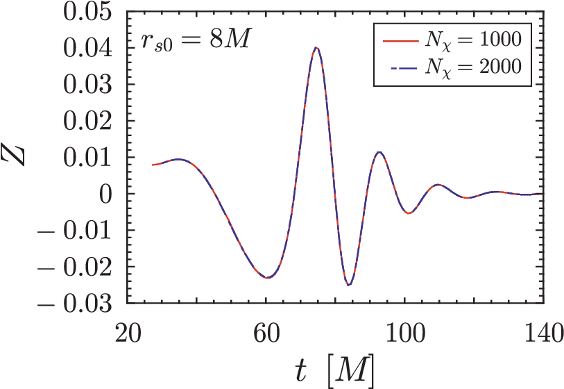
In order to verify our numerical code, we have calculated quadrupole gravitational radiations emitted during the collapse of a nonmagnetized homogeneous dust sphere, i.e., the gravitational waves emitted from the Oppenheimer-Snyder solution. The number of spatial grid points inside the star, $N_{\chi}$ , which corresponds to region I, is chosen to be $N_{\chi}=1000$ , because we can not see a dramatic improvement with lager number of grid points. Actually, as shown in Fig. 2, the waveforms of gravitational waves emitted from the collapsing dust ball with $N_{\chi}=1000$ are very similar to those with $N_{\chi}=2000$ , and the total energies of emitted gravitational waves defined later also agree with each other within $0.626$ % for $r_{s0}=8M$ and $1.37$ % for $r_{s0}=20M$ . In region III, the step size for integration is given as $\Delta\tilde{u}=(u_{\rm max}-u_{0})/N_{\tilde{u}}$ , where $u_{\rm max}$ is determined with the expected maximum time for observer, $t_{\rm max}$ , and the position of observer described in tortoise coordinate, $r_{*{\rm ob}}$ , as $u_{\rm max}\equiv t_{\max}-r_{*{\rm ob}}$ . In this paper we adopt that $t_{\rm max}=2000M$ and $r_{\rm ob}=r_{s0}+40M$ , respectively, where the position of observer is the same choice as the previous study by Cunningham, Price & Moncrief [20]. Since the numerical code in this region is essentially the same as that in Paper I, the number of grid points for outgoing null coordinate, $\tilde{u}$ , in region III is assumed to be $N_{\tilde{u}}=10000$ in this paper (see Table I in Paper I for the convergence test). Then we have only one parameter to determine the emitted gravitational waves, i.e., the initial radius $r_{s0}$ .

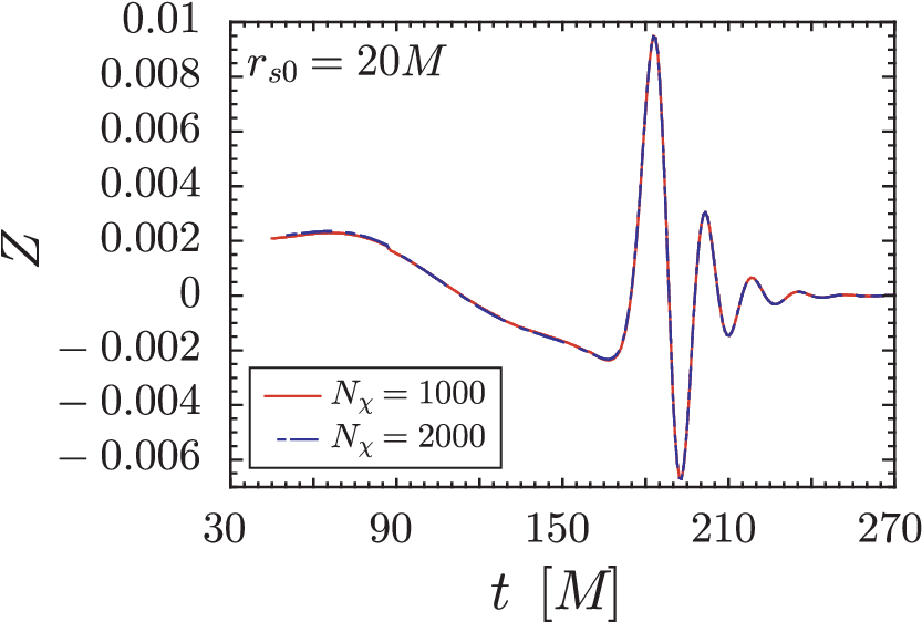As noticed in [20], the emitted gravitational waves are characterized by the quasi-normal ringing oscillation and subsequent power-law tail. In Fig. 3, we show the waveform of the gravitational waves for $l=2$ emitted during the collapse of the homogeneous dust ball, where the left and right panels are focused on the quasi-normal ringing and on the power-law tail, respectively. The fundamental frequency of the quasi-normal ringing have been calculated by Chandrasekhar & Detweiler [35], such as $2M\omega=0.74734+0.17792i$ . On the other hand, our numerical results show that the oscillation frequency is $2M\omega=0.737$ , which agrees well with the previous value with only $1.3\%$ error, while the damping rate also consorts with the theoretical value (see the left panel of Fig. 3). As for the late-time tail, in the right panel of Fig. 3, we find that the amplitude of gravitational wave decays as $(t-t_{0})^{-6}$ , where $t_{0}$ is the time when the observer receives the first signal emitted from the stellar surface, i.e., $t_{0}\equiv r_{*\rm ob}-r_{*s0}$ . This result is in good agreement with the analytical estimate by Price [36], that is $(t-t_{0})^{-(2l+2)}$ . Through these estimations for the frequency of quasi-ringing and the late-time tail, we believe that our numerical code is possible to derive the gravitational waves with high accuracy.

At the end in this section, we compare the total energy emitted during the collapse with the previous results by Cunningham, Price, & Moncrief [20] (CPM1979). It is worth to notice that the variables inside the star adopted in CPM1979 are different from those in the equation system for the gauge-invariant formalism proposed by Gerlach & Sengupta [22] and Gundlach & Martín-García [26]. The total emitted energy, $E_{\rm GW}$ , is estimated by integrating the luminosity of gravitational waves, $L_{\rm GW}$ , with respect to time, where the luminosity is defined as

L_{\rm GW}=\frac{1}{384\pi}\left({Z}_{,t}\right)^{2},

(92)

for the $l=2$ gravitational waves (e.g., [20]). In Fig. 4 we show the total emitted energy of gravitational waves as a function of the initial stellar radius $r_{s0}$ , where for comparison we also plot the result of CPM1979. It notes that in this figure we adopt the normalization for the quadrupole moment, $q_{2}$ , so that $q_{2}=2M$ as mentioned before. This figure shows that there are small difference between our results and those obtained in CPM1979. The main reason for this difference could be the difference how to choose the variables inside the star. Additionally as we noticed in Paper I, the difference of the accuracy in numerical code might be also added in the reason. Anyway we can observe that the total emitted energy systematically decreases as the initial stellar radius increases and that the emitted energy is very similar to that of CPM1979. Furthermore, with our variables inside the star and with our initial data, we derive the empirical formula for the total emitted energy as

\frac{E_{\rm GW}}{2M}=3.37\times 10^{-5}\times\left(\frac{r_{s0}}{2M}\right)^{-3},

(93)

which is also plotted in Fig. 4.

VI Gravitational Radiations from the OS solution

In order to calculate the gravitational waves emitted from the collapsing phase of a magnetized dust sphere, we have to provide the initial distribution of the magnetic field. In other words, one needs to set up the functional forms of $b_{2}$ and $b_{3}$ on the hypersurface $\eta=0$ . The initial distributions can be determined as the following two conditions are satisfied; (a) the regularity condition at the stellar center and (b) the junction condition at the stellar surface. Since we made assumptions in this paper that the magnetic field is confined inside the star and then the value of $q$ becomes zero at stellar surface, the conditions at the stellar surface can be described as $b_{1}(\chi_{0})=b_{2}(\chi_{0})=b_{3}(\chi_{0})=0$ . Now we introduce two new variables, $\bar{b}_{2}$ and $\bar{b}_{3}$ , such as

	$\displaystyle b_{2}(\chi)$	$\displaystyle={\cal B}_{2}\sin^{2}\chi\,\bar{b}_{2}(\chi),$		(94)
	$\displaystyle b_{3}(\chi)$	$\displaystyle={\cal B}_{3}\sin^{3}\chi\,\bar{b}_{3}(\chi),$		(95)

where ${\cal B}_{2}$ ${\cal B}_{3}$ are arbitrary constants related to the strength of the magnetic field. With analytic functions $\bar{b}_{2}$ and $\bar{b}_{3}$ , the regularity condition at the stellar center for the magnetic field is automatically satisfied. Since the geometry of the magnetic field when the collapse sets in is practically unknown, in this paper we adopt the following two types of the initial distributions for the magnetic field;

	$\displaystyle{\rm(I):}$	$\displaystyle\ \bar{b}_{2}(\chi)=\bar{b}_{3}(\chi)=1-2\left(\frac{\chi}{\chi_{0}}\right)^{2}+\left(\frac{\chi}{\chi_{0}}\right)^{4},$		(96)
	$\displaystyle{\rm(II):}$	$\displaystyle\ \bar{b}_{2}(\chi)=\bar{b}_{3}(\chi)=16\left(\frac{\chi}{\chi_{0}}\right)^{4}\left[1-2\left(\frac{\chi}{\chi_{0}}\right)^{2}+\left(\frac{\chi}{\chi_{0}}\right)^{4}\right],$		(97)

where the maximum value of $\bar{b}_{2}$ and $\bar{b}_{3}$ are chosen to be one in the range of $0\leq\chi\leq\chi_{0}$ . For the first profile (I) the magnetic field is stronger in the center of the sphere, while for the second profile (II) the field becomes stronger in the outer region. Additionally it notes that for both profiles the value of $b_{1}(\chi)$ , defined as $b_{1}(\chi)=-\partial_{\chi}b_{2}(\chi)/2$ , becomes zero at the stellar surface, i.e., as mentioned before the value of $q$ is zero at $\chi=\chi_{0}$ . With these magnetic profiles, we found that the allowed values for ${\cal B}_{2}$ and ${\cal B}_{3}$ have to be in a part of the range of ${\cal B}_{2}<{\cal B}_{3}$ , in order to produce the initial data set so that the inner metric perturbation should be smoothly connected to the stationary solution in the outer region at the stellar surface. So, in what follows, we consider the two cases for magnetic field; one is that only toroidal magnetic component exists, i.e., ${\cal B}_{2}=0$ , and second is that the poloidal magnetic component also exists as well as toroidal one, where those are satisfied the condition that ${\cal B}_{2}<{\cal B}_{3}$ .

VI.1 Toroidal Magnetic Field

First we consider the case that only toroidal magnetic component exists, i.e., ${\cal B}_{2}=0$ . In this case, the source term in the equation (89) to determine the initial distribution, $\bar{\zeta}$ , is proportional to ${{\cal B}_{3}}^{2}$ . The value of ${\cal B}_{3}$ is determined so that the initial inner metric perturbation should be smoothly connected at the stellar surface to the stationary solution for exterior region. Then we can get the distributions for the initial inner metric perturbation, $\bar{\zeta}(\chi)$ , and for the initial density perturbation, $\omega(\chi)$ , which are shown in Fig. 5 with the two different magnetic profiles (I) and (II). In this figure the initial stellar radius is set to be $r_{s0}=8M$ , but the functional forms of $\bar{\zeta}(\chi)$ and $\omega(\chi)$ with the different initial stellar radii are very similar to that with $r_{s0}=8M$ . From this figure, we can see that the initial distributions of $\bar{\zeta}$ and $\omega$ depend strongly on the magnetic profiles even if the initial metric perturbations for exterior region are adopted the same as the stationary solution with $q_{2}=2M$ .

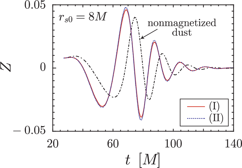
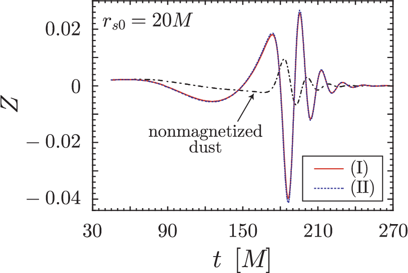
On the other hand, Fig. 6 shows the waveforms of the emitted gravitational waves with these initial perturbations, where the left and right panels are corresponding to the results with the initial radius $r_{s0}=8M$ and $20M$ , respectively. For comparison, the waveforms for the non-magnetized dust collapse are also plotted. The first observation of Fig. 6 is that the waveforms of the emitted gravitational waves are almost independent from the magnetic profiles in spite of the difference of initial perturbations inside the star. That is, if the initial dust sphere consists only of the toroidal magnetic component, it might be difficult to distinguish the interior magnetic profile by using the direct detection of the waveform of the emitted gravitational waves. Additionally we can observe the difference between the waveforms of gravitational waves with the toroidal magnetic field and without magnetic field. With smaller initial radius, the shape of waveform is similar to that for the nonmagnetized case, still we can see the effect of the existence of magnetic field, i.e., the quasi normal ringing can be seen earlier and the amplitude is also enhanced a little due to the magnetic effect. While, with large initial radius, it is possible to watch the obvious influence of magnetic field on the waveform of emitted gravitational waves, where the amplitude of waveform grows large and the maximum value of gravitational wave becomes a negative. In other words, with large initial radius, the waveform before the quasi normal ringing would be observed can be changed remarkably. The reason for this could be thought that with large initial radius it takes longer time until the stellar surface reaches to the event horizon and then the inner magnetic field can affect on the metric perturbations with longer time.

In particular, the dependence of magnetic effect on the initial radius can be seen clearly in the total energy of emitted gravitational waves. Fig. 7 shows the total energy as a function of the initial stellar radius with the circles for magnetic profile (I) and with the triangles for magnetic profile (II), where for comparison the total energies for the nonmagnetized dust case are also shown with the squares. It is found from this figure that with large initial radius, due to the magnetic effect the total energy of emitted gravitational wave becomes much larger than that for the nonmagnetized dust collapse. Then the dependence of the total energy for the dust collapse with toroidal magnetic field on the initial stellar radius, is quite different from the empirical formula (93) for the nonmagnetized dust collapse.

VI.2 Poloidal and Toroidal Magnetic Fields

Next we consider the magnetic field, which consists of the poloidal and toroidal components. In this case we can introduce the new parameter, $\beta$ , defined as $\beta={\cal B}_{2}/{\cal B}_{3}$ , and if we choose the value of $\beta$ the initial inner metric perturbations are determined as those should be smoothly connected to the outer stationary solution. It notes that the case for $\beta=0$ corresponds to the dust model, which only toroidal magnetic component exists shown in the previous subsection. Table 1 shows the allowed maximum values of $\beta$ with different combinations of magnetic profiles for the poloidal and toroidal components and with different initial stellar radii. From this table, it can be seen that with large initial radius it becomes more difficult to produce a magnetized dust model with large value of $\beta$ , and that the maximum values of $\beta$ depends strongly on the inner magnetic profiles.

Table 1: Allowed maximum values of

\beta

with the different combinations of magnetic profiles for the poloidal and toroidal components and with different initial stellar radii. As mentioned before,

b_{2}

and

b_{3}

are associated with the poloidal and toroidal magnetic components, respectively.

profile
$b_{2}$	$b_{3}$	$6M$	$8M$	$12M$	$16M$	$20M$	$24M$
(I)	(I)	$0.073$	$0.054$	$0.035$	$0.026$	$0.021$	$0.017$
(I)	(II)	$0.26$	$0.20$	$0.13$	$0.10$	$0.080$	$0.067$
(II)	(I)	$0.020$	$0.014$	$0.0094$	$0.0070$	$0.0055$	$0.0046$
(II)	(II)	$0.072$	$0.053$	$0.035$	$0.026$	$0.021$	$0.017$

Similar to the collapse of magnetized dust with only toroidal component, the magnetic effects can be seen in the waveforms of gravitational waves a little. Fig. 8 shows waveforms for the collapse of magnetized dust with $r_{s0}=8M$ and with several values of $\beta$ , where the magnetic profile (I) is adopted for the poloidal and toroidal components. From this figure it is found that the emitted gravitational waves are basically characterized by the quasi-normal ringing as well as the case of nonmagnetized dust collapse. While, we can also see the specific magnetic effects in the waveforms, where as the value of $\beta$ becomes larger, the amplitude of gravitational waves is enhanced and its maximum value changes from a positive to a negative. These are similar features to the case of dust collapse with only toroidal component with large initial radius. In other words, with large value of magnetic ratio, even with small initial radius, we can see the magnetic effect in the waveform before the quasi-normal ringing would be observed. This tendency holds for the magnetized dust collapse with different magnetic profiles. As a result, with large value of magnetic ratio, the total energy of gravitational waves grows. The total energies for $r_{s0}=8M$ and $20M$ are plotted in Fig. 9 as a function of magnetic ratio, where the different lines are corresponding to the different combinations of magnetic profiles for the poloidal and toroidal components. In the explanatory notes of this figure, for example, “(I)–(II)” denotes that the magnetic profiles (I) and (II) are adopted for the magnetic variables, $b_{2}$ and $b_{3}$ , respectively. This figure tells us that the total energies emitted in gravitational waves from the magnetized dust collapse depend strongly on the magnetic ratio and the inner magnetic profiles. This sensitivity, as well as the change of waveforms due to the existence of magnetic fields, could be important to extract some information of inner magnetic profiles of progenitor from the direct observation of gravitational waves during the black hole formation after the stellar collapse.

VII Conclusion

In this article, with the gauge-invariant perturbation theory we have studied the dependence of the stellar magnetic fields on the polar gravitational waves during the collapse of a homogeneous dust sphere. It should be emphasized that this is first calculation of emitted polar gravitational waves on the dynamical background spacetime with the covariant gauge-invariant formalism on the spherically symmetric spacetime and the coordinate-independent matching conditions at stellar surface, which is devised by Gundlach and Martín-García [26]. So far, such calculations could not be done due to the difficulty to treat the boundary conditions at stellar surface. While, in order to solve this difficulty, we evolve not only Zerille function, $Z$ , but also metric perturbation, $\tilde{\zeta}$ , in the intermediate exterior region (region II) and the calculation of emitted gravitational waves is successful.

With this nemerical code, we consider the magnetic effects on the polar gravitational waves from the Oppenheimer-Snyder solution describing collapsing dust, where the magnetic fields are introduced as a second order perturbation term. Even if the initial magnetic perturbations are small, as the collapse proceeds they could get amplified and become significant because of the conservation of magnetic flux. In particular, similar to Paper I, we have assumed that the magnetic field is axisymmetric, where the dipole magnetic field perturbations are the ones that couple to the quadrupole polar perturbations of the gravitational field. Additionally, we assumed momentarily static initial data and we have not taken into account the influence of the exterior magnetic field in the propagating gravitational waves.

Through the investigation, it is found that there exists an evidence of the strong influence of the magnetic field in the gravitational wave luminosity during the collapse. Depending on the initial profile of the magnetic field and its ratio between the poloidal and toroidal components, the energy outcome can be easily up to a few order higher than what we get from the nonmagnetized collapse. In addition, it is possible to observe an important change before the quasi-normal ringing is detected, which is induced by the presence of the magnetic field. These magnetic effects can be seen the collapsing model with large inital radius and with large magnetic ratio between the poloidal and toroidal components, since for a large initial radius the time needed for the black hole formation is longer and then the magnetic field acts for longer time on the collapsing fluid. It notes that the magnetic effects on the polar gravitational waves are different from those on the axial ones, i.e., the axial gravitational waves are independent from the magnetic ratio while they depend only on the magnetic strenght such as the value of ${\cal B}_{2}\times{\cal B}_{3}$ . Such magnetic effects could be helpful to extract some information of inner magnetic profiles of progenitor form the detection of gravitational waves radiated from the black hole formation after the stellar collapse.

At the end, we believe that although this study might be considered as a “toy problem” it has most of the ingredients needed in emphasizing the importance of the magnetic fields in the study of the gravitational wave output during the collapse. The final answer to the questions raised here would be provided by the 3D numerical MHD codes (see in [18, 37] for the recent developments), but this work provides hints and raises issues that need to be studied. Furthermore, as future studies, we condiser to study magnetic effects on the gravitational waves emitted from the more complicated background collapsing models such as inhomogeneous dust collapse and the stellar collapse with perfect fluid, while it should be also important to take into account the background magnetic field such as [38].

Acknowledgements.

We would like to thank K.D. Kokkotas and J.M. Martín-García for valuable comments. This work was supported via the Transregio 7 “Gravitational Wave Astronomy” financed by the Deutsche Forschungsgemeinschaft DFG (German Research Foundation).

Appendix A Concrete Expression for the Source Terms

In this appendix, we show the concrete expression for the source terms in the perturbation equations, which are not written in the main text. Those for Eqs. (21) – (23) and (25) – (27) are

$\displaystyle S_{\zeta}=$	$\displaystyle 16\pi\left[T^{3}+2(n^{A}T_{A})^{\prime}-n^{A}n^{B}T_{AB}+2(2\nu-W)n^{A}T_{A}\right]+4(\mu-U)\dot{k}+3\mu\dot{\zeta}+(2W-5\nu)\zeta^{\prime}$
	$\displaystyle-2(\mu-U)\dot{q}+(8\nu-6W)q^{\prime}+2q^{\prime\prime}+2\left[2(\mu-U)W-2\mu\nu-\mu^{\prime}+\dot{\nu}+8\pi t^{AB}u_{A}n_{B}\right]\psi$
	$\displaystyle+2\left[2W^{\prime}-2\nu^{2}+\frac{2}{r^{2}}-16\pi Q+8\pi(t^{A}_{\ A}+t^{AB}p_{AB})\right](\zeta+k)+16\pi Q\zeta+\frac{(l-1)(l+2)}{r^{2}}\zeta$
	$\displaystyle-2\left[4W^{\prime}+4\nu W-2W^{2}-2\nu^{2}+\frac{l(l+1)+4}{2r^{2}}-16\pi Q+8\pi(t^{A}_{\ A}+t^{AB}p_{AB})\right]q,$	(98)
$\displaystyle S_{k}=$	$\displaystyle 8\pi\left[(-c_{s}^{2}u^{A}u^{B}+n^{A}n^{B})T_{AB}+4Wn^{A}T_{A}\right]$
	$\displaystyle+(c_{s}^{2}+1)U\dot{\zeta}+\left[4U+c_{s}^{2}(\mu+2U)\right]\dot{k}+(c_{s}^{2}-1)W\zeta^{\prime}-(\nu+2c_{s}^{2}W)k^{\prime}-2U\dot{q}+2Wq^{\prime}$
	$\displaystyle+\Bigg[c_{s}^{2}\left\{8\pi(t^{A}_{\ A}-t^{AB}p_{AB})+2U(2\mu+U)+\frac{l(l+1)}{r^{2}}\right\}-8\pi(t^{A}_{\ A}+t^{AB}p_{AB})+2\left(W^{2}-\frac{1}{r^{2}}\right)\Bigg](\zeta+k)$
	$\displaystyle-\frac{(l-1)(l+2)}{2r^{2}}(c_{s}^{2}+1)\zeta-\left[c_{s}^{2}\left\{8\pi(t^{A}_{\ A}-t^{AB}p_{AB})+2U(2\mu+U)\right\}-8\pi(t^{A}_{\ A}+t^{AB}p_{AB})+6W^{2}-\frac{l(l+1)+2}{r^{2}}\right]q$
	$\displaystyle+2\left[(c_{s}^{2}+1)U(\nu+W)+(c_{s}^{2}-1)\mu W-8\pi(c_{s}^{2}+1)t^{AB}u_{A}n_{B}\right]\psi,$	(99)
$\displaystyle S_{\psi}=$	$\displaystyle 2\nu(\zeta+k)+2\mu\psi+\zeta^{\prime}-2q^{\prime}+2(W-\nu)q-16\pi n^{A}T_{A},$	(100)

and

$\displaystyle C_{\gamma}=$	$\displaystyle-W\dot{\zeta}+U\zeta^{\prime}+(2U-\mu)k^{\prime}-2Uq^{\prime}+\left[\frac{l(l+1)+2}{2r^{2}}+U(2\mu+U)-W(2\nu+W)+8\pi t^{A}_{\ A}\right]\psi,$	(101)
$\displaystyle C_{\omega}=$	$\displaystyle U\dot{\zeta}+(\mu+2U)\dot{k}+W\zeta^{\prime}-2Wk^{\prime}$
	$\displaystyle+\left[8\pi(t^{A}_{\ A}-t^{AB}p_{AB})+2U(2\mu+U)+\frac{l(l+1)}{r^{2}}\right](\zeta+k)-\frac{(l-1)(l+2)}{2r^{2}}\zeta$
	$\displaystyle-\left[8\pi(t^{A}_{\ A}-t^{AB}p_{AB})+2U(2\mu+U)\right]q+2\left[\nu U+\mu W+UW-8\pi t^{AB}u_{A}n_{B}\right]\psi,$	(102)
$\displaystyle C_{\alpha}=$	$\displaystyle 2\mu(\zeta+k)+2\nu\psi+\dot{\zeta}+2\dot{k}-2q(\mu+U),$	(103)

where $q$ is given by Eq. (24), such as

q=\frac{{b_{1}}^{2}-{b_{3}}^{2}}{\sqrt{5\pi}R^{2}}.

(104)

Additionally, the source terms in the perturbation equations for the metric perturbations (69) – (71) are

$\displaystyle\bar{S}_{\zeta}$	$\displaystyle=2\partial_{\chi}^{2}q-\frac{6\cos\chi}{\sin\chi}\partial_{\chi}q+\frac{4\cos^{2}\chi-l(l+1)+4}{\sin^{2}\chi}q+\frac{2}{\sqrt{5\pi}R^{2}\sin^{2}\chi}\left[\frac{2{b_{2}}^{2}}{\sin^{2}\chi}+{b_{1}}^{2}+{b_{3}}^{2}+2\partial_{\chi}(b_{1}b_{2})-\frac{6\cos\chi}{\sin\chi}b_{1}b_{2}\right],$	(105)
$\displaystyle\bar{S}_{k}$	$\displaystyle=\frac{2\partial_{\eta}R}{R}\partial_{\eta}q-\frac{2\cos\chi}{\sin\chi}\partial_{\chi}q+\frac{6\cos^{2}\chi-l(l+1)-2}{\sin^{2}\chi}q+\frac{1}{\sqrt{5\pi}R^{2}\sin^{2}\chi}\left[\frac{{b_{2}}^{2}}{\sin^{2}\chi}+{b_{1}}^{2}+{b_{3}}^{2}-\frac{4\cos\chi}{\sin\chi}b_{1}b_{2}\right],$	(106)
$\displaystyle\bar{S}_{\psi}$	$\displaystyle=2\partial_{\chi}q-\frac{2\cos\chi}{\sin\chi}q+\frac{2b_{1}b_{2}}{\sqrt{5\pi}R^{2}\sin^{2}\chi}.$	(107)

Appendix B Matter Perturbations for interior region

The matter perturbations are given by using the variables for metric and magnetic perturbations, which are determined after calculation for evolution of metric perturbations. With Eqs. (25) – (27), those are

	$\displaystyle\gamma=\frac{1}{8\pi\rho R^{2}}\left[\partial_{\eta}\partial_{\chi}k-\frac{\cos\chi}{\sin\chi}\partial_{\eta}\zeta+\frac{\partial_{\eta}R}{R}\partial_{\chi}\zeta+\frac{\partial_{\eta}R}{R}\partial_{\chi}k-\frac{2\partial_{\eta}R}{R}\partial_{\chi}q+\left\{\frac{l(l+1)}{2\sin^{2}\chi}+3\left(\frac{\partial_{\eta}R}{R}\right)^{2}+1-4\pi\rho R^{2}\right\}\psi\right],$		(108)
	$\displaystyle\omega=\frac{1}{8\pi\rho R^{2}}\Bigg[-\partial_{\chi}^{2}k+\frac{2\partial_{\eta}R}{R}\partial_{\chi}\psi+\frac{\partial_{\eta}R}{R}\partial_{\eta}\zeta+\frac{3\partial_{\eta}R}{R}\partial_{\eta}k+\frac{\cos\chi}{\sin\chi}\partial_{\chi}\zeta-\frac{2\cos\chi}{\sin\chi}\partial_{\chi}k$
	$\displaystyle+\left\{6\left(\frac{\partial_{\eta}R}{R}\right)^{2}+\frac{l(l+1)}{\sin^{2}\chi}-8\pi\rho R^{2}\right\}(\zeta+k)-\frac{(l-1)(l+2)}{2\sin^{2}\chi}\zeta-6\left(\frac{\partial_{\eta}R}{R}\right)^{2}q$
	$\displaystyle+\frac{4\partial_{\eta}R}{R}\frac{\cos\chi}{\sin\chi}\psi+\frac{8\pi\kappa}{R^{2}\sin^{2}\chi}\left({b_{1}}^{2}+{b_{3}}^{2}-\frac{{b_{2}}^{2}}{\sin^{2}\chi}\right)\Bigg],$		(109)
	$\displaystyle\alpha=\frac{1}{16\pi\rho R}\left[\partial_{\chi}\psi+\frac{2\partial_{\eta}R}{R}(\zeta+k)+\partial_{\eta}\zeta+2\partial_{\eta}k-\frac{4\partial_{\eta}R}{R}q\right].$		(110)

References

[1] B.C. Barish, in Proceedings of the 17th International Conference on General Relativity and Gravitation, edited by P. Florides, B. Nolan, and A. Ottewill (World Scientific, New Jersey, 2005), p. 24.
[2] http://lisa.jpl.nasa.gov/
[3] S. Kawamura, et al., Class. Quant. Grav. 23, S125 (2006).
[4] N. Andersson and K.D. Kokkotas, Phys. Rev. Lett. 77, 4134 (1996).
[5] K.D. Kokkotas, T.A. Apostolatos, and N. Andersson, Mon. Not. R. Astron. Soc. 320, 307 (2001).
[6] H. Sotani, K. Tominaga, and K.I. Maeda, Phys. Rev. D 65, 024010 (2002).
[7] H. Sotani and T. Harada, Phys. Rev. D 68, 024019 (2003); H. Sotani, K. Kohri, and T. Harada, ibid 69, 084008 (2004).
[8] H. Sotani and K.D. Kokkotas, Phys. Rev. D 70, 084026 (2004); 71, 124038 (2005).
[9] H. Sotani, Phys. Rev. D 79, 064033 (2009).
[10] E. Gaertig and K.D. Kokkotas, Phys. Rev. D 78, 064063 (2008).
[11] W. Kastaun, Phys. Rev. D 74, 124024 (2006); 77, 124019 (2008).
[12] R.F. Stark and T. Piran, Phys. Rev. Lett. 55, 891 (1985).
[13] M. Shibata and S.L. Shapiro, Astrophys. J. Lett. 572, L39 (2002).
[14] L. Baiotti, et al., Phys. Rev. D 71, 024035 (2005).
[15] M.D. Duez, et al., Phys. Rev. Lett. 96, 031101 (2006).
[16] L. Baiotti and L. Rezzola, Phys. Rev. Lett. 97, 141101 (2006).
[17] H. Dimmelmeier, et al., Phys. Rev. Lett. 98, 251101 (2007).
[18] M. Anderson, et al., Phys. Rev. Lett. 100, 191101 (2008).
[19] J.R. Oppenheimer and H. Snyder, Phys. Rev. 56 455 (1939).
[20] C.T. Cunningham, R.H. Price, and V. Moncrief, Astrophys. J. 224, 643 (1978); 230, 870 (1979).
[21] E. Seidel and T. Moore, Phys. Rev. D 35, 2287 (1987); E. Seidel, E.S. Myra, and T. Moore, ibid 38, 2349 (1988); E. Seidel, ibid 42, 1884 (1990).
[22] U.H. Gerlach and U.K. Sengupta, Phys. Rev. D 19, 2268 (1979); 22, 1300 (1980).
[23] H. Iguchi, K. Nakao, and T. Harada, Phys. Rev. D 57, 7262 (1998); H. Iguchi, T. Harada, and K. Nakao, Prog. Theor. Phys. 101, 1235 (1999); 103, 53 (2000).
[24] G. Lemaître, Ann. Soc. Sci. Bruxelles A 53, 51 (1933); R.C. Tolman, Proc. Natl. Acad. Sci. U.S.A. 20, 169 (1934); H. Bondi, Mon. Not. R. Astron. Soc. 107, 410 (1947).
[25] T. Harada, H. Iguchi, and M. Shibata, Phys. Rev. D 68, 024002 (2003).
[26] C. Gundlach and J.M. Martín-García, Phys. Rev. D 61, 084024 (2000); J.M. Martín-García and C. Gundlach, ibid. 64, 024012 (2001).
[27] H. Sotani, S. Yoshida, and K.D. Kokkotas, Phys. Rev. D 75, 084015 (2007) (Paper I).
[28] H. Sotani, K.D. Kokkotas, and N.Stergioulas, Mon. Not. R. Astron Soc. 375, 261 (2007); 385, L5 (2008).
[29] H. Sotani, A. Colaiuda, and K.D. Kokkotas, Mon. Not. R. Astron Soc. 385, 2161 (2008).
[30] H. Sotani and K.D. Kokkotas, accepted in Mon. Not. R. Astron Soc., preprint (0902.1490 [astro-ph]).
[31] E. Nakar, A. Gal-Yam, T. Piran, and D.B. Fox, Astrophys. J. 640, 849 (2006).
[32] M. Shibata, M.D. Duez, Y.T. Liu, S.L. Shapiro, and B.C. Stephens; Phys. Rev. Lett. 96, 031102 (2006).
[33] J.M. Martín-García and C. Gundlach, Phys. Rev. D 59, 064031 (1999).
[34] R.S. Hamadé and J.M. Stewart, Class. Quantum Grav. 13, 497 (1996).
[35] S. Chandrasekhar and S. Detweiler, Proc. R. Soc. London A344, 441 (1975).
[36] R.H. Price, Phys. Rev. D 5, 2419 (1972).
[37] B. Giacomazzo, L. Rezzolla, and L. Baiotti, preprint (0901.2722 [gr-qc]).
[38] K.D. Kokkotas, H. Sotani, P. Laguna, and C. Sopuerta, in preparation.

		$\displaystyle 2v^{C}\left(k_{AB\|C}-k_{CA\|B}-k_{CB\|A}\right)-\left[\frac{l(l+1)}{r^{2}}+G_{C}^{\ C}+G_{a}^{\ a}+2{\cal R}\right]k_{AB}-2g_{AB}v^{C}\left(k_{ED\|C}-k_{CE\|D}-k_{CD\|E}\right)g^{ED}$
		$\displaystyle\hskip 56.9055pt+g_{AB}\left(2v^{C\|D}+4v^{C}v^{D}-G^{CD}\right)k_{CD}+g_{AB}\left[\frac{l(l+1)}{r^{2}}+\frac{1}{2}\left(G_{C}^{\ C}+G_{a}^{\ a}\right)+{\cal R}\right]k_{D}^{\ \ D}$
		$\displaystyle\hskip 56.9055pt+2\left(v_{A}k_{\|B}+v_{B}k_{\|A}+k_{\|A\|B}\right)-g_{AB}\left[2k_{\|C}^{\ \ \|C}+6v^{C}k_{\|C}-\frac{(l-1)(l+2)}{r^{2}}k\right]=-16\pi T_{AB},$		(14)
		$\displaystyle k_{\|A}-k_{AB}^{\ \ \ \|B}+k_{B\ \ \|A}^{\ \ B}-v_{A}k_{B}^{\ \ B}=-16\pi T_{A},$		(15)
		$\displaystyle\left(k_{\|A}^{\ \ \|A}+2v^{A}k_{\|A}+G_{a}^{\ a}k\right)-\left[k_{AB}^{\ \ \ \|A\|B}+2v^{A}k_{AB}^{\ \ \ \|B}+2\left(v^{A\|B}+v^{A}v^{B}\right)k_{AB}\right]$
		$\displaystyle\hskip 56.9055pt+\left[k_{A\ \ \|B}^{\ \ A\ \ \|B}+v^{A}k_{B\ \ \|A}^{\ \ B}+{\cal R}k_{A}^{\ \ A}-\frac{l(l+1)}{2r^{2}}k_{A}^{\ \ A}\right]=16\pi T^{3},$		(16)
		$\displaystyle k_{A}^{\ A}=-16\pi T^{2},$		(17)

Gravitational Radiation from Collapsing Magnetized Dust. II – Polar Parity Perturbation –