A Dispersive Analysis on the $f_{0}(600)$ and $f_{0}(980)$ Resonances in $\gamma\gamma\to\pi^{+}\pi^{-},\pi^{0}\pi^{0}$ Processes

In the coupled channel case the relation between (the 2 by 2) $S$ matrix and $T$ matrix is

where $\rho=diag(\rho_{1},\rho_{2})$ and $\rho_{n}=\sqrt{1-4m_{n}^{2}/s}$. Here subscripts $n=1,2$ represent $\pi\pi,\bar{K}K$ channels, respectively.

Let $F_{1},F_{2}$ be the $\gamma\gamma\longrightarrow\pi\pi,\bar{K}K$ amplitudes, respectively, $F\equiv(F_{1},F_{2})^{T}$. Define $F^{\pm}(s)=\lim_{\epsilon\rightarrow 0^{+}}F(s\pm i\epsilon)\ ,$ then $F$ obeys the following spectral representation in the physical region:

above $\bar{K}K$ threshold and

when $s$ lies between first and second threshold. From Eqs. (2), (3), along positive real axis, one has a shorthand expression,

where $\theta_{1}=\theta(s-4m_{\pi}^{2})$ and $\theta_{2}=\theta(s-4m_{K}^{2})$ are step functions.

From above spectral function representations, the analytic continuation of $F$ to different sheets can be obtained:

These expressions of analytic continuation will be used later when extracting the residue couplings of each resonance.

In this subsection we review the method originally proposed by Basdevant and collaborators [5] on how to set up the dispersive representation for the $\gamma\gamma\to\pi\pi$ amplitudes.

On the right hand cut, $F^{+}=\tilde{S}F^{-}$. Further let $\tilde{F}=F-F_{L}$, $F_{L}$ contains only left hand cut of $F$. In this paper we approximate $F_{L}$ by its Born term, $F_{B}$. Then on the positive real axis one has,

Next we will search for a $2\times 2$ invertible matrix function $D(s)$, which is analytic on the cut $s$ plane and only contains right hand cut ($r.h.c.$), and on the $r.h.c.$ it obeys the same unitarity equation as $F(s)$. That is

One can then deduce from the above equation and Eq. (8) that

from which one obtains a dispersive representation for $\tilde{F}^{+}$

where $P$ is a 2 dimensional array of subtraction polynomial, and a proper subtraction is understood on the dispersion integral. By making use of Low’s theorem [16] which tells that when $s\rightarrow 0$, $F(s)\rightarrow F_{B}(s)$, we can rewrite the above equation with one more subtraction, and obtain: [17]

From the above discussion we know that the $\gamma\gamma\rightarrow\pi\pi,\bar{K}K$ amplitudes can be fit with parameter(s) $P$, once $D(s)$ and $F_{B}(s)$ are known.

The 2 by 2 matrix function $D(s)$ only contains right hand cuts, and satisfies the similar unitarity relations as $F$:

The above two equations have the same structure as the following

Hence searching for solutions of $D(s)$ is equivalent to searching for two independent solutions of the equation for the two dimensional array $(\chi_{1},\chi_{2})^{T}$. The two independent solutions can be identified as $(D_{11},D_{21})^{T}$ and $(D_{12},D_{22})^{T}$. The integral equation to solve Eq. (15) is

where $N$ denotes the number of steps in the iteration, the integration is truncated at $\Lambda^{2}=2.4\mathrm{GeV}^{2}$. On the $r.h.s.$ of above equation, we take the real part of the numerator in the integrand which is of great help in increasing the speed of convergence. [18] In the numerical calculation a convergent solution emerges after approximately 15 steps of iteration.

In this paper we solve the coupled channel $D(s)$ function in the case of $I,J=0,0$, for a given $T$ matrix. For the two $d$ waves and the $I=2$ $s$ wave we only use single channel approximation, and in such simplified case the solution to the function $D(s)$ is known as the Omnés solution,

In order to extract pole residues on different sheets a knowledge of analytic continuation to the complex plane is needed. Firstly, the analytic continuation of function $D(s)$ is simple. It satisfies the following dispersive integral equation£º

$D(s),\rho(s),T(s),\theta$ in above can all be matrix functions in above formula. To calculate $D$ with complex argument $z$ on the first Riemann sheet one only needs to replace $s\rightarrow z$ in above integral formula. For function $F$ the analytic continuation is more involved, in the following we discuss this topic in some details.

Residues of second sheet poles:

Since in the vicinity of a pole $z_{II}$, $S(s\sim z_{II})\simeq S^{\prime}(z_{II})(s-z_{II})$ and

and through the definition of coupling constants:

one obtains the expressions of $g_{\pi}$ and $g_{\gamma}$ for second sheet poles:

Residues of third sheet poles:

Denote the third sheet pole as $z_{III}$, which is the zero of $\mathrm{det}\,S$, then

From

the residues are hence obtainable, according to Eq. (21):

From Eq. (5) one further gets

Having obtained the two photon couplings, $g_{\gamma}$, the width of $\sigma$, $f_{0}(980)$ and $f_{2}(1270)$ to two photons can be calculated,

where $\alpha=1/137$ is the fine structure constant and $\beta_{R}=(1-4m_{\pi}^{2}/m_{R}^{2})^{1/2}$.

For the $\gamma\gamma\rightarrow\pi\pi$ process there are two independent helicity amplitudes $M_{++}$, $M_{+-}$. The former corresponds to photon helicity difference $\lambda=0$ the latter corresponds to $\lambda=2$. They contribute to the differential cross-section as: [4]

where $\rho=[1-4m_{\pi}^{2}/s]^{1/2}$, and they have partial wave expansions involving only even $J(\geq\lambda)$,

With this normalization the total cross-section reads,

At very low energies the major contribution to the amplitudes comes from one $\pi$ exchange (OPE), i.e., the Born term, as guaranteed by Low’s theorem. [16]

Denoting $s$–channel partial wave of the Born amplitude as $B_{J\lambda}(s)$, then Low’s theorem implies

The OPE Born term amplitude for $\gamma\gamma\rightarrow\pi^{0}\pi^{0}$ vanishes and for $\gamma\gamma\rightarrow\pi^{+}\pi^{-}$ processes read,

from which OPE partial wave amplitudes are obtained: [4]

At higher energies, however, OPE Born term amplitudes are not satisfactory to describe the left cut well. One may try to improve this by adding crossed channel vector and axial vector meson exchange diagrams. Nevertheless it is difficult to judge to what extent adding vector and axial vector exchange contributions improve the situation. Further discussions will be made in section 5.1.

Only I,J=0,0 channel are calculated by solving coupled channel integral equations. Other channels are all approximated by Omnés solutions. Subtraction polynomial (constant) in different channels are listed below:

• •

  $I,J,\lambda=0,0,0$: Solve couple-channel integral equation for $D$ and fit parameters are $P_{1}$ and $P_{2}$.

• •

  $I,J,\lambda=2,0,0$: Use Omnés solution, the fit parameter is $P_{3}$.

• •

  $I,J,\lambda=0,2,2$: Use Omnés function and fit $P_{4}$.

• •

  $I,J,\lambda=2,2,2$: Since this channel’s contribution is very weak, we use Born term approximation.

• •

  $I,J,\lambda=0,2,0$: Use Omnés solution and the fit parameter is $P_{5}$.

• •

  $I,J,\lambda=2,2,0$: Since this channel’s contribution is very weak, we use Born term approximation.

Here five subtraction constants are involved. Furthermore we introduce two additional form-factors to suppress the bad high energy behavior of the Born term amplitudes:

hence totally we have 7 fit parameters.

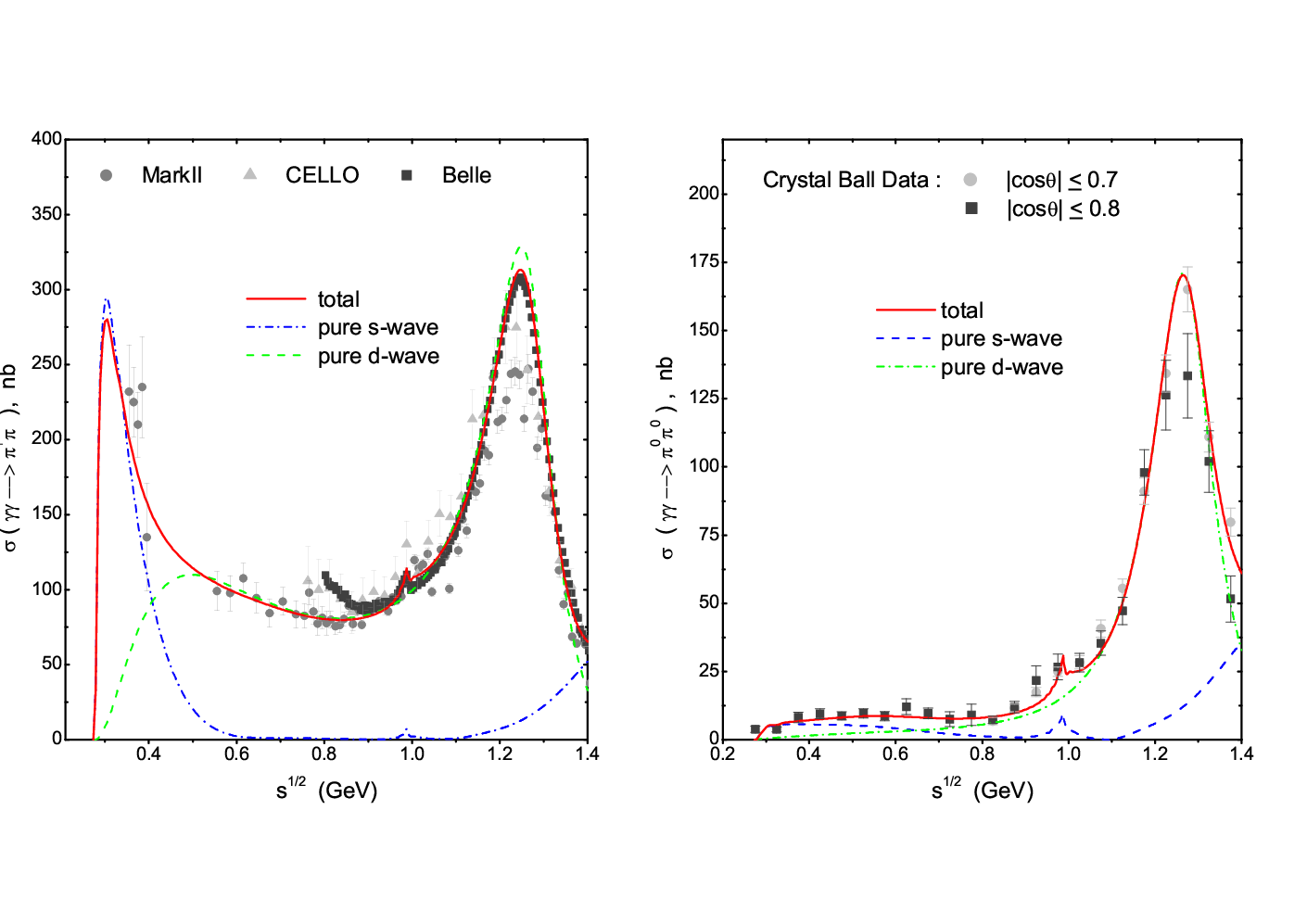
For $\gamma\gamma\rightarrow\pi^{+}\pi^{-}$ process there exist three sets of data, which are from Belle, [1] CELLO, [29] and Mark-II. [30] In our fit from $\pi^{+}\pi^{-}$ threshold to 0.9GeV, we use the Mark-II data, from 0.9GeV to 1.4GeV we use Belle data. For $\gamma\gamma\rightarrow\pi^{0}\pi^{0}$ there exist two data sets from Crystal Ball Collaboration, Refs. [31] and [32]. Here we chose the data from Ref. [31], from $\pi\pi$ threshold up to 1.4GeV.

Firstly a comparison between the contribution from OPE Born term amplitude and the contribution adding vector and axial vector meson exchanges in each channel is made, having obtained the two cutoff parameters which used to readjust the Born term amplitudes: $\Lambda_{s}=1.77$GeV and $\Lambda_{d}=0.86$GeV. However it is difficult to judge wether adding vector meson and axial vector meson exchange contributions improves the OPE contribution or not, comparing with the fit results shown in figure 3, where contributions from one $\pi$ exchange, vector meson exchange, axial-vector meson exchange, with corrections from the exponential form-factors (the latter are determined from the fit), are combined together and plotted. For the expressions of vector and axial vector meson exchange contributions we refer to the appendix.

The ratio between $IJ\lambda=020$ wave and $IJ\lambda=022$ wave may not be very stable. Though it is understood that the former should be much smaller than the latter. [33] We however find a convergent solution with $\sigma_{d0}/\sigma_{tot}\simeq 0.14$ and $\sigma_{s}/\sigma_{tot}\simeq 0.07$ (at the $f_{2}(1270)$ pole position). The first ratio given here is rather close to the ‘$dip$’ solution of Ref. [34]. The second ratio is significantly smaller than both the ‘$peak$’ and the ‘$dip$’ solution of Ref. [34]. The fit results are listed in table 4 and plotted in figure 4. The fit result on each partial wave amplitude is found to be rather similar in general with the solution B of Ref. [2] and to figure 1 of Ref. [9]. The di-photon width $\Gamma(f_{2}\to 2\gamma)=4.36$keV here, which is larger than the value given by the solution B of Ref. [2]: $\Gamma(f_{2}\to 2\gamma)=3.82\pm 0.30$keV. Part of the reason for such a difference may be due to the fact that the $s$-wave contribution given in this paper at the $f_{2}(1270)$ peak is smaller than that given in Ref. [2]. Also the interference between $s$ wave and $d$ wave is found to be destructive.³³ 3 Due to the limitation of experimental detection, the integration range of $\cos\theta$ is not from -1 to +1, hence causing a nonvanishing interference between different partial waves. That the result of Ref. [2] on $f_{2}(1270)$ di-photon width is significantly larger than the value as quoted by PDG is explained in Ref. [2] – because the Belle data gives a larger enhancement at $f_{2}(1270)$ peak than the previous data.

To summarize, we have the following observations through our fit:

1. 1.

   It is known that the $\lambda=2$ amplitude should dominate the $\gamma\gamma$ width of the tensor state. Even though the ratio between the $\lambda=0$ and the $\lambda=2$ partial wave may not be stable, a solution with a small ratio $\sigma_{d0}/\sigma_{tot}$ is found. The total di-photon decay width of $f_{2}(1270)$ is however found to be rather large comparing with the value quoted by PDG and the value given in Ref. [2].

2. 2.

   The $f_{0}(980)\to\gamma\gamma$ width is found to be very small. It is in agreement with the solution B in Ref. [2]. See table 6 for a comparison between different model predictions.

3. 3.

   We also give the $f^{\mathrm{III}}_{0}(980)$ width to two photons, which is not seen in previous literature. However the third sheet pole’s position and hence its residue are not quite stable, hence this number should be treated with care.

4. 4.

   The $\sigma$ width is smaller than most values given in the literature.

We have noticed that the low energy physics related to the $\sigma$ pole as described by the coupled channel $T$ matrix is not very satisfactory. Because the lack of crossing symmetry, occurrence of spurious poles, and the distortion of the $\sigma$ pole location. All these defects could affect a reliable extraction of the two photon coupling of the $\sigma$ meson. We try to remedy these defects by refitting the low energy data using a single channel $T$ matrix with all the nice properties such as analyticity, crossing symmetry, unitarity and with a reliable $\sigma$ pole location, since there is no coupled channel $T$ matrix with these properties available yet. The appropriate choice is the $\pi\pi$ scattering $T$ matrix proposed in Ref. [19], which gives the $\sigma$ pole location (The Eq. (21) of Ref. [19]):

and the residue:

to be compared with Eq. (44).⁴⁴ 4 The $g^{2}_{\sigma\pi\pi}$ coupling differs by a factor $16\pi$ from that of Ref. [10] where the $g_{\sigma\pi\pi}\simeq 3$GeV. Ref. [10] also quoted the number extracted from Ref. [35] in two ways, corresponding to $|g_{\sigma\pi\pi}|=3.4$ and 3.9GeV, respectively. Also the value in Eq. (47) is compatible with the result of Ref. [12, 36], $g^{2}_{\sigma\pi\pi}=-0.25-0.06i\mathrm{GeV}^{2}$.

We refit the $\gamma\gamma\to\pi^{+}\pi^{-},\pi^{0}\pi^{0}$ data below 800MeV using that $T^{I=0}_{J=0}$ and $T^{I=2}_{J=0}$ matrices and keeping $d$-waves fixed by the coupled channel fit described in section 5. That means contributions from all other partial waves are treated as background. In this situation we fit with only single parameter $P_{1}$, while keeping all other parameters fixed by the coupled channel fit. The result is given in table 5. We plot the fit curve in figure 5.

In this section we discuss the possibility that the two narrow width poles in the vicinity of $\bar{K}K$ threshold found in section 4 may be originated from a single Breit–Wigner parametrization.

For the $\pi\pi$, $\bar{K}K$ coupled channel system, one can make use of conformal mapping technique [37] to map the four sheets $s$ plane into the one sheet $\omega$ plane,

where $p_{i}=\frac{1}{2}\sqrt{s-4m_{i}^{2}}$ denotes the $i$-th channel momentum, $\Delta=\sqrt{m_{2}^{2}-m_{1}^{2}}$. The $\omega$-plane is depicted in figure 6:

In figure 6 $\omega=i,1$ corresponds to $s=4m_{\pi}^{2}$, $4m_{K}^{2}$, respectively. $S$ matrix elements can be written as,

References

• [1] T.ย Mori et al. (Belle Collaboration), Phys. Rev. D75(2007)051101.
• [2] M.ย R.ย Pennington, T.ย Mori, S.ย Uehara, Y.ย Watanabe, Eur. Phys. J.C56(2008)1.
• [3] M.ย R.ย Pennington, invited talk at YKIS Seminar on New Frontiers in QCD: Exotic Hadrons and Hadronic Matter, Kyoto, Japan, 20 Nov - 8 Dec 2006. Prog. Theor. Phys. Suppl. 168(2007)143.
• [4] D.ย Morgan, M.ย R.ย Pennington, Z.ย Phys. C48(1990)623; D.ย Morgan, M.ย R.ย Pennington, Z.ย Phys. C37(1988)431.
• [5] O.ย Babelon et al., Nucl. Phys. B113(1976)445; O.ย Babelon et al., Nucl. Phys. B114(1976)252.
• [6] G.ย Mennessier, Z.ย Phys. C16(1983)241.
• [7] A.ย V.ย Anisovich, V.ย V.ย Anisovich, Phys. Lett. B467(1999)289.
• [8] L.ย V.ย Filโ€™kov, V.ย L.ย Kashevarov, Phys. Rev. C72(2005)035211.
• [9] N.ย N.ย Achasov, G.ย N.ย Shestakov, arXive:0712.0885 [hep-ph].
• [10] J.ย A.ย Oller, L.ย Roca, C.ย Schat, Phys. Lett. B659(2008)201.
• [11] J.ย Bernabeu, J.ย Prades, Phys. Rev. Lett. 100(2008)241804.
• [12] G.ย Mennessier, S.ย Narison, W.ย Ochs, Phys. Lett. B665(2008)205.
• [13] K.ย L.ย Au, D.ย Morgan and M.ย R.ย Pennington, Phys. Rev. D35(1987)1633.
• [14] S.ย Pislak et al., Phys. Rev. D67(2003)072004.
• [15] J.ย R.ย Batley et al (The NA48/2 Collaboration), Euro. Phys. J. C54(2008)411.
• [16] F.ย E.ย Low Phys. Rev. 96(1954)1428; M.ย Gell-Mann, M.ย L.ย Goldberger, Phys. Rev. 96(1954)1433; H.ย D.ย I.ย Abarbanel, M.ย L.ย Goldberger, Phys. Rev. 165(1968)1594.
• [17] J.ย F.ย Donoghue and Barry R. Holstein, Phys. Rev. D48(1993)137; D. Morgan and M. R. Pennington, Phys. Lett. B272(1991)134
• [18] J.ย F. Donoghue, J.ย Gasser, H.ย Leutwyler, Nucl. Phys. B343(1990)341.
• [19] Z.ย Y.ย Zhou et al., JHEP 0502(2005)043.
• [20] J.ย J.ย Wang, Z.ย Y.ย Zhou, H.ย Q.ย Zheng, JHEP 0512(2005)019.
• [21] W.ย Ochs, Ph.D. thesis, Munich Univ., 1974.
• [22] D.ย H.ย Cohen et al., Phys. Rev. D22(1980)2595.
• [23] A.ย Etkin et al., Phys. Rev. D25(1982)1786 .
• [24] A. D. Martin, E. N. Ozmutlu, Nucl. Phys. B158(1979)520.
• [25] G.ย Costa et al., Nucl. Phys. B175(1980)402.
• [26] V.ย A.ย Polychronakos et al., Phys.ย Rev. D19(1979)1317.
• [27] M.ย P.ย Locher, V.ย E.ย Markushin, H.ย Q.ย Zheng, Eur.ย Phys.ย J. C4(1998)317.
• [28] D.ย Morgan, Nucl.ย Phys. A543(1992)632.
• [29] H.ย J.ย Behrend et al. (CELLO Collaboration), Z.ย Phys. C56(1992)381.
• [30] J.ย Boyer et al. (Mark-II Collaboration), Phys.ย Rev. D42(1990)1350.
• [31] H.ย Marsiske et al.(Crystal Ball Collaboration) Phys. Rev. D41(1990)3324.
• [32] J.ย K.ย Bienlein et al, Iโ€‹XIX Iโ€‹nโ€‹tโ€‹eโ€‹rโ€‹nโ€‹aโ€‹tโ€‹iโ€‹oโ€‹nโ€‹aโ€‹lInternational Wโ€‹oโ€‹rโ€‹kโ€‹sโ€‹hโ€‹oโ€‹pWorkshop oโ€‹non Pโ€‹hโ€‹oโ€‹tโ€‹oโ€‹nPhoton-Pโ€‹hโ€‹oโ€‹tโ€‹oโ€‹nPhoton Cโ€‹oโ€‹lโ€‹lโ€‹iโ€‹sโ€‹iโ€‹oโ€‹nโ€‹sCollisions, San. Diego, 1992, ed. D. Caldwell and H. P. Parr (World Scientific, 1992) p.241.
• [33] F.ย E.ย Close, Z.ย P.ย Li and T.ย Barnes, Phys.ย Rev. D43(1991)2161.
• [34] M.ย Boglione, M.ย R.ย Pennington, Eur.ย Phys.ย J. C9(1999)11.
• [35] I.ย Caprini, G.ย Colangelo, H.ย Leutwyler, Phys. Rev. Lett. 96, 132001 (2006).
• [36] R.ย Kaminski G.ย Mennesier, S.ย Narison, to appear.
• [37] M.ย Kato, Ann. Phys.31(1965)130.
• [38] Y.ย Fujii, M.ย Kato,Nuovo Cimento 13A(1973)311.
• [39] B.ย S.ย Zou, D.ย Bugg, Phys. Rev. D48(1993)3948.
• [40] Z.ย Y.ย Zhou, H.ย Q.ย Zheng, Nucl. Phys.A775(2006)212; H.ย Q.ย Zheng et al., Nucl. Phys. A733(2004)235;
• [41] J.ย Babcock, J.ย L.ย Rosner, Phys. Rev. D14(1976)1286.
• [42] T.ย Barnes, Phys. Lett. B165(1985)434.
• [43] S.ย Narison, Phys. Rev. D73(2006)114024; S. Narison, G. Veneziano, Int. J. Mod. Phys. A4(1989)2751; S.ย Narison, Nucl. Phys. B509(1998)312.
• [44] N.ย N.ย Achasov et al., Z.ย Phys. C16(1982)55.
• [45] T.ย Barnes, Proc. IXth Int. Workshop on Photon-Photon Collisions (San Diego, 1992), ed. D.ย Caldwell and H.ย P.ย Paar(World Scientific, 1992.), p.263
• [46] C.ย Hanhart, Yu.ย S.ย Kalashnikova, A.ย E.ย Kudryavtsev, A.ย V.ย Nefediev, Phys. Rev. D75(2007)074015.
• [47] C.ย Amsler et al. (Particle Data Group), Phys. Lett. B667(2008)1.
• [48] M.ย R.ย Pennington, Mod. Phys. Lett. A22(2007)1439.
• [49] F.ย Giacosa, T.ย Gutsche, V.ย Lyubovitskij, Phys. Rev. D77(2008)034007.
• [50] H.ย Q.ย Zheng, Plenary talk given at Workshop on Chiral Symmetry in Hadron and Nuclear Physics: Chiral07, Osaka, Japan, 13-16 Nov 2007; Mod. Phys. Lett. A23(2008)2218.
• [51] Z.ย H.ย Guo, L.ย Y.ย Xiao, H.ย Q.ย Zheng, Int. J. Mod. Phys. A22(2007)4603; M.ย X.ย Su, L.ย Y. Xiao, H.ย Q.ย Zheng, Nucl. Phys. A792(2007)288.
• [52] J.ย Gasser, S.ย Bellucci, M.ย E.ย Sainio, Nucl. Phys. B423(1994)80.
• [53] M.ย Suzuki, Phys. Rev. D47(1993)1252.
• [54] H.ย Y.ย Cheng, Phys. Rev. D67(2003)094007.
• [55] Z.ย H.ย Guo, Phys. Rev. D 78(2008)033004.
8 Appendix
In this section we describe the method how we calculate various vector meson and axial vector meson exchange contributions to the Born term amplitude. We use Proca field to describe spin 1 fields. For the 1โˆ’โฃโˆ’1^{--} vector meson, the interaction lagrangian is
โ„’kโ€‹iโ€‹n=โˆ’14<Vฮผโ€‹ฮฝโ€‹Vฮผโ€‹ฮฝโˆ’2โ€‹MV2โ€‹Vฮผโ€‹Vฮผ>.\mathcal{L}_{kin}=-\frac{1}{4}<V_{\mu\nu}V^{\mu\nu}-2M_{V}^{2}V^{\mu}V_{\mu}>. (60)
Proca field is also suitable to describe the two types of axial vector meson contributions: Aฮผยฏโ€‹(JPโ€‹C=1+โฃ+)\overline{A_{\mu}}(J^{PC}=1^{++}) and Bฮผยฏโ€‹(JPโ€‹C=1+โฃโˆ’)\overline{B_{\mu}}(J^{PC}=1^{+-}).
For ฯ€โ€‹ฯ€โ€‹ฮณ\pi\pi\gamma vertices, the lowest order ฯ‡โ€‹Pโ€‹T\chi PT amplitudes are calculable using the following interaction lagrangian:ย [52]
โ„’2ฯ‡โ€‹Pโ€‹T\displaystyle\mathcal{L}_{2}^{\chi PT} =\displaystyle= F24<uฮผโ€‹uฮผ>,\displaystyle\frac{F^{2}}{4}<u^{\mu}u_{\mu}>,
โ„’iโ€‹nโ€‹tโ€‹(V)\displaystyle\mathcal{L}_{int}(V) =\displaystyle= eโ€‹CVโ€‹ฮตฮผโ€‹ฮฝโ€‹ฯโ€‹ฯƒโ€‹Fฮผโ€‹ฮฝ<Vฯโ€‹{Q,uฯƒ}>,\displaystyle eC_{V}\varepsilon_{\mu\nu\rho\sigma}F^{\mu\nu}<V_{\rho}\{Q,u^{\sigma}\}>,
โ„’iโ€‹nโ€‹tโ€‹(Bยฏ)\displaystyle\mathcal{L}_{int}(\overline{B}) =\displaystyle= eโ€‹CBโ€‹Fฮผโ€‹ฮฝ<Bยฏฮผโ€‹{Q,uฮฝ}>,\displaystyle eC_{B}F^{\mu\nu}<\overline{B}_{\mu}\{Q,u^{\nu}\}>,
โ„’iโ€‹nโ€‹tโ€‹(Aยฏ)\displaystyle\mathcal{L}_{int}(\overline{A}) =\displaystyle= eโ€‹CAโ€‹Fฮผโ€‹ฮฝ<Aยฏฮผโ€‹[Q,uฮฝ]>,\displaystyle eC_{A}F^{\mu\nu}<\overline{A}_{\mu}[Q,u^{\nu}]>, (61)
where
Vฮผ\displaystyle V_{\mu} =\displaystyle= (ฯ02+ฯ‰2ฯ+Kโˆ—โฃ+ฯโˆ’โˆ’ฯ02+ฯ‰2Kโˆ—0Kโˆ—โฃโˆ’Kโˆ—ยฏโ€‹0โˆ’ฯ•)ฮผ,\displaystyle\left(\begin{array}[]{ccc}\frac{\rho_{0}}{\sqrt{2}}+\frac{\omega}{\sqrt{2}}&\rho^{+}&K^{*+}\\ \rho^{-}&-\frac{\rho_{0}}{\sqrt{2}}+\frac{\omega}{\sqrt{2}}&K^{*0}\\ K^{*-}&K^{\overline{*}0}&-\phi\end{array}\right)_{\mu},
Aยฏฮผ\displaystyle\overline{A}_{\mu} =\displaystyle= (a102+f1โ€‹(1285)2a1+K1โ€‹A+a1โˆ’โˆ’a102+f1โ€‹(1285)2K1โ€‹A0K1โ€‹Aโˆ’K1โ€‹A0ยฏf1โ€‹(1420))ฮผ,\displaystyle\left(\begin{array}[]{ccc}\frac{a_{1}^{0}}{\sqrt{2}}+\frac{f_{1}(1285)}{\sqrt{2}}&a_{1}^{+}&K_{1A}^{+}\\ a_{1}^{-}&-\frac{a_{1}^{0}}{\sqrt{2}}+\frac{f_{1}(1285)}{\sqrt{2}}&K_{1A}^{0}\\ K_{1A}^{-}&K_{1A}^{\overline{0}}&f_{1}(1420)\end{array}\right)_{\mu},
Bยฏฮผ\displaystyle\overline{B}_{\mu} =\displaystyle= (b102+h1โ€‹(1170)2b1+K1โ€‹B+b1โˆ’โˆ’b102+h1โ€‹(1170)2K1โ€‹B0K1โ€‹Bโˆ’K1โ€‹B0ยฏh1โ€‹(1380))ฮผ.\displaystyle\left(\begin{array}[]{ccc}\frac{b_{1}^{0}}{\sqrt{2}}+\frac{h_{1}(1170)}{\sqrt{2}}&b_{1}^{+}&K_{1B}^{+}\\ b_{1}^{-}&-\frac{b_{1}^{0}}{\sqrt{2}}+\frac{h_{1}(1170)}{\sqrt{2}}&K_{1B}^{0}\\ K_{1B}^{-}&K_{1B}^{\overline{0}}&h_{1}(1380)\end{array}\right)_{\mu}.
The K1โ€‹AK_{1A} and K1โ€‹BK_{1B} mesons are mixed states,
K1โ€‹A\displaystyle K_{1A} =\displaystyle= sinโกฮธโ€‹K1โ€‹(1270)+cosโกฮธโ€‹K1โ€‹(1400),\displaystyle\sin\theta K_{1}(1270)+\cos\theta K_{1}(1400),
K1โ€‹B\displaystyle K_{1B} =\displaystyle= โˆ’sinโกฮธโ€‹K1โ€‹(1400)+cosโกฮธโ€‹K1โ€‹(1270).\displaystyle-\sin\theta K_{1}(1400)+\cos\theta K_{1}(1270). (74)
The mixing angle |ฮธ|=37โˆ˜|\theta|=37^{\circ} or 58โˆ˜58^{\circ}[53, 54, 55]. Comparing with Ref.ย [52], we also introduced Aยฏฮผโ€‹(1+โฃ+)\overline{A}_{\mu}(1^{++}) exchanges here except the 1โˆ’โฃโˆ’,1+โฃโˆ’1^{--},1^{+-} contributions. Coefficients CV,CA,CBC_{V},C_{A},C_{B} are determined through ฯโก(770)โ†’ฯ€โ€‹ฮณ\rho(770)\rightarrow\pi\gamma, a1โ€‹(1260)โ†’ฯ€โ€‹ฮณa_{1}(1260)\rightarrow\pi\gamma and b1โ€‹(1235)โ†’ฯ€โ€‹ฮณb_{1}(1235)\rightarrow\pi\gamma processes.
Invariant amplitudes A,BA,B are obtainable using the above interaction lagrangian:
โˆ™ฮณโ€‹ฮณโ†’ฯ€0โ€‹ฯ€0:ฯ0,ฯ‰,b10,h1โ€‹(1170)\bullet\gamma\gamma\rightarrow\pi^{0}\pi^{0}:\rho_{0},\omega,b_{1}^{0},h_{1}(1170) contributes here.
AN,ฯt\displaystyle A_{N,\rho}^{t} =\displaystyle= CV29โ€‹F2โ€‹sโˆ’4โ€‹tโˆ’4โ€‹mฯ€2Mฯ2โˆ’t,\displaystyle\frac{C_{V}^{2}}{9F^{2}}\frac{s-4t-4m_{\pi}^{2}}{M_{\rho}^{2}-t},
BN,ฯt\displaystyle B_{N,\rho}^{t} =\displaystyle= CV218โ€‹F2โ€‹1Mฯ2โˆ’t,\displaystyle\frac{C_{V}^{2}}{18F^{2}}\frac{1}{M_{\rho}^{2}-t},
AN,ฯ‰t\displaystyle A_{N,\omega}^{t} =\displaystyle= CV2F2โ€‹sโˆ’4โ€‹tโˆ’4โ€‹mฯ€2Mฯ‰2โˆ’t=9โ€‹AN,ฯtโ€‹(Mฯโ†’Mฯ‰),\displaystyle\frac{C_{V}^{2}}{F^{2}}\frac{s-4t-4m_{\pi}^{2}}{M_{\omega}^{2}-t}=9A_{N,\rho}^{t}(M_{\rho}\rightarrow M_{\omega}),
BN,ฯ‰t\displaystyle B_{N,\omega}^{t} =\displaystyle= CV22โ€‹F2โ€‹1Mฯ‰2โˆ’t=9โ€‹BN,ฯtโ€‹(Mฯโ†’Mฯ‰),\displaystyle\frac{C_{V}^{2}}{2F^{2}}\frac{1}{M_{\omega}^{2}-t}=9B_{N,\rho}^{t}(M_{\rho}\rightarrow M_{\omega}),
AN,b1t\displaystyle A_{N,b_{1}}^{t} =\displaystyle= CB236โ€‹F2โ€‹s+4โ€‹tโˆ’4โ€‹mฯ€2Mb12โˆ’t,\displaystyle\frac{C_{B}^{2}}{36F^{2}}\frac{s+4t-4m_{\pi}^{2}}{M_{b_{1}}^{2}-t},
BN,b1t\displaystyle B_{N,b_{1}}^{t} =\displaystyle= CB272โ€‹F2โ€‹1Mb12โˆ’t,\displaystyle\frac{C_{B}^{2}}{72F^{2}}\frac{1}{M_{b_{1}}^{2}-t},
AN,h1t\displaystyle A_{N,h_{1}}^{t} =\displaystyle= CB24โ€‹F2โ€‹s+4โ€‹tโˆ’4โ€‹mฯ€2Mb12โˆ’t=9โ€‹AN,b1tโ€‹(Mb1โ†’Mh1โ€‹(1170)),\displaystyle\frac{C_{B}^{2}}{4F^{2}}\frac{s+4t-4m_{\pi}^{2}}{M_{b_{1}}^{2}-t}=9A_{N,b_{1}}^{t}(M_{b_{1}}\rightarrow M_{h_{1}(1170)}),
BN,h1t\displaystyle B_{N,h_{1}}^{t} =\displaystyle= CB28โ€‹F2โ€‹1Mb12โˆ’t=9โ€‹BN,b1tโ€‹(Mb1โ†’Mh1โ€‹(1170)),\displaystyle\frac{C_{B}^{2}}{8F^{2}}\frac{1}{M_{b_{1}}^{2}-t}=9B_{N,b_{1}}^{t}(M_{b_{1}}\rightarrow M_{h_{1}(1170)}), (75)
To get uu channel contributions we only need to replace tt by uu in above expressions, i.e. AN,iu=AN,itโ€‹(tโ†’u),BN,iu=BN,itโ€‹(tโ†’u)A_{N,i}^{u}=A_{N,i}^{t}(t\rightarrow u),\ B_{N,i}^{u}=B_{N,i}^{t}(t\rightarrow u)ยกยฃ
โˆ™ฮณโ€‹ฮณโ†’ฯ€+โ€‹ฯ€โˆ’:ฯ€,ฯ,b1,a1\bullet\gamma\gamma\rightarrow\pi^{+}\pi^{-}:\pi,\rho,b_{1},a_{1} contribute here.
AC,ฯ€Cโ€‹oโ€‹nโ€‹tโ€‹aโ€‹cโ€‹t\displaystyle A_{C,\pi}^{Contact} =\displaystyle= 4s,\displaystyle\frac{4}{s},
BC,ฯ€Cโ€‹oโ€‹nโ€‹tโ€‹aโ€‹cโ€‹t\displaystyle B_{C,\pi}^{Contact} =\displaystyle= 0,\displaystyle 0,
AC,ฯ€t\displaystyle A_{C,\pi}^{t} =\displaystyle= (2โ€‹t+sโˆ’2โ€‹mฯ€2)2s2โ€‹1(mฯ€2โˆ’t),\displaystyle\frac{(2t+s-2m_{\pi}^{2})^{2}}{s^{2}}\frac{1}{(m_{\pi}^{2}-t)},
BC,ฯ€t\displaystyle B_{C,\pi}^{t} =\displaystyle= 1mฯ€2โˆ’t,\displaystyle\frac{1}{m_{\pi}^{2}-t},
AC,ฯt\displaystyle A_{C,\rho}^{t} =\displaystyle= CV29โ€‹F2โ€‹sโˆ’4โ€‹tโˆ’4โ€‹mฯ€2Mฯ2โˆ’t=AN,ฯt,\displaystyle\frac{C_{V}^{2}}{9F^{2}}\frac{s-4t-4m_{\pi}^{2}}{M_{\rho}^{2}-t}=A_{N,\rho}^{t},
BC,ฯt\displaystyle B_{C,\rho}^{t} =\displaystyle= CV218โ€‹F2โ€‹1Mฯ2โˆ’t=BN,ฯt,\displaystyle\frac{C_{V}^{2}}{18F^{2}}\frac{1}{M_{\rho}^{2}-t}=B_{N,\rho}^{t},
AC,b1t\displaystyle A_{C,b_{1}}^{t} =\displaystyle= CB236โ€‹F2โ€‹s+4โ€‹tโˆ’4โ€‹mฯ€2Mb12โˆ’t=AN,b1t,\displaystyle\frac{C_{B}^{2}}{36F^{2}}\frac{s+4t-4m_{\pi}^{2}}{M_{b_{1}}^{2}-t}=A_{N,b_{1}}^{t},
BC,b1t\displaystyle B_{C,b_{1}}^{t} =\displaystyle= CB272โ€‹F2โ€‹1Mb12โˆ’t=BN,b1t,\displaystyle\frac{C_{B}^{2}}{72F^{2}}\frac{1}{M_{b_{1}}^{2}-t}=B_{N,b_{1}}^{t},
AC,a1t\displaystyle A_{C,a_{1}}^{t} =\displaystyle= โˆ’CA24โ€‹F2s+4โ€‹tโˆ’4โ€‹mฯ€2Ma12โˆ’t=โˆ’9AN,b1t(CBโ†’CA,Mb1โ†’Ma1),\displaystyle-\frac{C_{A}^{2}}{4F^{2}}\frac{s+4t-4m_{\pi}^{2}}{M_{a_{1}}^{2}-t}=-9A_{N,b_{1}}^{t}(C_{B}\rightarrow C_{A},M_{b_{1}}\rightarrow M_{a_{1}}),
BC,a1t\displaystyle B_{C,a_{1}}^{t} =\displaystyle= โˆ’CA28โ€‹F21Ma12โˆ’t=โˆ’9BN,b1t(CBโ†’CA,Mb1โ†’Ma1),\displaystyle-\frac{C_{A}^{2}}{8F^{2}}\frac{1}{M_{a_{1}}^{2}-t}=-9B_{N,b_{1}}^{t}(C_{B}\rightarrow C_{A},M_{b_{1}}\rightarrow M_{a_{1}}), (76)
To get uu channel contribution we only need to replace tt by uu in above expressions, i.e. AC,iu=AC,itโ€‹(tโ†’u),BC,iu=BC,iuโ€‹(tโ†’u)A_{C,i}^{u}=A_{C,i}^{t}(t\rightarrow u),\ B_{C,i}^{u}=B_{C,i}^{u}(t\rightarrow u)ยกยฃ
โˆ™ฮณโ€‹ฮณโ†’K+โ€‹Kโˆ’:K,Kโˆ—,K1โ€‹B,K1โ€‹A\bullet\gamma\gamma\rightarrow K^{+}K^{-}:K,K^{*},K_{1B},K_{1A} contribute.
AC,KCโ€‹oโ€‹nโ€‹tโ€‹aโ€‹cโ€‹t\displaystyle A_{C,K}^{Contact} =\displaystyle= 4s,\displaystyle\frac{4}{s},
BC,KCโ€‹oโ€‹nโ€‹tโ€‹aโ€‹cโ€‹t\displaystyle B_{C,K}^{Contact} =\displaystyle= 0,\displaystyle 0,
AC,Kt\displaystyle A_{C,K}^{t} =\displaystyle= (2โ€‹t+sโˆ’2โ€‹mK2)2s2โ€‹1(mK2โˆ’t)=AC,ฯ€tโ€‹(mฯ€โ†’mK),\displaystyle\frac{(2t+s-2m_{K}^{2})^{2}}{s^{2}}\frac{1}{(m_{K}^{2}-t)}=A_{C,\pi}^{t}(m_{\pi}\rightarrow m_{K}),
BC,Kt\displaystyle B_{C,K}^{t} =\displaystyle= 1mK2โˆ’t=BC,ฯ€tโ€‹(mฯ€โ†’mK),\displaystyle\frac{1}{m_{K}^{2}-t}=B_{C,\pi}^{t}(m_{\pi}\rightarrow m_{K}),
AC,Kโˆ—t\displaystyle A_{C,K^{*}}^{t} =\displaystyle= CV29โ€‹FK2sโˆ’4โ€‹tโˆ’4โ€‹mK2MKโˆ—2โˆ’t=AN,ฯt(mฯ€โ†’mK,Mฯโ†’MKโˆ—,Fโ†’FK),\displaystyle\frac{C_{V}^{2}}{9F_{K}^{2}}\frac{s-4t-4m_{K}^{2}}{M_{K^{*}}^{2}-t}=A_{N,\rho}^{t}(m_{\pi}\rightarrow m_{K},M_{\rho}\rightarrow M_{K^{*}},F\rightarrow F_{K}),
BC,Kโˆ—t\displaystyle B_{C,K^{*}}^{t} =\displaystyle= CV218โ€‹FK21MKโˆ—2โˆ’t=BN,ฯt(mฯ€โ†’mK,Mฯโ†’MKโˆ—,Fโ†’FK),\displaystyle\frac{C_{V}^{2}}{18F_{K}^{2}}\frac{1}{M_{K^{*}}^{2}-t}=B_{N,\rho}^{t}(m_{\pi}\rightarrow m_{K},M_{\rho}\rightarrow M_{K^{*}},F\rightarrow F_{K}),
AC,K1โ€‹Bt\displaystyle A_{C,K_{1B}}^{t} =\displaystyle= CB236โ€‹FK2s+4โ€‹tโˆ’4โ€‹mK2MK1โ€‹B2โˆ’t=AN,b1t(mฯ€โ†’mK,Mb1โ†’MK1โ€‹B,Fโ†’FK),\displaystyle\frac{C_{B}^{2}}{36F_{K}^{2}}\frac{s+4t-4m_{K}^{2}}{M_{K_{1B}}^{2}-t}=A_{N,b_{1}}^{t}(m_{\pi}\rightarrow m_{K},M_{b_{1}}\rightarrow M_{K_{1B}},F\rightarrow F_{K}),
BC,K1โ€‹Bt\displaystyle B_{C,K_{1B}}^{t} =\displaystyle= CB272โ€‹FK21MK1โ€‹B2โˆ’t=BN,b1t(mฯ€โ†’mK,Mb1โ†’MK1โ€‹B,Fโ†’FK),\displaystyle\frac{C_{B}^{2}}{72F_{K}^{2}}\frac{1}{M_{K_{1B}}^{2}-t}=B_{N,b_{1}}^{t}(m_{\pi}\rightarrow m_{K},M_{b_{1}}\rightarrow M_{K_{1B}},F\rightarrow F_{K}),
AC,K1โ€‹At\displaystyle A_{C,K_{1A}}^{t} =\displaystyle= โˆ’CA24โ€‹FK2s+4โ€‹tโˆ’4โ€‹mK2MK1โ€‹A2โˆ’t=โˆ’9AN,b1t(CBโ†’CA,Mb1โ†’MK1โ€‹A,mฯ€โ†’mK,Fโ†’FK),\displaystyle-\frac{C_{A}^{2}}{4F_{K}^{2}}\frac{s+4t-4m_{K}^{2}}{M_{K_{1A}}^{2}-t}=-9A_{N,b_{1}}^{t}(C_{B}\rightarrow C_{A},M_{b_{1}}\rightarrow M_{K_{1A}},m_{\pi}\rightarrow m_{K},F\rightarrow F_{K}),
BC,K1โ€‹At\displaystyle B_{C,K_{1A}}^{t} =\displaystyle= โˆ’CA28โ€‹FK21MK1โ€‹A2โˆ’t=โˆ’9BN,b1t(CBโ†’CA,Mb1โ†’MK1โ€‹A,mฯ€โ†’mK,Fโ†’FK).\displaystyle-\frac{C_{A}^{2}}{8F_{K}^{2}}\frac{1}{M_{K_{1A}}^{2}-t}=-9B_{N,b_{1}}^{t}(C_{B}\rightarrow C_{A},M_{b_{1}}\rightarrow M_{K_{1A}},m_{\pi}\rightarrow m_{K},F\rightarrow F_{K})\ .
To get uu channel contributions we only need to replace tt by uu in above expressions, i.e. AC,iu=AC,itโ€‹(tโ†’u),BC,iu=BC,itโ€‹(tโ†’u)A_{C,i}^{u}=A_{C,i}^{t}(t\rightarrow u),\ B_{C,i}^{u}=B_{C,i}^{t}(t\rightarrow u)ยกยฃ
โˆ™ฮณโ€‹ฮณโ†’K0โ€‹Kยฏ0:Kโˆ—,K1โ€‹B\bullet\gamma\gamma\rightarrow K^{0}\overline{K}^{0}:K^{*},K_{1B} contribute.
AN,Kโˆ—t\displaystyle A_{N,K^{*}}^{t} =\displaystyle= 4โ€‹CV29โ€‹FK2sโˆ’4โ€‹tโˆ’4โ€‹mK2MKโˆ—2โˆ’t=4AN,ฯt(mฯ€โ†’mK,Mฯโ†’MKโˆ—,Fโ†’FK),\displaystyle\frac{4C_{V}^{2}}{9F_{K}^{2}}\frac{s-4t-4m_{K}^{2}}{M_{K^{*}}^{2}-t}=4A_{N,\rho}^{t}(m_{\pi}\rightarrow m_{K},M_{\rho}\rightarrow M_{K^{*}},F\rightarrow F_{K}),
BN,Kโˆ—t\displaystyle B_{N,K^{*}}^{t} =\displaystyle= CV218โ€‹FK21MKโˆ—2โˆ’t=4BN,ฯt(mฯ€โ†’mK,Mฯโ†’MKโˆ—,Fโ†’FK),\displaystyle\frac{C_{V}^{2}}{18F_{K}^{2}}\frac{1}{M_{K^{*}}^{2}-t}=4B_{N,\rho}^{t}(m_{\pi}\rightarrow m_{K},M_{\rho}\rightarrow M_{K^{*}},F\rightarrow F_{K}),
AN,K1โ€‹Bt\displaystyle A_{N,K_{1B}}^{t} =\displaystyle= CB29โ€‹FK2s+4โ€‹tโˆ’4โ€‹mK2MK1โ€‹B2โˆ’t=4AN,b1t(mฯ€โ†’mK,Mb1โ†’MK1โ€‹B,Fโ†’FK),\displaystyle\frac{C_{B}^{2}}{9F_{K}^{2}}\frac{s+4t-4m_{K}^{2}}{M_{K_{1B}}^{2}-t}=4A_{N,b_{1}}^{t}(m_{\pi\rightarrow m_{K}},M_{b_{1}}\rightarrow M_{K_{1B}},F\rightarrow F_{K}),
BN,K1โ€‹Bt\displaystyle B_{N,K_{1B}}^{t} =\displaystyle= CB218โ€‹FK21MK1โ€‹B2โˆ’t=4BN,b1t(mฯ€โ†’mK,Mb1โ†’MK1โ€‹B,Fโ†’FK),\displaystyle\frac{C_{B}^{2}}{18F_{K}^{2}}\frac{1}{M_{K_{1B}}^{2}-t}=4B_{N,b_{1}}^{t}(m_{\pi}\rightarrow m_{K},M_{b_{1}}\rightarrow M_{K_{1B}},F\rightarrow F_{K}),
To get uu channel contributions we only need to replace tt by uu in above expressions, i.e. AC,iu=AC,itโ€‹(tโ†’u),BC,iu=BC,itโ€‹(tโ†’u)A_{C,i}^{u}=A_{C,i}^{t}(t\rightarrow u),\ B_{C,i}^{u}=B_{C,i}^{t}(t\rightarrow u).
In above formulas, in a term ANโก(C),itโก(u)A_{N(C),i}^{t(u)}, the subscript Nโก(C)N(C) denote neutral (charged) particle exchanges. Superscript ii means resonance RiR_{i} contribution in such channel, tโก(u)t(u) denotes tโก(u)t(u)channel.
One can hence get helicity amplitudes H+โฃ+,H+โฃโˆ’H_{++},H_{+-} for processes ฮณโ€‹ฮณโ†’ฯ€+โ€‹ฯ€โˆ’\gamma\gamma\rightarrow\pi^{+}\pi^{-}, ฮณโ€‹ฮณโ†’ฯ€0โ€‹ฯ€0\gamma\gamma\rightarrow\pi^{0}\pi^{0}, ฮณโ€‹ฮณโ†’K+โ€‹Kโˆ’\gamma\gamma\rightarrow K^{+}K^{-}, ฮณโ€‹ฮณโ†’K0โ€‹Kยฏ0\gamma\gamma\rightarrow K^{0}\overline{K}^{0}:
H+โฃ+\displaystyle H_{++} =\displaystyle= A+2โ€‹(4โ€‹mฯ€2โˆ’s)โ€‹B,\displaystyle A+2(4m_{\pi}^{2}-s)B,
H+โฃโˆ’\displaystyle H_{+-} =\displaystyle= 8โ€‹(mฯ€4โˆ’tโ€‹u)sโ€‹B.\displaystyle\frac{8(m_{\pi}^{4}-tu)}{s}B. (79)
For example, for the ฮณโ€‹ฮณโ†’ฯ€+โ€‹ฯ€โˆ’\gamma\gamma\rightarrow\pi^{+}\pi^{-} process, the helicity amplitude read,
H+โฃ+\displaystyle H_{++} =\displaystyle= AC,ฯ€Cโ€‹oโ€‹nโ€‹tโ€‹aโ€‹cโ€‹t+AC,ฯ€t+u+AC,ฯt+u+AC,b1t+u+AC,a1t+u\displaystyle A_{C,\pi}^{Contact}+A_{C,\pi}^{t+u}+A_{C,\rho}^{t+u}+A_{C,b_{1}}^{t+u}+A_{C,a_{1}}^{t+u}
+2โ€‹(4โ€‹mฯ€2โˆ’s)โ€‹(BC,ฯ€Cโ€‹oโ€‹nโ€‹tโ€‹aโ€‹cโ€‹t+BC,ฯ€t+u+BC,ฯt+u+BCb1t+u+BC,a1t+u),\displaystyle+2(4m_{\pi}^{2}-s)(B_{C,\pi}^{Contact}+B_{C,\pi}^{t+u}+B_{C,\rho}^{t+u}+B_{C_{b_{1}}}^{t+u}+B_{C,a_{1}}^{t+u}),
H+โฃโˆ’\displaystyle H_{+-} =\displaystyle= 8โ€‹(mฯ€4โˆ’tโ€‹u)sโ€‹(BC,ฯ€Cโ€‹oโ€‹nโ€‹tโ€‹aโ€‹cโ€‹t+BC,ฯ€t+u+BC,ฯt+u+BC,b1t+u+BC,a1t+u).\displaystyle\frac{8(m_{\pi}^{4}-tu)}{s}(B_{C,\pi}^{Contact}+B_{C,\pi}^{t+u}+B_{C,\rho}^{t+u}+B_{C,b_{1}}^{t+u}+B_{C,a_{1}}^{t+u})\ . (80)
The amplitudes H+โฃ+,H+โฃโˆ’H_{++},H_{+-} are expressed using Condon-Shortly convention. M+โฃ+,M+โฃโˆ’M_{++},M_{+-} used in this paper are defined using non Condon-Shortly convention
M+โฃ+=e2โ€‹s2โ€‹H+โฃ+,M+โฃโˆ’=โˆ’e2โ€‹s2โ€‹H+โฃโˆ’.M_{++}=\frac{e^{2}s}{2}H_{++}\ ,\ \ \ \ M_{+-}=\frac{-e^{2}s}{2}H_{+-}\ . (81)
Finally we plot in figure 7 various Born term contributions in ฯ€+โ€‹ฯ€โˆ’\pi^{+}\pi^{-} and ฯ€0โ€‹ฯ€0\pi^{0}\pi^{0} channels.
Refer to caption
Figure 7: Born term contribution to ฯ€+โ€‹ฯ€โˆ’\pi^{+}\pi^{-} and ฯ€0โ€‹ฯ€0\pi^{0}\pi^{0} amplitudes.