Perturbation theory in a pure exchange non-equilibrium economy
Abstract
We develop a formalism to study linearized perturbations around the equilibria of a pure exchange economy. With the use of mean field theory techniques, we derive equations for the flow of products in an economy driven by heterogeneous preferences and probabilistic interaction between agents. We are able to show that if the economic agents have static preferences, which are also homogeneous in any of the steady states, the final wealth distribution is independent of the dynamics of the non-equilibrium theory. In particular, it is completely determined in terms of the initial conditions, and it is independent of the probability, and the network of interaction between agents. We show that the main effect of the network is to determine the relaxation time via the usual eigenvalue gap as in random walks on graphs.
I Introduction
There is a growing consensus for the need of a non-equilibrium theory of economics [3, 1, 2]. From a purely theoretical perspective, one would like to understand how the economy chooses one of the multitude of possible equilibria. An important and perhaps more practical question, is to determine which of the equilibrium states are stable. In other words, given a small perturbation away from such a state, does the system relaxes back to the same equilibrium, or does it settles to a completely different state? This is similar to the so-called landscape problem found in some areas of physics such as string theory, frustrated magnets and protein folding.
Constructing a full non-linear economic theory out of equilibrium presents many problems. Is price a meaningful concept out of equilibrium? How do we model the interactions of many heterogeneous agents? Etc. Usually these questions are tackled by computer simulations using agent-based models [4].
In this paper we consider the simpler case of a pure exchange economy with no production. We develop an analytic formalism to study linearized perturbations around any equilibrium state. Our approach is probabilistic, and we make heavy use of mean field theory techniques. Before setting up the perturbation theory, we study the landscape of equilibria for the pure exchange economy. Since the dynamics of the economy should not depend on the units used to measure the different products, there is a kind of “gauge” symmetry in the problem [5]. We show that this symmetry induces an equivalence relation in the landscape of equilibria. In fact, in the limit of many agents, we show that the set of equivalence classes of economic equilibria is in one-to-one correspondence with the space of wealth distributions.
One of the main questions that we ask is: what is the importance of the trading network topology in determining the final state of the economy? For a related study, see [6] and references therein. We find that, under some more restrictive assumptions on the nature of the possible equilibrium states, the final state is completely determined in terms of the initial conditions of the linearized perturbation. In particular, it is independent of the details of the non-equilibrium dynamics and trading network structure. We find that the main role of the network topology is to determine the relaxation time. In our approach, prices are emergent and describe the relative flow of products between different agents.
The structure of the paper is as follows. In Section II, we study the landscape of equilibria of the pure exchange economy. In Section III, we describe the probabilistic rules that drive the dynamics of the system, and derive mean field theory evolution equations for the linearized perturbations. In Section IV, we state and prove our main result regarding the universality of the final wealth distribution. Section V contains two examples with specific indices of satisfaction. In the first example, we deal with homogeneous static preferences. We show the corresponding relaxation to equilibrium, and the relation between the relaxation time and the network topology. In the second example, we study heterogeneous dynamic preferences. More precisely, we take agents that update their preferences as they trade. Again, we show how the network topology affects the relaxation time to equilibrium. Conclusions are drawn in Section VI.
II The landscape of pure exchange equilibria
Our system includes a set of agents and a set of products . The amount of product owned by agent is denoted by . We work with continuous variables, but the results can also be recasted in a discrete setting. We shall define an index of satisfaction specifying the preferences for each agent . We assume the following basic properties: (i) , (ii) , and (iii) . Here is a shorthand notation for the derivative . Since we are considering a pure exchange economy, it follows that , where denotes time. When agents have time changing preferences, we have . Since the amount of each product can be measured in arbitrary units, the dynamics of the economy should be invariant under a transformation
|
(1) |
This defines an equivalence class of all and (even at different times) such that . Additionally, we assume that . Let us denote by the exchange rate of the products and . Thus, . Equilibrium (or steady state) in a pure exchange economy is a set of inventories and exchange rates that satisfy the maximization conditions
leading to
| (2) |
The solutions of Eq. (2) form equivalence classes under the transformation . Eq. (2) implies a consistency condition,
| (3) |
giving then rise to transitive matrices (see [9]). The most general solution can be written as
| (4) |
where are local and dimensionless functions of the exchange rates, coming directly from the preferences of the individual agents, and independent of the inventories. The values must be then left invariant under the transformation in Eq. (1). Therefore, the solutions described by Eq. (4) are in the same equivalence class of the solutions of . It follows that the space of equilibria at any point in time can be mapped to a set for a specific product, say . However, there is still a residual symmetry . We can use this symmetry to set . Therefore the landscapes of the equivalence classes of equilibria at any point in time is the manifold . When goes to infinity there is a one-to-one correspondance between elements of this space and the distributions of wealth. On the other hand the total non-equilibrium kinematic space is .
III Non-equilibrium dynamics
Before proceeding, we need to make clear what we mean by “non-equilibrium”. As we mentioned in the previous section, one can have time-dependent equilibria. For example, suppose that agents have time dependent preferences. We can then find a one-parameter family of smooth functions and , constrained by , so that the maximization conditions in Eq. (2) are obeyed for any . If we regard as a time coordinate, such map would define a time-dependent pure-exchange economy in equilibrium. Note that agents are still making exchanges, but these are infinitesimal, i.e., .
If the economy is out of equilibrium, the maximization conditions (2) are not obeyed. This means that there is an excess demand or supply of products. Agents must then barter between each other in order to find an equilibrium. Moreover, the amount that they will trade will be finite. In what follows we derive a set of equations to describe the dynamics of the economy out of equilibrium. This is done under a minimal set of assumptions which we shall discuss next.
Let be a one-parameter family of equilibrium states as discussed above. We can always decompose the agents’ inventories as , where is a finite deviation from the particular equilibrium trajectory . Let , be the finite amount of product that agent gets (or gives) in a trade with product and agent out of equilibrium. We assume that , i.e., the (finite) corrections to the inventory are of the order of the deviation from equilibrium. After a trade with agent , agent updates its inventory as , , , for . By product conservation, we must have and trivially . Finally, under the transformation given by Eq. (1), we must have . By definition, is the amount of product that agents and must exchange in order to be in equilibrium with each other. The precise form of can be calculated near equilibrium with an expansion in terms of the fluctuations . Such an expansion is called perturbation theory. For now, we will work with a general which obeys the basic properties given above.
In order to properly define a non-equilibrium economic theory, one must deal with the question of how agents interacts. We will do this in a probabilistic way. In this setting, time is continuous and when we take an infinitesimal time interval , we assume that is so small that any agent can make at most one barter process. Let be the probability per unit time that agent will encounter agent and make a barter round involving product and . The following facts are evident: (i) ; (ii) ; (iii) ; (iv) ; (v) .
If for every then the agents can be seen as located on the nodes of a complete network on nodes, i.e., a network in which every two nodes are connected by a link. On the other hand, we may define based directly on the structure of a chosen network. The network establishes a constraing in the interaction between agents. Namely, given a network on nodes, we can associate the agents to the nodes and prescribe that only if there is a link between and .
Given an inventory at time , , the expected value at time of the non-equilibrium fluctuations, provided the information at time , is
| (5) | ||||
The first term comes from the probability of no interactions; the second term is the contribution from the trading interactions. Taking an expectation value of Eq. (5) at time on both sides, we obtain an expression for the unconditional expectations, which we denote by :
| (6) |
We can always write the fluctuations in terms of a scale invariant variable , i.e., . The evolution equations for the scale invariant perturbations take the form
| (7) |
In order to study perturbations in more detail, we need an explicit expression for the solution of the bartering problem , and for the probabilities . It turns out that one can find an explicit expression for , when agents are assumed to be in a near-equilibrium state. This was given in [10]. We quote the result here:
| (8) |
and
| (9) |
, and . At equilibrium, we know that . Therefore,
as expected.
IV A universality theorem
In Section II, we showed that the only relevant scale invariant quantity in equilibrium is the wealth distribution. Here we will show that under certain more restrictive assumptions about the index of satisfaction, the final wealth distribution can be found in terms of the initial conditions of the perturbations, and it is independent on the details of the non-equilibrium dynamics. We show that this only happens if the following conditions are met: in any of the possible equilibria, the index of satisfaction is (i) time-independent, i.e., ; (ii) the same for all agents. These are necessary conditions for isolating the effects of the network that determines interactions. However, we leave open the possibility that, while out of equilibrium, the index of satisfaction might be time dependent and agents might have different preferences. In fact, in Section V we will give a particular example of this case.
The key to our result, can be traced to the fact that under the conditions given above, there are extra conserved quantities arising from Eq. (6). Under (i) and (ii), the solution to the equilibrium equation must have the form,
| (10) |
for any equilibrium state. Here we have written , since (ii). The fact that we can decompose as above, follows from the consistency relations that must obey (see Eqs. (3) and 4). The functions are assumed to be time-independent from (i), therefore the possible equilibria will also be time independent. We have already seen that product number is conserved in the barter process. Thus, from Eq. (6) we have . However, there are more subtle conservation laws not evident from Eq. (6), but arising in the linearized approximation. Under this approximation we can write
| (11) |
That is, agents are trading at approximately the same exchange rate as in equilibrium. Using Eqs. (10) in (11) one can easily show that
| (12) |
By Eq. (12) in Eq. (6) it follows that
| (13) |
The next step is to find the asymptotic prices at . Of course, we need to assume that the system reaches some other equilibrium state. Hence,
| (14) |
Note that in writing Eq. (14) we have assumed that the form of as a function of prices is the same at that at . This follows from . Summing over , under the linearized approximation, we get
| (15) |
where and . Note that are conserved quantities, and hence are given in terms of the initial conditions of the perturbations. One can then use Eq. (15) to solve for the final prices in terms of the equilibrium state we are expanding around, and the initial conditions for the perturbations. We are now in the position to deal with the final wealth distribution. In units of product , we have
where . We note that this is also a conserved quantity, and so it is given by its initial value. Since can be determined from Eq. (15) in terms of the initial perturbations, we have the followin result:
Consider a pure exchange economy, with the space for all equivalence classes of equilibria determined by the scale transformation in Eq. (1). Let us assume that the index of satisfaction at equilibrium is (i) time-independent and (ii) the same for all agents. Moreover, let us assume that given an initial non-equilibrium linearized fluctuation, the system will go back to some equilibrium state at time . Thus, the wealth distribution is completely determined in terms of the initial conditions of the perturbation and it is independent on the non-equilibrium dynamics. In particular, it is independent of the probabilities and the network of interaction between agents.
As a special case, consider an homogeneous equilibrium state . In this case, all agents have the same wealth, , say. For simplicity, assume that . Then, given an initial perturbation , the final wealth of the economy is given by,
| (16) | ||||
In particular, we see that since is conserved, the final equilibrium state of the economy will generically be non-homogeneous. However, note that if for every and , the final wealth distribution will again be homogeneous, and thus related by a a scale transformation to .
V Examples
V.1 Homogeneous static preferences
We discuss here a particular example to clarify the role of the probabilities , the network of interaction, and the stability of the non-equilibrium perturbations. Agents are associated to the nodes of a fixed network. Each agent can interact with exactly other fixed agents, i.e., the network is modeled by a -regular graph. Let be the adjacency matrix of the network: if for at least two products and ; , otherwise. When the probability of trading two specific products is uniform, we have . We study in the following case of homogeneous time-independent index of satisfaction:
| (17) |
This index trivially satisfies all the previous assumptions. Therefore, the final wealth distribution will be independent on the dynamics. In this simple example, one can obtain an analytical solution to the bartering problem: . Next, we note that the equilibrium equations (2) for this system reduce to . It is then easy to see from Eqs. (8) and (9) that . Therefore the equation for the scale invariant perturbations becomes
| (18) |
These equations can be seen as the direct analog of the wealth dynamic equations proposed in [7]. Therefore, our perturbation theory can be seen as providing a microeconomic foundation to the results of [7]. However, we do not include a stochastic source term, which would keep the system out of equilibrium. The presence of such a term can be directly linked to the fat-tailed wealth distribution obtained in [7].
We can readily see from Eq. (18) the conserved quantities found in the last section: and . Hence, the final wealth distribution is given by Eq. (16). We are interested in showing that there are no instabilities, and so the economy indeed equilibrates. The role of the network is to determine the convergence rate towards equilibrium, in evident analogy with the notion of mixing time for random walks on graphs (see [8]). Let us write Eq. (18) in vector notation as, , where and
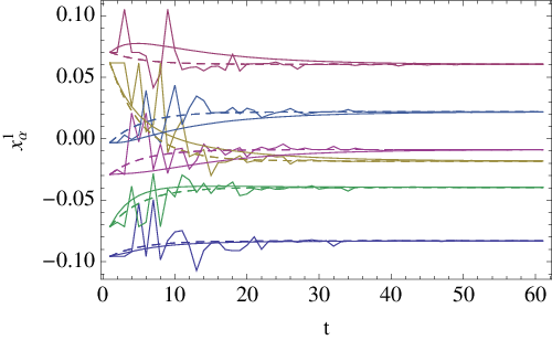
being the identity matrix, the all-one matrix, and . The eigenvalues of are , where and are the eigenvalues of and respectively. It follows that there are steady states associated with . These correspond to the conserved quantities . The remaining eigenvalues are . Because is doubly stochastic, and . So, and there is no instability. The rate of convergence is determined by the eigenvalue gap of the matrix . The network does not affect the wealth distribution but it gives the rate of convergence towards equilibrium. As expected, the larger the eigenvalue gap, the faster is the convergence. Graphs with good expansion properties are then associated with fast relaxation. Fig. 1 gives an example for the complete graph and the cycle graph on six vertices, using the same initial conditions. The numerical simulation is consistent with the mean field theory. The simulations are obtained taking Eq. (18) in discrete time. Moreover, we replace the matrix by a random matrix which chooses one pair of agents to interact in every time step. The pair is chosen from a uniform random distribution.
V.2 Heterogeneous dynamic preferences
It is worth considering an example with a slightly more complicated index of satisfaction,
| (19) |
where is a fixed but arbitary constant. The matrix represents a particular preference of the agent. It can be interpreted as an opinion about the exchange rates. Different agents might have different opinions. We assume that obeys the usual consistency conditions. Therefore, the choice of index in Eq. (19) is arbitrary. We will build a model where agents can learn the “market” exchange rates when they barter with other agents. This means, they will ultimately converge to some equilibrium prices . Therefore, for any of such equilibria, the preferences will be of the form:
One can easily show, from Eqs. (2), that thee space of equilibria of this model is the same as in the previous one: . Here we will expand, as in the previous case, around an homogeneous economy with . Note that even though in this model agents have time-dependent preferences out of equilibrium, they all converge to homogeneous preferences in equilibrium. This means that this model obeys the simplifying assumptions of Section II, and hence the final wealth distribution is independent of the non-equilibrium dynamics.
Now we need to provide a model of how the agents learn the new prices. We assume that, when two agents and find each other and make a trade, they update their respective matrices and as
| (20) |
for all . We have used Eqs. (8) and (9). This way of updating prices makes sure that the exchange rates always obey the consistency condition (see Eq.( 3)). Moreover, one could interpret such updating as an exchange of information between both agents: even though agents traded only two products, they “found out” about each other’s prices. The expectation of ’s internal matrix at the next time step is
| (21) | ||||
We have used the fact that the total probability per unit time of an encounter between agents and is given by . Taking expectations on both sides of Eq. (21) we get,
| (22) |
This can be seen as the evolution equation for the agent’s preferences.
We are now ready to work out the evolution equations for the scale invariant perturbations. Due to the consistency condition, we can always consider only the components of the prices. We can then define the following scale invariant variables for the price perturbations:
| (23) |
One finds that for the utility in Eq. (19), and for the homogeneous background, the amount of products traded is
| (24) | |||||
where it is understood that . By plugging Eq. (24) in Eq. (7), we get the equation for the perturbation in inventory:
| (25) | |||||
Next we derive the equation for the perturbations in the internal prices of the agents. In order to do this, we need the following result:
| (26) | |||||
where we have set without any loss of generality. We can now use Eq. (26) in Eq. (22) to get an expression for the price perturbations:
| (27) | ||||
where, again, . We can now analyze Eqs. (25) and (27) in order to prove the stability of the system. It is useful to diagonalize the matrix , as in the previous example. Recall that the price perturbation , since this is the perturbation of . However, we can just include as a spurious variable which will be conserved, i.e., . One can then show that Eqs. (25) and (27) can be written in matrix form as , where and
Here is the matrix with entries . Moreover,
When we take two products (), the two non-zero eigenvalues of are
| (28) | |||||
with and . It is straightforward to see that the real part of both eigenvalues is negative or zero. If we fix then the eigenvalue gap still determines the convergence rate as in the case of homogeneous preferences.
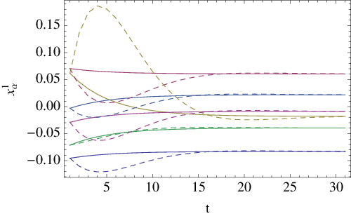
In Fig. 2, we compare the dynamics of this model with the simpler one of the previous section. We take the same initial conditions for the scale invariant perturbations, and fix the network to be the complete graph. We see that, as expected, the final state is the same for both models. However, for the changing preferences model, there are large oscillations due to the fact that the eigenvalues given in Eq. (28) are complex. Moreover, in the limit (wealth maximizers), these oscillations dominate and the system never equilibrates.
VI Conclusions
In this paper we have introduced a theory of linearized perturbations around a pure exchange economy. Our formalism is given in terms of a general index of satisfaction, and the probabilities of agents interacting on a network. We have shown that, if agents have static preferences, which are also homogeneous in any of the steady states, the final wealth distribution is independent of the dynamics of the non-equilibrium theory. In particular, it is completely determined in terms of the initial conditions, and it is independent of the probability and the network of interaction between agents. We have shown that the main effect of the network is to determine the relaxation time to equilibrium. We gave two examples where the relaxation times can be computed analytically. Moreover, we showed the agreement between the mean field theory technique and numerical simulations.
This work can be extended in a number of directions. First, it would be interesting to consider agents that have random changing preferences, or can speculate on exchange rates. Some simulations of this kind were conducted in [10] in the context of a centralized market. These speculations can lead to stochastic terms analog to the ones proposed in [7]. Finally, we have only considered agents making barter exchanges at a fixed time. An important component of the economy is that agents are able to make exchanges at different times. That is, we have contingency claims. It would be interesting to set up a similar perturbation theory involving such claims, and study the stability of the system.
Acknowledgments. The authors would like to thank Mike Brown, Jim Herriot, Stuart Kauffman, Zoe-Vonna Palmrose, and Lee Smolin, for helpful discussion. S. E. V. would like to thank Maes Bert for his kind hospitality at the Department of Chemistry of the University of Antwerp, where part of this work has been done. Research at Perimeter Institute for Theoretical Physics is supported in part by the Government of Canada through NSERC and by the Province of Ontario through MRI. Research at IQC is supported in part by DTOARO, ORDCF, CFI, CIFAR, and MITACS.
References
- [1] J. D. Farmer, J. Geanakoplos, The virtues and vices of equilibrium and the future of financial economics, Complexity 14 (2009): 11-38.
- [2] E. Smith and D. K. Foley, Journal of Economic Dynamics and Control, 2008, vol. 32, issue 1, pages 7-65.
- [3] J.-P. Bouchaud, J. D. Farmer, F. Lillo, How Markets Slowly Digest Changes in Supply and Demand. In Handbook of Financial Markets: Dynamics and Evolution, eds. Thorsten Hens and Klaus Schenk-Hoppe. Elsevier: Academic Press, 2008.
- [4] W. B. Arthur, Handbook of Computational Economics, Vol. 2: Agent-Based Computational Economics, K. Judd and L. Tesfatsion (Eds.), Elsevier/North-Holland, 2005.
- [5] L. Smolin, Time and symmetry in models of economic markets, February 2009. arXiv:0902.4274v1 [q-fin.GN]
- [6] A. Wilhite, Handbook of Computational Economics, Vol. 2: Agent-Based Computational Economics, K. Judd and L. Tesfatsion (Eds.), Elsevier/North-Holland, 2005.
- [7] J.-P. Bouchaud, M. Mézard, Physica A , 282, 2000, p.536-545.
- [8] D. Aldous, J. Fill, Reversible Markov Chains and Random Walks on Graphs, stat.berkeley.edu/˜aldous/RWG
- [9] A. Farkas, P. Rózsa, E. Stubnya, Linear Algebra Appl. 302–303 (1999) 423–433.
- [10] S. E. Vazquez, Scale Invariance, Bounded Rationality and Non-Equilibrium Economics, February 2009. arXiv:0902.3840v1 [q-fin.TR]