跳到论文正文
W Papers独立论文阅读器 arXiv:0904.1303 论文正文 计算阅读时间 · 0%
引用这篇论文根据当前论文元数据生成,正式投稿前建议核对。


License: arXiv.org perpetual non-exclusive license
arXiv:0904.1303v2 [gr-qc] 22 Apr 2009

Semiclassical analysis
of the
Loop Quantum Gravity volume operator:

Area Coherent States

C. Flori ††thanks: cecilia.flori@aei.mpg.de, ceciliaflori18@googlemail.com Affiliation:  MPI f. Gravitationsphysik, Albert-Einstein-Institut,Am Mühlenberg 1, 14476 Potsdam, Germany
Preprint AEI-2009-026
Abstract

We continue the semiclassical analysis of the Loop Quantum Gravity (LQG) volume operator that was started in the companion paper [24]. In the first paper we prepared the technical tools, in particular the use of complexifier coherent states that use squares of flux operators as the complexifier. In this paper, the complexifier is chosen for the first time to involve squares of area operators.

Both cases use coherent states that depend on a graph. However, the basic difference between the two choices of complexifier is that in the first case the set of surfaces involved is discrete, while, in the second it is continuous. This raises the important question of whether the second set of states has improved invariance properties with respect to relative orientation of the chosen graph in the set of surfaces on which the complexifier depends. In this paper, we examine this question in detail, including a semiclassical analysis.

The main result is that we obtain the correct semiclassical properties of the volume operator for i) artificial rescaling of the coherent state label; and ii) particular orientations of the 4- and 6-valent graphs that have measure zero in the group SO(3). Since such requirements are not present when analysing dual cell complex states, we conclude that coherent states whose complexifiers are squares of area operators are not an appropriate tool with which to analyse the semiclassical properties of the volume operator. Moreover, if one intends to go further and sample over graphs in order to obtain embedding independence, then the area complexifier coherent states should be ruled out altogether as semiclassical states.

I would like to dedicate this paper to my parents Elena Romani and Luciano Flori

1 Introduction

The volume operator in Loop Quantum Gravity11 1 See [2, 3] for recent books and [4] for recent reviews. (LQG) plays a central role in the quantum dynamics of the theory. Without it, it is not possible to define the Hamiltonian constraint operators [5], the Master constraint operators [6], or the physical Hamiltonian operators [7]. The same applies to truncated models of LQG such as Loop Quantum Cosmology (LQC) [8] which is believed to describe well the homogeneous sector of the theory. In LQC the quantum evolution of operators that correspond to classically-singular Dirac observables typically remains finite. This can be traced back to the techniques used to quantize inverse powers of the local volume that enter into the expression for the triad, co-triad and other types of coupling between geometry and geometry, or geometry and matter [5]. Specifically, such derived operators arise as commutators between holonomy operators and powers of the volume operator.

In view of its importance, it is of considerable interest to verify whether the classical limit of the LQG volume operator coincides with the classical volume. By this we mean that (i) the expectation value of the volume operator with respect to suitable semiclassical states which are peaked at a given point in phase space, coincides with the value of the classical volume at that phase space point, up to small corrections; and (ii) its fluctuations are small.

It should be remarked that there are actually two versions of the volume operator that have been discussed in the literature [9, 10]. These come from inequivalent regularisations of the products of operator-valued distributions that appear at intermediate stages. However, only the operator in [10] survives the consistency test of [11], namely, writing the volume in terms of triads which then are quantised using the commutator mentioned above, gives the same operator up to ℏ\hbar-corrections as that obtained from direct quantisation. This consistency check is important as otherwise we could not trust the triad and co-triad quantisations that enter the quantum dynamics.

A semiclassical analysis of the volume operator has not yet been carried out, although, in principle, suitable semiclassical (even coherent) states for LQG are available [12]. This is because the spectral decomposition (projection-valued measure) of the volume operator cannot be computed exactly in closed form. However, this is needed for exact, practical calculations. More precisely, the volume operator is the fourth root of a positive operator, QQ, whose matrix elements can be computed in closed form [13] but which cannot be diagonalised analytically.

In more detail, the volume operator has a discrete (that is, pure-point) spectrum and it attains a block-diagonal form where the blocks are labelled by the graphs and spin quantum numbers (labelling the edges of the graph) of spin-network functions (SNWF) [14]. SNWF form a convenient basis of the LQG Hilbert space [15] which carries a unitary representation of the spatial diffeomorphism group and the Poisson∗−{}^{\ast}-algebra of the elementary flux and holonomy variables [16]. The blocks turn out to be finite-dimensional matrices whose matrix elements can be expressed in terms of polynomials of 6j symbols. Fortunately, these complicated quantities can be avoided22 2 Notice that Racah’s formula provides a closed expression for the 6j symbol but it also involves implicit sums and factorials that involve large integers. These quickly becomes unmanageable, even numerically. by using a telescopic summation technique [17] related to the Elliot-Biedenharn identity [18], so that a manageable closed expression results. However, the size of these matrices grows exponentially with increasing spin quantum numbers and, since the expression for coherent states is a coherent superposition of SNWF’s with arbitrarily large spin quantum numbers, a numerical computation of the expectation value using the numerical diagonalisation techniques, that are currently being developed [19], is still a long way off.33 3 The coherent superposition contains a damping factor that suppresses large spins, and thereby large matrices, so that the complicated infinite series over spin quantum numbers can be truncated at finite values, making only negligible errors. However, the computational effort required is currently too high, even for supercomputers; for example, see the estimates of computation time reported in [19].

One way forward is to use the semiclassical perturbation theory developed in [20], and applied already in [21, 22]. The basic idea is quite simple. In practical calculations one needs the expectation value of QqQ^{q} where qq is a rational number in the range 0<q≤140<q\leq\frac{1}{4}. In order to attain that, one has to introduce the ‘perturbation operator’, X:=Q<Q>−1X:=\frac{Q}{<Q>}-1, where the expectation value <Q><Q> of the positive operator QQ is exactly computable. Notice that XX is bounded from below by −1-1. Then trivially <Qq>=<Q>q<[1+X]q><Q^{q}>=<Q>^{q}\;<[1+X]^{q}>. Now we exploit the existence of positive numbers pp such that the classical estimates 1+q​x−p​x2≤(1+x)q≤1+q​x1+qx-px^{2}\leq(1+x)^{q}\leq 1+qx are valid for all x≥−1x\geq-1. Finer estimates of this form involving arbitrary powers of xx are also available [21]. By virtue of the spectral theorem, this classical estimate survives at the quantum level and we have Y−≤Y≤Y+Y_{-}\leq Y\leq Y_{+} where Y+=1+q​X,Y−=Y+−p​X2,Y=(1+X)qY_{+}=1+qX,\;Y_{-}=Y_{+}-pX^{2},\;Y=(1+X)^{q}. It follows that <Y>∈[<Y+>−p<X2>,<Y+>]<Y>\in[<Y_{+}>-p<X^{2}>,<Y_{+}>]. However, <Y+>=1<Y_{+}>=1 and <X2>=[<Q2>−<Q>2]/<Q>2<X^{2}>=[<Q^{2}>-<Q>^{2}]/<Q>^{2} is proportional to the relative fluctuations of QQ, which are of order of ℏ\hbar [12]. It follows that to zeroth-order in ℏ\hbar we may replace <Qq><Q^{q}> by <Q>q<Q>^{q} which is computable, as are the error estimates in the way shown above.

The exact computation of <Q>,<Q2>,..<Q>,\;<Q^{2}>,\;.. is feasible, but it is still quite involved. At this point it is convenient to use the fact that (see [12]), to zeroth-order in ℏ\hbar, the computation of these expectation values (more generally, the expectation values of low-order polynomials in the flux operators) for S​U​(2)SU(2) spin-network states coincides with the corresponding calculations for U​(1)3U(1)^{3} spin networks. On the latter, the volume operator is even diagonal. Hence we conclude that, as long as we are only interested in the zeroth-order in ℏ\hbar contribution, we may evaluate the expectation value of the volume operator for a fictitious theory in which the non-Abelian group S​U​(2)SU(2) is replaced by the Abelian group U​(1)3U(1)^{3}. This dramatically simplifies all the calculations.

The coherent states developed so far for LQG have all been constructed using the complexifier method reviewed in [23]. This generalises the coherent-state construction for phase spaces that are cotangent bundles over a compact group; see [25]44 4 See also [26] for related ideas valid for Abelian gauge theories such as Maxwell theory or linearised gravity.. This construction involves computing the heat-kernel evolution of the delta distribution (which is the matrix element of the unit operator in the Schrödinger (position) representation) with respect to a generalized Laplace operator, called the ‘complexifier’, followed by a certain analytic continuation.

Now the unit operator in LQG can be written as a resolution of unity in terms of SNWF’s and, although the heat kernel is a damping operator, since the SNWF are not countable (the LQG Hilbert space is not separable), the resulting expression is not normalisable. However, it does give a well-defined distribution (in the algebraic dual of the finite linear span of SNWF’s) which can be conveniently written as a sum over cut–off states labelled by finite graphs. These states, called “shadows” in [25], are normalisable, and can be used to perform semiclassical calculations. Of course, one expects that the good semiclassical states will only be those cut–off states that are labelled by graphs which are sufficiently fine with respect to the classical three-metric to be approximated.

Thus the input in the semiclassical calculations consists in the choice of a complexifier and the choice of a graph. One may wonder why the complexifier has to be chosen a priori rather than being dictated by the dynamics of the theory: that is, why do the coherent states remain coherent under quantum time evolution? For example, for the harmonic oscillator, the complexifier is just the Laplacian on the real line.

The reason is two-fold. On the one hand, one could perform a constraint quantisation so that we are working at the level of the kinematical Hilbert space on which the quantum constraints have not yet been imposed. In this situation, all that is needed is to ensure that the volume operator, which is not gauge invariant (and thus does not preserve the physical Hilbert space), has a good classical limit on the kinematical Hilbert space. We would certainly not trust a constraint quantization for which even that was not true.

On the other hand, one could also work at the level of the physical Hilbert space, as outlined in [7]. Then, one would expect that the time evolution of any reasonable choice of complexifier coherent states with respect to the physical Hamiltonian should remain coherent (and peaked on the classical trajectory) for sufficiently short time intervals. Note that for interacting theories, even the simple example of the anharmonic oscillator, globally stable coherent states have yet to be found.

The choice of the complexifier will be guided by practical considerations: namely (i) it is diagonal on SNWF’s; and (ii) it is a damping operator that renders normalisable the heat-kernel evolution of the delta distribution restricted to a graph. Moreover, it should be gauge invariant under the S​U​(2)SU(2) gauge group. As for the choice of graph, for practical reasons one will use graphs that are topologically regular, that is, have a constant valence for each vertex. Indeed, the semiclassical calculations performed in [21, 22] were done using graphs of cubic topology, with good results.

The existing literature on such coherent states for LQG can be divided into two classes, depending on a certain structure that defines them. The first are gauge-covariant flux coherent states, which depend on collections of surfaces and path systems inside them [12]. The second are area coherent states, which also depend on collections of surfaces but involve area operators rather than flux operators [23]. In our companion paper [24] we have reviewed and generalised both constructions. In its most studied incarnations, the collection of surfaces involved in [12] is defined by a polyhedronal partition of the spatial manifold, while the collection used in [23] uses a plaquette of foliations of the spatial manifold.

The main objective of this series of two papers is to analyse the semiclassical properties of the volume operator with respect to both classes of coherent state. In [24] we employed the states of [12]. In this paper we employ the states of [23]. This exhausts all known coherent states for LQG. The result of our analysis is that, if we use the states [12], the correct semiclassical limit is attained with these states for n=6n=6 only. If instead we use the states [23], the correct semiclassical limit is attained only for: 1) artificial rescaling of the coherent state label; and 2) particular embeddings of the 4-valent and 6-valent graphs with respect to the set of surfaces on which the complexifier depends. However, the combinations of Euler angles for which such embeddings are attained have measure zero in SO(3), and are therefore negligible. Thus the area complexifier coherent states are not the correct tools with which to analyse the semiclassical properties of the volume operator.

If one wants to obtain embedding independence, a possible strategy is to sample over graphs (Dirichlet-Voronoi sampling [45]) as outlined in [12]. What this strategy amounts to is that, instead of singling out one particular coherent state ψγ,m\psi_{\gamma,m}—as defined in terms of a single graph γ\gamma—one considers an ensemble of coherent states constructed by averaging the one-dimensional projections P^γ,m\hat{P}_{\gamma,m} onto the states ψγ,m\psi_{\gamma,m} over a subset Γm\Gamma_{m} of the set of all allowed graphs. In other words, one considers a mixed state (with an associated density matrix) rather than a single coherent state. In such a way, if the subset Γm\Gamma_{m} is big enough, it can be shown ([12]) that it is possible to eliminate the embedding dependence (the ‘staircase problem’55 5 Roughly the staircase problem can be stated as follows. Consider an area operator A^S\hat{A}_{S} for a surface SS. If we compute the expectation value for A^S\hat{A}_{S} with respect to a coherent state ψγ,m\psi_{\gamma,m}, such that the surface SS intersects transversely one and only one edge ee of γ\gamma, then the expectation value of the area operator coincides with the classical value A⁡(m)A(m). However, if the surface SS lies transversally to the edges, then we do not obtain the correct classical limit.).

It is straightforward to deduce that the area complexifier coherent states cannot be used to construct embedding-independent, mixed coherent states because of condition 2) above. We thus claim that area complexifier coherent states should be ruled out as semiclassical states altogether if one wants to attain embedding independence. Instead one should use the flux coherent states, as was done in [12]. For such states we will show that the correct semiclassical limit is attained only for n=6n=6 . In other words, up to now, there are no semiclassical states known other than those with cubic-graph topology!

Thus the implication of our result for LQG is that the semiclassical sector of the theory is spanned by SNWF that are based on cubic graphs. This has some bearing for spin-foam models [28] which are supposed to be---but, so far, have not been proved to be---the path-integral formulation of LQG. Spin foams are certain state-sum models that are based on simplicial triangulations of four manifolds whose dual graphs are therefore 5-valent. The intersection of this graph with a boundary three-manifold is 4-valent, and therefore we see that spin-foam models, based on simplicial triangulations, correspond to boundary Hilbert spaces spanned by spin-network states based on 4-valent graphs only66 6 As an aside, whether this boundary Hilbert space of spin foams really can be interpreted as the 4-valent sector of LQG is a subject of current debate, even with the recent improvements [29] in the Barrett–Crane model [30]. There are two problems: first, the boundary connection predicted by spin foams does not coincide with the LQG connection [31]. Secondly, the 4-valent sector of the LQG Hilbert space is not a superselection sector for the holonomy flux algebra of LQG. In fact, the LQG representation is known not only to be cyclic but even irreducible [32]. Therefore the 4-valent sector is not invariant under the LQG algebra.. However, we have proved that the correct semiclassical states for analysing the semiclassical properties of the volume operator are the gauge covariant flux states. For such states, only those of cubic topology give the correct semiclassical value of the volume operator.

Even if the mismatches between the 4-valent sector of LQG and the boundary Hilbert space of spin foams could be surmounted, the result of our analysis seems to be that the boundary Hilbert space of current spin-foam models does not contain any semiclassical states! This apparently contradicts recent findings that the graviton propagator derived from spin-foam models is correct [33]. However, it is notable that these latter results only show that the propagator has the correct fall-off behaviour: the correct tensorial structure has not yet been verified.

One straightforward way of possibly repairing this situation is to generalise spin-foam models to allow for arbitrary—in particular, cubic—triangulations, as suggested in [34, 35].

In the present paper we will perform detailed calculations of the expectation value of the volume operator for the 4-, 6-, and 8-valent graphs using the area coherent states reviewed in [24]. The main difference between the flux coherent states and the area coherent states is that the former depend on a discrete set of flux operators while the latter depend on a continuous family of area operators. In particular, the surfaces on which the area operators depend fill all of space. Hence the question arises whether the area coherent states depend less severely on the relative orientation of the chosen cut-off graph with respect to the system of surfaces. Specifically, it would be interesting to know if the calculations of the expectation values are insensitive to Euclidean motions of the graph (translations and rotations) when the spatial metric to be approximated is the Euclidean one.

The structure of the paper is as follows. In Section 2 we calculate the expectation value for a general graph. The expectation value depends on the edge metric, already encountered in [24], which is close to diagonal when the edge lengths, δ\delta, are much larger than the lengths, ll, of the boundaries of the surfaces. In order to compute the off-diagonal metric entries we stick to the graphs defined in our companion paper as otherwise we encounter severe ‘bookkeeping’ problems. These graphs are dual to tetrahedronal, cubical and octahedronal triangulations, all of which derive from a cubulation of the spatial manifold, as discussed in [24]. One can expand the expectation value into a convergent power series in l/δl/\delta. We establish that, contrary to the results in [24], to zeroth-order in both ℏ\hbar and l/δl/\delta the correct expectation value is obtained for n=6n=6 and n=4n=4, but only for specific embeddings of the graph with respect to the surfaces on which the area operators depend. However, we show that such embeddings have measure zero in S​O​(3)SO(3). Moreover, by using the coherent states in [12] we also find that the graphs (4-, 6, and 8-valent) are all Euclidean invariant, up to sets of measure zero in S​O​(3)SO(3) and up to linear order in l/δl/\delta. Nonetheless, the embeddings with non-zero measure all fail to give the correct semiclassical value for the volume operator.

This shows that coherent states [12] are not the correct tools for analysing the semiclassical properties of the volume operators.

In Section 3 we perform an explicit calculation of the expectation value of the volume operator for 4-, 6-, and 8-valent graphs, including the higher-order effects in l/δl/\delta. This contribution is only Euclidean-invariant up to linear order. For each of these valences we first consider a graph constructed in terms of regular simplicial, cubical and octahedron cell complexes, as done in [24]. After that, we study the effects of rotations and translations.

In Section 4 we summarise our results and draw appropriate conclusions.

The more technical calculations have been transferred to an appendix in order not to distract from the line of argument in the main text.

2 Volume Operator Expectation Values for Area Coherent States

In this Section we compute the expectation value of the operator V^γ,v\hat{V}_{\gamma,v} for an arbitrary nn-valent vertex, vv, for the stack family coherent states using the replacement of S​U​(2)SU(2) by U​(1)3U(1)^{3}. This uses the calculational tools developed in [24], to which we refer for our notation. We may, therefore, replace the S​U​(2)SU(2) right-invariant vector fields by U​(1)3U(1)^{3} right-invariant vector fields XjeI​(v)=ihjI∂/∂hjIX^{j}_{e_{I}(v)}=ih^{j}_{I}\partial/\partial h^{j}_{I} acting on hIj:=Aj​(eI​(v))h^{j}_{I}:=A^{j}(e_{I}(v)). The crucial simplification is that these vector fields mutually commute. Their common eigenfunctions are the spin-network functions which, for U​(1)3U(1)^{3}, take the explicit form

Tγ,n​(A)=∏e∈E⁡(γ)∏j=13[Aj​(e)]njeT_{\gamma,n}(A)=\prod_{e\in E(\gamma)}\;\prod_{j=1}^{3}\;[A^{j}(e)]^{n_{j}^{e}} (2.1)

We will refer to them as ‘charge network states’ because the nje∈ℤn_{j}^{e}\in\mathbb{Z} are integer valued. Using the spectral theorem we may immediately write down the eigenvalues of V^γ,v\hat{V}_{\gamma,v} on Tγ,nT_{\gamma,n} as

λγ,n,v=ℓP3​|18​∑v∈eI∩eJ∩eK1≤I≤J≤K≤Nϵi​j​k​ϵ​(eI,eJ,eK)​[nieI​njeJ​nkeK]|\lambda_{\gamma,n,v}=\ell_{P}^{3}\sqrt{\Big|\frac{1}{8}\sum_{{v\in e_{I}\cap e_{J}\cap e_{K}}\atop{1\leq I\leq J\leq K\leq N}}\epsilon^{ijk}\epsilon(e_{I},e_{J},e_{K})\big[n^{e_{I}}_{i}\;n^{e_{J}}_{j}\;n^{e_{K}}_{k}\big]\Big|} (2.2)

What follows is subdivided into four parts. We begin by performing the calculation for a general graph. This leads to the inverse of the edge metric which, for large graphs, is beyond analytical control. In the second part we restrict the class of graphs, which lets us perform perturbative computations of the inverse of the edge metric. This gives a good approximation of the actual expectation value. In the third and fourth parts we consider the dependence of our results on the relative orientation of the graph with respect to the family of stacks.

2.1 General expectation value of the volume operator

In this Section we drop the graph label and set te​e′j​k:=δj​k​t​le​e′γ,t:=ℓP2/a2t^{jk}_{ee^{\prime}}:=\delta^{jk}\;tl^{\gamma}_{ee^{\prime}},\;t:=\ell_{P}^{2}/a^{2}. This gives a positive, symmetric bilinear form on vectors n:=(nje)e∈E⁡(γ),j=1,2,3n:=(n^{e}_{j})_{e\in E(\gamma),\;j=1,2,3} that is defined by t⁡(n,n′):=∑e,e′,j,knje​nk′e′​te​e′j​k=nT⋅t⋅n′t(n,n^{\prime}):=\sum_{e,e^{\prime},j,k}n^{e}_{j}n^{\prime e^{\prime}}_{k}t^{jk}_{ee^{\prime}}=n^{T}\cdot t\cdot n^{\prime}. We also set ZT⋅n:=∑e,jZj​(e)​njeZ^{T}\cdot n:=\sum_{e,j}Z^{j}(e)n^{e}_{j}.

The coherent state associated with an nn-valent graph in which more than one edge intersects a given plaquette SS, is as follows:

ψZ,γ=∑ne−12nT⋅t⋅neZT⋅nTγ,n\psi_{Z,\gamma}=\sum_{n}\;e^{-\frac{1}{2}n^{T}\cdot t\cdot n}\;\;e^{Z^{T}\cdot n}\;T_{\gamma,n} (2.3)

The norm of the coherent states is given by

||ψZ,γ||2=∑ne−nT⋅t⋅ne2​P⋅n||\psi_{Z,\gamma}||^{2}=\sum_{n}\;e^{-n^{T}\cdot t\cdot n}\;e^{2P\cdot n} (2.4)

where

Pj​(e)=i​∫e(Z−A)=:1b2​EjeP^{j}(e)=i\int_{e}(Z-A)=:\frac{1}{b^{2}}E^{e}_{j} (2.5)

The length parameter, bb, that appears here is generally different from the parameter, aa, that enters the classicality parameter t=ℓP2/a2t=\ell_{P}^{2}/a^{2}, as explained in [24].

The expectation value for the volume operator is

<Vv^>Z,γ=⟨ψZ,γ​Vγ,v^​ψZ,γ⟩‖ψZ,γ‖2=∑ne−nT⋅t⋅ne2​P⋅nλγ,v(n)‖ψZ,γ‖2<\hat{V_{v}}>_{Z,\gamma}=\frac{\langle\psi_{Z,\gamma}\hat{V_{\gamma,v}}\psi_{Z,\gamma}\rangle}{||\psi_{Z,\gamma}||^{2}}=\frac{\sum_{n}\;e^{-n^{T}\cdot t\cdot n}\;e^{2P\cdot n}\lambda_{\gamma,v}(n)}{||\psi_{Z,\gamma}||^{2}} (2.6)

where

λγ,v​(n)=ℓP3​|148​∑e∩e′∩e′′=vϵ⁡(e,e′,e′′)​dete​e′​e′′(n)|\lambda_{\gamma,v}(n)=\ell_{P}^{3}\sqrt{\Big|\frac{1}{48}\sum_{e\cap e^{\prime}\cap e^{\prime\prime}=v}\;\epsilon(e,e^{\prime},e^{\prime\prime})\;\det_{ee^{\prime}e^{\prime\prime}}(n)\Big|} (2.7)

are the eigenvalues of the volume operator V^γ,v\hat{V}_{\gamma,v}. We have introduced the notation

dete​e′​e′′(n):=ϵj​k​l​nje​nke′​nle′′\det_{ee^{\prime}e^{\prime\prime}}(n):=\epsilon^{jkl}\;n^{e}_{j}n^{e^{\prime}}_{k}n^{e^{\prime\prime}}_{l} (2.8)

The semiclassical limit of the volume operator is obtained from (2.6) in the limit of vanishing tt. That is, it is the zeroth-order in tt of the expansion of (2.6) in powers of tt. Since (2.6) converges slowly for small values of tt, we will perform a Poisson transform which replaces tt by 1t\frac{1}{t} which converges quickly. To this end, analogous to [21], we introduce the following variables

te:=te​e,Te:=te,xje:=Te​nje,yje​(x):=xje/Te,Cje:=Pje/Te,wje​(n):=nje/Te,Ae​e′j​k:=Ae​e′​δj​k:=te​e′te​te′t_{e}:=t_{ee},\;T_{e}:=\sqrt{t_{e}},\;x^{e}_{j}:=T_{e}n^{e}_{j},\;y^{e}_{j}(x):=x^{e}_{j}/T_{e},\;C^{e}_{j}:=P^{e}_{j}/T_{e},\;w^{e}_{j}(n):=n^{e}_{j}/T_{e},\;A_{ee^{\prime}}^{jk}:=A_{ee^{\prime}}\delta^{jk}:=\frac{t_{ee^{\prime}}}{\sqrt{t_{e}t_{e^{\prime}}}} (2.9)

Notice that the diagonal entries of AA equal unity. The off-diagonal ones, however, are bounded from above by unity by the Schwarz inequality applied to the scalar product defined by AA and are restricted to the six-dimensional subspace restricted to vectors with non-zero entries for the e,e′e,e^{\prime} components only.

Then (2.6) turns into

<Vv^>Z,γ=∑ne−xT⋅A⋅xe2​C⋅xλγ,v(y(x))∑ne−xT⋅A⋅xe2​C⋅x<\hat{V_{v}}>_{Z,\gamma}=\frac{\sum_{n}\;e^{-x^{T}\cdot A\cdot x}\;e^{2C\cdot x}\lambda_{\gamma,v}(y(x))}{\sum_{n}\;e^{-x^{T}\cdot A\cdot x}\;e^{2C\cdot x}} (2.10)

Applying the Poisson transform to (2.10) we obtain (recall N:=|E⁡(γ)|N:=|E(\gamma)|)

<Vv^>Z,γ=∑n∫ℝ3​Nd3​Nxe−2πiw(n)T⋅xe−xT⋅A⋅xe2​C⋅xλγ,v(y(x))∑n∫ℝ3​Nd3​Nxe−2πiw(n)T⋅xe−xT⋅A⋅xe2​C⋅x<\hat{V_{v}}>_{Z,\gamma}=\frac{\sum_{n}\;\int_{\mathbb{R}^{3N}}\;d^{3N}x\;e^{-2\pi iw(n)^{T}\cdot x}e^{-x^{T}\cdot A\cdot x}\;e^{2C\cdot x}\lambda_{\gamma,v}(y(x))}{\sum_{n}\;\int_{\mathbb{R}^{3N}}\;d^{3N}x\;e^{-2\pi iw(n)^{T}\cdot x}e^{-x^{T}\cdot A\cdot x}\;e^{2C\cdot x}} (2.11)

In order to perform the Gaussian integrals in (2.11) we notice that, by construction, AA is a positive-definite, finite-dimensional matrix, so that its square root, A\sqrt{A}, and its inverse are well defined via the spectral theorem. Hence we introduce as new integration variables

zje:=∑e′,k(A)j​ke​e′xke′,yje(z)=1Texje=1Te∑e′​k([A]−1])j​ke​e′zke′z^{e}_{j}:=\sum_{e^{\prime},k}(\sqrt{A})^{ee^{\prime}}_{jk}x^{e^{\prime}}_{k},\;y^{e}_{j}(z)=\frac{1}{T_{e}}x^{e}_{j}=\frac{1}{T_{e}}\sum_{e^{\prime}k}\big([\sqrt{A}]^{-1}]\big)^{ee^{\prime}}_{jk}z^{e^{\prime}}_{k} (2.12)

The Jacobian from the change of variables drops out in the fraction, and (2.11) becomes

<Vv^>Z,γ=∑n∫ℝ3​Nd3​Nze2​(C−2​π​i​w​(n))T⋅A−1⋅ze−zT⋅zλγ,v(y(z))∑n∫ℝ3​Nd3​Nze2​(C−2​π​i​w​(n))T⋅A−1⋅ze−zT⋅z<\hat{V_{v}}>_{Z,\gamma}=\frac{\sum_{n}\;\int_{\mathbb{R}^{3N}}\;d^{3N}z\;e^{2(C-2\pi iw(n))^{T}\cdot\sqrt{A}^{-1}\cdot z}e^{-z^{T}\cdot z}\;\lambda_{\gamma,v}(y(z))}{\sum_{n}\;\int_{\mathbb{R}^{3N}}\;d^{3N}z\;e^{2(C-2\pi iw(n))^{T}\cdot\sqrt{A}^{-1}\cdot z}e^{-z^{T}\cdot z}} (2.13)

Now one would like to shift zz into the complex domain by A−1​(C−i​π​w)\sqrt{A}^{-1}(C-i\pi w) and then perform the ensuing Gaussian integral. This is unproblematic for the denominator of (2.11) which is analytic in zz; however, the numerator is not. The careful analysis in [21] shows the existence of branch cuts in ℂ3​N\mathbb{C}^{3N} of the fourth-root function involved. In turn, this shows that, in the semiclassical limit, both numerator and denominator are dominated by the n=0n=0 term while the remaining terms in the series are of order ℏ∞\hbar^{\infty} (i.e they decay as exp(−kn/t),t=ℓP2/a2\exp(-k_{n}/t),\;t=\ell_{P}^{2}/a^{2} for some kn>0,limn→∞kn=∞k_{n}>0,\;\lim_{n\to\infty}k_{n}=\infty). See [21] for the details.

The upshot is that to any polynomial order in ℏ\hbar we may replace (2.13) by

<Vv^>Z,γ=∫ℝ3​Nd3​Nze−zT⋅zλγ,v(y(z+A−1C))∫ℝ3​Nd3​Nze−zT⋅z<\hat{V_{v}}>_{Z,\gamma}=\frac{\int_{\mathbb{R}^{3N}}\;d^{3N}z\;e^{-z^{T}\cdot z}\;\lambda_{\gamma,v}(y(z+\sqrt{A}^{-1}C))}{\int_{\mathbb{R}^{3N}}\;d^{3N}z\;e^{-z^{T}\cdot z}} (2.14)

which is now defined unambiguously because the argument of the fourth root is the square of a real number.

The denominator of (2.14) simply equals π3​N\sqrt{\pi}^{3N}. Therefore, the only ℏ\hbar-dependence of (2.14) lies in the numerator in the function λγ,v\lambda_{\gamma,v}. We now note that the eigenvalues of the volume operator come with a factor of ℓP3\ell_{P}^{3}, as displayed in (2.7). Pulling it under the square root into the modulus, and noticing that the modulus is a third-order polynomial in yy, we see that

λγ,v​(y⁡(z+A−1​C))=|148​∑e∩e′∩e′′=vϵ⁡(e,e′,e′′)​dete,e′,e′′(ℓP2​y​(z+A−1​C))|\lambda_{\gamma,v}\big(y(z+\sqrt{A}^{-1}C)\big)=\sqrt{\Big|\frac{1}{48}\sum_{e\cap e^{\prime}\cap e^{\prime\prime}=v}\epsilon(e,e^{\prime},e^{\prime\prime})\det_{e,e^{\prime},e^{\prime\prime}}\big(\ell_{P}^{2}y(z+\sqrt{A}^{-1}C)\big)\Big|} (2.15)

where we have

[ℓP2​y​(z+A−1)​C]je\displaystyle\big[\ell_{P}^{2}y(z+\sqrt{A}^{-1})C\big]^{e}_{j} =\displaystyle= ℓP2Te​∑e′,k[A−1]j​ke​e′​[z+A−1​C]ke′\displaystyle\frac{\ell_{P}^{2}}{T_{e}}\sum_{e^{\prime},k}\big[\sqrt{A}^{-1}\big]^{ee^{\prime}}_{jk}\big[z+\sqrt{A}^{-1}C\big]^{e^{\prime}}_{k} (2.16)
=\displaystyle= tTe​∑e′,k(a2​t​[A−1]j​ke​e′​zke′+tTe′​[A−1]j​ke​e′​(ab)2​Eke′)\displaystyle\frac{\sqrt{t}}{T_{e}}\sum_{e^{\prime},k}\;\Big(a^{2}\sqrt{t}\big[\sqrt{A}^{-1}\big]^{ee^{\prime}}_{jk}z^{e^{\prime}}_{k}+\frac{\sqrt{t}}{T_{e^{\prime}}}\big[A^{-1}\big]^{ee^{\prime}}_{jk}\Big(\frac{a}{b}\Big)^{2}E^{e^{\prime}}_{k}\Big)

where (2.5) has been used in the last line.

To extract the leading order in tt of (2.14) is now easy. First note that the matrix elements of both AA and Te/tT_{e}/\sqrt{t} are of order unity. Since aa is some macroscopic length scale, the first term that is proportional to zz in (2.16) is therefore of order t\sqrt{t}, while the second is of zeroth-order in tt. Therefore F:=λγ,v​(y⁡(z+A−1​C))F:=\lambda_{\gamma,v}\big(y(z+\sqrt{A}^{-1}C)\big) is of the form

F⁡(z​t)=Q+P⁡(z​t)4F(z\sqrt{t})=\root 4 \of{Q+P(z\sqrt{t})} (2.17)

where PP is a certain sixth-order polynomial in z​tz\sqrt{t} with no zeroth-order term, while QQ is independent of zz. Moreover, Q+P⁡(z​t)Q+P(z\sqrt{t}) is non-negative for all zz because it is the square of a third-order polynomial in zz. In particular, this holds at z=0z=0, and therefore QQ is also a non-negative number. Then, provided Q>0Q>0, we can define

f⁡(z​t):=F⁡(z​t)Q4=:1+R⁡(z​t)4f(z\sqrt{t}):=\frac{F(z\sqrt{t})}{\root 4 \of{Q}}=:\root 4 \of{1+R(z\sqrt{t})} (2.18)

where RR is a sixth-order polynomial with no zeroth-order term which is bounded from below by −1-1. Now, as in [20], we exploit the existence of r>0r>0 such that

1+14​R−r​R2≤f≤1+14​R1+\frac{1}{4}R-rR^{2}\leq f\leq 1+\frac{1}{4}R (2.19)

for all R≥−1R\geq-1. Inserting this estimate into (2.14) we can bound the integral from above and below because the Gaussian is positive. The integrals over RR and R2R^{2} are finite and are at least of order tt because odd powers of zz do not contribute to the Gaussian integral.

It follows that to zeroth-order in tt we have

<Vv^>Z,γ=|148​∑e∩e′∩e′′=vϵ⁡(e,e′,e′′)​dete,e′,e′′(Y)|<\hat{V_{v}}>_{Z,\gamma}=\sqrt{\Big|\frac{1}{48}\sum_{e\cap e^{\prime}\cap e^{\prime\prime}=v}\;\epsilon(e,e^{\prime},e^{\prime\prime})\;\det_{e,e^{\prime},e^{\prime\prime}}(Y)\Big|} (2.20)

where

Yje:=(ab)2​∑e′,ktTe​Te′​[A−1]j​ke​e′​Eke′Y^{e}_{j}:=\Big(\frac{a}{b}\Big)^{2}\sum_{e^{\prime},k}\;\frac{t}{T_{e}T_{e^{\prime}}}\;[A^{-1}]^{ee^{\prime}}_{jk}E^{e^{\prime}}_{k} (2.21)

This is as far as we can go with the calculation for a general graph. Notice that the inverse of the edge metric appears in this expression and, for a general graph, this is beyond analytical control. Therefore we will now make restrictions on the graph so as to analyse (2.21) further.

2.2 Simplifying assumptions

The assumptions about the class of graphs to be considered are as follows:

  • 1.

    Coordinate Chart
    The graph, the region RR and the families of stacks lie in a common coordinate chart X:ℝ3→σX:\;\mathbb{R}^{3}\to\sigma. This is not a serious restriction because the general situation may be reduced to this one by appropriately restricting attention to the various charts of an atlas that covers σ\sigma.

  • 2.

    Tame Graphs
    We assume that the graph is tame with respect to the stacks. By this we mean that for each direction II, and each stack α\alpha, a given edge, ee, of the graph enters and leaves that stack at most once. This means that the graph does not ‘wiggle’ too much on the scale of the plaquettes. Analytically, it means that lNI​α​γl^{I\alpha\gamma}_{N} vanishes whenever |Ne|≥2|N_{e}|\geq 2 for any ee, and that, for given ee, the number lNI​α​γl^{I\alpha\gamma}_{N} is non-vanishing at most for either Ne=+1N_{e}=+1 or Ne=−1N_{e}=-1 but, not both, and independently of α\alpha. Finally, it means that the sets SNI​α​γS^{I\alpha\gamma}_{N} are connected.

  • 3.

    Coarse Graphs
    We assume that the graph is much coarser than the plaquettation in the sense that any edge intersects many different stacks in at least one direction II.

  • 4.

    Non-Aligned Graphs
    We exclude the possibility that distinct edges are ‘too aligned’ with each other in the sense that the number of stacks that they commonly traverse is much smaller than the number of stacks that they individually traverse .

Pictorially, the situation therefore typically looks as in figure 1.

Refer to caption
Figure 1: Example of a tame, course and non-aligned graph

A consequence of the tameness, coarseness and ‘alignedness’ assumption is that |te,e′γ|≪teγ=te​eγ,te′γ=te′​e′γ|t^{\gamma}_{e,e^{\prime}}|\ll t^{\gamma}_{e}=t^{\gamma}_{ee},\;t^{\gamma}_{e^{\prime}}=t^{\gamma}_{e^{\prime}e^{\prime}} for all e,e′e,e^{\prime}, as is immediately obvious from the formulae displayed in our companion paper because the number of stacks with |Ne|=|Ne′|=1|N_{e}|=|N_{e^{\prime}}|=1 will be very much smaller than the number of stacks with |Ne|=1,Ne′=0|N_{e}|=1,N_{e^{\prime}}=0 or |Ne′|=1,Ne=0|N_{e^{\prime}}|=1,N_{e}=0. Hence the edge metric will be almost diagonal. This is important because we need its inverse, which can only be calculated with good approximation (that is, for large, semiclassically relevant graphs) if it is almost diagonal. The graphs that we will eventually consider are embeddings of subgraphs dual to tetrahedronal, cubical or octahedronal triangulations of ℝ3\mathbb{R}^{3}. These correspond to embeddings of regular 44-,66-,88-valent lattices, which ensures the non-alignedness property.

Thus, without loss of generality, we may choose the stacks and plaquettes as follows. Using the availability of the chart X:ℝ3→σ;s→X⁡(s)X:\;\mathbb{R}^{3}\to\sigma;\;s\to X(s) we consider the foliations FIF^{I} defined by the leaves LI​t:=XtI​(ℝ2)L_{It}:=X^{I}_{t}(\mathbb{R}^{2}) where for ϵI​J​K=1\epsilon_{IJK}=1 we set XtI​(u1,u2):=X⁡(sI:=t,sJ:=u1,sK:=u2)X^{I}_{t}(u^{1},u^{2}):=X(s^{I}:=t,\;s^{J}:=u^{1},s^{K}:=u^{2}). The stacks are labelled by α=(α1,α2)∈ℤ2\alpha=(\alpha^{1},\alpha^{2})\in\mathbb{Z}^{2}. The corresponding plaquettes are given by pα​tI={XtI([α+u]l);u∈[0,1)2}p^{I}_{\alpha t}=\{X^{I}_{t}([\alpha+u]l);\;u\in[0,1)^{2}\} where l>0l>0 is a positive number.

Likewise, using the availability of the chart, we take the edges of the graph to be embeddings of straight lines in ℝ3\mathbb{R}^{3} (with respect to the Euclidean background metric available there), that is, e⁡(t)=X⁡(se+ve​δ​t)e(t)=X(s_{e}+v_{e}\delta t) where vev_{e} is a vector in ℝ3\mathbb{R}^{3} and e⁡(0)=X⁡(se)e(0)=X(s_{e}) defines the beginning point of the edge.

After these preparations, we can now analyse (2.20) and (2.21) further. Recall that

Eje=∑α,I∫d​t​Ej​(ptα​I)​σ​(ptα​I,e)E^{e}_{j}=\sum_{\alpha,I}\;\int\;dt\;E_{j}(p^{\alpha I}_{t})\sigma(p^{\alpha I}_{t},e) (2.22)

and

te​e′γ=∑α​I∫d​t​σ​(ptα​I,e)​σ​(ptα​I,e′)t^{\gamma}_{ee^{\prime}}=\sum_{\alpha I}\int\;dt\;\sigma(p^{\alpha I}_{t},e)\;\sigma(p^{\alpha I}_{t},e^{\prime}) (2.23)

By the assumption about the graphs made above, the signed intersection number takes at most the numbers ±1\pm 1 and independently of α\alpha, so that σ​(ptα​I,e)2=σeI​σ​(ptα​I,e)\sigma(p^{\alpha I}_{t},e)^{2}=\sigma^{I}_{e}\sigma(p^{\alpha I}_{t},e) for certain σeI=±1\sigma^{I}_{e}=\pm 1 which takes the value +1+1 if the orientation of ee agrees with that of the leaves of the foliation, −1-1 if it disagrees, and 00 if it lies inside a leaf. If we assume that the electric field EjaE^{a}_{j} is slowly varying at the scale of the graph (and hence at the scale of the plaquettes as well) then we may write

Eje≈∑Ite​eγ​σeI​Ej​(pvI)E^{e}_{j}\approx\sum_{I}t^{\gamma}_{ee}\sigma^{I}_{e}E_{j}(p^{I}_{v}) (2.24)

where pvI=ptI​(v)αI​(v)​Ip^{I}_{v}=p^{\alpha_{I}(v)I}_{t_{I}(v)} and vv is the vertex at which ee is adjacent and which is under consideration in Vγ,vV_{\gamma,v}. It follows that (2.21) can be written as

Yje=(ab)2​∑e′,ktTe​Te′​[A−1]j​ke​e′​∑Ite′​e′γ​σeI​Ek​(pvI)=(ab)2​∑e′te′​e′γte​eγ​[A−1]e​e′​∑IσeI​Ej​(pvI)Y^{e}_{j}=\Big(\frac{a}{b}\Big)^{2}\sum_{e^{\prime},k}\;\frac{t}{T_{e}T_{e^{\prime}}}\;\big[A^{-1}\big]^{ee^{\prime}}_{jk}\sum_{I}t^{\gamma}_{e^{\prime}e^{\prime}}\sigma^{I}_{e}E_{k}(p^{I}_{v})=\Big(\frac{a}{b}\Big)^{2}\sum_{e^{\prime}}\;\sqrt{\frac{t^{\gamma}_{e^{\prime}e^{\prime}}}{t^{\gamma}_{ee}}}\;\big[A^{-1}\big]^{ee^{\prime}}\sum_{I}\sigma^{I}_{e}E_{j}(p^{I}_{v}) (2.25)

where we have used Te2=t​te​eγT_{e}^{2}=tt^{\gamma}_{ee}.

Now, by construction, A=1+BA=1+B with BB off-diagonal and with small entries

Be​e′=te​e′γte​eγ​te′​e′γB_{ee^{\prime}}=\frac{t^{\gamma}_{ee^{\prime}}}{\sqrt{t^{\gamma}_{ee}t^{\gamma}_{e^{\prime}e^{\prime}}}} (2.26)

which are of the order of l/δl/\delta since two distinct edges will typically only remain in the same stack for a parameter length ll, while the parameter length of an edge is δ\delta. Now notice that under the assumptions we have made, we have le​e′γ=0l^{\gamma}_{ee^{\prime}}=0 if e,e′e,e^{\prime} are not adjacent. Define SeS_{e} to be the subset of edges which are adjacent to ee. Then

‖B​x‖2\displaystyle||Bx||^{2} =\displaystyle= ∑e∑e′,e′′∈Sexe′​Be′​e​Be​e′′​xe′′\displaystyle\sum_{e}\sum_{e^{\prime},e^{\prime\prime}\in S_{e}}x_{e^{\prime}}B_{e^{\prime}e}B_{ee^{\prime\prime}}x_{e^{\prime\prime}} (2.27)
≤\displaystyle\leq [supe,e′Be​e′2]​∑e[∑e′∈Sexe′]2\displaystyle[\sup_{e,e^{\prime}}B_{ee^{\prime}}^{2}]\;\sum_{e}\;\big[\sum_{e^{\prime}\in S_{e}}\;x_{e^{\prime}}\big]^{2}
≤\displaystyle\leq (lδ)2​∑e[(∑e′∈Se12)1/2​(∑e′∈Sexe′2)1/2]2\displaystyle\Big(\frac{l}{\delta}\Big)^{2}\sum_{e}\;\Big[\big(\sum_{e^{\prime}\in S_{e}}1^{2}\big)^{1/2}\;\big(\sum_{e^{\prime}\in S_{e}}x_{e^{\prime}}^{2}\big)^{1/2}\Big]^{2}
≤\displaystyle\leq (lδ)2​M​∑e∑e′∈Sexe′2\displaystyle\Big(\frac{l}{\delta}\Big)^{2}\;M\;\sum_{e}\;\sum_{e^{\prime}\in S_{e}}x_{e^{\prime}}^{2}
=\displaystyle= (lδ)2​M​∑e′xe′2​∑eχSe​(e′)\displaystyle\Big(\frac{l}{\delta}\Big)^{2}\;M\;\sum_{e^{\prime}}x_{e^{\prime}}^{2}\;\sum_{e}\chi_{S_{e}}(e^{\prime})
≤\displaystyle\leq (lδ)2​M2​‖x‖2\displaystyle\Big(\frac{l}{\delta}\Big)^{2}\;M^{2}\;||x||^{2}

Here, in the second step we estimated the matrix elements of BB from above; in the third step we applied the Schwarz inequality; in the fourth step we estimated |Se|≤M|S_{e}|\leq M, where MM is the maximal valence of a vertex in γ\gamma; and in the sixth step we exploited the symmetry

χSe(e′)={1:e′∩e≠∅0:e′∩e=∅=χSe′(e)\chi_{S_{e}}(e^{\prime})=\left\{\begin{array}[]{cc}1&:\;\;e^{\prime}\cap e\not=\emptyset\\ 0&:\;\;e^{\prime}\cap e=\emptyset\end{array}\right.=\chi_{S_{e}^{\prime}}(e) (2.28)

as well as the definition of the norm of xx.

It follows that for l/δ<Ml/\delta<M, BB is bounded from above by unity. Therefore, the geometric series A−1=1+∑n=1∞(−B)nA^{-1}=1+\sum_{n=1}^{\infty}(-B)^{n} converges in norm. Hence we are able to consider the effects of a non-diagonal edge metric up to arbitrary order, nn, in l/δl/\delta. Here we will consider n=1n=1 only and write A−1=1−(A−1)=2⋅1−AA^{-1}=1-(A-1)=2\cdot 1-A. But before considering corrections from the off-diagonal nature of AA notice that, to zeroth-order in l/δl/\delta, equation (2.25) becomes simply

Yje=(ab)2​∑IσeI​Ej​(pvI)Y^{e}_{j}=\Big(\frac{a}{b}\Big)^{2}\sum_{I}\sigma^{I}_{e}E_{j}(p^{I}_{v}) (2.29)

Inserting (2.29) into (2.20) we find

<Vv^>Z,γ≈(ab)3|det(E)​(v)||148​∑e∩e′∩e′′=vϵ⁡(e,e′,e′′)​dete,e′,e′′(σ)​det(pv)|<\hat{V_{v}}>_{Z,\gamma}\,\approx\,\Big(\frac{a}{b}\Big)^{3}\sqrt{\big|\det(E)(v)\big|}\;\sqrt{\Big|\frac{1}{48}\sum_{e\cap e^{\prime}\cap e^{\prime\prime}=v}\;\epsilon(e,e^{\prime},e^{\prime\prime})\;\det_{e,e^{\prime},e^{\prime\prime}}(\sigma)\;\det(p_{v})\Big|} (2.30)

where

det(pv)=13!ϵI​J​Kϵa​b​c∫[0,1)2d2una​tI​(v)αI​(v)​I(u)∫[0,1)2d2unb​tJ​(v)αJ​(v)​I(u)∫[0,1)2d2unc​tK​(v)αK​(v)​I(u)\det(p_{v})=\frac{1}{3!}\epsilon_{IJK}\epsilon^{abc}\;\int_{[0,1)^{2}}\;d^{2}u\;n_{at_{I}(v)}^{\alpha_{I}(v)I}(u)\;\int_{[0,1)^{2}}\;d^{2}u\;n_{bt_{J}(v)}^{\alpha_{J}(v)I}(u)\;\int_{[0,1)^{2}}\;d^{2}u\;n_{ct_{K}(v)}^{\alpha_{K}(v)I}(u) (2.31)

On recalling that na​tα​I=ϵa​b​c​Xα​t,u1I​b​Xα​t,u2I​cn^{\alpha I}_{at}=\epsilon_{abc}X^{Ib}_{\alpha t,u^{1}}X^{Ic}_{\alpha t,u^{2}} with Xα​tI​a​(u)=Xa​(sI=t,sJ=α1+l​u1,sK=α2+l​u2)X^{Ia}_{\alpha t}(u)=X^{a}(s^{I}=t,s^{J}=\alpha^{1}+lu^{1},s^{K}=\alpha^{2}+lu^{2}) for ϵI​J​K=1\epsilon_{IJK}=1, we find

det(pv)≈l6​[det(∂X⁡(s)/∂s)]X⁡(s)=v\det(p_{v})\approx l^{6}\big[\det(\partial X(s)/\partial s)\big]_{X(s)=v} (2.32)

Hence (2.30) becomes

<Vv^>Z,γ≈(a​lb)3|det(E)​(v)||[det(∂X(s)/∂s)]X⁡(s)=v||148​∑e∩e′∩e′′=vϵ⁡(e,e′,e′′)​dete,e′,e′′(s)|<\hat{V_{v}}>_{Z,\gamma}\approx\Big(\frac{al}{b}\Big)^{3}\sqrt{\big|\det(E)(v)\big|}\;\Big|\big[\det(\partial X(s)/\partial s)\big]_{X(s)=v}\Big|\;\sqrt{\Big|\frac{1}{48}\sum_{e\cap e^{\prime}\cap e^{\prime\prime}=v}\;\epsilon(e,e^{\prime},e^{\prime\prime})\;\det_{e,e^{\prime},e^{\prime\prime}}(s)\Big|} (2.33)

We can draw an important conclusion from expression (2.33). Namely, the first three factors approximate the classical volume Vv​(E)V_{v}(E) as determined by EE of an embedded cube with parameter volume (a​l/b)3(al/b)^{3}. When we sum (2.33) over the vertices of γ\gamma, which have a parameter distance, δ\delta, from each other where l≪δl\ll\delta by assumption, then the volume expectation value only has a chance to approximate the classical volume when the graph is such that δ=a​l/b\delta=al/b, or δ/l=a/b\delta/l=a/b. This could never have been achieved for b=ab=a and explains why we had to rescale the labels of the coherent states by (a/b)2(a/b)^{2} while keeping the classicality parameter at t=ℓP2/a2t=\ell_{P}^{2}/a^{2}. See our companion paper for a detailed discussion. There we also explained why one must have δ/l\delta/l actually equal to a/ba/b and not just of the same order: While one could use this in order to favour other valences of the volume operator, the expectation value of other geometrical operators such as area and flux would be incorrect.

Assuming δ/l=a/b\delta/l=a/b we write (2.33) as

<Vv^>Z,γ=:Vv(E)Gγ,v<\hat{V_{v}}>_{Z,\gamma}=:V_{v}(E)\;G_{\gamma,v} (2.34)

thereby introducing the graph geometry factor Gγ,vG_{\gamma,v}. It does not carry any information about the phase space, only about the embedding of the graph relative to the leaves of the three-foliations. From the fact that (2.34) reproduces the volume of a cube up to a factor, we may already anticipate that the geometry factor will be close to unity for, at most, a cubic graph. Whether this holds for an arbitrary orientation of the graph with respect to the stack family will occupy a large part of the analysis which follows.

2.3 Preliminary analysis of the graph geometry factor

We start by investigating the behaviour of the graph geometry factor Gγ,vG_{\gamma,v} under diffeomorphisms, φ\varphi, of σ\sigma, that is, under Gγ,v↦Gφ⁡(γ),φ⁡(v)G_{\gamma,v}\mapsto G_{\varphi(\gamma),\varphi(v)} while the linearly-independent families of stacks are left untouched. This will answer the question of how much the geometry factor depends on the relative orientation of the graph with respect to the stacks.

In fact, the orientation factor ϵ⁡(e,e′,e′′)\epsilon(e,e^{\prime},e^{\prime\prime}) is invariant under diffeomorphisms of the spatial manifold σ\sigma. The signature factor

dete,e′​e′′(σ)=ϵI​J​K​σeI​σe′J​σe′′K\det_{e,e^{\prime}e^{\prime\prime}}(\sigma)=\epsilon_{IJK}\sigma^{I}_{e}\sigma^{J}_{e^{\prime}}\sigma^{K}_{e^{\prime\prime}} (2.35)

is obviously invariant under any diffeomorphism that preserves the foliations FIF^{I}, i.e. which map leaves onto leaves, because

σeI=12​∫ed​xa​ϵa​b​c​∫LI​td​yb∧d​yc​δ​(x,y)\sigma^{I}_{e}=\frac{1}{2}\int_{e}dx^{a}\,\epsilon_{abc}\int_{L_{It}}dy^{b}\wedge dy^{c}\delta(x,y) (2.36)

where LI​tL_{It} is any leaf in tt which intersects ee transversely. Since we consider graphs whose edges are embedded lines in ℝ3\mathbb{R}^{3} with the same embedding that defines the stacks, it follows that the geometry factor is invariant under any embedded global translations in ℝ3\mathbb{R}^{3}.

Next, since global rescaling in ℝ3\mathbb{R}^{3} preserves the foliations and the topological invariant (2.36), the geometry factor is also invariant under embedded global rescalings of ℝ3\mathbb{R}^{3}. Finally, any embedded global rotations of ℝ3\mathbb{R}^{3} that preserves all the orientation factors σeI\sigma^{I}_{e} will leave the geometry factors invariant. Since the orientation factors only take the values +1,−1,0+1,-1,0 (depending on whether an edge agrees, disagrees with the orientation of the leaves, or lies within a leaf), there will be a vast range of Euler angles for which this condition is satisfied, if the graph is an embedded, regular lattice of constant valence77 7 In fact, for a random graph we may also have rotational invariance on large scales.. Hence, in order to check whether the geometry factor is rotationally invariant under any rotation we need only worry about those rotations which lead to changes in the σeI\sigma^{I}_{e}. Likewise, if we rotate a graph which is dual to a polyhedronal complex, we expect that the expectation value remains invariant as long as the graph remains dual to the complex.

Fortunately, using the explicit formulae derived for the edges and vertices for n=4n=4-, 66-, 88-valent graphs displayed in [24] we can calculate the σeI\sigma^{I}_{e} for each edge ee. Intuitively, it is clear, that whenever many of the σeI\sigma^{I}_{e} change from +1+1 to −1-1, we can expect a drastic change of the expectation value. However, one has to take into account the combined effect of these changes, and this is what makes rotational invariance possible. As a first step we determine the action of a rotation on the sign factors.

2.4 Explicit calculation of the σeI\sigma^{I}_{e} terms

In what follows we discuss the cases that show a drastic change in the value of dete,e′,e′′(σ)=ϵI​J​KσeIσe′Jσe′′k\det_{e,e^{{}^{\prime}},e^{{}^{\prime\prime}}}(\sigma)=\epsilon_{IJK}\sigma_{e}^{I}\sigma_{e^{{}^{\prime}}}^{J}\sigma_{e^{{}^{\prime\prime}}}^{k} caused by a change in the values of σeI\sigma^{I}_{e}. To carry out this calculation we will perform a rotation of each of the three different types of lattice analysed so far: namely, the 44-, 66- and 88-valent lattices. These rotations will be parameterised by Euler angles and will be centred at a particular vertex of the lattice, for example V0V_{0}. The effects of a rotation will depend on the distance of the vertices from the centre of the rotation. In fact, the position of each vertex in the lattice after rotation will depend on both the distance from the centre of the rotation and the Euler angles used in the rotation. Fortunately, the values of the terms σeI\sigma^{I}_{e} will not depend on the former but only on the latter.

This is easy to see since the value of σeI\sigma^{I}_{e} can be either 1, -1 or 0 depending on whether the edge is outgoing, ingoing, or lies on the plaquette in the direction II. Thus it will only depend on the angle the edge makes with the perpendicular to the plaquette in any given direction, i.e. it will depend on the angles the edge makes with respect to a coordinate system centred at the vertex at which the edge is incident. Clearly, only the values of the Euler angles of the rotation will affect the angles each edge has with respect to the vertex at which it is incident. In particular, since the graph we are using is regular, following the rotation, all edges which were parallel to each other will remain such, and thus will have the same angles with respect to the vertex at which they are incident. This implies that in order to compute the values of the terms σI\sigma^{I}, we can consider each vertex separately and apply the same rotation to each vertex individually.

On the other hand, the distance from the centre of the rotation affects the position of each vertex with respect to the plaquette structure, and thereby affects both the values of the terms tee′t_{ee^{{}^{\prime}}} and the number of them that are different from zero. These effects can be easily understood with the aid of the two-dimensional diagram (Figure 2).

Refer to caption
Figure 2: Example of translation and rotation

It is clear that, for any two parallel edges, the angle each of them has with respect to the vertex at which they are incident, is independent of the distance of the edge from the centre of rotation. On the other hand, the values of the tee′t_{ee^{{}^{\prime}}} will depend on both the rotation and the distance of the centre of rotation, since the position of the rotated vertex with respect to the plaquette depends on both these parameters. Therefore, we can tentatively assume that two different geometric factors will be involved in the computation of the volume operator:

  1. i)

    Gγ,VG_{\gamma,V}, which indicates how the terms σI\sigma^{I} are affected by rotation. This geometric factor affects all orders of approximation of the expectation value of the volume operator.

  2. ii)

    Cγ,VC_{\gamma,V}, which indicates the effect of rotation on the terms tee′t_{ee^{{}^{\prime}}}. This term affects only the first- and higher-order approximations of the expectation value of the volume operator, not the zeroth-order.

In what follows we will analyse the geometric term Gγ,VG_{\gamma,V}: i.e., we will analyse the changes in the values of the σeI\sigma_{e}^{I} due to a rotation applied at each vertex independently. We will do this for the 4-, 6- and 8-valent graphs separately. The geometric factor Cγ,VC_{\gamma,V} will be analysed in subsequent Sections.

As we will not see, our calculations show that for all 4-, 6- and 8-valent graphs, the rotations that produce drastic change in the values of dete,e′,e′′(σ)=ϵI​J​KσeIσe′Jσe′′k\det_{e,e^{{}^{\prime}},e^{{}^{\prime\prime}}}(\sigma)=\epsilon_{IJK}\sigma_{e}^{I}\sigma_{e^{{}^{\prime}}}^{J}\sigma_{e^{{}^{\prime\prime}}}^{k} have measure zero in S​O​(3)SO(3) since they occur for specific Euler angles rather than for a range of them.

Let us start with the 6-valent graph (Figure 3).

Refer to caption
Figure 3: 6-valent vertex

From the discussion above, we need only consider the effects of the rotation on one vertex, V0V_{0}.

In order to compute the change in the values of the individual σeI\sigma_{e}^{I}, we will divide into eight small sub-cubes the cube formed by the intersection of the plaquettes in the three directions and containing the vertex we are analysing (V0V_{0}).

Refer to caption
Figure 4: Division of the cube in 8 sub-cubes

It is then easy to see that for each edge ee, the corresponding value of σeI\sigma_{e}^{I} depends on the sub-cube in which it lies. In particular, we have the following table for the values of σeI\sigma^{I}_{e}.

A B C D E F G H
σex\sigma_{e}^{x} + - - + + - - +
σey\sigma_{e}^{y} + + - - + + - -
σez\sigma_{e}^{z} + + + + - - - -

From the above table it is clear that when an edge moves from one of the eight cubes to another, the values of each of the σe\sigma_{e} changes accordingly. Given any 6-valent vertex, each of the six edges incident at a vertex will be in one distinct cube. Moreover, since any two edges incident at a vertex can be either co-planar or perpendicular (in the abstract pull-back space with Euclidean metric), there are only certain combinations of allowed positions. For instance, for the edges e1,e2,e3,e4,e5,e6e_{1},e_{2},e_{3},e_{4},e_{5},e_{6} only the combinations

C1B2D3E4F5H6 , C1D2A3F4G5E6 , A1B2C3H4E5G6 , B1A2D3H4G5F6C_{1}B_{2}D_{3}E_{4}F_{5}H_{6}\mbox{ , }C_{1}D_{2}A_{3}F_{4}G_{5}E_{6}\mbox{ , }A_{1}B_{2}C_{3}H_{4}E_{5}G_{6}\mbox{ , }B_{1}A_{2}D_{3}H_{4}G_{5}F_{6} (2.37)

are allowed (here the notation AiA_{i} means that the edge i lies in the cube A); the combination A1​B2​C3​D4​G5​F6A_{1}B_{2}C_{3}D_{4}G_{5}F_{6} is not allowed.

Because of the highly symmetric structure of the 6-valent graph we do not have to analyse all possible combinations of all the six edges incident at a vertex, since different combinations are related by symmetry arguments. For example, the combination in which edges e1,e2,e3,e4,e5,e6e_{1},e_{2},e_{3},e_{4},e_{5},e_{6} lie in the cubes C1​D2​A3​F4​G5​E6C_{1}D_{2}A_{3}F_{4}G_{5}E_{6}, and the combination in which they lie in the cubes F1​G2​H3​C4​D5​A6F_{1}G_{2}H_{3}C_{4}D_{5}A_{6}, lead to the same value of |dete,e′,e′′(σ)|=|ϵI​J​KσeIσe′Jσe′′k||\det_{e,e^{{}^{\prime}},e^{{}^{\prime\prime}}}(\sigma)|=|\epsilon_{IJK}\sigma_{e}^{I}\sigma_{e^{{}^{\prime}}}^{J}\sigma_{e^{{}^{\prime\prime}}}^{k}|, and an equal number of dete,e′,e′′(σ)>0\det_{e,e^{{}^{\prime}},e^{{}^{\prime\prime}}}(\sigma)>0 and dete,e′,e′′(σ)<0\det_{e,e^{{}^{\prime}},e^{{}^{\prime\prime}}}(\sigma)<0, but obtained from different triplets e,e′,e′′e,e^{{}^{\prime}},e^{{}^{\prime\prime}}. In particular, any consistent relabelling of the edges will produce the same overall result for the determinants of the triplets. These symmetries reduce considerably the number of cases that need to be analysed.

In what follows, we consider the cases for which the edges e1,e2,e3,e4,e5,e6e_{1},e_{2},e_{3},e_{4},e_{5},e_{6} lie in the following combinations of cubes:

C1B2D3E4F5H6 , C1D2A3F4G5E6 , A1B2C3H4E5G6 , B1A2D3H4G5F6C_{1}B_{2}D_{3}E_{4}F_{5}H_{6}\mbox{ , }C_{1}D_{2}A_{3}F_{4}G_{5}E_{6}\mbox{ , }A_{1}B_{2}C_{3}H_{4}E_{5}G_{6}\mbox{ , }B_{1}A_{2}D_{3}H_{4}G_{5}F_{6} (2.38)

For each of these cases there will be sub-cases according to whether one edge or more lie in a particular plaquette, or are parallel to a given direction I,J,KI,J,K. These sub-cases are the following:

  1. 1.

    No edge lies in any plaquette, or is parallel to any of the directions.

    In this case we obtain |dete,e′,e′′(σ)|=4|\det_{e,e^{{}^{\prime}},e^{{}^{\prime\prime}}}(\sigma)|=4 for all triplets, but four of these triplets will have dete,e′,e′′(σ)=−4\det_{e,e^{{}^{\prime}},e^{{}^{\prime\prime}}}(\sigma)=-4 while the remaining four will have dete,e′,e′′(σ)=4\det_{e,e^{{}^{\prime}},e^{{}^{\prime\prime}}}(\sigma)=4.

  2. 2.

    Only one edge lies in a particular plaquette (say the JJ direction) (see Figure 3). This edge and its co-linear edge will have σeJ\sigma^{J}_{e} equal to zero (J being the direction of the plaquette in which the edge lies.)

    In this case we obtain dete,e′,e′′(σ)=−4\det_{e,e^{{}^{\prime}},e^{{}^{\prime\prime}}}(\sigma)=-4 for four triplets, and dete,e′,e′′(σ)=4\det_{e,e^{{}^{\prime}},e^{{}^{\prime\prime}}}(\sigma)=4 for the remaining four triplets.88 8 Note that the geometric factor associated to this edge orientation will coincide with the geometric factor as derived from case 1). In this sense, case 2) can be seen as a limiting case of 1)

  3. 3.

    Two edges lie in two different plaquettes such that each of these two edges and their respective co-linear edges will have σeI\sigma^{I}_{e} equal to zero in the direction of the plaquette in which they lie. In this case, because of the geometry of the 6-valent lattice, the remaining edges will each be parallel to a given direction JJ such that all but the σeJ\sigma^{J}_{e} are zero.

    In this case we obtain dete,e′,e′′(σ)=2\det_{e,e^{{}^{\prime}},e^{{}^{\prime\prime}}}(\sigma)=2 for four triplets while the remaining four will have dete,e′,e′′(σ)=−2\det_{e,e^{{}^{\prime}},e^{{}^{\prime\prime}}}(\sigma)=-2. (See Figure 5).

  4. 4.

    Each edge is parallel to a given direction such that all the σeI\sigma^{I}_{e} (for any I,J,KI,J,K) are equal to zero except for the one in the direction to which the edge is parallel. In this case we obtain dete,e′,e′′(σ)=1\det_{e,e^{{}^{\prime}},e^{{}^{\prime\prime}}}(\sigma)=1 for four triplets and dete,e′,e′′(σ)=−1\det_{e,e^{{}^{\prime}},e^{{}^{\prime\prime}}}(\sigma)=-1 for the remaining four. (See Figure 6)

Only sub-cases 3 and 4 might lead to a change of value for the geometric factor Gγ,VG_{\gamma,V}. However cases 2, 3 and 4 have measure zero in S​O​(3)SO(3).

As a demonstrative calculation on how this is derived we will choose case 3. In particular, we select the configuration depicted in Figure 5

Refer to caption
Figure 5: Example of configuration with zero measure in S​O​(3)SO(3)

which can be obtained by a rotation of the original configuration in Figure 6.

Refer to caption
Figure 6: Regular 6-valent graph

Let us consider the linearly-independent triples comprised of the edges that connect the barycenter of the cube to the vertices V1V_{1}, V2V_{2} and V3V_{3}. In the original configuration, the coordinates of these vertices are (in what follows we will denote the length of an edge, ee, by δe=δ\delta_{e}=\delta)

V1=(0,0,δ)​ , ​V2=(δ,0,0)​ , ​V3=(0,δ,0)V_{1}=(0,0,\delta)\mbox{ , }V_{2}=(\delta,0,0)\mbox{ , }V_{3}=(0,\delta,0) (2.39)

By applying a general Euler rotation, whose matrix representation is given in (3.2.2), the coordinates of the rotated vertices become:

V1=(R13​δ,R23​δ,R33​δ)​ , ​V2=(R11​δ,R21​δ,R31​δ)​ , ​V3=(R12​δ,R22​δ,R32​δ)V_{1}=(R_{13}\delta,R_{23}\delta,R_{33}\delta)\mbox{ , }V_{2}=(R_{11}\delta,R_{21}\delta,R_{31}\delta)\mbox{ , }V_{3}=(R_{12}\delta,R_{22}\delta,R_{32}\delta) (2.40)

Our task now is to determine which Euler angles would give rise to the configuration in Figure 5. Since in such a configuration the edges e01e_{01} (the edge joining the barycenter of the cube to vertex V1V_{1}) and e03e_{03} lie in the plane xx–yy, while the edge e01e_{01} is parallel to the zz-direction, the coordinates of the rotated vertices are constrained by the following set of equations:

xV1=R13=sin⁡ψ​sin⁡θ<0yV1=R23=cos⁡ψ​sin⁡θ=0zV1=R33=cos⁡θ>0\displaystyle x_{V_{1}}=R_{13}=\sin\psi\sin\theta<0\hskip 14.45377pty_{V_{1}}=R_{23}=\cos\psi\sin\theta=0\hskip 14.45377ptz_{V_{1}}=R_{33}=\cos\theta>0 (2.41)
xV2=R11=cos⁡ψ​cos⁡ϕ−cos⁡θ​sin⁡ϕ​sin⁡ψ<0yV2=R21−sin⁡ψ​cos⁡ϕ−cos⁡θ​sin⁡ϕ​cos⁡θ=0\displaystyle x_{V_{2}}=R_{11}=\cos\psi\cos\phi-\cos\theta\sin\phi\sin\psi<0\hskip 14.45377pty_{V_{2}}=R_{21}-\sin\psi\cos\phi-\cos\theta\sin\phi\cos\theta=0 (2.42)
zV2=R31=sin⁡θ​sin⁡ϕ>0\displaystyle z_{V_{2}}=R_{31}=\sin\theta\sin\phi>0 (2.43)
xV3=R12​cos⁡ψ​sin⁡ϕ+cos⁡θ​cos⁡ϕ​sin⁡ψ=0yV3=R22=−sin⁡ψ​sin⁡θ+cos⁡θ​cos⁡ϕ​cos⁡ψ>0\displaystyle x_{V_{3}}=R_{12}\cos\psi\sin\phi+\cos\theta\cos\phi\sin\psi=0\hskip 14.45377pty_{V_{3}}=R_{22}=-\sin\psi\sin\theta+\cos\theta\cos\phi\cos\psi>0 (2.44)
zV3=R32=−sin⁡θ​cos⁡ϕ=0\displaystyle z_{V_{3}}=R_{32}=-\sin\theta\cos\phi=0 (2.45)

By solving this set of equations we find that the Euler angles ψ\psi, ϕ\phi and θ\theta that give rise to the configuration in Figure 5 are

  1. i)

    θ=(n+1)​π2\theta=(n+1)\frac{\pi}{2} and ψ=(p+1)​π2\psi=(p+1)\frac{\pi}{2} for nn=odd, pp=even and 0<θ<π20<\theta<\frac{\pi}{2}

  2. ii)

    θ=(n+1)​π2\theta=(n+1)\frac{\pi}{2} and ψ=(p+1)​π2\psi=(p+1)\frac{\pi}{2} for nn=even, pp=odd and 3​π2<θ<2​π\frac{3\pi}{2}<\theta<2\pi

It follows that the arrangement of edges under scrutiny has measure zero in S​O​(3)SO(3).

By a similar method it can be shown that whenever an edge lies in a plaquette, or is parallel to a plaquette, one of the Euler angles will have to be equal to nπ\frac{n}{\pi} for nn odd or even. Therefore, that arrangement will have measure zero. This is not so for the general arrangement (number 1) delineated above. However, for any such arrangement, the values for the orientation factor and subsequently the geometric factor Gγ,VG_{\gamma,V} will always be the same and, in zeroth-order, will not lead to any changes of the expectation value of the volume operator.

Hence, the only cases of interest—i.e. the cases with measure different from zero—will not lead to a rotational dependence of the expectation value of the volume operator in zeroth-order. This should not come as a surprise since the geometry of a regular 6-valent graph is such that to each edge there corresponds a co-linear one. Thus whenever the term σeI\sigma^{I}_{e} for edge ee changes from -1 to 1, the term σIe′\sigma^{I}_{e^{{}^{\prime}}} of the co-linear edge undergoes the inverse transformation. As a consequence there will always be the same number of dete,e′,e′′(σ)=−4\det_{e,e^{{}^{\prime}},e^{{}^{\prime\prime}}}(\sigma)=-4 and dete,e′,e′′(σ)=4\det_{e,e^{{}^{\prime}},e^{{}^{\prime\prime}}}(\sigma)=4, although the triplets involved will be different in each case. It follows that the overall value of the geometric factor Gγ,VG_{\gamma,V} remains constant.

A similar reasoning holds for the 8-valent graph since here too each edge has a corresponding co-linear edge. Therefore, there will always be an equal number of σeI=1\sigma^{I}_{e}=1 and σeI=−1\sigma^{I}_{e}=-1. This implies that, as in the case for 6-valent graph, when no edge lies on a plaquette, the value of the expectation value of the volume operator for each 8-valent vertex will be rotationally invariant. On the other hand, the orientation of edges in an 8-valent graph in which one or more edges lie in a plaquette, or an edge is parallel to a given direction, have measure zero in S​O​(3)SO(3), as was the case for the 6-valent graph. However, as previously stated, it is precisely such cases that lead to a change in the value of the geometric factor Gγ,VG_{\gamma,V}.

For the 4-valent case the situation is somewhat different since there are no co-planar edges. Those arrangements of edges with respect to the stacks of plaquettes that cause drastic changes in the values of the orientation factor are the following:

  1. 1.

    No edge lies in any plaquette. In this case we obtain |dete,e′,e′′(σ)|=4|\det_{e,e^{{}^{\prime}},e^{{}^{\prime\prime}}}(\sigma)|=4 for all linearly-independent triplets.

  2. 2.

    Each edge lies in a given plaquette. This gives |dete,e′,e′′(σ)|=2|\det_{e,e^{{}^{\prime}},e^{{}^{\prime\prime}}}(\sigma)|=2 for all linearly-independent triplets.

  3. 3.

    One edge is aligned with a given plaquette, one edge lies in a given plaquette, and the remaining edges do not lie in—and are not aligned to—any plaquette. In this case we obtain |dete,e′,e′′(σ)|=1|\det_{e,e^{{}^{\prime}},e^{{}^{\prime\prime}}}(\sigma)|=1 for two triplets , |dete,e′,e′′(σ)|=2|\det_{e,e^{{}^{\prime}},e^{{}^{\prime\prime}}}(\sigma)|=2 for one triplet, and |dete,e′,e′′(σ)|=4|\det_{e,e^{{}^{\prime}},e^{{}^{\prime\prime}}}(\sigma)|=4 for the remaining triplet.

Similar calculations to those for the 6-valent graph then show that the cases 1 and 2 above have measure zero in S​O​(3)SO(3).

In summary, the discussion above shows that for all 4-, 6- and 8-valent graphs, those orientations of the edges with respect to the stacks that cause a drastic change in the orientation factor have measure zero in S​O​(3)SO(3). Therefore, up to measure zero in S​O​(3)SO(3), the geometric factor Gγ,VG_{\gamma,V} for these graphs is rotationally invariant.

2.4.1 Computation of the geometric factor for 4-, 6- and 8-valent graphs

In this Section we will compute the geometric factor Gγ,vG_{\gamma,v} for the 4-, 6- and 8-valent graphs. We recall from equation (2.33) that the expression for the geometric factor is

Gγ,v:\displaystyle G_{\gamma,v}: =\displaystyle= |148∑e∩e′∩e′′=vϵ(e,e′,e′′)dete,e′,e′′(σ)|\displaystyle\sqrt{\Big|\frac{1}{48}\sum_{e\cap e^{{}^{\prime}}\cap e^{{}^{\prime\prime}}=v}\epsilon(e,e^{{}^{\prime}},e^{{}^{\prime\prime}})\det_{e,e^{{}^{\prime}},e^{{}^{\prime\prime}}}(\sigma)\Big|} (2.46)
=\displaystyle= |18​∑1≤i≤j≤k≤Nϵ⁡(ei,ej,ek)​detei,ej,ek(σ)|\displaystyle\sqrt{\Big|\frac{1}{8}\sum_{1\leq i\leq j\leq k\leq N}\epsilon(e_{i},e_{j},e_{k})\det_{e_{i},e_{j},e_{k}}(\sigma)\Big|}

where NN is the valence of the vertex and detei,ej,ek(σ)=ϵI​J​K​σeiI​σejJ​σekK\det_{e_{i},e_{j},e_{k}}(\sigma)=\epsilon_{IJK}\sigma^{I}_{e_{i}}\sigma^{J}_{e_{j}}\sigma^{K}_{e_{k}}. In what follows we will calculate Gγ,vG_{\gamma,v} for the 4-, 6- and 8-valent graphs respectively. In particular (for each valence) we will analyse each of the cases discussed in the previous Section which lead to different values of orientation factor. Any sub-case of these cases will lead to the same geometric factor.

4-valent graph:

We now compute the geometric factor for the 4-valent vertex for different embeddings of the graph in the stack of surfaces.

  1. 1.

    The most general situation is one in which none of the edges is aligned to, or lies in, a given plaquette. Thus, for example, consider the situation in which the edges e1e_{1}, e2e_{2} e3e_{3} and e4e_{4} are in the octants A, C, H and F respectively (see Figure 7). Such a combination has a non-zero measure in S​O​(3)SO(3).

    The values for detei,ej,ek(σ)\det_{e_{i},e_{j},e_{k}}(\sigma) relative to this case are given by

    dete1,e2,e3(σ)=dete1,e3,e4(σ)=−4\displaystyle\det_{e_{1},e_{2},e_{3}}(\sigma)=\det_{e_{1},e_{3},e_{4}}(\sigma)=-4 (2.47)
    dete1,e2,e4(σ)=dete2,e3,e4(σ)=4\displaystyle\det_{e_{1},e_{2},e_{4}}(\sigma)=\det_{e_{2},e_{3},e_{4}}(\sigma)=4

    Inserting these values in (2.46) gives

    Gγ,v\displaystyle G_{\gamma,v} =\displaystyle= |18​∑1≤i≤j≤k≤4ϵ⁡(ei,ej,ek)​detei,ej,ek(σ)|\displaystyle\sqrt{\Big|\frac{1}{8}\sum_{1\leq i\leq j\leq k\leq 4}\epsilon(e_{i},e_{j},e_{k})\det_{e_{i},e_{j},e_{k}}(\sigma)\Big|} (2.48)
    =\displaystyle= |18​(−4​ϵ​(e1,e2,e3)−4​ϵ​(e1,e3,e4)+4​ϵ​(e1,e2,e4)+4​ϵ​(e2,e3,e4))|\displaystyle\sqrt{\Big|\frac{1}{8}\big(-4\epsilon(e_{1},e_{2},e_{3})-4\epsilon(e_{1},e_{3},e_{4})+4\epsilon(e_{1},e_{2},e_{4})+4\epsilon(e_{2},e_{3},e_{4})\big)\Big|}
    =\displaystyle= 18​16\displaystyle\sqrt{\frac{1}{8}16}
    Refer to caption
    Figure 7: General 4-valent vertex
  2. 2.

    If instead we consider the case in which each of the edges lies in a plaquette as, for example, is depicted in Figure 8, then the value for the geometric factor is

    Gγ,v\displaystyle G_{\gamma,v} =\displaystyle= |18​∑1≤i≤j≤k≤4ϵ⁡(ei,ej,ek)​detei,ej,ek(σ)|\displaystyle\sqrt{\Big|\frac{1}{8}\sum_{1\leq i\leq j\leq k\leq 4}\epsilon(e_{i},e_{j},e_{k})\det_{e_{i},e_{j},e_{k}}(\sigma)\Big|} (2.49)
    =\displaystyle= |18​(−2​ϵ​(e1,e2,e3)−2​ϵ​(e1,e3,e4)+2​ϵ​(e1,e2,e4)+2​ϵ​(e2,e3,e4))|\displaystyle\sqrt{\Big|\frac{1}{8}\big(-2\epsilon(e_{1},e_{2},e_{3})-2\epsilon(e_{1},e_{3},e_{4})+2\epsilon(e_{1},e_{2},e_{4})+2\epsilon(e_{2},e_{3},e_{4})\big)\Big|}
    =\displaystyle= 18​8\displaystyle\sqrt{\frac{1}{8}8}
    Refer to caption
    Figure 8: General 4-valent vertex
  3. 3.

    For the situation in which one edge lies in a plaquette and another edge is aligned with a plaquette in another direction (Figure 9), we obtain

    Gγ,v\displaystyle G_{\gamma,v} =\displaystyle= |18​∑1≤i≤j≤k≤4ϵ⁡(ei,ej,ek)​detei,ej,ek(σ)|\displaystyle\sqrt{\Big|\frac{1}{8}\sum_{1\leq i\leq j\leq k\leq 4}\epsilon(e_{i},e_{j},e_{k})\det_{e_{i},e_{j},e_{k}}(\sigma)\Big|} (2.50)
    =\displaystyle= |18​(−1​ϵ​(e1,e2,e3)−4​ϵ​(e1,e3,e4)+1​ϵ​(e1,e2,e4)+2​ϵ​(e2,e3,e4))|\displaystyle\sqrt{\Big|\frac{1}{8}\big(-1\epsilon(e_{1},e_{2},e_{3})-4\epsilon(e_{1},e_{3},e_{4})+1\epsilon(e_{1},e_{2},e_{4})+2\epsilon(e_{2},e_{3},e_{4})\big)\Big|}
    =\displaystyle= 18​8\displaystyle\sqrt{\frac{1}{8}8}
    Refer to caption
    Figure 9: General 4-valent vertex

However, we proved above that the embeddings of the vertex with respect to the stack depicted in cases OPEN2)2) and OPEN3)3) have measure zero in S​O​(3)SO(3).

6-valent graph:

We now compute the geometric factor for the 6-valent vertex in the cases 1 to 4 described in the previous Section and which lead to different values of the signature factor.

  1. 1.

    We start with the most general embedding of a 6-valent vertex with respect to the stacks. For example, consider the case in which the edges e1e_{1}, e2e_{2} e3e_{3}, e4e_{4} e5e_{5} and e6e_{6} are in the octants A H E B C and G respectively. We then obtain the following value for the geometric factor:

    Gγ,v\displaystyle G_{\gamma,v} =\displaystyle= |18​∑1≤i≤j≤k≤4ϵ⁡(ei,ej,ek)​detei,ej,ek(σ)|\displaystyle\sqrt{\Big|\frac{1}{8}\sum_{1\leq i\leq j\leq k\leq 4}\epsilon(e_{i},e_{j},e_{k})\det_{e_{i},e_{j},e_{k}}(\sigma)\Big|} (2.51)
    =\displaystyle= OPEN|18(4ϵ(e1,e2,e3)+4ϵ(e1,e3,e4)+4ϵ(e1,e4,e5)−4ϵ(e1,e2,e5)−4ϵ(e2,e3,e4)+4ϵ(e2,e5,e6)\displaystyle\sqrt{\Big|\frac{1}{8}\big(4\epsilon(e_{1},e_{2},e_{3})+4\epsilon(e_{1},e_{3},e_{4})+4\epsilon(e_{1},e_{4},e_{5})-4\epsilon(e_{1},e_{2},e_{5})-4\epsilon(e_{2},e_{3},e_{4})+4\epsilon(e_{2},e_{5},e_{6}})
    −4ϵ(e3,e4,e6)−4ϵ(e4,e5,e6))|¯\displaystyle\overline{-4\epsilon(e_{3},e_{4},e_{6})-4\epsilon(e_{4},e_{5},e_{6})\big)\Big|}
    =\displaystyle= 18​4×8\displaystyle\sqrt{\frac{1}{8}4\times 8}
  2. 2.

    For the geometric factor when only one edge and its co-planar edge lie in a plaquette (Figure 3) we obtain: Gγ,v=2G_{\gamma,v}=2.

  3. 3.

    For the case in which two edges and their co-planar edge lie in two different plaquettes in two different directions, while the remaining edge and its co–planar edge are aligned with the plaquette in the third direction (Figure 5), we obtain Gγ,v=2G_{\gamma,v}=\sqrt{2}.

  4. 4.

    For the case in which all the edges are aligned with the stacks (Figure 6) we obtain Gγ,v=1G_{\gamma,v}=1, since in that case |detei,ej,ek|=1|\det_{e_{i},e_{j},e_{k}}|=1 for all linearly independent triplets eie_{i}, eje_{j}, eke_{k}.

However, we have proved above that cases 2), 3) and 4) have measure zero in S​O​(3)SO(3).

8-valent graph:

We now compute the geometric factor for the 8-valent vertex for different embeddings of the graph with respect to the stack of surfaces.

  1. 1.

    In the most general case, none of the edges lie in, or are aligned to, a given plaquette: for example, when the edges e1e_{1}, e2e_{2} e3e_{3}, e4e_{4} e5e_{5}, e6e_{6} e7e_{7} and e8e_{8} are in the octants BB, CC, AA, DD, HH, EE, GG and FF respectively. This leads to the following result

    Gγ,v\displaystyle G_{\gamma,v} =\displaystyle= |18​∑1≤i≤j≤k≤4ϵ⁡(ei,ej,ek)​detei,ej,ek(σ)|\displaystyle\sqrt{\Big|\frac{1}{8}\sum_{1\leq i\leq j\leq k\leq 4}\epsilon(e_{i},e_{j},e_{k})\det_{e_{i},e_{j},e_{k}}(\sigma)\Big|} (2.52)
    =\displaystyle= |18(4ϵ(e1,e2,e3)+4ϵ(e1,e2,e4)−4ϵ(e1,e2,e8)−4ϵ(e1,e2,e7)−4ϵ(e1,e3,e4)+4ϵ(e1,e3,e6)\displaystyle\sqrt{\Big|\frac{1}{8}\big(4\epsilon(e_{1},e_{2},e_{3})+4\epsilon(e_{1},e_{2},e_{4})-4\epsilon(e_{1},e_{2},e_{8})-4\epsilon(e_{1},e_{2},e_{7})-4\epsilon(e_{1},e_{3},e_{4})+4\epsilon(e_{1},e_{3},e_{6})}
    +4​ϵ​(e1,e3,e8)+4​ϵ​(e1,e4,e6)−4​ϵ​(e1,e4,e7)+4​ϵ​(e1,e6,e7)+4​ϵ​(e1,e6,e8)−4​ϵ​(e1,e7,e8)¯\displaystyle\overline{+4\epsilon(e_{1},e_{3},e_{8})+4\epsilon(e_{1},e_{4},e_{6})-4\epsilon(e_{1},e_{4},e_{7})+4\epsilon(e_{1},e_{6},e_{7})+4\epsilon(e_{1},e_{6},e_{8})-4\epsilon(e_{1},e_{7},e_{8})}
    −4ϵ(e2,e3,e4)−4ϵ(e2,e3,e5)⋯)|¯\displaystyle\overline{-4\epsilon(e_{2},e_{3},e_{4})-4\epsilon(e_{2},e_{3},e_{5})\cdots\big)\Big|}
    =\displaystyle= 18​4×32\displaystyle\sqrt{\frac{1}{8}4\times 32} (2.53)
  2. 2.

    A more restricted case is when one edge and its co-planar edge are aligned with a plaquette in a given, different direction, while the remaining three edges and their co-planar edge lie in a given plaquette. Here we obtain Gγ,V=5G_{\gamma,V}=\sqrt{5}.

  3. 3.

    A special case is when each edge lies in a given plaquette: this gives Gγ,V=2​2G_{\gamma,V}=2\sqrt{2}.

Similarly to the 4- and 6-valent vertex above, arrangement OPEN2)2) and OPEN3)3) have measure zero in S​O​(3)SO(3).

From the discussion above of the geometric factor we can already deduce that, ignoring off-diagonal entries of the edge metric AA, the expectation value of the volume operator gives the correct semiclassical value only for combinations of edges that have measure zero in S​O​(3)SO(3).

In fact, in zeroth-order in lδ\frac{l}{\delta} the expectation value of the volume operator is given by

<Vv^>Z,γ≈(a​lb)3|det(E)​(v)||[det(∂X(s)/∂s)]X⁡(s)=v||148​∑e∩e′∩e′′=vϵ⁡(e,e′,e′′)​dete,e′,e′′(σ)|<\hat{V_{v}}>_{Z,\gamma}\approx\Big(\frac{al}{b}\Big)^{3}\sqrt{\big|\det(E)(v)\big|}\;\Big|[\det(\partial X(s)/\partial s)]_{X(s)=v}\Big|\;\sqrt{\Big|\frac{1}{48}\sum_{e\cap e^{\prime}\cap e^{\prime\prime}=v}\;\epsilon(e,e^{\prime},e^{\prime\prime})\;\det_{e,e^{\prime},e^{\prime\prime}}(\sigma)\Big|} (2.54)

where (a​lb)3​|det(E)​(v)|​|[det(∂X⁡(s)/∂s)]X⁡(s)=v|(\frac{al}{b})^{3}\sqrt{\big|\det(E)(v)\big|}\big|[\det(\partial X(s)/\partial s)]_{X(s)=v}\big| approximates the classical volume Vv​(E)V_{v}(E) as determined by EE of an embedded cube with parameter volume (a​l/b)3(al/b)^{3}. It is straightforward to see that the correct semiclassical behaviour is attained for Gγ,V=1G_{\gamma,V}=1.

The fact that the correct semiclassical behaviour of the volume operator is attained only for cases in which the graph is aligned to the plaquettation (6-valent case), or each edge lies in a given plaquette (the 4-valent case), seems rather puzzling since, both cases, have measure zero in S​O​(3)SO(3). This makes one question the prima facie validity of utilizing the area coherent states to compute the expectation value of the volume operator. However, it is interesting to note that case OPEN4)4) of the 6-valent graph is precisely what one gets when constructing such a graph as the dual of a cubical cell complex.

We will now proceed to compute the higher, lδ\frac{l}{\delta}-order dependence of the expectation value of the volume operator for 4-, 6- and 8-valent graphs respectively.

3 The Higher, lδ\frac{l}{\delta}-order Dependence of the Expectation Value of the Volume Operator

In this Section we compute the expectation value of the volume operator for the 4-, 6-, and 8-valent graphs. The construction of these graphs was discussed in [24] in terms of regular simplicial, cubical and octahedronal cell complexes respectively.

The following Section is subdivided into four parts. In the first we explain the general method to be applied in the subsequent Sections. In the second, third and fourth parts we apply this method to our 4-, 6- and 8-valent graphs respectively. Each of these subsections is itself subdivided into three parts: in the first, the stack family and the cubulation that defines the platonic-body cell complex dual to the graph are aligned (see [24]); in the second we study the effect of a rotation; and in the third we study the effect of a translation.

3.1 Initial preparations

As a first step towards computing the expectation value of the volume operator, we must calculate the values of the quantities teγt^{\gamma}_{e} and tγee′t^{\gamma}_{ee^{{}^{\prime}}} defined in [24], which indicate the number of surfaces, sα​tIs^{I}_{\alpha t}, that the edge ee intersects, and the number of surfaces, sα​tIs^{I}_{\alpha t}, which are intersected by both edges ee and e′e^{{}^{\prime}}. Both these quantities depend explicitly on how the graph is embedded in the stack family SIS^{I} (see [24]). In fact, the conditions for two or more edges to intersect a common surface are the following:

  1. 1)

    Two edges eie_{i} and eje_{j} intersect the same plaquette, sα​tzs^{z}_{\alpha t}, iff 0<ϕi,ϕj<π20<\phi_{i},\phi_{j}<\frac{\pi}{2} or π2<ϕi,ϕj<π\frac{\pi}{2}<\phi_{i},\phi_{j}<\pi

  2. 2)

    Two edges eie_{i} and eje_{j} intersect the same plaquette, sα​txs^{x}_{\alpha t}, iff −π2<θi,θj<π2-\frac{\pi}{2}<\theta_{i},\theta_{j}<\frac{\pi}{2} or π2<θi,θj<3​π2\frac{\pi}{2}<\theta_{i},\theta_{j}<\frac{3\pi}{2}

  3. 3)

    Two edges eie_{i} and eje_{j} intersect the same plaquette, sα​tys^{y}_{\alpha t}, iff 0<θi,θj<π0<\theta_{i},\theta_{j}<\pi or π<θi,θj<2​π\pi<\theta_{i},\theta_{j}<2\pi

  4. 4)

    If we have equalities in any of the above conditions, such that the angles of each of the two edges correspond to a different limiting case, we obtain tei​ejI={ti∈  R|StI∩ek≠∅,k=i,j}=∅t^{I}_{e_{i}e_{j}}=\{t_{i}\in{\mathchoice{\hbox{\hbox to0.0pt{\kern 2.9444pt\vrule height=6.14993pt\hss}\hbox{$\displaystyle\rm R$}}}{\hbox{\hbox to0.0pt{\kern 2.9444pt\vrule height=6.14993pt\hss}\hbox{$\textstyle\rm R$}}}{\hbox{\hbox to0.0pt{\kern 2.32219pt\vrule height=4.30496pt\hss}\hbox{$\scriptstyle\rm R$}}}{\hbox{\hbox to0.0pt{\kern 1.93889pt\vrule height=3.0589pt\hss}\hbox{$\scriptscriptstyle\rm R$}}}}|S^{I}_{t}\cap e_{k}\neq\emptyset,k=i,j\}=\emptyset.

We can also have situations in which two or more edges intersect a common plaquette in more than one stack. The conditions for such occurrences are the following:

  1. a)

    Given condition (1), two edges eie_{i} and eje_{j} will intersect more than one zz-stack iff |θi|+|θj|<π/2|\theta_{i}|+|\theta_{j}|<\pi/2 and such that n​π4<θi,θj<(n+1)​π4n\frac{\pi}{4}<\theta_{i},\theta_{j}<(n+1)\frac{\pi}{4}, where n={1,2,3,4,5,6,7,8}n=\{1,2,3,4,5,6,7,8\}.

  2. b)

    Given condition (2), two edges eie_{i} and eje_{j} will intersect more than one xx-stack iff condition (1) above is satisfied and n​π4<θi,θj<(n+1)​π4n\frac{\pi}{4}<\theta_{i},\theta_{j}<(n+1)\frac{\pi}{4}, where n={1,2,3,4,5,6,7,8}n=\{1,2,3,4,5,6,7,8\}.

  3. c)

    Given condition (3), two edges eie_{i} and eje_{j} will intersect more than one yy-stack iff condition (1) above is satisfied and n​π4<θi,θj<(n+1)​π4n\frac{\pi}{4}<\theta_{i},\theta_{j}<(n+1)\frac{\pi}{4}, where n={1,2,3,4,5,6,7,8}n=\{1,2,3,4,5,6,7,8\}.

The conditions above imply that rotating the graph will change the values of the tei​ejIt^{I}_{e_{i}e_{j}} and also the number of the tei​ejIt^{I}_{e_{i}e_{j}} that are non-zero.

We will now briefly explain, with the aid of an easy example, the strategy we use to compute the terms tei​ejIteiI​tejI\frac{t^{I}_{e_{i}e_{j}}}{\sqrt{t_{e_{i}}^{I}t_{e_{j}}^{I}}} that are used in the calculations of the expectation value of the volume operator for the 4-,6- and 8-valent graphs. To this end, consider an edge, e∈γe\in\gamma, of a generic graph whose length is given by δ\delta. This edge will intersect the stacks of plaquettes in each direction a certain number of times. In particular, given a length ll of a plaquette, each edge will have nn intersections with the stacks of any given direction, where nn is identified with the Gauss bracket [cil][\frac{c_{i}}{l}] and cic_{i} is proportional to δ\delta, where cic_{i} for i∈{x,y,z}i\in\{x,y,z\} are the coordinates of the edge.

For example, in the two-dimensional case of Figure 10, the values of nn in any given direction for vertex V1V_{1} (or equivalently the edge e0,1e_{0,1} of length δ\delta), whose coordinates are

Refer to caption
Figure 10: Intersections of an edge with the plaquettes in 2-dimensions

V1=(δ​c​o​s​(a),δ​s​i​n​(a))V_{1}=(\delta cos(a),\delta sin(a)), would be nx=[δ​c​o​s​(a)l]n_{x}=[\frac{\delta cos(a)}{l}] and ny=[δ​s​i​n​(a)l]n_{y}=[\frac{\delta sin(a)}{l}].

The values nin_{i}, i∈{x,y,z}i\in\{x,y,z\}, depend on both the angle aa and the ratio lδ\frac{l}{\delta}. Concomitantly, the expectation value of the volume operator will also depend on such parameters.

The rotational dependence will be dealt with later. In the present Section we will focus on the lδ\frac{l}{\delta} dependence. We need to consider three different sub-cases:

  1. 1.

    δl>1\frac{\delta}{l}>1

  2. 2.

    δl=1\frac{\delta}{l}=1

  3. 3.

    δl<1\frac{\delta}{l}<1

and determine which of the them leads to consistent solutions.

However, to obtain an expansion of A−1\sqrt{A}^{-1} we need to perform a Taylor series. The condition for applying such an expansion is that ‖A−1‖<1\|A-1\|<1. From the expression for the (square) matrix AA (see (2.26)) it is clear that the condition above is satisfied iff m⁡(m−1)​te​e′tete′<1m(m-1)\frac{t_{ee^{\prime}}}{\sqrt{t_{e}t{{}_{e}^{\prime}}}}<1 where mm is the dimension of the matrix. As we will show, te​e′tete′=C×l′δe\frac{t_{ee^{\prime}}}{\sqrt{t_{e}t{{}_{e}^{\prime}}}}=C\times\frac{l^{\prime}}{\delta_{e}} where C=constant and l′<ll^{\prime}<l; thus the condition m⁡(m−1)​te​e′tete′<1m(m-1)\frac{t_{ee^{\prime}}}{\sqrt{t_{e}t{{}_{e}^{\prime}}}}<1 becomes ł<<δe\l<<\delta_{e}, i.e. we need to choose the parquet to be much finer than the edge length (see Section 2.2). If this requirement is satisfied, then we can perform a Taylor expansion of A\sqrt{A} obtaining A=1+12​(A−1)+18​(A−1)2+𝒪​(A−1)3\sqrt{A}=1+\frac{1}{2}(A-1)+\frac{1}{8}(A-1)^{2}+\mathcal{O}(A-1)^{3}. Actually, we are only interested in first-order terms, and so we shall only consider the approximation A≃1+12​(A−1)\sqrt{A}\simeq 1+\frac{1}{2}(A-1) whose inverse, in first-order, is simply (A)−1≃1−12​(A−1)(\sqrt{A})^{-1}\simeq 1-\frac{1}{2}(A-1). Since the parquet length must be much finer than the edge length, in the remainder of the paper we will consider only case (1) and analyse whether it gives the correct semiclassical limit.

The first step in the calculation is to determine the range of allowed positions for each vertex, ViV_{i}, of the graph with respect to the plaquette. Since the graphs we consider are regular, determining the position of one vertex suffices to derive the positions of the remaining vertices in the graph.

As an explanatory example let us consider a regular 4-valent graph γ\gamma whose vertex V0V_{0} coincides with the point (0,0,0)(0,0,0) of the plaquettation and whose vertex V2V_{2} (equivalently the edge e0,2e_{0,2}) has coordinates (−δ3,δ3,δ3)(\frac{-\delta}{\sqrt{3}},\frac{\delta}{\sqrt{3}},\frac{\delta}{\sqrt{3}}). It follows that the range of allowed positions of V2V_{2} is from (nl, nl, nl) to (nl+l, nl+l, nl+l) where nx=ny=nz=n=[δ3​l]n_{x}=n_{y}=n_{z}=n=[\frac{\delta}{\sqrt{3}l}], as depicted in Figure 11.

Refer to caption
Figure 11: Allowed positions of a vertex

It is straight-forward to understand that different positions of V2V_{2} will determine different values of tei​ejt_{e_{i}e_{j}} for any two edges eie_{i} and eje_{j} incident at V2V_{2}. A detailed analysis shows that the terms tei​ejt_{e_{i}e_{j}} differ according to which of the following conditions is satisfied:

  1. I)

    |xV2|>|n​l+l2||x_{V_{2}}|>|nl+\frac{l}{2}|

  2. II)

    |xV2|<|n​l+l2||x_{V_{2}}|<|nl+\frac{l}{2}|

  3. III)

    |xV2|=|n​l+l2||x_{V_{2}}|=|nl+\frac{l}{2}|

Similar conditions apply for all vertices in γ\gamma.

Since the position of V2V_{2} will determine the positions of all other vertices, it is possible to establish which positions of V2V_{2} will lead to different values of the terms tei​ejtei​tej\frac{t_{e_{i}e_{j}}}{\sqrt{t_{e_{i}}t_{e_{j}}}} for all edges of all vertices of the graph γ\gamma. Such positions of V2V_{2} for a regular 4-valent graph are:

  1. a)

    |n​l|≤|xV2|≤|n​l+l6||nl|\leq|x_{V_{2}}|\leq|nl+\frac{l}{6}|

  2. b)

    |n​l+l6|≤|xV2|≤|n​l+l4||nl+\frac{l}{6}|\leq|x_{V_{2}}|\leq|nl+\frac{l}{4}|

  3. c)

    |n​l+l4|≤|xV2|≤|n​l+l2||nl+\frac{l}{4}|\leq|x_{V_{2}}|\leq|nl+\frac{l}{2}|

  4. d)

    |n​l+l2|≤|xV2|≤|n​l+l3||nl+\frac{l}{2}|\leq|x_{V_{2}}|\leq|nl+\frac{l}{3}|

  5. e)

    |n​l+l3|≤|xV2|≤|n​l+3​l4||nl+\frac{l}{3}|\leq|x_{V_{2}}|\leq|nl+\frac{3l}{4}|

  6. f)

    |n​l+3​l4|≤|xV2|≤|n​l+2​l||nl+\frac{3l}{4}|\leq|x_{V_{2}}|\leq|nl+2l|

For each such condition it is possible to derive the respective conditions for both the yy- and the zz-coordinates in the three-dimensional case. It turns out that similar relations hold for the 6- and 8-valent graphs as well.

To explicitly compute the terms tei​ejt_{e_{i}e_{j}} we must choose one of the above conditions (a→fa\rightarrow f), each of which will lead to different values for each tei​ejt_{e_{i}e_{j}}. However, the computation procedures are the same. In the calculations of Sections 3.2 we will choose case (a).

To describe the method for computing the values of tei​ejt_{e_{i}e_{j}}, we go back to a very simple example in two dimensions. We will then give the general outline of how this calculation can be generalised to the 3-dimensional case.

Let us consider Figure 12,

Refer to caption
Figure 12: Example in two dimensions

where we chose xv1>n​l+l2x_{v_{1}}>nl+\frac{l}{2}. For simplicity we are assuming that the vertex is symmetric with respect to the axis, i.e., the angles, ϕ\phi, made by the two edges with respect to the yy-axis are the same.

We now want to compute the values of tei​ej=tei​ejy+tei​ejx+tei​ejyt_{e_{i}e_{j}}=t^{y}_{e_{i}e_{j}}+t^{x}_{e_{i}e_{j}}+t^{y}_{e_{i}e_{j}} where for each tei​ejkt^{k}_{e_{i}e_{j}}, k={x,y,z}k=\{x,y,z\} we have tei​ejk=teik∩tejkt^{k}_{e_{i}e_{j}}=t^{k}_{e_{i}}\cap t^{k}_{e_{j}}.

As a first step we compute for each edge, eie_{i}, the value of teiyt^{y}_{e_{i}} in the yy-direction, obtaining

tejy=(nl+l−xv1)cota and teiy=(xv1−nl)cotat_{e_{j}}^{y}=(nl+l-x_{v_{1}})\cot a\hskip 36.135pt\text{ and }\hskip 36.135ptt_{e_{i}}^{y}=(x_{v_{1}}-nl)\cot a (3.1)

Since the two edges commonly intersect only one yy stack, in order to define the value of tei​ejy=teiy∩tejyt^{y}_{e_{i}e_{j}}=t^{y}_{e_{i}}\cap t^{y}_{e_{j}} we need to establish which of the two terms teiyt^{y}_{e_{i}} or tejyt^{y}_{e_{j}} is the smallest. Thus, for example,

xv1−n​l>n​l+l−xv1 iff x>n​l+l2x_{v_{1}}-nl>nl+l-x_{v_{1}}\hskip 36.135pt\text{ iff }\hskip 36.135ptx>nl+\frac{l}{2} (3.2)

Since we have chosen xv1>n​l+l2x_{v_{1}}>nl+\frac{l}{2} it follows that teiy<tejyt_{e_{i}}^{y}<t_{e_{j}}^{y} which implies that tei​ejy=tejy=(n​l+l−xv1)​cot⁡at^{y}_{e_{i}e_{j}}=t_{e_{j}}^{y}=(nl+l-x_{v_{1}})\cot a. As can be seen from Figure 12, there are no intersections in the xx stacks, therefore we obtain

tei​ej=tei​ejy+tei​ejx=tei​ejyt_{e_{i}e_{j}}=t^{y}_{e_{i}e_{j}}+t^{x}_{e_{i}e_{j}}=t^{y}_{e_{i}e_{j}} (3.3)

We now want to determine the values for tei​ejtei​tej\frac{t_{e_{i}e_{j}}}{\sqrt{t_{e_{i}}t_{e_{j}}}} where, in this situation, tei=τeix+τeiy=δ​sin⁡a+δ​cos⁡a=tejt_{e_{i}}=\tau_{e_{i}}^{x}+\tau_{e_{i}}^{y}=\delta\sin a+\delta\cos a=t_{e_{j}}; therefore, tei​ejtei​tej=(n​l+l−xv1)​cot⁡a(δ​sin⁡a+δ​cos⁡a)2\frac{t_{e_{i}e_{j}}}{\sqrt{t_{e_{i}}t_{e_{j}}}}=\frac{(nl+l-x_{v_{1}})\cot a}{\sqrt{(\delta\sin a+\delta\cos a)^{2}}}.

This calculation is very simple since the intersection of the two edges occurs only in one yy stack. But it could well be the case that the angle between two edges is such that they intersect more than one stack in a given direction. For example, consider Figure 13, always in two dimensions.
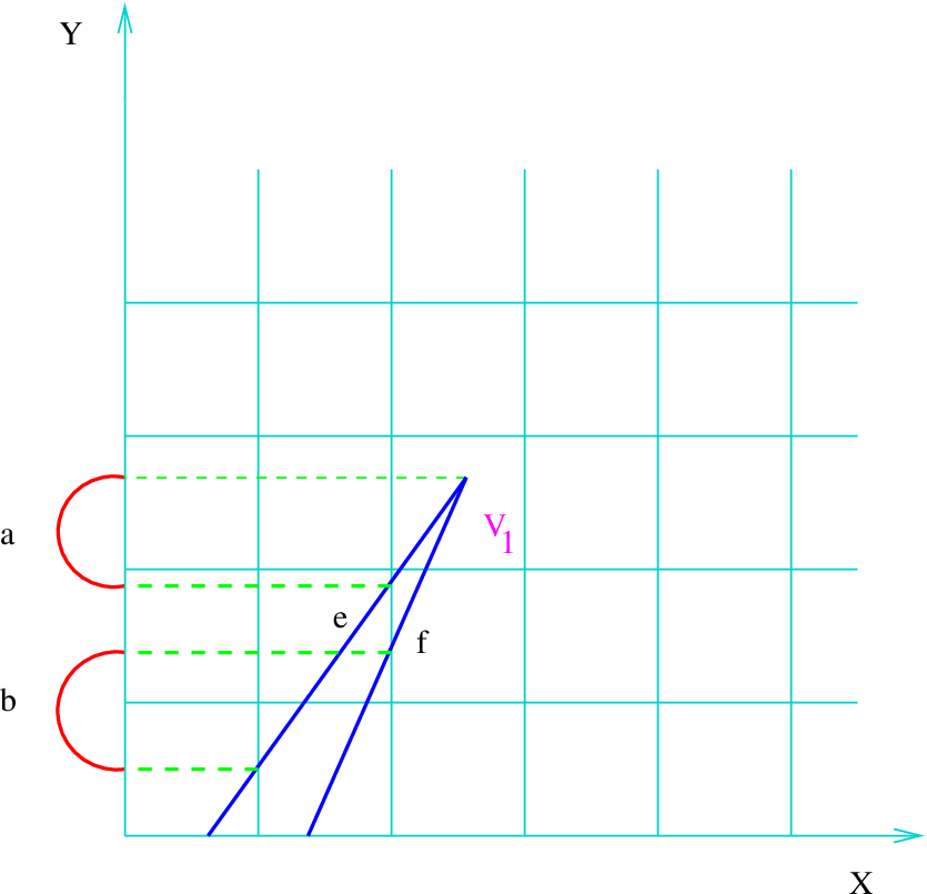
Refer to caption
Figure 13: The second example in two dimensions

In this case we would have tei​ejy=tei​ejy1+tei​ejy2t^{y}_{e_{i}e_{j}}=t^{y_{1}}_{e_{i}e_{j}}+t^{y_{2}}_{e_{i}e_{j}}.

Since in analysing the expectation value for the volume operator we will be considering graphs formed by regular 4-, 6- and 8-valent lattice, it turns out that the angles θi\theta_{i}—the angle formed by the projection on the edge on the xx–yy-plane and the xx-axis—and the angle, ϕi\phi_{i}, with respect to the zz-axis for any edge, are such that two or more edges can only commonly intersect at most one plaquette in a given direction.

When generalising the procedure described above for calculating the values of tei​ejtei​tej\frac{t_{e_{i}e_{j}}}{\sqrt{t_{e_{i}}t_{e_{j}}}} to the 3-dimensional case, some extra care is needed. In fact, consider Figure 14.

Refer to caption
Figure 14: Example in three dimensions

It is clear that the values for teizt^{z}_{e_{i}} can be computed with respect to both the xx- and the yy-coordinates as follows

xtzei=a×cotϕ1cos⁡θ=a×Zxeiytzei=c×cotϕ1sin⁡θ=c×Zyei^{x}t^{z}_{e_{i}}=a\times\cot\phi\frac{1}{\cos\theta}=a\times Z^{x}_{e_{i}}\hskip 36.135pt{}^{y}t^{z}_{e_{i}}=c\times\cot\phi\frac{1}{\sin\theta}=c\times Z^{y}_{e_{i}} (3.4)

where

a={xVj−nxVj​liff the edge points in the negative x directionnxVj​l+l−xVjiff the edge points in the positive x directiona=\begin{cases}x_{V_{j}}-n_{x_{V_{j}}}l&\text{iff the edge points in the negative x direction}\\ n_{x_{V_{j}}}l+l-x_{V_{j}}&\text{iff the edge points in the positive x direction}\end{cases}

and

c={yVj−nyVj​liff the edge points in the negative y directionnyVj​l+l−yVjiff the edge points in the positive y directionc=\begin{cases}y_{V_{j}}-n_{y_{V_{j}}}l&\text{iff the edge points in the negative y direction}\\ n_{y_{V_{j}}}l+l-y_{V_{j}}&\text{iff the edge points in the positive y direction}\end{cases}

The term teizx{}^{x}t^{z}_{e_{i}} in these equations represents the value of teizt^{z}_{e_{i}} as computed with respect to the xx-coordinate, while teizy{}^{y}t^{z}_{e_{i}} is the value of teizt^{z}_{e_{i}} as computed with respect to the yy-coordinate. The non-uniqueness of the computation of the values teizt^{z}_{e_{i}} implies that there is an extra difficulty in the three-dimensional case. We will illustrate this with the aid of an example.

Refer to caption
Figure 15: Computation for the terms teizt^{z}_{e_{i}} in 3-dimensions

Consider the edge eie_{i} in figure 15. The value of teizt^{z}_{e_{i}} can be computed with respect to both the xx and the yy coordinate, thus obtaining teizx{}^{x}t^{z}_{e_{i}} or teizy{}^{y}t^{z}_{e_{i}} respectively. However, it is clear from the diagram that the intersection of the edge eie_{i} with the stack of plaquettes in the zz direction containing the vertex VjV_{j} is given by teizx{}^{x}t^{z}_{e_{i}}. On the other hand teizy{}^{y}t^{z}_{e_{i}} defines the intersection of the edge eie_{i} with the stacks of plaquettes in the zz direction containing the vertex plus the stack in the zz direction delimited, in the xx direction, by the values n​l+lnl+l and n​l+a​lnl+al.

This example shows that, given the values teizx{}^{x}t^{z}_{e_{i}} and teizy{}^{y}t^{z}_{e_{i}}, the intersection of the edge eie_{i} with the stacks of plaquettes in the zz direction which contain the vertex VjV_{j} is given by the smallest term, i.e., tzei=xtzei∩ytzeit^{z}_{e_{i}}=^{x}t^{z}_{e_{i}}\cap^{y}t^{z}_{e_{i}}. It follows that, given two edges eie_{i} and eje_{j}, in order to find tei,ejz:=teiz∩tejzt^{z}_{e_{i},e_{j}}:=t^{z}_{e_{i}}\cap t^{z}_{e_{j}} we first need to establish whether tzei=xtzeit^{z}_{e_{i}}=^{x}t^{z}_{e_{i}} or tzei=ytzeit^{z}_{e_{i}}=^{y}t^{z}_{e_{i}} and similarly for the edge eje_{j}. Once the value of the terms teizt^{z}_{e_{i}} and tejzt^{z}_{e_{j}} is determined, we can proceed as for the two-dimensional case and identify tei​ejzt^{z}_{e_{i}e_{j}} with the smallest tzt^{z}, i.e. tei,ejz:=teiz∩tejzt^{z}_{e_{i},e_{j}}:=t^{z}_{e_{i}}\cap t^{z}_{e_{j}}.

For intersections in the xx and yy stacks the procedure for computing the values of tei​ejt_{e_{i}e_{j}} is essentially the same. However, the formulae for the values of the individual terms, teikj{}^{j}t^{k}_{e_{i}}, are different. Specifically, for the xx-direction we have:

ztxei=d×tanϕcosθ=d×Fxeiytxei=c×cotθ=c×Txei^{z}t^{x}_{e_{i}}=d\times\tan\phi\cos\theta=d\times F^{x}_{e_{i}}\hskip 36.135pt{}^{y}t^{x}_{e_{i}}=c\times\cot\theta=c\times T^{x}_{e_{i}} (3.5)

where

d={zVj−nzVj​liff the edge points upwardsnzVj​l+l−zVjiff the edge points downwardsd=\begin{cases}z_{V_{j}}-n_{z_{V_{j}}}l&\text{iff the edge points upwards}\\ n_{z_{V_{j}}}l+l-z_{V_{j}}&\text{iff the edge points downwards}\end{cases}

and cc is defined as above. For the yy-direction we have

ztyei=d×tanϕsinθ=d×Fyeixtyei=a×tanθ=a×Tyei^{z}t^{y}_{e_{i}}=d\times\tan\phi\sin\theta=d\times F^{y}_{e_{i}}\hskip 36.135pt{}^{x}t^{y}_{e_{i}}=a\times\tan\theta=a\times T^{y}_{e_{i}} (3.6)

where aa and dd are defined as above.

When computing the values of tei​ejtei​tej\frac{t_{e_{i}e_{j}}}{\sqrt{t_{e_{i}}t_{e_{j}}}} in three dimensions, as for the two-dimensional case we need to compute the values for teit_{e_{i}}, which in this case are simply tei=teix+teiy+teiz=δeicos(90−ϕei)cosθei+δeicos(90−ϕei)sinθei+δeicosϕit_{e_{i}}=t^{x}_{e_{i}}+t^{y}_{e_{i}}+t^{z}_{e_{i}}=\delta_{e_{i}}\cos(90-\phi_{e_{i}})\cos\theta_{e_{i}}+\delta_{e_{i}}\cos(90-\phi_{e_{i}})\sin\theta_{e_{i}}+\delta_{e_{i}}\cos\phi_{i}. The explicit values of the terms tei​ejtei​tej\frac{t_{e_{i}e_{j}}}{\sqrt{t_{e_{i}}t_{e_{j}}}} obtained for the 4-, 6-, and 8-valent graph which satisfies condition (a) above, namely |n​l|≤|xV2|≤|n​l+l6||nl|\leq|x_{V_{2}}|\leq|nl+\frac{l}{6}|, for the 4-valent graph and an equivalent condition for the 6- and 8-valent graphs are given in the Appendix.

Since for all 4-, 6- and 8-valent graphs we are dealing with symmetric lattices, after a certain number of vertices the values for the terms tei​ejtei​tej\frac{t_{e_{i}e_{j}}}{\sqrt{t_{e_{i}}t_{e_{j}}}} will repeat, i.e., there will be a periodicity in the values of the terms tei​ejtei​tej\frac{t_{e_{i}e_{j}}}{\sqrt{t_{e_{i}}t_{e_{j}}}}. Therefore, in computing these values we need only consider those vertices which comprise the periodicity cell, i.e., those vertices for which the values of the term tei​ejtei​tej\frac{t_{e_{i}e_{j}}}{\sqrt{t_{e_{i}}t_{e_{j}}}} cannot be obtained through symmetry arguments. As we will see later, this periodicity is different for graphs of different valency.

We now proceed to compute the expectation value of the volume operator for the 4-, 6- and 8-valent cases, utilising the values of the terms tei​ejtei​tej\frac{t_{e_{i}e_{j}}}{\sqrt{t_{e_{i}}t_{e_{j}}}} given in the Appendix.

3.2 Analysis of the expectation value of the volume operator for a 4-valent graph

In this Section we will compute the expectation value of the volume operator as applied to a 4-valent graph. We will first take into consideration the non-rotated graph. In establishing rotational and translational dependence of the expectation value we will perform both a rotation by arbitrary Euler angles and a translation and, then, recalculate the expectation value. We will see that the contributions that come from the terms tei​ejtei​tej\frac{t_{e_{i}e_{j}}}{\sqrt{t_{e_{i}}t_{e_{j}}}}, which comprise the off-diagonal elements of the matrix A−1\sqrt{A}^{-1}, are not trivial, thereby producing a strong rotational and translational dependence in the expectation value of the volume operator in higher order in lδ\frac{l}{\delta}.

3.2.1 Expectation value of the volume operator for a 4-valent graph

To calculate the expectation value of the volume operator we will consider a 4-valent graph constructed from the simplicial cell complex as discussed in [24]. We choose the vertex V0V_{0} to be V0=(0,0,0)V_{0}=(0,0,0), and the angles ϕe=cos−1⁡(13)\phi_{e}=\cos^{-1}(\frac{1}{\sqrt{3}}) and θe=45∘\theta_{e}=45^{\circ} for all e∈γe\in\gamma such that we obtain the configuration depicted in picture 16.

Refer to caption
Figure 16: General vertex of a 4-valent graph

The periodicity cell for a 4-valent graph contains four vertices, including V0V_{0}. The coordinates of the remaining three vertices are V2=(δ3,δ3,δ3)V_{2}=\big(\frac{\delta}{\sqrt{3}},\frac{\delta}{\sqrt{3}},\frac{\delta}{\sqrt{3}}\big); V8=(δ3,3​δ3,δ3)V_{8}=\big(\frac{\delta}{\sqrt{3}},3\frac{\delta}{\sqrt{3}},\frac{\delta}{\sqrt{3}}\big); V13=(0,2​δ3,2​δ3)V_{13}=\big(0,2\frac{\delta}{\sqrt{3}},2\frac{\delta}{\sqrt{3}}\big).

It follows that the edges e0,1e_{0,1}, e0,2e_{0,2}, e0,3e_{0,3} and e0,4e_{0,4} lie in the octants GG, BB, EE and DD respectively. This implies that the geometric factor for the vertex V0V_{0} will be Gγ,V=2G_{\gamma,V}=\sqrt{2}. Because of the geometry of a regular 4-valent graph, it turns out that all the vertices comprising the periodicity cell, V2V_{2}, V8V_{8} and V13V_{13} will have Gγ,Vi=2G_{\gamma,V_{i}}=\sqrt{2}.

The following table gives the values obtained for the terms tei​ejtei​tej\frac{t_{e_{i}e_{j}}}{\sqrt{t_{e_{i}}t_{e_{j}}}} for the 4-valent graph that satisfies condition (a) as defined in the previous Section, namely |n​l|≤|xV2|≤|n​l+l6||nl|\leq|x_{V_{2}}|\leq|nl+\frac{l}{6}|.

It should be noted that, because of the geometry of the 4-valent graph, the terms Tei{x,y}T^{\{x,y\}}_{e_{i}},Fei{x,y}F^{\{x,y\}}_{e_{i}},Zei{x,y}Z^{\{x,y\}}_{e_{i}} in equations 3.4, 3.5 and 3.6 are all equal to 11 for each edge eie_{i}:

V0V_{0} six terms ​tei​ejtei​tej=0\text{six terms }\frac{t_{e_{i}e_{j}}}{\sqrt{t_{e_{i}}t_{e_{j}}}}=0
V2V_{2} six terms tei​ejtei​tej=(δ3−nl)1δ​3\text{six terms }\frac{t_{e_{i}e_{j}}}{\sqrt{t_{e_{i}}t_{e_{j}}}}=\big(\frac{\delta}{\sqrt{3}}-nl\big)\frac{1}{\delta\sqrt{3}}
V8V_{8} six terms ​tei​ejtei​tej=(δ3−n​l)​1δ​3\text{six terms }\frac{t_{e_{i}e_{j}}}{\sqrt{t_{e_{i}}t_{e_{j}}}}=\big(\frac{\delta}{\sqrt{3}}-nl\big)\frac{1}{\delta\sqrt{3}}
V13V_{13} two terms ​tei​ejtei​tej=(2​δ3−2​n​l)​1δ​3\text{two terms }\frac{t_{e_{i}e_{j}}}{\sqrt{t_{e_{i}}t_{e_{j}}}}=\big(\frac{2\delta}{\sqrt{3}}-2nl\big)\frac{1}{\delta\sqrt{3}}

Here, δ\delta is the length of the edge ee. In order to apply equation (2.20), we first need to determine the values of the term dete,e′e′′(A−1)\det_{e,e^{{}^{\prime}}e^{{}^{\prime\prime}}}(\sqrt{A}^{-1}) for each triplet of linearly-independent edges e,e′,e′′e,e^{{}^{\prime}},e^{{}^{\prime\prime}}. Using the fact that, in first-order approximation, (A)−1=1−12​(A−1)(\sqrt{A})^{-1}=1-\frac{1}{2}(A-1), the explicit expression for (A)−1(\sqrt{A})^{-1} for the 4-valent graph under consideration is

(e0,1e0,2e0,11e0,12e2,7e2,5e2,6e13,9e13,8e13,10e13,11e8,13e8,14e8,15e8,5e0,1100000000000000e0,2010012​α−12​α−12​α00000000e0,11001000000000000e0,12000100000000000e2,70−12​α001−12​α−12​α00000000e2,50−12​α00−12​α1−12​α00000000e2,60−12​α00−12​α−12​α100000000e13,900000001−12​α−12​α−12​α0000e13,80000000−12​α1−12​α−12​α0000e13,100000000−12​α−12​α1−12​α0000e13,110000000−12​α−12​α−12​α10000e8,130000000000010−α0e8,1400000000000010−αe8,1500000000000−α010e8,5000000000000−α01)\left(\begin{array}[]{c|ccccccccccccccc}&e_{0,1}&e_{0,2}&e_{0,11}&e_{0,12}&e_{2,7}&e_{2,5}&e_{2,6}&e_{13,9}&e_{13,8}&e_{13,10}&e_{13,11}&e_{8,13}&e_{8,14}&e_{8,15}&e_{8,5}\\ \hline\cr e_{0,1}&1&0&0&0&0&0&0&0&0&0&0&0&0&0&0\\ e_{0,2}&0&1&0&0&\frac{1}{2}\alpha&-\frac{1}{2}\alpha&-\frac{1}{2}\alpha&0&0&0&0&0&0&0&0\\ e_{0,11}&0&0&1&0&0&0&0&0&0&0&0&0&0&0&0\\ e_{0,12}&0&0&0&1&0&0&0&0&0&0&0&0&0&0&0\\ e_{2,7}&0&-\frac{1}{2}\alpha&0&0&1&-\frac{1}{2}\alpha&-\frac{1}{2}\alpha&0&0&0&0&0&0&0&0\\ e_{2,5}&0&-\frac{1}{2}\alpha&0&0&-\frac{1}{2}\alpha&1&-\frac{1}{2}\alpha&0&0&0&0&0&0&0&0\\ e_{2,6}&0&-\frac{1}{2}\alpha&0&0&-\frac{1}{2}\alpha&-\frac{1}{2}\alpha&1&0&0&0&0&0&0&0&0\\ e_{13,9}&0&0&0&0&0&0&0&1&-\frac{1}{2}\alpha&-\frac{1}{2}\alpha&-\frac{1}{2}\alpha&0&0&0&0\\ e_{13,8}&0&0&0&0&0&0&0&-\frac{1}{2}\alpha&1&-\frac{1}{2}\alpha&-\frac{1}{2}\alpha&0&0&0&0\\ e_{13,10}&0&0&0&0&0&0&0&-\frac{1}{2}\alpha&-\frac{1}{2}\alpha&1&-\frac{1}{2}\alpha&0&0&0&0\\ e_{13,11}&0&0&0&0&0&0&0&-\frac{1}{2}\alpha&-\frac{1}{2}\alpha&-\frac{1}{2}\alpha&1&0&0&0&0\\ e_{8,13}&0&0&0&0&0&0&0&0&0&0&0&1&0&-\alpha&0\\ e_{8,14}&0&0&0&0&0&0&0&0&0&0&0&0&1&0&-\alpha\\ e_{8,15}&0&0&0&0&0&0&0&0&0&0&0&-\alpha&0&1&0\\ e_{8,5}&0&0&0&0&0&0&0&0&0&0&0&0&-\alpha&0&1\\ \end{array}\right)

where α=tei​ejtei​tej=(δ3−n​l)​1δ​3\alpha=\frac{t_{e_{i}e_{j}}}{\sqrt{t_{e_{i}}t_{e_{j}}}}=\big(\frac{\delta}{\sqrt{3}}-nl\big)\frac{1}{\delta\sqrt{3}} and the terms tei​ejt_{e_{i}e_{j}}, teit_{e_{i}} and tejt_{e_{j}} are computed using the techniques defined in the previous Section.

Now that we have an expression for the inverse of the matrix A\sqrt{A} we can compute the expectation value of the volume operator for each of the four vertices in the periodicity cell and, then, sum their contributions.

We start with the vertex V0V_{0}. First consider the sub-matrix of the matrix (A)−1(\sqrt{A})^{-1} formed by all the edges incident at V0V_{0}. This is

(e0,1e0,2e0,11e0,12e0,11000e0,20100e0,110010e0,120001)\left(\begin{array}[]{c|ccccc}&e_{0,1}&e_{0,2}&e_{0,11}&e_{0,12}\\ \hline\cr e_{0,1}&1&0&0&0\\ e_{0,2}&0&1&0&0\\ e_{0,11}&0&0&1&0\\ e_{0,12}&0&0&0&1\\ \end{array}\right)

Because of the geometry of the 4-valent graph, at each vertex there are four triplets of linearly-independent edges. Keeping this in mind and computing the determinant of the matrices formed by each such set of triplets, we obtain the following expression for the expectation value of the volume operator at V0V_{0}:

δ3​18​det(Eja​(u))​|16​|det(∂XSa∂(s,u1,u2))|2|12\delta^{3}\sqrt{\frac{1}{8}}\sqrt{\det\big(E^{a}_{j}(u)\big)}\;\Big|16\big|\det\Big(\frac{\partial X_{S}^{a}}{\partial(s,u^{1},u^{2})}\Big)\big|^{2}\Big|^{\frac{1}{2}} (3.7)

By a similar procedure for vertices V2V_{2} and V3V_{3} we obtain

δ3​18​det(Eja​(u))​|16​(1−3​α24−α34)​|det(∂XSa∂(s,u1,u2))|2|12\delta^{3}\sqrt{\frac{1}{8}}\sqrt{\det\big(E^{a}_{j}(u)\big)}\;\Big|16\Big(1-\frac{3\alpha^{2}}{4}-\frac{\alpha^{3}}{4}\Big)\,\big|\det\Big(\frac{\partial X_{S}^{a}}{\partial(s,u^{1},u^{2})}\Big)\big|^{2}\Big|^{\frac{1}{2}} (3.8)

In both cases, the sub-matrix of A−1\sqrt{A}^{-1} we consider is

(1−12​α−12​α−12​α−12​α1−12​α−12​α−12​α−12​α1−12​α−12​α−12​α−12​α1)\left(\begin{array}[]{cccc}1&-\frac{1}{2}\alpha&-\frac{1}{2}\alpha&-\frac{1}{2}\alpha\\ -\frac{1}{2}\alpha&1&-\frac{1}{2}\alpha&-\frac{1}{2}\alpha\\ -\frac{1}{2}\alpha&-\frac{1}{2}\alpha&1&-\frac{1}{2}\alpha\\ -\frac{1}{2}\alpha&-\frac{1}{2}\alpha&-\frac{1}{2}\alpha&1\\ \end{array}\right)

and then we compute the determinant of all the sub-matrices formed by linearly-independent triplets of edges.

For the vertex V4V_{4} we obtain

δ3​18​det(Eja​(u))​|16​(1−α2)​|det(∂XSa∂(s,u1,u2))|2|12\delta^{3}\sqrt{\frac{1}{8}}\sqrt{\det(E^{a}_{j}(u)\big)}\;\Big|16(1-\alpha^{2})\Big|\det\Big(\frac{\partial X_{S}^{a}}{\partial(s,u^{1},u^{2})}\Big)\Big|^{2}\Big|^{\frac{1}{2}} (3.9)

where we have used the sub-matrix

(10−α0010−α−α0100−α01)\left(\begin{array}[]{cccc}1&0&-\alpha&0\\ 0&1&0&-\alpha\\ -\alpha&0&1&0\\ 0&-\alpha&0&1\\ \end{array}\right)

Summing up these contributions gives

VR\displaystyle V_{R} =δ3​18​ 4​|det(∂XSa∂(s,u1,u2))||(1​|det(Eja​(u))|+|det(Eja​(u))|​(|1−3​α24−α34|)12CLOSE\displaystyle=\delta^{3}\sqrt{\frac{1}{8}}\;4\;\Big|\det\Big(\frac{\partial X_{S}^{a}}{\partial(s,u^{1},u^{2})}\Big)\Big|\;\;\Big|\Big(1\sqrt{|\det\big(E^{a}_{j}(u)\big)|}+\sqrt{|\det\big(E^{a}_{j}(u)\big)|}\Big(\big|1-\frac{3\alpha^{2}}{4}-\frac{\alpha^{3}}{4}\,\big|\Big)^{\frac{1}{2}}
+|det(Eja​(u))|(||1−3​α24−α34|)12+|det(Eja​(u))|(|1−α2|)12\displaystyle+\sqrt{|\det\big(E^{a}_{j}(u)\big)|}\Big(\big||1-\frac{3\alpha^{2}}{4}-\frac{\alpha^{3}}{4}\,\big|\Big)^{\frac{1}{2}}+\sqrt{|\det\big(E^{a}_{j}(u)\big)|}\Big(\big|1-\alpha^{2}\,\big|\Big)^{\frac{1}{2}} (3.10)

To first-order approximation we obtain

VR\displaystyle V_{R} =δ3​2​2​|det(Eja​(u))|​|det(∂XSa∂(s,u1,u2))|​1−12​(3​α216−α24)+𝒪⁡(3)\displaystyle=\delta^{3}2\sqrt{2}\sqrt{|\det\big(E^{a}_{j}(u)\big)|}\;\Big|\det\Big(\frac{\partial X_{S}^{a}}{\partial(s,u^{1},u^{2})}\Big)\;\;\Big|1-\frac{1}{2}\Big(\frac{3\alpha^{2}}{16}-\frac{\alpha^{2}}{4}\Big)+\mathcal{O}(3) (3.11)

It should be noted that, although the term det(Eja​(u))\det(E^{a}_{j}(u)) is vertex dependent, we can safely assume that, to first-order in l/δl/\delta, the values will be the same for each vertex within each periodicity cell that involves only an order of four vertices. Thus this term can be factored out from the equation. This first-order approximation will be used throughout the rest of this paper. As mentioned previously this is justified since we choose lδ<<1\frac{l}{\delta}<<1. It follows that the terms α2∝l−xδ\alpha^{2}\propto\frac{l-x}{\delta}, which are much smaller than one (see Section 2.2).

The term proportional to α2\alpha^{2} in the equation above represents the l/δl/\delta-correction for the expectation value of the volume operator for a given region RR. As in [24], for a general 4-valent graph, even in the zeroth-order approximation the expectation value for the volume of a given region RR does not coincide with the classical value for the volume of that region. Notably, there is no linear correction in l/δl/\delta!

3.2.2 Expectation value of the volume operator for a rotated 4-valent graph

We now analyse how the results of the calculations above depend on how the graph is embedded in   R3{\mathchoice{\hbox{\hbox to0.0pt{\kern 2.9444pt\vrule height=6.14993pt\hss}\hbox{$\displaystyle\rm R$}}}{\hbox{\hbox to0.0pt{\kern 2.9444pt\vrule height=6.14993pt\hss}\hbox{$\textstyle\rm R$}}}{\hbox{\hbox to0.0pt{\kern 2.32219pt\vrule height=4.30496pt\hss}\hbox{$\scriptstyle\rm R$}}}{\hbox{\hbox to0.0pt{\kern 1.93889pt\vrule height=3.0589pt\hss}\hbox{$\scriptscriptstyle\rm R$}}}}^{3}. Here we will consider rotational invariance; translational invariance is discussed in the following subsection.

To analyse the rotational dependence of the expectation value of the volume operator, we will perform an Euler rotation of the graph with respect to some arbitrary Euler angles β\beta, ψ\psi, α\alpha and then repeat the calculation. The transformation matrix is

R=(cos⁡ϕ​cos⁡ψ−sin⁡ϕ​cos⁡θ​sin⁡ψcos⁡ψ​sin⁡ϕ+cos⁡θ​cos⁡ϕ​sin⁡ψsin⁡ψ​sin⁡θ−sin⁡ψ​cos⁡ϕ−cos⁡θ​sin⁡ϕ​cos⁡ψ−sin⁡ψ​sin⁡ϕ+cos⁡θ​cos⁡ϕ​sin⁡ψcos⁡ψ​sin⁡θsin⁡θ​sin⁡ϕ−sin⁡θ​cos⁡ϕcos⁡θ)R=\left(\begin{array}[]{ccc}\cos\phi\cos\psi-\sin\phi\cos\theta\sin\psi&\cos\psi\sin\phi+\cos\theta\cos\phi\sin\psi&\sin\psi\sin\theta\\ -\sin\psi\cos\phi-\cos\theta\sin\phi\cos\psi&-\sin\psi\sin\phi+\cos\theta\cos\phi\sin\psi&\cos\psi\sin\theta\\ \sin\theta\sin\phi&-\sin\theta\cos\phi&\cos\theta\end{array}\right)

The coordinates of the rotated vertices are then given by Vi′=R⋅Vi→V^{\prime}_{i}=R\cdot\vec{V_{i}}

(xVi′yVi′zVi′)=(R11​xvi+R12​yvi+R13​zviR21​xvi+R22​yvi+R23​zviR31​xvi+R32​yvi+R33​zvi)\left(\begin{array}[]{c}x_{V^{\prime}_{i}}\\ y_{V^{\prime}_{i}}\\ z_{V^{\prime}_{i}}\end{array}\right)=\left(\begin{array}[]{c}R_{11}x_{v_{i}}+R_{12}y_{v_{i}}+R_{13}z_{v_{i}}\\ R_{21}x_{v_{i}}+R_{22}y_{v_{i}}+R_{23}z_{v_{i}}\\ R_{31}x_{v_{i}}+R_{32}y_{v_{i}}+R_{33}z_{v_{i}}\end{array}\right)

Applying this transformation matrix to the 4-valent graph we obtain the following new coordinates for the vertices:

V2′\displaystyle V^{\prime}_{2} =\displaystyle= ((−R11+R12+R13)​δ3,(−R21+R22+R23)​δ3,(−R31+R32+R33)​δ3)\displaystyle\Big((-R_{11}+R_{12}+R_{13})\frac{\delta}{\sqrt{3}},(-R_{21}+R_{22}+R_{23})\frac{\delta}{\sqrt{3}},(-R_{31}+R_{32}+R_{33})\frac{\delta}{\sqrt{3}}\Big) (3.12)
V8′\displaystyle V^{\prime}_{8} =\displaystyle= ((R11+3​R12+R13)​δ3,(R21+3​R22+R23)​δ3,(R31+3​R32+R33)​δ3)\displaystyle\Big((R_{11}+3R_{12}+R_{13})\frac{\delta}{\sqrt{3}},(R_{21}+3R_{22}+R_{23})\frac{\delta}{\sqrt{3}},(R_{31}+3R_{32}+R_{33})\frac{\delta}{\sqrt{3}}\Big) (3.13)
V13′\displaystyle V^{\prime}_{13} =\displaystyle= (2​(R12−R13)​δ3,2​(R22−R23)​δ3,2​(R32−R33)​δ3)\displaystyle\Big(2(R_{12}-R_{13})\frac{\delta}{\sqrt{3}},2(R_{22}-R_{23})\frac{\delta}{\sqrt{3}},2(R_{32}-R_{33})\frac{\delta}{\sqrt{3}}\Big) (3.14)

The new angles between the rotated edges and the xx,yy,zz-axes can now easily be computed using elementary trigonometry.

As an explanatory example let us consider the edge e0,2e_{0,2}. To find the angles this edge has with respect to the axes we need first to compute the coordinates of the vector e0,2→\vec{e_{0,2}} starting at vertex V0V_{0} and ending at vertex V2V_{2}. In this case, the coordinates of e0,2→\vec{e_{0,2}} coincide with the coordinates of the vertex V2V_{2}:

e2,0→=((−​R11+R12+R13)​δ3,(−​R21+R22+R23)​δ3,(−​R31+R32+R33)​δ3)\vec{e_{2,0}}=\Big((−R_{11}+R_{12}+R_{13})\frac{\delta}{\sqrt{3}},(−R_{21}+R_{22}+R_{23})\frac{\delta}{\sqrt{3}},(−R_{31}+R_{32}+R_{33})\frac{\delta}{\sqrt{3}}\Big) (3.15)

If instead we considered the edge e25e_{25} we would get

e25→=e02−e05=(−(R11+R12+R13)​δ3,−(R21+R22+R23)​δ3,−(R31+R32+R33)​δ3)\vec{e_{25}}=e_{02}-e_{05}=\Big(-(R_{11}+R_{12}+R_{13})\frac{\delta}{\sqrt{3}},-(R_{21}+R_{22}+R_{23})\frac{\delta}{\sqrt{3}},-(R_{31}+R_{32}+R_{33})\frac{\delta}{\sqrt{3}}\Big) (3.16)

Once we have the coordinates for e2,0→\vec{e_{2,0}}, the angle, ϕe2,0\phi_{e_{2,0}}, it forms with respect to the zz-coordinate is

ϕe2,0=tan−1⁡(x2+y2z)=tan−1⁡((−R11+R12+R13)2+(−R21+R22+R23)2(−R31+R32+R33))\phi_{e_{2,0}}=\tan^{-1}\Big(\frac{\sqrt{x^{2}+y^{2}}}{z}\Big)=\tan^{-1}\Big(\frac{\sqrt{(-R_{11}+R_{12}+R_{13})^{2}+(-R_{21}+R_{22}+R_{23})^{2}}}{(-R_{31}+R_{32}+R_{33})}\Big) (3.17)

The angle, θe2,0\theta_{e_{2,0}}, between the projection of the vector on the xx–yy plane and the xx-axis is given by

θe2,0=tan−1⁡(yx)=tan−1⁡(−R21+R22+R23−R11+R12+R13)\theta_{e_{2,0}}=\tan^{-1}\Big(\frac{y}{x}\Big)=\tan^{-1}\left(\frac{-R_{21}+R_{22}+R_{23}}{-R_{11}+R_{12}+R_{13}}\right) (3.18)

In the same way we can obtain the angles for all the edges in our graph in terms of the elements of the transformation matrix. Thus the orientation of each of the edges of the graph will depend on the matrix elements of the transformation matrix, i.e., on the Euler angles that parameterise the rotation.

In order to determine the rotational dependence of the expectation value of the volume operator, we have performed a case study in which the expectation values were computed for all possible orientations of the graphs that have non-zero measure in S​O​(3)SO(3). Such possible orientations were described in Section 2.4. To aid calculational simplicity, these sub-cases are defined in terms of possible ranges of values for the angles θ\theta and ϕ\phi for each edge in the graph, rather than on possible values for the Euler angles.

In order to keep our results as general as possible, we performed our subdivisions so as to cover all possible situations. This is less tedious than it might seem since we are dealing with regular lattices and, therefore, once the angles for the edges of one vertex are fixed, we immediately know the orientation of the edges of all other vertices.

Let us choose V0′V^{\prime}_{0} as our reference vertex with respect to which the possible orientations of the edges are defined. The edges incident at V0′V^{\prime}_{0} are e0,1e_{0,1} , e0,2e_{0,2} , e0,3e_{0,3} , e0,4e_{0,4}. In defining the orientation we use the convention that both 0<ϕ<2​π0<\phi<2\pi and 0<θ<2​π0<\theta<2\pi increases anti-clockwise.

Once the rotational matrix has been applied, whatever the values of the Euler angles might be, we will end up in a situation in which two edges eie_{i}, eje_{j} point upwards, i.e., −π2<ϕei,ϕej<π2-\frac{\pi}{2}<\phi_{e_{i}},\phi_{e_{j}}<\frac{\pi}{2}, and the remaining two edges point downwards, i.e. π2<ϕek,ϕel<3​π2\frac{\pi}{2}<\phi_{e_{k}},\phi_{e_{l}}<\frac{3\pi}{2}. This is a consequence of the geometry of the 4-valent graph. We will call two edges pointing in the same up, or down, direction an ‘up’, or ‘down’, couple respectively. Since we are considering only those edge orientation with measure non-zero in S​O​(3)SO(3), the angles of the edges eie_{i}, eje_{j} of each up/down couple will satisfy the following conditions: |θei|=|90+θej||\theta_{e_{i}}|=|90+\theta_{e_{j}}| and |ϕei|=|ϕej−54.75||\phi_{e_{i}}|=|\phi_{e_{j}}-54.75|

Given a particular choice of up and down couple we have to specify in which octant (see Figure 4) each edge lies. This is required since different octants induce different values for the geometric factor Gγ,VG_{\gamma,V}. The angles θei\theta_{e_{i}} and ϕei\phi_{e_{i}} required for an edge eie_{i} to lie in each of the octants are listed in Table 1 where, again, we use the convention that 0<ϕei<2​π0<\phi_{e_{i}}<2\pi and 0<θei<2​π0<\theta_{e_{i}}<2\pi, with both angles increasing in an anticlockwise direction.

A B C D
ϕei\phi_{e_{i}} 3​π2<ϕei<2​π\frac{3\pi}{2}<\phi_{e_{i}}<2\pi 0<ϕei<π20<\phi_{e_{i}}<\frac{\pi}{2} 0<ϕei<π20<\phi_{e_{i}}<\frac{\pi}{2} 3​π2<ϕei<2​π\frac{3\pi}{2}<\phi_{e_{i}}<2\pi
θei\theta_{e_{i}} 0<θei<π20<\theta_{e_{i}}<\frac{\pi}{2} π2<θei<π\frac{\pi}{2}<\theta_{e_{i}}<\pi π<θei<3​π2\pi<\theta_{e_{i}}<\frac{3\pi}{2} 3​π2<θei<2​π\frac{3\pi}{2}<\theta_{e_{i}}<2\pi
E F G H
ϕei\phi_{e_{i}} π<ϕei<3​π2\pi<\phi_{e_{i}}<\frac{3\pi}{2} π2<ϕei<π\frac{\pi}{2}<\phi_{e_{i}}<\pi π2<ϕei<π\frac{\pi}{2}<\phi_{e_{i}}<\pi π<ϕei<3​π2\pi<\phi_{e_{i}}<\frac{3\pi}{2}
θei\theta_{e_{i}} 0<θei<π20<\theta_{e_{i}}<\frac{\pi}{2} π2<θei<π\frac{\pi}{2}<\theta_{e_{i}}<\pi π<θei<3​π2\pi<\theta_{e_{i}}<\frac{3\pi}{2} 3​π2<θei<2​π\frac{3\pi}{2}<\theta_{e_{i}}<2\pi
Table 1: Angle-ranges for each octant

However, because of the geometry of a 4-valent graph, the allowed angle-ranges have to be restricted to those listed in Table 2.

A B C D
ϕei\phi_{e_{i}} 3​π2<ϕei<2​π−sin−1⁡(13CLOSE\frac{3\pi}{2}<\phi_{e_{i}}<2\pi-\sin^{-1}(\frac{1}{3} sin−1⁡(13<ϕei<π2CLOSE\sin^{-1}(\frac{1}{3}<\phi_{e_{i}}<\frac{\pi}{2} sin−1⁡(13<ϕei<π2CLOSE\sin^{-1}(\frac{1}{3}<\phi_{e_{i}}<\frac{\pi}{2} 3​π2<ϕei<2​π−sin−1⁡(13CLOSE\frac{3\pi}{2}<\phi_{e_{i}}<2\pi-\sin^{-1}(\frac{1}{3}
θei\theta_{e_{i}} 0<θei<π20<\theta_{e_{i}}<\frac{\pi}{2} π2<θei<π\frac{\pi}{2}<\theta_{e_{i}}<\pi π<θei<3​π2\pi<\theta_{e_{i}}<\frac{3\pi}{2} 3​π2<θei<2​π\frac{3\pi}{2}<\theta_{e_{i}}<2\pi
E F G H
ϕei\phi_{e_{i}} π+sin−1⁡(13)<ϕei<3​π2\pi+\sin^{-1}(\frac{1}{3})<\phi_{e_{i}}<\frac{3\pi}{2} π2<ϕei<π−sin−1⁡(13)\frac{\pi}{2}<\phi_{e_{i}}<\pi-\sin^{-1}(\frac{1}{3}) π2<ϕei<π−sin−1⁡(13)\frac{\pi}{2}<\phi_{e_{i}}<\pi-\sin^{-1}(\frac{1}{3}) π+sin−1⁡(13<ϕei<3​π2CLOSE\pi+\sin^{-1}(\frac{1}{3}<\phi_{e_{i}}<\frac{3\pi}{2}
θei\theta_{e_{i}} 0<θei<π20<\theta_{e_{i}}<\frac{\pi}{2} π2<θei<π\frac{\pi}{2}<\theta_{e_{i}}<\pi π<θei<3​π2\pi<\theta_{e_{i}}<\frac{3\pi}{2} 3​π2<θei<2​π\frac{3\pi}{2}<\theta_{e_{i}}<2\pi
Table 2: 4-valent graph angle-ranges for each octant

Our calculations show that for all possible sub-cases of angle arrangements defined in Table 2, the expectation value for the volume operator is rotational invariant only at the zeroth-order99 9 This is a consequence of the fact that the geometric factors Gγ,ViG_{\gamma,V_{i}} for each of the sub-cases in Table 2 will be the same (see Section 2.4.1), while higher-order terms are rotationally dependent. Therefore, in what follows, we will not compute the expectation value for the volume operator as computed for each possible orientation of the graph. Instead we will choose a particular sub-case of Table 2 and compute the expectation value for such a sub-case. Specifically we will choose the case in which the arrangement of edges, incident at the vertex V0V_{0}, after a rotation, is given by the following ranges:

0<θe0,2<π23​π2<ϕe0,2<2​π−sin−1⁡13\displaystyle 0<\theta_{e_{0,2}}<\frac{\pi}{2}\hskip 36.135pt\frac{3\pi}{2}<\phi_{e_{0,2}}<2\pi-\sin^{-1}\frac{1}{3}
π<θe0,4<3​π2sin−1⁡(13)<ϕe0,4<π2\displaystyle\pi<\theta_{e_{0,4}}<\frac{3\pi}{2}\hskip 36.135pt\sin^{-1}(\frac{1}{3})<\phi_{e_{0,4}}<\frac{\pi}{2}
π2<θe0,1<π3​π2<ϕe0,1<π−sin−1⁡(13)\displaystyle\frac{\pi}{2}<\theta_{e_{0,1}}<\pi\hskip 36.135pt\frac{3\pi}{2}<\phi_{e_{0,1}}<\pi-\sin^{-1}(\frac{1}{3})
3​π2<θe0,3<2​ππ+sin−1⁡(13)<ϕe0,3<3​π2\displaystyle\frac{3\pi}{2}<\theta_{e_{0,3}}<2\pi\hskip 36.135pt\pi+\sin^{-1}(\frac{1}{3})<\phi_{e_{0,3}}<\frac{3\pi}{2} (3.19)

This implies that the edges e0,2e_{0,2}, e0,3e_{0,3}, e0,4e_{0,4} and e0,1e_{0,1} lie in the octants AA, HH, CC and FF. From the geometry of the 4-valent lattice, the angles of the edges incident at all the other vertices follow.

There is a vast range of Euler angles for which the case above is obtained but, for the sake of brevity, we will not list them here. What is important, though, is that such case has a non-zero measure in S​O​(3)SO(3).

It should be noted that different combinations of angles within the angle ranges in (3.19) lead to different outcomes for the expectation value of the volume operator, since they lead to different values of the terms tei​ejtei​tej\frac{t_{e_{i}e_{j}}}{\sqrt{t_{e_{i}}t_{e_{j}}}}. However, in zeroth-order, the expectation value of the volume operator will be the same irrespectively of which angles satisfying (3.19) we decide to utilise. In fact, the rotational dependence of the expectation value of the volume operator, in the zeroth-order in lδ\frac{l}{\delta}, is determined solely by the geometric factors Gγ,ViG_{\gamma,V_{i}}. For the case which we are analysing (3.19), the values of Gγ,ViG_{\gamma,V_{i}} will be the same irrespectively of which sub-case of (3.19) we analyse. On the other hand, the dependence of the expectation value of the volume operator on higher orders of lδ\frac{l}{\delta} is determined by the terms tei​ejtei​tej\frac{t_{e_{i}e_{j}}}{\sqrt{t_{e_{i}}t_{e_{j}}}} and, therefore, will depend on the sub-cases we analyse.

This discussion shows that for higher orders in lδ\frac{l}{\delta} the expectation value of the volume operator is rotational dependent since, as stated above, for differing angle-ranges that lead to the same geometric factors, the values of the terms tei​ejtei​tej\frac{t_{e_{i}e_{j}}}{\sqrt{t_{e_{i}}t_{e_{j}}}} will differ.

We will now compute the expectation value of the volume operator for the periodicity cell in the 4-valent graph for the case in which the angles of the edges incident at vertex V0V_{0} satisfy condition (3.19). The first step in order to compute the expectation value of the volume operator is to define the matrix A−1\sqrt{A}^{-1}, whose off-diagonal entries are the terms tei​ejtei​tej\frac{t_{e_{i}e_{j}}}{\sqrt{t_{e_{i}}t_{e_{j}}}}. This matrix is given in Table A.1.1 in the Appendix. Although different combinations of angles satisfying condition (3.19) will lead to different values of the terms tei​ejtei​tej\frac{t_{e_{i}e_{j}}}{\sqrt{t_{e_{i}}t_{e_{j}}}}, however, any such combination will lead to the same non-zero entries of the matrix A−1\sqrt{A}^{-1}. This means that the pairs of edges commonly intersecting a plaquette in a given direction will coincide for any combination of angles satisfying conditions (3.19), even though the number tei,ejt_{e_{i},e_{j}} of plaquettes they commonly intersect will differ in each case. Therefore in computing the matrix A−1\sqrt{A}^{-1} we will not determine the precise value of the individual entries, but we will leave them as general as possible. Their precise values can be computed once a specific combination of angles satisfying (3.19) is chosen.

Given the matrix A−1\sqrt{A}^{-1} we are then able to apply formula (2.33) for computing the expectation value of the volume operator. As in the aligned case, we first compute the expectation value of the volume operator for each of the four vertices, and then sum their contributions. In what follows, the term tei,ejtei​tej\frac{t_{e_{i},e_{j}}}{\sqrt{t_{e_{i}}t_{e_{j}}}} is denoted by αei,ej=tei,ejtei​tej\alpha_{e_{i},e_{j}}=\frac{t_{e_{i},e_{j}}}{\sqrt{t_{e_{i}}t_{e_{j}}}}. An explicit form for these terms can be found in Section 11.1 of the Appendix.

The expectation value for the volume operator for the entire periodicity cell, up to first-order in lδ\frac{l}{\delta} is:

VR=\displaystyle V_{R}= δ3​18​|det(∂XSa∂(s,u1,u2))|​(4​|d​e​t​(Eja​(u))|CLOSE\displaystyle\delta^{3}\sqrt{\frac{1}{8}}\Big|\det\Big(\frac{\partial X_{S}^{a}}{\partial(s,u^{1},u^{2})}\Big)\Big|\Big(4\sqrt{|det\big(E^{a}_{j}(u)\big)|}
+4​|1+12​(−αe8,10,e8,112−αe8,10,e8,122−αe8,10,e8,52−αe8,11,e8,122−αe8,11,e8,52−αe8,12,e8,52)|​|d​e​t​(Eja​(u))|\displaystyle+4\sqrt{|1+\frac{1}{2}(-\alpha_{e_{8,10},e_{8,11}}^{2}-\alpha_{e_{8,10},e_{8,12}}^{2}-\alpha_{e_{8,10},e_{8,5}}^{2}-\alpha_{e_{8,11},e_{8,12}}^{2}-\alpha_{e_{8,11},e_{8,5}}^{2}-\alpha_{e_{8,12},e_{8,5}}^{2})|}\sqrt{|det\big(E^{a}_{j}(u)\big)|}
+4​|1+12​(−αe13,18,e13,152−αe13,19,e13,152−αe13,19,e13,182−αe13,3,e13,152−αe13,3,e13,182−αe13,3,e13,192)|​|d​e​t​(Eja​(u))|\displaystyle+4\sqrt{|1+\frac{1}{2}(-\alpha_{e_{13,18},e_{13,15}}^{2}-\alpha_{e_{13,19},e_{13,15}}^{2}-\alpha_{e_{13,19},e_{13,18}}^{2}-\alpha_{e_{13,3},e_{13,15}}^{2}-\alpha_{e_{13,3},e_{13,18}}^{2}-\alpha_{e_{13,3},e_{13,19}}^{2})|}\sqrt{|det\big(E^{a}_{j}(u)\big)|}
OPEN+4​|1+12​(−αe2,0,e2,52−αe2,0,e2,62−αe2,0,e2,72−αe2,5,e2,62−αe2,5,e2,72−αe2,6,e2,72)|​|d​e​t​(Eja​(u))|)+𝒪⁡(3)\displaystyle+4\sqrt{|1+\frac{1}{2}(-\alpha_{e_{2,0},e_{2,5}}^{2}-\alpha_{e_{2,0},e_{2,6}}^{2}-\alpha_{e_{2,0},e_{2,7}}^{2}-\alpha_{e_{2,5},e_{2,6}}^{2}-\alpha_{e_{2,5},e_{2,7}}^{2}-\alpha_{e_{2,6},e_{2,7}}^{2})|}\sqrt{|det\big(E^{a}_{j}(u)\big)|}\;\Big)+\mathcal{O}(3) (3.20)

By performing a Taylor expansion for each of the roots present in the above formula, we can factor out the term |det(Eja​(u))|\sqrt{|\det\big(E^{a}_{j}(u)\big)|} since, in the first-order approximation that we are considering, they turn out to be the same for each vertex. Such an approximation is justified by the analysis performed in Section (2.2). We then obtain

VR=\displaystyle V_{R}= δ3​2​2​|det(Eja​(u))|​(1+14​(−αe8,10,e8,112−αe8,10,e8,122−αe8,10,e8,52−αe8,11,e8,122−αe8,11,e8,52−αe8,12,e8,52−CLOSECLOSE\displaystyle\delta^{3}2\sqrt{2}\sqrt{|\det\big(E^{a}_{j}(u)\big)|}\Big(1+\frac{1}{4}(-\alpha_{e_{8,10},e_{8,11}}^{2}-\alpha_{e_{8,10},e_{8,12}}^{2}-\alpha_{e_{8,10},e_{8,5}}^{2}-\alpha_{e_{8,11},e_{8,12}}^{2}-\alpha_{e_{8,11},e_{8,5}}^{2}-\alpha_{e_{8,12},e_{8,5}}^{2}-
−αe13,18,e13,152−αe13,19,e13,152−αe13,19,e13,182−αe13,3,e13,152−αe13,3,e13,182−αe13,3,e13,192−\displaystyle-\alpha_{e_{13,18},e_{13,15}}^{2}-\alpha_{e_{13,19},e_{13,15}}^{2}-\alpha_{e_{13,19},e_{13,18}}^{2}-\alpha_{e_{13,3},e_{13,15}}^{2}-\alpha_{e_{13,3},e_{13,18}}^{2}-\alpha_{e_{13,3},e_{13,19}}^{2}- (3.21)
OPENOPENαe2,0,e2,52−αe2,0,e2,62−αe2,0,e2,72−αe2,5,e2,62−αe2,5,e2,72−αe2,6,e2,72))\displaystyle\alpha_{e_{2,0},e_{2,5}}^{2}-\alpha_{e_{2,0},e_{2,6}}^{2}-\alpha_{e_{2,0},e_{2,7}}^{2}-\alpha_{e_{2,5},e_{2,6}}^{2}-\alpha_{e_{2,5},e_{2,7}}^{2}-\alpha_{e_{2,6},e_{2,7}}^{2})\Big) (3.22)
=δ3|det(Eja​(u))|22(1+14(−∑i,j=1;j≠n2​(n−1)αj​i2)|det(δ​XSaδ⁡(s,u1,u2))|)\displaystyle=\delta^{3}\sqrt{|\det\big(E^{a}_{j}(u)\big)|}2\sqrt{2}\bigg(1+\frac{1}{4}\big(-\sum^{\frac{n}{2}(n-1)}_{i,j=1;j\neq}\alpha_{ji}^{2}\big)\;\Big|\det\Big(\frac{\delta X_{S}^{a}}{\delta(s,u^{1},u^{2})}\Big)\Big|\bigg) (3.23)

The term 12(−∑i,j=1;j≠n2​(n−1)αj​i2)\frac{1}{2}(-\sum^{\frac{n}{2}(n-1)}_{i,j=1;j\neq}\alpha^{2}_{ji}) represents l/δl/\delta-corrections. Each term αi,j\alpha_{i,j} is proportional to C​l′δC\frac{l^{\prime}}{\delta} for l′<ll^{\prime}<l; CC is a constant that depends on the Euler angles we chose. On the other hand the geometric factors Gγ,ViG_{\gamma,V_{i}} for cases (3.19) coincide with the geometric factors as computed for any of the sub-cases in Table 2, i.e., Gγ,Vi=2​2G_{\gamma,V_{i}}=2\sqrt{2}. This implies that although for such cases the expectation value of the volume operator is rotational invariant in zeroth-order, nonetheless, it does not reproduce the correct semiclassical limit.

For those embeddings whose measure is zero in S​O​(3)SO(3), the geometric factor turns out to be different and, in zeroth-order in l/δl/\delta, leads to a different value of the expectation value of the volume operator as computed for 4-valent graphs.

3.2.3 Expectation value of the volume operator for a translated 4-valent graph

In this Section we will analyse whether the expectation value of the volume operator for the 4-valent graph is translational invariant with respect to the plaquette.

To perform this analysis we consider our original aligned graph and translate it by an arbitrary vector p→=(ϵx,ϵy,ϵz)\vec{p}=(\epsilon_{x},\epsilon_{y},\epsilon_{z}). The new coordinates for the vertices are:

V′′0\displaystyle V^{{}^{\prime\prime}}_{0} =\displaystyle= (ϵx,ϵy,ϵz)​ with ​ϵx>ϵy>ϵz\displaystyle(\epsilon_{x},\epsilon_{y},\epsilon_{z})\mbox{ with }\epsilon_{x}>\epsilon_{y}>\epsilon_{z} (3.24)
V′′2\displaystyle V^{{}^{\prime\prime}}_{2} =\displaystyle= (−δ3+ϵx,ϵy+δ3,ϵz+δ3)\displaystyle\Big(-\frac{\delta}{\sqrt{3}}+\epsilon_{x},\epsilon_{y}+\frac{\delta}{\sqrt{3}},\epsilon_{z}+\frac{\delta}{\sqrt{3}}\Big) (3.25)
V′′8\displaystyle V^{{}^{\prime\prime}}_{8} =\displaystyle= (δ3+ϵx,ϵy+3​δ3,ϵz+δ3)\displaystyle\Big(\frac{\delta}{\sqrt{3}}+\epsilon_{x},\epsilon_{y}+3\frac{\delta}{\sqrt{3}},\epsilon_{z}+\frac{\delta}{\sqrt{3}}\Big) (3.26)
V′′13\displaystyle V^{{}^{\prime\prime}}_{13} =\displaystyle= (ϵx,ϵy+2​δ3,ϵz−2​δ3)\displaystyle\Big(\epsilon_{x},\epsilon_{y}+2\frac{\delta}{\sqrt{3}},\epsilon_{z}-2\frac{\delta}{\sqrt{3}}\Big) (3.27)

Similarly to the analysis for rotational invariance, the computation of the expectation value of the volume operator can be divided into different sub-cases, each of which would lead to different outcomes.

The first division is given by the choice of the signs and the relations between ϵx\epsilon_{x}, ϵy\epsilon_{y} and ϵz\epsilon_{z}, i.e., whether they are positive or negative and whether one coordinate is bigger or equal to another. Each of these cases can be ultimately subdivided into sub-cases depending on the relation between the ratio b=δ3b=\frac{\delta}{\sqrt{3}} and the coordinates of the translational vector.

To carry out our calculations we choose the following:

  1. 1)

    b>ϵx>ϵy>ϵz>0b>\epsilon_{x}>\epsilon_{y}>\epsilon_{z}>0

  2. 2)

    |Vki|−|Vkj|>nki​l−nkj​l​ for all ​|Vki|>|Vkj||V^{i}_{k}|-|V_{k}^{j}|>n^{i}_{k}l-n^{j}_{k}l\mbox{ for all }|V_{k}^{i}|>|V_{k}^{j}|

Altogether, such conditions will allow to determine both the sign of the coordinates for each of the vertices of the translated graph and also the magnitude relation between the coordinates of each vertex.

However, it will transpire that our result is independent of which case we decide to use to perform the calculations. In fact, as we will see, in zeroth-order, the expectation value of the volume operator for a 4-valent graph is translation invariant up to combinations of measure zero in S​O​(3)SO(3). However, for higher orders of approximation this will no longer be true.

As a first step in our calculations we need to specify the allowed positions for each of the translated vertices. Due to the highly symmetrical structure of the 4-valent graph, in order to determine the allowed positions of each vertex, it suffices to find the allowed positions of one reference vertex. We choose such a reference vertex to be V0V_{0}, whose new coordinates are V0=(ϵx,ϵy,ϵz)V_{0}=(\epsilon_{x},\epsilon_{y},\epsilon_{z}).

The number of stacks intersected by the vector that represents vertex V0V_{0} in the xx, yy and zz-directions are, respectively, n=[ϵxl]n=[\frac{\epsilon_{x}}{l}], m=[ϵyl]m=[\frac{\epsilon_{y}}{l}] and p=[ϵzl]p=[\frac{\epsilon_{z}}{l}] (where [][] indicates the Gauss bracket). It follows that the allowed positions for vertex V0V_{0} are given by the following ranges of each coordinate: n​l<ϵx<n​l+lnl<\epsilon_{x}<nl+l, m​l<ϵy<m​l+lml<\epsilon_{y}<ml+l and p​l<ϵx<p​l+lpl<\epsilon_{x}<pl+l.

It turns out that to carry out the calculations for the expectation value of the volume operator we have to restrict the value-range of the coordinates ϵx\epsilon_{x}, ϵy\epsilon_{y} and ϵz\epsilon_{z}. We choose n​l<ϵx<n​l+l6nl<\epsilon_{x}<nl+\frac{l}{6}, m​l<ϵz<m​l+l6ml<\epsilon_{z}<ml+\frac{l}{6} and p​l<ϵz<p​l+l6pl<\epsilon_{z}<pl+\frac{l}{6}

We will now compute the expectation value of the volume operator of the periodicity lattice of the 4-valent graph. We will not give the details of all the calculations involved since they are quite lengthy. However, the method utilised is the same as for the non-translated case, namely, for each of the four vertices comprising the periodicity cell we consider the sub-matrix of A−1\sqrt{A}^{-1} labelled by the four edges intersecting at the vertex. For each of these sub-matrices, call them MM, we compute the determinant of the four 3×33\times 3 sub-matrices of MM defined by the triplets of linearly-independent edges. We then sum up the contributions coming from each of the vertices. Similarly as for the aligned 4-valent graph we have

Tei{x,y}=Fei{x,y}=Zei{x,y}=1∀ei∈γT^{\{x,y\}}_{e_{i}}=F^{\{x,y\}}_{e_{i}}=Z^{\{x,y\}}_{e_{i}}=1\hskip 36.135pt\forall e_{i}\in\gamma (3.28)

The expression for the matrix A−1\sqrt{A}^{-1} is

(1−C02−B02−C0200000000000−C021−C02−B02−A22−C22−A2200000000−B02−C021−C0200000000000−C02−B02−C021000000000000−A22001−A22−C22000000000−C2200−A221−A22000000000−A2200−C22−A2210000000000000001−A132−C132−A13200000000000−A1321−A132−C13200000000000−C132−A1321−A13200000000000−A132−C132−A13210000000000000001−A82−C82−C8200000000000−A821−C82−C8200000000000−C82−C821−A8200000000000−C82−C82−A821)\left(\begin{array}[]{ccccccccccccccc}1&\frac{-C_{0}}{2}&\frac{-B_{0}}{2}&\frac{-C_{0}}{2}&0&0&0&0&0&0&0&0&0&0&0\\ \frac{-C_{0}}{2}&1&\frac{-C_{0}}{2}&\frac{-B_{0}}{2}&\frac{-A_{2}}{2}&\frac{-C_{2}}{2}&\frac{-A_{2}}{2}&0&0&0&0&0&0&0&0\\ \frac{-B_{0}}{2}&\frac{-C_{0}}{2}&1&\frac{-C_{0}}{2}&0&0&0&0&0&0&0&0&0&0&0\\ \frac{-C_{0}}{2}&\frac{-B_{0}}{2}&\frac{-C_{0}}{2}&1&0&0&0&0&0&0&0&0&0&0&0\\ 0&\frac{-A_{2}}{2}&0&0&1&\frac{-A_{2}}{2}&\frac{-C_{2}}{2}&0&0&0&0&0&0&0&0\\ 0&\frac{-C_{2}}{2}&0&0&\frac{-A_{2}}{2}&1&\frac{-A_{2}}{2}&0&0&0&0&0&0&0&0\\ 0&\frac{-A_{2}}{2}&0&0&\frac{-C_{2}}{2}&\frac{-A_{2}}{2}&1&0&0&0&0&0&0&0&0\\ 0&0&0&0&0&0&0&1&\frac{-A_{13}}{2}&\frac{-C_{13}}{2}&\frac{-A_{13}}{2}&0&0&0&0\\ 0&0&0&0&0&0&0&\frac{-A_{13}}{2}&1&\frac{-A_{13}}{2}&\frac{-C_{13}}{2}&0&0&0&0\\ 0&0&0&0&0&0&0&\frac{-C_{13}}{2}&\frac{-A_{13}}{2}&1&\frac{-A_{13}}{2}&0&0&0&0\\ 0&0&0&0&0&0&0&\frac{-A_{13}}{2}&\frac{-C_{13}}{2}&\frac{-A_{13}}{2}&1&0&0&0&0\\ 0&0&0&0&0&0&0&0&0&0&0&1&\frac{-A_{8}}{2}&\frac{-C_{8}}{2}&\frac{-C_{8}}{2}\\ 0&0&0&0&0&0&0&0&0&0&0&\frac{-A_{8}}{2}&1&\frac{-C_{8}}{2}&\frac{-C_{8}}{2}\\ 0&0&0&0&0&0&0&0&0&0&0&\frac{-C_{8}}{2}&\frac{-C_{8}}{2}&1&\frac{-A_{8}}{2}\\ 0&0&0&0&0&0&0&0&0&0&0&\frac{-C_{8}}{2}&\frac{-C_{8}}{2}&\frac{-A_{8}}{2}&1\\ \end{array}\right)

where Ai=(xVi−ni​l)​1δ​3A_{i}=(x_{V_{i}}-n_{i}l)\frac{1}{\delta\sqrt{3}}, Bi=(yVi−mi​l)​1δ​3B_{i}=(y_{V_{i}}-m_{i}l)\frac{1}{\delta\sqrt{3}}, Ci=(zVi−pi​l)​1δ​3C_{i}=(z_{V_{i}}-p_{i}l)\frac{1}{\delta\sqrt{3}}.

Applying the method described above we compute the expectation value for the volume operator for one periodicity cell to be

VR=\displaystyle V_{R}= 18δ3|det(δ​XSaδ⁡(s,u1,u2))|2×\displaystyle\sqrt{\frac{1}{8}}\delta^{3}|\det\Big(\frac{\delta X_{S}^{a}}{\delta(s,u^{1},u^{2})}\Big)\Big|2\times (3.29)
(|det(Eja​(u))|​|4−B02−2​C02−B0​C02|+|det(Eja​(u))|​|4−2​A22−A22​C2−C22|+CLOSE\displaystyle\Bigg(\sqrt{|\det\Big(E^{a}_{j}(u)\Big)|}\sqrt{|4-B_{0}^{2}-2C_{0}^{2}-B_{0}C_{0}^{2}|}+\sqrt{|\det\Big(E^{a}_{j}(u)\Big)|}\sqrt{|4-2A_{2}^{2}-A_{2}^{2}C_{2}-C_{2}^{2}|}+
OPEN|det(Eja​(u))|​|4−2​A132−A132​C13−C132|+|det(Eja​(u))|​|4−A82−2​C82−A8​C82|)\displaystyle\sqrt{|\det\Big(E^{a}_{j}(u)\Big)|}\sqrt{|4-2A_{13}^{2}-A_{13}^{2}C_{13}-C_{13}^{2}|}+\sqrt{|\det\Big(E^{a}_{j}(u)\Big)|}\sqrt{|4-A_{8}^{2}-2C_{8}^{2}-A_{8}C_{8}^{2}|}\Bigg) (3.30)

In first-order approximation we then obtain

VR=\displaystyle V_{R}= 2​18​δ3​|det(Eja​(u))|​(4−18​(B02+2​C02+B0​C02+2​A22+A22​C2+C22+2​A132+A132​C13+C132+CLOSECLOSE\displaystyle 2\sqrt{\frac{1}{8}}\delta^{3}\sqrt{|\det\Big(E^{a}_{j}(u)\Big)|}\Bigg(4-\frac{1}{8}\Big(B_{0}^{2}+2C_{0}^{2}+B_{0}C_{0}^{2}+2A_{2}^{2}+A_{2}^{2}C_{2}+C_{2}^{2}+2A_{13}^{2}+A_{13}^{2}C_{13}+C_{13}^{2}+
A82+2C82+A8C82))+𝒪(4))|det(δ​XSaδ⁡(s,u1,u2))|\displaystyle A_{8}^{2}+2C_{8}^{2}+A_{8}C_{8}^{2}\Big)\Bigg)+\mathcal{O}(4)\Bigg)\Big|\det\Big(\frac{\delta X_{S}^{a}}{\delta(s,u^{1},u^{2})}\Big)\Big|
=\displaystyle= 2​2​δ3​|det(Eja​(u))|​(1−132​(B02+2​C02+2​A22+C22+2​A132+C132+A82+2​C82)+𝒪⁡(3))​|det(δ​XSaδ⁡(s,u1,u2))|\displaystyle 2\sqrt{2}\delta^{3}\sqrt{|\det\Big(E^{a}_{j}(u)\Big)|}\Bigg(1-\frac{1}{32}\Big(B_{0}^{2}+2C_{0}^{2}+2A_{2}^{2}+C_{2}^{2}+2A_{13}^{2}+C_{13}^{2}+A_{8}^{2}+2C_{8}^{2}\Big)+\mathcal{O}(3)\Bigg)\Big|\det\Big(\frac{\delta X_{S}^{a}}{\delta(s,u^{1},u^{2})}\Big)\Big| (3.31)

where in the last equation we have only considered first-order contributions obtained by the usual Taylor series of the square root (see Section 2.2). Thus, we were able to factor out the term det(Eja​(u))\sqrt{\det(E^{a}_{j}(u))}. As it is evident, the corrections of second order in l/δl/\delta are not translationally invariant.

3.3 Analysis of the expectation value of the volume operator for 6-valent graphs

In this Section we will calculate the expectation value of the volume operator for a 6-valent graph. First we consider the non-rotated graph, then we will analyse the rotational and translational dependence of the expectation value by performing a rotation of the graph, followed by a translation of the graph. We will then recalculate the expectation value.

3.3.1 Expectation value of the volume operator for a general 6-valent graph

Similarly as for the 4-valent graph, we will analyse the case for which δl>0\frac{\delta}{l}>0; the motivation for such a choice was given in Section 2.2. For computational simplicity we will position the graph so that the (0,0,0)(0,0,0) coordinates of the graph coincide with the (0,0,0)(0,0,0) coordinates of the plaquette. We also need to align the graph in such a way that each vertex is symmetrical with respect to the axis. Therefore we will choose, for each vertex VkV_{k}, the value ϕek,i=45\phi_{e_{k,i}}=45 for all edges ek,ie_{k,i} incident at VkV_{k} and θek,i=45\theta_{e_{k,i}}=45 for four edges, while the remaining two will have θek,i=0\theta_{e_{k,i}}=0. This edge orientation corresponds to the limiting case (2) described in Section 2.4.1.

As for the diamond lattice, we choose the vertex V2V_{2} as our reference vertex with respect to which we determine the allowed positions of all the remaining vertices of the graph. We also choose the allowed values of the xx-coordinate of V2V_{2} to be n​l<xV2<n​l+l6nl<x_{V_{2}}<nl+\frac{l}{6}, where, in this case, n=[δ​22​l]n=[\frac{\delta\sqrt{2}}{2l}]. Using the same method used in Section 3.1 we can compute all the terms tei​ejtei​tej\frac{t_{e_{i}e_{j}}}{\sqrt{t_{e_{i}}t_{e_{j}}}} for the periodicity cell of the 6-valent graph that contains nine vertices. Given the geometry of the 6-valent graph we have the following values for the term in equations (3.4)–(3.6)

Zei{x,y}\displaystyle Z^{\{x,y\}}_{e_{i}} ={22 iff ​θei≠01 iff ​θei=0Tei{x,y}={22 iff ​θei≠01 iff ​θei=0\displaystyle=\begin{cases}\frac{2}{\sqrt{2}}&\text{ iff }\theta_{e_{i}}\neq 0\\ 1&\text{ iff }\theta_{e_{i}}=0\end{cases}\hskip 36.135ptT^{\{x,y\}}_{e_{i}}=\begin{cases}\frac{\sqrt{2}}{2}&\text{ iff }\theta_{e_{i}}\neq 0\\ 1&\text{ iff }\theta_{e_{i}}=0\end{cases}
Feix\displaystyle F^{x}_{e_{i}} ={1 iff ​θei≠0∞ iff ​θei=0Feix=1∀ei∈γ\displaystyle=\begin{cases}1&\text{ iff }\theta_{e_{i}}\neq 0\\ \infty&\text{ iff }\theta_{e_{i}}=0\end{cases}\hskip 36.135ptF^{x}_{e_{i}}=1\hskip 36.135pt\forall e_{i}\in\gamma (3.32)

The coordinates of the vertices of the periodicity cell are

V0\displaystyle V_{0} =\displaystyle= (0,0,0)\displaystyle(0,0,0)
V2\displaystyle V_{2} =\displaystyle= (δ​22,0,δ​22)\displaystyle\big(\delta\frac{\sqrt{2}}{2},0,\delta\frac{\sqrt{2}}{2}\big)
V3\displaystyle V_{3} =\displaystyle= ((δ​22−(δ​12,−δ​12,2​δ​22)CLOSECLOSE\displaystyle\big((\delta\frac{\sqrt{2}}{2}-(\delta\frac{1}{2},-\delta\frac{1}{2},2\delta\frac{\sqrt{2}}{2}\big)
V4\displaystyle V_{4} =\displaystyle= (2​δ​22,−2​δ​12,2​δ​22)\displaystyle\big(2\delta\frac{\sqrt{2}}{2},-2\delta\frac{1}{2},2\delta\frac{\sqrt{2}}{2}\big)
V5\displaystyle V_{5} =\displaystyle= (0,−2​δ​12,0)\displaystyle\big(0,-2\delta\frac{1}{2},0\big)
V13\displaystyle V_{13} =\displaystyle= (δ​22,−2​δ​12,δ​22)\displaystyle\big(\delta\frac{\sqrt{2}}{2},-2\delta\frac{1}{2},\delta\frac{\sqrt{2}}{2}\big)
V18\displaystyle V_{18} =\displaystyle= (2​δ​22+δ​12,−1​δ​12,δ​22)\displaystyle\big(2\delta\frac{\sqrt{2}}{2}+\delta\frac{1}{2},-1\delta\frac{1}{2},\delta\frac{\sqrt{2}}{2}\big)
V15\displaystyle V_{15} =\displaystyle= (δ​22−δ,−2​δ​12,3​δ​22)\displaystyle\big(\delta\frac{\sqrt{2}}{2}-\delta,-2\delta\frac{1}{2},3\delta\frac{\sqrt{2}}{2}\big)
V14\displaystyle V_{14} =\displaystyle= (δ​22+δ​12,−3​δ​12,0)\displaystyle\big(\delta\frac{\sqrt{2}}{2}+\delta\frac{1}{2},-3\delta\frac{1}{2},0\big)

The values for the terms tei​ejtei​tej\frac{t_{e_{i}e_{j}}}{\sqrt{t_{e_{i}}t_{e_{j}}}} are given in the section A.2.1 of the appendix

The value for the expectation value of the volume operator for one periodicity cell consisting of nine vertices is computed to be

VR=18​δ3​|det(δ​XSaδ⁡(s,u1,u2))|​2​(8​|det(Eja​(u))|+|8−α22−23(α′)24−α(α′)24−3α(α′)24​22​|det(Eja​(u))|CLOSE\displaystyle V_{R}=\frac{1}{8}\delta^{3}\,\Big|\det\Big(\frac{\delta X_{S}^{a}}{\delta(s,u^{1},u^{2})}\Big)\Big|2\Bigg(\sqrt{8}\sqrt{|\det\Big(E^{a}_{j}(u)\Big)|}+\sqrt{|8-\frac{\alpha^{2}}{2}-\frac{23(\alpha^{{}^{\prime}})^{2}}{4}-\frac{\alpha(\alpha^{{}^{\prime}})^{2}}{4}-\frac{3\alpha(\alpha^{{}^{\prime}})^{2}}{4\sqrt{2}}2}\sqrt{|\det\Big(E^{a}_{j}(u)\Big)|}
+8−5(A3′)22−(A3′)2A34−5​A322−2A32−A3′A3α′2−(α′)2−(A3′)2β4−(A3′)2β2​2−3​β22−2β2−3A3′A3β′2\displaystyle+\sqrt{8-\frac{5(A_{3}^{{}^{\prime}})^{2}}{2}-\frac{(A_{3}^{{}^{\prime}})^{2}A_{3}}{4}-\frac{5A_{3}^{2}}{2}-\sqrt{2}A_{3}^{2}-\frac{A_{3}^{{}^{\prime}}A_{3}\alpha^{{}^{\prime}}}{2}-(\alpha^{{}^{\prime}})^{2}-\frac{(A_{3}^{{}^{\prime}})^{2}\beta}{4}-\frac{(A_{3}^{{}^{\prime}})^{2}\beta}{2\sqrt{2}}-\frac{3\beta^{2}}{2}-\sqrt{2}\beta^{2}-\frac{3A_{3}^{{}^{\prime}}A_{3}\beta^{{}^{\prime}}}{2}}
−2A3′A3β′−α′ββ′2−α′ββ′2​2−7(β′)22−A3(β′)22​2|¯​|det(Eja​(u))|+|8−12​β2−8​2​β2|​|det(Eja​(u))|\displaystyle\overline{-\sqrt{2}A_{3}^{{}^{\prime}}A_{3}\beta^{{}^{\prime}}-\frac{\alpha^{{}^{\prime}}\beta\beta^{{}^{\prime}}}{2}-\frac{\alpha^{{}^{\prime}}\beta\beta^{{}^{\prime}}}{2\sqrt{2}}-\frac{7(\beta^{{}^{\prime}})^{2}}{2}-\frac{A_{3}(\beta^{{}^{\prime}})^{2}}{2\sqrt{2}}|}\sqrt{|\det\Big(E^{a}_{j}(u)\Big)|}+\sqrt{|8-12\beta^{2}-8\sqrt{2}\beta^{2}|}\sqrt{|\det\Big(E^{a}_{j}(u)\Big)|}
+|8−2α2−9(α′)2−22α(α′)2−12β2−82β2−12α′ββ′−92α′ββ′−12(β′)2−4α(β′)2|​|det(Eja​(u))|\displaystyle+\sqrt{|8-2\alpha^{2}-9(\alpha^{{}^{\prime}})^{2}-2\sqrt{2}\alpha(\alpha^{{}^{\prime}})^{2}-12\beta^{2}-8\sqrt{2}\beta^{2}-12\alpha^{{}^{\prime}}\beta\beta^{{}^{\prime}}-9\sqrt{2}\alpha^{{}^{\prime}}\beta\beta^{{}^{\prime}}-12(\beta^{{}^{\prime}})^{2}-4\alpha(\beta^{{}^{\prime}})^{2}|}\sqrt{|\det\Big(E^{a}_{j}(u)\Big)|}
+|8−7​α24−7(α′)22−13α(α′)28​2−2αβ−22αβ−(α′)2β2−3(α′)2β2​2−6β2−5αα′β′2​2−2α′ββ′−4(β′)2|\displaystyle+\sqrt{|8-\frac{7\alpha^{2}}{4}-\frac{7(\alpha^{{}^{\prime}})^{2}}{2}-\frac{13\alpha(\alpha^{{}^{\prime}})^{2}}{8\sqrt{2}}-2\alpha\beta-2\sqrt{2}\alpha\beta-\frac{(\alpha^{{}^{\prime}})^{2}\beta}{2}-\frac{3(\alpha^{{}^{\prime}})^{2}\beta}{2\sqrt{2}}-6\beta^{2}-\frac{5\alpha\alpha^{{}^{\prime}}\beta^{{}^{\prime}}}{2\sqrt{2}}-2\alpha^{{}^{\prime}}\beta\beta^{{}^{\prime}}-4(\beta^{{}^{\prime}})^{2}|}
×|det(Eja​(u))|+|8−3(A′18)22−α2/2−A′18αα′2​2−3(α′)24−3β2−22β2−A′18ββ′−3A′18ββ′2​2−α′ββ′2−\displaystyle\times\sqrt{|\det\Big(E^{a}_{j}(u)\Big)|}+\sqrt{|8-\frac{3(A^{{}^{\prime}}_{18})^{2}}{2}-\alpha^{2}/2-\frac{A^{{}^{\prime}}_{18}\alpha\alpha^{{}^{\prime}}}{2\sqrt{2}}-\frac{3(\alpha^{{}^{\prime}})^{2}}{4}-3\beta^{2}-2\sqrt{2}\beta^{2}-A^{{}^{\prime}}_{18}\beta\beta^{{}^{\prime}}-\frac{3A^{{}^{\prime}}_{18}\beta\beta^{{}^{\prime}}}{2\sqrt{2}}-\frac{\alpha^{{}^{\prime}}\beta\beta^{{}^{\prime}}}{2}-}
−3α′ββ′4​2−3(β′)2−α(β′)22|¯​|det(Eja​(u))|+|8−3(A′15)2−(A′15)2A152−2A152−3A′15A15α′2−9(α′)2\displaystyle\overline{-\frac{3\alpha^{{}^{\prime}}\beta\beta^{{}^{\prime}}}{4\sqrt{2}}-3(\beta^{{}^{\prime}})^{2}-\frac{\alpha(\beta^{{}^{\prime}})^{2}}{2}|}\sqrt{|\det\Big(E^{a}_{j}(u)\Big)|}+\sqrt{|8-3(A^{{}^{\prime}}_{15})^{2}-\frac{(A^{{}^{\prime}}_{15})^{2}A_{15}}{\sqrt{2}}-2A_{15}^{2}-\frac{3A^{{}^{\prime}}_{15}A_{15}\alpha^{{}^{\prime}}}{\sqrt{2}}-9(\alpha^{{}^{\prime}})^{2}}
−9A15(α′)24​2−3(A′15)2β2−(A′15)2β2−32A15β−9(α′)2β2−10β2−42β2−A′15A15β′2−3α′ββ′−32α′ββ′¯\displaystyle\overline{-\frac{9A_{15}(\alpha^{{}^{\prime}})^{2}}{4\sqrt{2}}-\frac{3(A^{{}^{\prime}}_{15})^{2}\beta}{2}-\frac{(A^{{}^{\prime}}_{15})^{2}\beta}{\sqrt{2}}-3\sqrt{2}A_{15}\beta-\frac{9(\alpha^{{}^{\prime}})^{2}\beta}{2}-10\beta^{2}-4\sqrt{2}\beta^{2}-\frac{A^{{}^{\prime}}_{15}A_{15}\beta^{{}^{\prime}}}{\sqrt{2}}-3\alpha^{{}^{\prime}}\beta\beta^{{}^{\prime}}-3\sqrt{2}\alpha^{{}^{\prime}}\beta\beta^{{}^{\prime}}}
−2(β′)2|¯​|det(Eja​(u))|+|8−2(A′14)2−A142−3(A′14)2β4−3(A′14)2β2​2−32A14β\displaystyle\overline{-2(\beta^{{}^{\prime}})^{2}|}\sqrt{|\det\Big(E^{a}_{j}(u)\Big)|}+\sqrt{|8-2(A^{{}^{\prime}}_{14})^{2}-A_{14}^{2}-\frac{3(A^{{}^{\prime}}_{14})^{2}\beta}{4}-\frac{3(A^{{}^{\prime}}_{14})^{2}\beta}{2\sqrt{2}}-3\sqrt{2}A_{14}\beta}
OPEN−18β2−92β2−3A′14A14β′2−9A′14ββ′2−9(β′)2|¯​|det(Eja​(u))|)\displaystyle\overline{-18\beta^{2}-9\sqrt{2}\beta^{2}-\frac{3A^{{}^{\prime}}_{14}A_{14}\beta^{{}^{\prime}}}{\sqrt{2}}-\frac{9A^{{}^{\prime}}_{14}\beta\beta^{{}^{\prime}}}{2}-9(\beta^{{}^{\prime}})^{2}|}\sqrt{|\det\Big(E^{a}_{j}(u)\Big)|}\;\Bigg) (3.33)

Expanding the square root (see the analysis in Section 2.2) and considering first-order terms we obtain

VR=2δ3|det(Eja​(u))||det(δ​XSaδ⁡(s,u1,u2))|(9+12×18(−2(A14′)2−3(A15′)2−3(A′18)22−5(A3′)22−A142\displaystyle V_{R}=2\delta^{3}\sqrt{|\det\big(E^{a}_{j}(u)\big)|}\,\Big|\det\Big(\frac{\delta X_{S}^{a}}{\delta(s,u^{1},u^{2})}\Big)\Big|\Bigg(9+\frac{1}{2}\times\frac{1}{8}\big(-2(A^{{}^{\prime}}_{14})^{2}-3(A^{{}^{\prime}}_{15})^{2}-\frac{3(A^{{}^{\prime}}_{18})^{2}}{2}-\frac{5(A_{3}^{{}^{\prime}})^{2}}{2}-A_{14}^{2}
−2A152−5​A322−2A32−19​α24−29(α′)2−32A14β−32A15β−2αβ−22αβ−125​β22−322β2−67(β′)22))\displaystyle-2A_{15}^{2}-\frac{5A_{3}^{2}}{2}-\sqrt{2}A_{3}^{2}-\frac{19\alpha^{2}}{4}-29(\alpha^{{}^{\prime}})^{2}-3\sqrt{2}A_{14}\beta-3\sqrt{2}A_{15}\beta-2\alpha\beta-2\sqrt{2}\alpha\beta-\frac{125\beta^{2}}{2}-32\sqrt{2}\beta^{2}-\frac{67(\beta^{{}^{\prime}})^{2}}{2})\;\Bigg) (3.34)

Contrary to [24] we find that, to zeroth-order in l/δl/\delta, the expectation value of the volume operator for a 6-valent graph does not have the correct semiclassical limit. On the other hand, if the graph is aligned to the orientation of the plaquette we do obtain the correct semiclassical value. However, this embedding has measure zero in S​O​(3)SO(3).

3.3.2 Expectation value of the volume operator for a rotated 6-valent graph

We will now analyse the expectation value of the volume operator for a rotated 6-valent graph. As for the 4-valent graph, different choices of Euler angles in the rotation give different values of tei​ejt_{e_{i}e_{j}}. Therefore, we will once again have to define sub-cases which are defined according to the possible ranges of values for the angles ϕei\phi_{e_{i}} and θei\theta_{e_{i}} for each edge eie_{i}. Because of the geometry of the 6-valent lattice, we know that for any edge, ee, of a given vertex there exists a co-linear edge, e′e^{\prime}, which intersects the same vertex. This implies that, given two co-linear edges ee and e′e^{\prime}, we can define the angles of ee (respectively e′e^{\prime}) in terms of e′e^{\prime} (respectively ee) as follows: ϕe=180∘−ϕe′\phi_{e}=180^{\circ}-\phi_{e^{\prime}} and θe=180∘−θe′\theta_{e}=180^{\circ}-\theta_{e^{\prime}}. Such relations reduce the number of cases that need to be analysed.

We choose the vertex V0′V^{\prime}_{0} as our reference vertex. The relations for the angles of the edges incident at V0′V^{\prime}_{0} are:

ϕe0,7\displaystyle\phi_{e_{0,7}} =\displaystyle= 180∘−ϕe0,2\displaystyle 180^{\circ}-\phi_{e_{0,2}}
ϕe0,1\displaystyle\phi_{e_{0,1}} =\displaystyle= 180∘−ϕe0,17\displaystyle 180^{\circ}-\phi_{e_{0,17}}
ϕe0,6\displaystyle\phi_{e_{0,6}} =\displaystyle= 180∘−ϕe0,8\displaystyle 180^{\circ}-\phi_{e_{0,8}}
θe0,8\displaystyle\theta_{e_{0,8}} =\displaystyle= 180∘−θe0,6\displaystyle 180^{\circ}-\theta_{e_{0,6}}
θe0,17\displaystyle\theta_{e_{0,17}} =\displaystyle= 180∘−θe0,1\displaystyle 180^{\circ}-\theta_{e_{0,1}}
θe0,2\displaystyle\theta_{e_{0,2}} =\displaystyle= 180∘−θe0,7\displaystyle 180^{\circ}-\theta_{e_{0,7}} (3.35)

These relations imply that the allowed values of the angles of the edges at a given vertex fall into one of the following groups:

  1. 1.

    A given triplet of edges points upwards, i.e., their angle ϕ\phi lies between −π2-\frac{\pi}{2} and π2\frac{\pi}{2}, and the triplet formed by their co-linear edges points downwards, i.e., their angle ϕ\phi lies between π2\frac{\pi}{2} and 3​π2\frac{3\pi}{2}. This situation arises when none of the edges is aligned with one of the xx, yy, zz-coordinates. However we have two distinct sub-cases which satisfy this arrangement of edges

    • a.

      No edge lies in any plaquette.

    • b.

      Only one edge and its co-planar lie in a given plaquette (Figure 3).

  2. 2.

    A given couple of edges points upwards i.e., their angle ϕ\phi lies between −π2-\frac{\pi}{2} and π2\frac{\pi}{2}, and their co-linear edges point downwards i.e., their angle ϕ\phi lies between π2\frac{\pi}{2} and 3​π2\frac{3\pi}{2}. This situation arises when one edge (and subsequently its collinear edge) is aligned with one of the coordinates axis and, subsequently, the remaining two edges and their co-linear lie in two different plaquettes in the same direction (Figure 5)

  3. 3.

    Only one edge points upwards, i.e., its angle ϕ\phi lies between −π2-\frac{\pi}{2} and π2\frac{\pi}{2}, and the co-linear edge points downwards i.e., its angle ϕ\phi lies between π2\frac{\pi}{2} and 3​π2\frac{3\pi}{2}. This situation arises when all of the edges are aligned with the coordinate axis (Figure 6).

A discussion of each of these cases and the respective value for the geometric factor was carried out in Section 2.4.1. There it was shown that only case 1a above has non-zero measure in SO(3), therefore we will restrict our analysis to such a case.

It is straight forward to see that case 1a can be divided into further sub-cases according to the values of the θ\theta-angles and the relations between the ϕ\phi-angles of each of the up/down couples. In what follows, we will not give the results for all possible choices. Instead, we will choose a particular sub-case and perform the calculations for the expectation value of the volume operator with respect to this sub-case. As we will see, these calculations show that, up to embeddings of measure zero in S​O​(3)SO(3), the semiclassical behavior of the volume operator, in zeroth-order, does not depend on how the graph is rotated: a fortiori, it is independent of the particular case we analysed.

In order to carry out a proper comparison between the semiclassical behavior of the volume operator as applied to graphs of different valence, we will apply the same Euler transformations (i.e., with the same Euler angles) to each of the graphs we consider. Since we have not specified the values of the Euler angles, the only way to do this is to assume that after a rotation, those edges which had the same angles used in both the aligned 4-valent and 6-valent case will end up in the same octant. For example, consider Figures 17 and 18 which depict both 6-valent and 4-valent vertices respectively. From such pictures it is easy to see that the edges e0,2e_{0,2} and e0,3e_{0,3} of the 4-valent graph have the same θ\theta- and ϕ\phi-angles as the edges, e0,8e_{0,8}, and, e0,1e_{0,1}, of the 6-valent graph. Therefore, in the rotated case we will assume that e0,8e_{0,8}, and, e0,1e_{0,1} lie in the same octants as e0,2e_{0,2} and e0,3e_{0,3} respectively. It follows that the angle-ranges for the edges incident at vertex V0V_{0} for a 6-valent graph are:

3​π2<θe0,2<7​π43​π2<ϕe0,2<2​π\displaystyle\frac{3\pi}{2}<\theta_{e_{0,2}}<\frac{7\pi}{4}\hskip 36.135pt\frac{3\pi}{2}<\phi_{e_{0,2}}<2\pi
π4<θe0,8<π20<ϕe0,8<π2\displaystyle\frac{\pi}{4}<\theta_{e_{0,8}}<\frac{\pi}{2}\hskip 36.135pt0<\phi_{e_{0,8}}<\frac{\pi}{2}
3​π4<θe0,17<π0<ϕe0,17<π2\displaystyle\frac{3\pi}{4}<\theta_{e_{0,17}}<\pi\hskip 36.135pt0<\phi_{e_{0,17}}<\frac{\pi}{2}
π2<θe0,7<3​π4π2<ϕe0,7<π\displaystyle\frac{\pi}{2}<\theta_{e_{0,7}}<\frac{3\pi}{4}\hskip 36.135pt\frac{\pi}{2}<\phi_{e_{0,7}}<\pi
π2<θe0,6<3​π4π<ϕe0,6<3​π2\displaystyle\frac{\pi}{2}<\theta_{e_{0,6}}<\frac{3\pi}{4}\hskip 36.135pt\pi<\phi_{e_{0,6}}<\frac{3\pi}{2}
7​π4<θe0,1<2​ππ<ϕe0,1<3​π2\displaystyle\frac{7\pi}{4}<\theta_{e_{0,1}}<2\pi\hskip 36.135pt\pi<\phi_{e_{0,1}}<\frac{3\pi}{2} (3.36)

Such conditions of the angles implies that the edges e0,1e_{0,1}, e0,2e_{0,2}, e0,6e_{0,6}, e0,7e_{0,7}, e0,7e_{0,7} and e0,17e_{0,17} lie in the octants HH, DD, GG, FF, AA and BB respectively.

Since we are considering a regular 6-valent lattice, the above ranges of angles induce a relation on all the other angle-ranges of the edges for each vertex in the graph.

Refer to caption
Figure 17: 6-valent vertex
Refer to caption
Figure 18: 4-valent vertex

The coordinates of the rotated vertices are:

V0′\displaystyle V^{\prime}_{0} =\displaystyle= (0,0,0)\displaystyle\Big(0,0,0\Big)
V2′\displaystyle V^{\prime}_{2} =\displaystyle= ((R11+R13)​δ​22,(R21+R23)​δ​22,(R31+2​R33)​δ​22)\displaystyle\Big((R_{11}+R_{13})\frac{\delta\sqrt{2}}{2},(R_{21}+R_{23})\frac{\delta\sqrt{2}}{2},(R_{31}+2R_{33})\frac{\delta\sqrt{2}}{2}\Big)
V3′\displaystyle V^{\prime}_{3} =\displaystyle= ((R11​(2−12)−R122+R13​2)​δ,(R21​(2−12)−R222+R23​2)​δ,(R31​(2−12)−R322+R33​2)​δ)\displaystyle\Big((R_{11}(\frac{\sqrt{2}-1}{2})-\frac{R_{12}}{2}+R_{13}\sqrt{2})\delta,(R_{21}(\frac{\sqrt{2}-1}{2})-\frac{R_{22}}{2}+R_{23}\sqrt{2})\delta,(R_{31}(\frac{\sqrt{2}-1}{2})-\frac{R_{32}}{2}+R_{33}\sqrt{2})\delta\Big)
V4′\displaystyle V_{4}^{\prime} =\displaystyle= ((2​R11−R12+2​R13)​δ,(2​R21−R22+2​R23)​δ,(2​R31−R32+2​R33)​δ)\displaystyle\Big((\sqrt{2}R_{11}-R_{12}+\sqrt{2}R_{13})\delta,(\sqrt{2}R_{21}-R_{22}+\sqrt{2}R_{23})\delta,(\sqrt{2}R_{31}-R_{32}+\sqrt{2}R_{33})\delta\Big)
V5′\displaystyle V_{5}^{\prime} =\displaystyle= (−R12​δ,R22​δ,R32​δ)\displaystyle\Big(-R_{12}\delta,R_{22}\delta,R_{32}\delta\Big)
V13′\displaystyle V_{13}^{\prime} =\displaystyle= ((−22​R11−R12+22​R13)​δ,(−22​R21−R22+22​R23)​δ,(−22​R31−R32+22​R33)​δ)\displaystyle\Big((-\frac{\sqrt{2}}{2}R_{11}-R_{12}+\frac{\sqrt{2}}{2}R_{13})\delta,(-\frac{\sqrt{2}}{2}R_{21}-R_{22}+\frac{\sqrt{2}}{2}R_{23})\delta,(-\frac{\sqrt{2}}{2}R_{31}-R_{32}+\frac{\sqrt{2}}{2}R_{33})\delta\Big)
V18′\displaystyle V_{18}^{\prime} =\displaystyle= (((2+12)​R11−12​R12+22​R13)​δ,((2+12)​R21−12​R22+22​R23)​δ,((2+12)​R31−12​R32+22​R33)​δ)\displaystyle\Big(((\sqrt{2}+\frac{1}{2})R_{11}-\frac{1}{2}R_{12}+\frac{\sqrt{2}}{2}R_{13})\delta,((\sqrt{2}+\frac{1}{2})R_{21}-\frac{1}{2}R_{22}+\frac{\sqrt{2}}{2}R_{23})\delta,((\sqrt{2}+\frac{1}{2})R_{31}-\frac{1}{2}R_{32}+\frac{\sqrt{2}}{2}R_{33})\delta\Big)
V15′\displaystyle V^{\prime}_{15} =\displaystyle= (((22−1)​R11−R12+3​22​R13)​δ,((22−1)​R21−R22+3​22​R23)​δ,((22−1)​R31−R32+3​22​R33)​δ)\displaystyle\Big(((\frac{\sqrt{2}}{2}-1)R_{11}-R_{12}+\frac{3\sqrt{2}}{2}R_{13})\delta,((\frac{\sqrt{2}}{2}-1)R_{21}-R_{22}+\frac{3\sqrt{2}}{2}R_{23})\delta,((\frac{\sqrt{2}}{2}-1)R_{31}-R_{32}+\frac{3\sqrt{2}}{2}R_{33})\delta\Big)
V14′\displaystyle V_{14}^{\prime} =\displaystyle= ((2+12​R11−32​R12)​δ,(2+12​R21−32​R22)​δ,(2+12​R31−32​R32)​δ)\displaystyle\Big((\frac{\sqrt{2}+1}{2}R_{11}-\frac{3}{2}R_{12})\delta,(\frac{\sqrt{2}+1}{2}R_{21}-\frac{3}{2}R_{22})\delta,(\frac{\sqrt{2}+1}{2}R_{31}-\frac{3}{2}R_{32})\delta\Big) (3.37)

Similarly, as was done for the 4-valent case, different choices of combination of angles satisfying conditions (3.36) above will lead to different values for the terms tei,ejtei​tej\frac{t_{e_{i},e_{j}}}{\sqrt{t_{e_{i}}t_{e_{j}}}}. However, the couples of edges commonly intersecting a given stack will coincide for any such combination. This implies that the matrix A−1\sqrt{A}^{-1} will have the same entries for any sub-case of (3.36) but their specific values will be different.

Moreover, the geometric factor Gγ,VG_{\gamma,V} of any sub-case of (3.36) will coincide. It follows that any combination of angles that satisfies conditions (3.36) will lead to the same value in zeroth-order in lδ\frac{l}{\delta} of the expectation value for the volume operator. Therefore, as was done for the 4-valent case, in order to compute the expectation value for the volume operator, we will not specify a particular sub-case of (3.36), but leave the result as general as possible.

Given conditions 3.36 the expectation value of the volume for the periodicity cell is

VR=δ318|det(δ​XSaδ⁡(s,u1,u2))|2{22×|d​e​t​(Eja​(u))|\displaystyle V_{R}=\delta^{3}\sqrt{\frac{1}{8}}\Big|\det\Bigg(\frac{\delta X_{S}^{a}}{\delta(s,u^{1},u^{2})}\bigg)\Big|2\Bigg\{2\sqrt{2}\times\sqrt{|det\Big(E^{a}_{j}(u)\Big)|}
+|8+12(−ρ63,832−ρ63,232−ρ113,632−ρ113,832−ρ113,1332−ρ113,232−ρ173,632−ρ173,832−ρ173,1332−ρ173,232\displaystyle+\sqrt{|8+\frac{1}{2}\Big(-\rho_{6_{3},8_{3}}^{2}-\rho_{6_{3},2_{3}}^{2}-\rho_{11_{3},6_{3}}^{2}-\rho_{11_{3},8_{3}}^{2}-\rho_{11_{3},13_{3}}^{2}-\rho_{11_{3},2_{3}}^{2}-\rho_{17_{3},6_{3}}^{2}-\rho_{17_{3},8_{3}}^{2}-\rho_{17_{3},13_{3}}^{2}-\rho_{17_{3},2_{3}}^{2}}
−ρ133,832−ρ133,232)|¯×|d​e​t​(Eja​(u))|\displaystyle\qquad\overline{-\rho_{13_{3},8_{3}}^{2}-\rho_{13_{3},2_{3}}^{2}\Big)|}\times\sqrt{|det\Big(E^{a}_{j}(u)\Big)|}
+|8+12(−ρ141​3,211​32−ρ91​3,141​32−ρ31​3,211​32−ρ31​3,91​32−ρ41​3,91​32−ρ41​3,211​32−ρ41​3,31​32−ρ41​3,141​32−ρ51​3,91​32\displaystyle+\sqrt{|8+\frac{1}{2}\Big(-\rho_{14_{1}3,21_{1}3}^{2}-\rho_{9_{1}3,14_{1}3}^{2}-\rho_{3_{1}3,21_{1}3}^{2}-\rho_{3_{1}3,9_{1}3}^{2}-\rho_{4_{1}3,9_{1}3}^{2}-\rho_{4_{1}3,21_{1}3}^{2}-\rho_{4_{1}3,3_{1}3}^{2}-\rho_{4_{1}3,14_{1}3}^{2}-\rho_{5_{1}3,9_{1}3}^{2}}
−ρ51​3,211​32−ρ51​3,31​32−ρ51​3,141​32)|¯×|d​e​t​(Eja​(u))|\displaystyle\qquad\overline{-\rho_{5_{1}3,21_{1}3}^{2}-\rho_{5_{1}3,3_{1}3}^{2}-\rho_{5_{1}3,14_{1}3}^{2}\Big)|}\times\sqrt{|det\Big(E^{a}_{j}(u)\Big)|}
+|8+12(−ρ02,1022−ρ02,1122−ρ02,322−ρ02,922−ρ112,322−ρ122,1022−ρ122,1122−ρ122,322−ρ122,922−ρ92,1022\displaystyle+\sqrt{|8+\frac{1}{2}\Big(-\rho_{0_{2},10_{2}}^{2}-\rho_{0_{2},11_{2}}^{2}-\rho_{0_{2},3_{2}}^{2}-\rho_{0_{2},9_{2}}^{2}-\rho_{11_{2},3_{2}}^{2}-\rho_{12_{2},10_{2}}^{2}-\rho_{12_{2},11_{2}}^{2}-\rho_{12_{2},3_{2}}^{2}-\rho_{12_{2},9_{2}}^{2}-\rho_{9_{2},10_{2}}^{2}}
−ρ112,1022−ρ92,322)|¯×|d​e​t​(Eja​(u))|\displaystyle\overline{-\rho_{11_{2},10_{2}}^{2}-\rho_{9_{2},3_{2}}^{2}\Big)|}\times\sqrt{|det\Big(E^{a}_{j}(u)\Big)|}
+|8+12(−ρ121​2,41​22−ρ121​2,f1​22−ρ91​2,121​22−ρ91​2,41​22−ρ91​2,e1​22−ρ91​2,f1​22−ρd1​2,121​22−ρd1​2,41​22−ρd1​2,e1​22\displaystyle+\sqrt{|8+\frac{1}{2}\Big(-\rho_{12_{1}2,4_{1}2}^{2}-\rho_{12_{1}2,f_{1}2}^{2}-\rho_{9_{1}2,12_{1}2}^{2}-\rho_{9_{1}2,4_{1}2}^{2}-\rho_{9_{1}2,e_{1}2}^{2}-\rho_{9_{1}2,f_{1}2}^{2}-\rho_{d_{1}2,12_{1}2}^{2}-\rho_{d_{1}2,4_{1}2}^{2}-\rho_{d_{1}2,e_{1}2}^{2}}
−ρd1​2,f1​22−ρe1​2,41​22−ρe1​2,f1​22)|¯×|d​e​t​(Eja​(u))|\displaystyle\qquad\overline{-\rho_{d_{1}2,f_{1}2}^{2}-\rho_{e_{1}2,4_{1}2}^{2}-\rho_{e_{1}2,f_{1}2}^{2}\Big)|}\times\sqrt{|det\Big(E^{a}_{j}(u)\Big)|}
+|8+12(−2ρc′15,3152−ρd′15,3152−ρd′15,c152−ρd′15,e′152−ρd′15,f′152−ρe′15,c′152−ρf′15,3152−ρf′15,e′152−ρa′15,3152−ρa′15,c′152\displaystyle+\sqrt{|8+\frac{1}{2}\Big(-2\rho_{c^{{}^{\prime}}_{1}5,3_{1}5}^{2}-\rho_{d^{{}^{\prime}}_{1}5,3_{1}5}^{2}-\rho_{d^{{}^{\prime}}_{1}5,c_{1}5}^{2}-\rho_{d^{{}^{\prime}}_{1}5,e^{{}^{\prime}}_{1}5}^{2}-\rho_{d^{{}^{\prime}}_{1}5,f^{{}^{\prime}}_{1}5}^{2}-\rho_{e^{{}^{\prime}}_{1}5,c^{{}^{\prime}}_{1}5}^{2}-\rho_{f^{{}^{\prime}}_{1}5,3_{1}5}^{2}-\rho_{f^{{}^{\prime}}_{1}5,e^{{}^{\prime}}_{1}5}^{2}-\rho_{a^{{}^{\prime}}_{1}5,3_{1}5}^{2}-\rho_{a^{{}^{\prime}}_{1}5,c^{{}^{\prime}}_{1}5}^{2}}
−ρa′15,e′152−ρa′15,f′152)|¯×|d​e​t​(Eja​(u))|\displaystyle\overline{-\rho_{a^{{}^{\prime}}_{1}5,e^{{}^{\prime}}_{1}5}^{2}-\rho_{a^{{}^{\prime}}_{1}5,f^{{}^{\prime}}_{1}5}^{2}\Big)|}\times\sqrt{|det\Big(E^{a}_{j}(u)\Big)|}
+|8+12(−ρ134,1842−ρ134,c42−ρ164,1342−ρ164,1842−ρ164,b42−ρb4,1842−ρb4,c42−ρa4,1342−ρa4,1842−ρa4,b42−ρa4,c42\displaystyle+\sqrt{|8+\frac{1}{2}\Big(-\rho_{13_{4},18_{4}}^{2}-\rho_{13_{4},c_{4}}^{2}-\rho_{16_{4},13_{4}}^{2}-\rho_{16_{4},18_{4}}^{2}-\rho_{16_{4},b_{4}}^{2}-\rho_{b_{4},18_{4}}^{2}-\rho_{b_{4},c_{4}}^{2}-\rho_{a_{4},13_{4}}^{2}-\rho_{a_{4},18_{4}}^{2}-\rho_{a_{4},b_{4}}^{2}-\rho_{a_{4},c_{4}}^{2}}
−ρc4,1642)|¯×|d​e​t​(Eja​(u))|\displaystyle\overline{-\rho_{c_{4},16_{4}}^{2}\Big)|}\times\sqrt{|det\Big(E^{a}_{j}(u)\Big)|}
+|8+12(−ρ131​4,a1​42−ρ131​4,h1​42−ρ131​4,l1​42−ρh1​4,a1​42−ρj1​4,a1​42−ρj1​4,h1​42−ρj1​4,l1​42−ρk1​4,131​42−ρk1​4,h1​42−ρk1​4,j1​42\displaystyle+\sqrt{|8+\frac{1}{2}\Big(-\rho_{13_{1}4,a_{1}4}^{2}-\rho_{13_{1}4,h_{1}4}^{2}-\rho_{13_{1}4,l_{1}4}^{2}-\rho_{h_{1}4,a_{1}4}^{2}-\rho_{j_{1}4,a_{1}4}^{2}-\rho_{j_{1}4,h_{1}4}^{2}-\rho_{j_{1}4,l_{1}4}^{2}-\rho_{k_{1}4,13_{1}4}^{2}-\rho_{k_{1}4,h_{1}4}^{2}-\rho_{k_{1}4,j_{1}4}^{2}}
−ρk1​4,l1​42−ρl1​4,a1​42)|¯×|d​e​t​(Eja​(u))|\displaystyle\qquad\overline{-\rho_{k_{1}4,l_{1}4}^{2}-\rho_{l_{1}4,a_{1}4}^{2}\Big)|}\times\sqrt{|det\Big(E^{a}_{j}(u)\Big)|}
+|8+12(−ρ175,652−ρ175,1352−ρ175,r52−ρ135,652−ρp5,1752−ρp5,652−ρp5,q52−ρp5,r52−ρq5,652−ρq5,1352\displaystyle+\sqrt{|8+\frac{1}{2}\Big(-\rho_{17_{5},6_{5}}^{2}-\rho_{17_{5},13_{5}}^{2}-\rho_{17_{5},r_{5}}^{2}-\rho_{13_{5},6_{5}}^{2}-\rho_{p_{5},17_{5}}^{2}-\rho_{p_{5},6_{5}}^{2}-\rho_{p_{5},q_{5}}^{2}-\rho_{p_{5},r_{5}}^{2}-\rho_{q_{5},6_{5}}^{2}-\rho_{q_{5},13_{5}}^{2}}
−ρq5,r52−ρr5,1352)|¯×|d​e​t​(Eja​(u))|}\displaystyle\overline{-\rho_{q_{5},r_{5}}^{2}-\rho_{r_{5},13_{5}}^{2}\Big)|}\times\sqrt{|det\Big(E^{a}_{j}(u)\Big)|}\;\Bigg\} (3.38)

Expanding the square roots (see Section 2.2) and considering just first-order terms we obtain

VR=δ3​|det(Eja​(u))|​ 2​(9+12×116​(−ρ63,832−ρ63,232−ρ113,632−ρ113,832−ρ113,1332−ρ113,232−ρ173,632−ρ173,832−CLOSECLOSE\displaystyle V_{R}=\delta^{3}\sqrt{|\det\big(E^{a}_{j}(u)\big)|}\;2\Bigg(9+\frac{1}{2}\times\frac{1}{16}\Big(-\rho_{6_{3},8_{3}}^{2}-\rho_{6_{3},2_{3}}^{2}-\rho_{11_{3},6_{3}}^{2}-\rho_{11_{3},8_{3}}^{2}-\rho_{11_{3},13_{3}}^{2}-\rho_{11_{3},2_{3}}^{2}-\rho_{17_{3},6_{3}}^{2}-\rho_{17_{3},8_{3}}^{2}-
−ρ173,1332−ρ173,232−ρ133,832−ρ133,232−ρ1413,21132−ρ913,14132−ρ313,21132−ρ313,9132−ρ413,9132−ρ413,21132−ρ413,3132\displaystyle-\rho_{17_{3},13_{3}}^{2}-\rho_{17_{3},2_{3}}^{2}-\rho_{13_{3},8_{3}}^{2}-\rho_{13_{3},2_{3}}^{2}-\rho_{14_{13},21_{13}}^{2}-\rho_{9_{13},14_{13}}^{2}-\rho_{3_{13},21_{13}}^{2}-\rho_{3_{13},9_{13}}^{2}-\rho_{4_{13},9_{13}}^{2}-\rho_{4_{13},21_{13}}^{2}-\rho_{4_{13},3_{13}}^{2}
−ρ413,14132−ρ513,9132−ρ513,21132−ρ513,3132−ρ513,14132−ρ02,1022−ρ02,1122−ρ02,322−ρ02,922−ρ112,322−ρ122,1022\displaystyle-\rho_{4_{13},14_{13}}^{2}-\rho_{5_{13},9_{13}}^{2}-\rho_{5_{13},21_{13}}^{2}-\rho_{5_{13},3_{13}}^{2}-\rho_{5_{13},14_{13}}^{2}-\rho_{0_{2},10_{2}}^{2}-\rho_{0_{2},11_{2}}^{2}-\rho_{0_{2},3_{2}}^{2}-\rho_{0_{2},9_{2}}^{2}-\rho_{11_{2},3_{2}}^{2}-\rho_{12_{2},10_{2}}^{2}
−ρ122,1122−ρ122,322−ρ122,922−ρ92,1022−ρ112,1022−ρ92,322−ρ1212,4122−ρ1212,f122−ρ912,12122−ρ912,4122−ρ912,e122\displaystyle-\rho_{12_{2},11_{2}}^{2}-\rho_{12_{2},3_{2}}^{2}-\rho_{12_{2},9_{2}}^{2}-\rho_{9_{2},10_{2}}^{2}-\rho_{11_{2},10_{2}}^{2}-\rho_{9_{2},3_{2}}^{2}-\rho_{12_{12},4_{12}}^{2}-\rho_{12_{12},f_{12}}^{2}-\rho_{9_{12},12_{12}}^{2}-\rho_{9_{12},4_{12}}^{2}-\rho_{9_{12},e_{12}}^{2}
−ρ912,f122−ρd12,12122−ρd12,4122−ρd12,e122−ρd12,f122−ρe12,4122−ρe12,f122−2ρc′15,3152−ρd′15,3152−ρd′15,c152−ρd′15,e′152\displaystyle-\rho_{9_{12},f_{12}}^{2}-\rho_{d_{12},12_{12}}^{2}-\rho_{d_{12},4_{12}}^{2}-\rho_{d_{12},e_{12}}^{2}-\rho_{d_{12},f_{12}}^{2}-\rho_{e_{12},4_{12}}^{2}-\rho_{e_{12},f_{12}}^{2}-2\rho_{c^{{}^{\prime}}_{1}5,3_{1}5}^{2}-\rho_{d^{{}^{\prime}}_{1}5,3_{1}5}^{2}-\rho_{d^{{}^{\prime}}_{1}5,c_{1}5}^{2}-\rho_{d^{{}^{\prime}}_{1}5,e^{{}^{\prime}}_{1}5}^{2}
−ρd′15,f′152−ρe′15,c′152−ρf′15,3152−ρf′15,e′152−ρa′15,3152−ρa′15,c′152−ρa′15,e′152−ρa′15,f′152−ρ134,1842−ρ134,c42−ρ164,1342\displaystyle-\rho_{d^{{}^{\prime}}_{1}5,f^{{}^{\prime}}_{1}5}^{2}-\rho_{e^{{}^{\prime}}_{1}5,c^{{}^{\prime}}_{1}5}^{2}-\rho_{f^{{}^{\prime}}_{1}5,3_{1}5}^{2}-\rho_{f^{{}^{\prime}}_{1}5,e^{{}^{\prime}}_{1}5}^{2}-\rho_{a^{{}^{\prime}}_{1}5,3_{1}5}^{2}-\rho_{a^{{}^{\prime}}_{1}5,c^{{}^{\prime}}_{1}5}^{2}-\rho_{a^{{}^{\prime}}_{1}5,e^{{}^{\prime}}_{1}5}^{2}-\rho_{a^{{}^{\prime}}_{1}5,f^{{}^{\prime}}_{1}5}^{2}-\rho_{13_{4},18_{4}}^{2}-\rho_{13_{4},c_{4}}^{2}-\rho_{16_{4},13_{4}}^{2}
−ρ164,1842−ρ164,b42−ρb4,1842−ρb4,c42−ρa4,1342−ρa4,1842−ρa4,b42−ρa4,c42−ρc4,1642−ρ131​4,a1​42−ρ131​4,h1​42−ρ131​4,l1​42\displaystyle-\rho_{16_{4},18_{4}}^{2}-\rho_{16_{4},b_{4}}^{2}-\rho_{b_{4},18_{4}}^{2}-\rho_{b_{4},c_{4}}^{2}-\rho_{a_{4},13_{4}}^{2}-\rho_{a_{4},18_{4}}^{2}-\rho_{a_{4},b_{4}}^{2}-\rho_{a_{4},c_{4}}^{2}-\rho_{c_{4},16_{4}}^{2}-\rho_{13_{1}4,a_{1}4}^{2}-\rho_{13_{1}4,h_{1}4}^{2}-\rho_{13_{1}4,l_{1}4}^{2}
−ρh1​4,a1​42−ρj1​4,a1​42−ρj1​4,h1​42−ρj1​4,l1​42−ρk1​4,131​42−ρk1​4,h1​42−ρk1​4,j1​42−ρk1​4,l1​42−ρl1​4,a1​42−ρ175,652−ρ175,1352\displaystyle-\rho_{h_{1}4,a_{1}4}^{2}-\rho_{j_{1}4,a_{1}4}^{2}-\rho_{j_{1}4,h_{1}4}^{2}-\rho_{j_{1}4,l_{1}4}^{2}-\rho_{k_{1}4,13_{1}4}^{2}-\rho_{k_{1}4,h_{1}4}^{2}-\rho_{k_{1}4,j_{1}4}^{2}-\rho_{k_{1}4,l_{1}4}^{2}-\rho_{l_{1}4,a_{1}4}^{2}-\rho_{17_{5},6_{5}}^{2}-\rho_{17_{5},13_{5}}^{2}
OPENOPEN−ρ175,r52−ρ135,652−ρp5,1752−ρp5,652−ρp5,q52−ρp5,r52−ρq5,652−ρq5,1352−ρq5,r52−ρr5,1352))​|det(δ​XSaδ⁡(s,u1,u2))|\displaystyle-\rho_{17_{5},r_{5}}^{2}-\rho_{13_{5},6_{5}}^{2}-\rho_{p_{5},17_{5}}^{2}-\rho_{p_{5},6_{5}}^{2}-\rho_{p_{5},q_{5}}^{2}-\rho_{p_{5},r_{5}}^{2}-\rho_{q_{5},6_{5}}^{2}-\rho_{q_{5},13_{5}}^{2}-\rho_{q_{5},r_{5}}^{2}-\rho_{r_{5},13_{5}}^{2}\Big)\Bigg)\;\Big|\det\Big(\frac{\delta X_{S}^{a}}{\delta(s,u^{1},u^{2})}\Big)\Big|
=2δ3|det(Eja​(u))|(9+12(−116∑i,j=1;j≠in2​(n−1)ρjk,ik2))|det(δ​XSaδ⁡(s,u1,u2))|\displaystyle=2\delta^{3}\sqrt{|\det\big(E^{a}_{j}(u)\big)|}\bigg(9+\frac{1}{2}\Big(-\frac{1}{16}\sum^{\frac{n}{2}(n-1)}_{i,j=1;j\neq i}\rho_{j_{k},i_{k}}^{2}\Big)\bigg)\;\Big|\det\Big(\frac{\delta X_{S}^{a}}{\delta(s,u^{1},u^{2})}\Big)\Big| (3.39)

Here ρli,ki\rho_{l_{i},k_{i}} represent the off-diagonal entries of the matrix A−1\sqrt{A}^{-1} (see Section A.2.2) which denote the value of the term tei,l,ei,ktei,l​tei,k\frac{\sqrt{t_{e_{i,l},e_{i,k}}}}{t_{e_{i,l}}t_{e_{i,k}}} for the edges ei,le_{i,l} and ei,ke_{i,k} incident at the vertex ViV_{i}.

The term proportional to ρjk,ik2\rho_{j_{k},i_{k}}^{2} represents the higher-order corrections to the expectation value of the volume operator. Each term ρik,jk\rho_{i_{k},j_{k}} is proportional to C×l′δC\times\frac{l^{\prime}}{\delta} for l′<ll^{\prime}<l where CC is a constant that depends on the Euler angles we choose. It follows that only the zeroth-order of the expectation value of the volume operator for the 6-valent graph is rotationally invariant, up to embeddings with measure zero in S​O​(3)SO(3). However, only embeddings which have measure zero in S​O​(3)SO(3) (when the edges are aligned to the plaquettes) give the correct semiclassical limit.

3.3.3 Expectation value of the volume operator for a translated 6-valent graph

In this Section we will calculate the expectation value of the volume operator for a translated 6-valent graph. To make the comparison as accurate as possible, we translate the 6-valent graph by a vector with more or less the same properties as the vector with respect to which we translated the 4-valent graph, namely:

  1. 1)

    δ2≥ϵx≥ϵy≥ϵz≥0\frac{\delta}{2}\geq\epsilon_{x}\geq\epsilon_{y}\geq\epsilon_{z}\geq 0

  2. 2)

    δ​22<ϵi+ϵj\frac{\delta\sqrt{2}}{2}<\epsilon_{i}+\epsilon_{j}

  3. 3)

    δ​22−δ​12<ϵz\frac{\delta\sqrt{2}}{2}-\frac{\delta 1}{2}<\epsilon_{z}

  4. 4)

    |Vki|−|Vkj|>nki​l−nkj​l​ for all ​|Vki|>|Vkj||V^{i}_{k}|-|V_{k}^{j}|>n^{i}_{k}l-n^{j}_{k}l\mbox{ for all }|V_{k}^{i}|>|V_{k}^{j}|

The coordinates of the translated vertices are

V′′0\displaystyle V^{{}^{\prime\prime}}_{0} =\displaystyle= (ϵx,ϵy,ϵz)\displaystyle(\epsilon_{x},\epsilon_{y},\epsilon_{z}) (3.40)
V′′2\displaystyle V^{{}^{\prime\prime}}_{2} =\displaystyle= (δ​22+ϵx,ϵy,δ​22+ϵz)\displaystyle\Big(\frac{\delta\sqrt{2}}{2}+\epsilon_{x},\epsilon_{y},\frac{\delta\sqrt{2}}{2}+\epsilon_{z}\Big) (3.41)
V′′3\displaystyle V^{{}^{\prime\prime}}_{3} =\displaystyle= (ϵx+δ​22−δ2,ϵy−δ2,δ​2+ϵz)\displaystyle\Big(\epsilon_{x}+\frac{\delta\sqrt{2}}{2}-\frac{\delta}{2},\epsilon_{y}-\frac{\delta}{2},\delta\sqrt{2}+\epsilon_{z}\Big) (3.42)
V′′4\displaystyle V^{{}^{\prime\prime}}_{4} =\displaystyle= (δ​2+ϵx,ϵy−δ,δ​2+ϵz)\displaystyle\Big(\delta\sqrt{2}+\epsilon_{x},\epsilon_{y}-\delta,\delta\sqrt{2}+\epsilon_{z}\Big) (3.43)
V′′5\displaystyle V^{{}^{\prime\prime}}_{5} =\displaystyle= (ϵx,ϵy−δ,ϵz)\displaystyle\Big(\epsilon_{x},\epsilon_{y}-\delta,\epsilon_{z}\Big) (3.44)
V′′13\displaystyle V^{{}^{\prime\prime}}_{13} =\displaystyle= (δ​22+ϵx,ϵy−δ,δ​22+ϵz)\displaystyle\Big(\frac{\delta\sqrt{2}}{2}+\epsilon_{x},\epsilon_{y}-\delta,\frac{\delta\sqrt{2}}{2}+\epsilon_{z}\Big) (3.45)
V′′18\displaystyle V^{{}^{\prime\prime}}_{18} =\displaystyle= (δ​2+δ2+ϵx,ϵy−δ2,ϵz+δ​22)\displaystyle\Big(\delta\sqrt{2}+\frac{\delta}{2}+\epsilon_{x},\epsilon_{y}-\frac{\delta}{2},\epsilon_{z}+\frac{\delta\sqrt{2}}{2}\Big) (3.46)
V′′15\displaystyle V^{{}^{\prime\prime}}_{15} =\displaystyle= (δ​22−δ​22+ϵx,ϵy−δ,3​δ​22+ϵz)\displaystyle\Big(\frac{\delta\sqrt{2}}{2}-\frac{\delta 2}{2}+\epsilon_{x},\epsilon_{y}-\delta,3\frac{\delta\sqrt{2}}{2}+\epsilon_{z}\Big) (3.47)
V′′14\displaystyle V^{{}^{\prime\prime}}_{14} =\displaystyle= (δ​22+δ2+ϵx,ϵy−3​δ2,ϵz)\displaystyle\Big(\frac{\delta\sqrt{2}}{2}+\frac{\delta}{2}+\epsilon_{x},\epsilon_{y}-3\frac{\delta}{2},\epsilon_{z}\Big) (3.48)

Similarly as for the aligned case we have

Zei{x,y}\displaystyle Z^{\{x,y\}}_{e_{i}} ={22 iff ​θei≠01 iff ​θei=0Tei{x,y}={22 iff ​θei≠01 iff ​θei=0\displaystyle=\begin{cases}\frac{2}{\sqrt{2}}&\text{ iff }\theta_{e_{i}}\neq 0\\ 1&\text{ iff }\theta_{e_{i}}=0\end{cases}\hskip 36.135ptT^{\{x,y\}}_{e_{i}}=\begin{cases}\frac{\sqrt{2}}{2}&\text{ iff }\theta_{e_{i}}\neq 0\\ 1&\text{ iff }\theta_{e_{i}}=0\end{cases}
Feix\displaystyle F^{x}_{e_{i}} ={1 iff ​θei≠0∞ iff ​θei=0Feix=1∀ei∈γ\displaystyle=\begin{cases}1&\text{ iff }\theta_{e_{i}}\neq 0\\ \infty&\text{ iff }\theta_{e_{i}}=0\end{cases}\hskip 36.135ptF^{x}_{e_{i}}=1\hskip 36.135pt\forall e_{i}\in\gamma (3.49)

The expression for the matrix A−1\sqrt{A}^{-1} is given in Table A.2.3 in the Appendix.

Given the conditions above we obtain the following value for the expectation value of the volume operator as applied to the periodicity cell:

VR=48​δ3​(|8−3(A′0)22−5​B022−2B02−A′0B0B′0−A′0B0B′02−2(B′0)2−B0C0−A′0B′0C04−3​C024−A′0C0C′02​2CLOSE\displaystyle V_{R}=\sqrt{\frac{4}{8}}\delta^{3}\Bigg(\sqrt{|8-\frac{3(A^{{}^{\prime}}_{0})^{2}}{2}-\frac{5B_{0}^{2}}{2}-\sqrt{2}B_{0}^{2}-A^{{}^{\prime}}_{0}B_{0}B^{{}^{\prime}}_{0}-\frac{A^{{}^{\prime}}_{0}B_{0}B^{{}^{\prime}}_{0}}{\sqrt{2}}-2(B^{{}^{\prime}}_{0})^{2}-B_{0}C_{0}-\frac{A^{{}^{\prime}}_{0}B^{{}^{\prime}}_{0}C_{0}}{4}-\frac{3C_{0}^{2}}{4}-\frac{A^{{}^{\prime}}_{0}C_{0}C^{{}^{\prime}}_{0}}{2\sqrt{2}}}
−B′0C0C′04−B′0C0C′04​2−3(C′0)22−B0(C′0)24−3B0(C′0)24​2−C0(C′0)28​2)|¯×|d​e​t​(Eja​(u))|\displaystyle\overline{-\frac{B^{{}^{\prime}}_{0}C_{0}C^{{}^{\prime}}_{0}}{4}-\frac{B^{{}^{\prime}}_{0}C_{0}C^{{}^{\prime}}_{0}}{4\sqrt{2}}-\frac{3(C^{{}^{\prime}}_{0})^{2}}{2}-\frac{B_{0}(C^{{}^{\prime}}_{0})^{2}}{4}-\frac{3B_{0}(C^{{}^{\prime}}_{0})^{2}}{4\sqrt{2}}-\frac{C_{0}(C^{{}^{\prime}}_{0})^{2}}{8\sqrt{2}})|}\times\sqrt{|det\Big(E^{a}_{j}(u)\Big)|}
+|8−3(A′2)22−7(B′2)22−A′2B′2B2−3A′2B′2B22​2−3B22−22B22−3B′2B2C′24−5B′2B2C′24​2−(C′2)2−(B′2)2C24\displaystyle+\sqrt{|8-\frac{3(A^{{}^{\prime}}_{2})^{2}}{2}-\frac{7(B^{{}^{\prime}}_{2})^{2}}{2}-A^{{}^{\prime}}_{2}B^{{}^{\prime}}_{2}B_{2}-\frac{3A^{{}^{\prime}}_{2}B^{{}^{\prime}}_{2}B_{2}}{2\sqrt{2}}-3B_{2}^{2}-2\sqrt{2}B_{2}^{2}-\frac{3B^{{}^{\prime}}_{2}B_{2}C^{{}^{\prime}}_{2}}{4}-\frac{5B^{{}^{\prime}}_{2}B_{2}C^{{}^{\prime}}_{2}}{4\sqrt{2}}-(C^{{}^{\prime}}_{2})^{2}-\frac{(B^{{}^{\prime}}_{2})^{2}C_{2}}{4}}
−(B′2)2C22​2−A′2C′2C22​2−C22/2|¯×|d​e​t​(Eja​(u))|+|8−3(A′3)22−A32−5(B′3)22−A3(B′3)22−B′3B32−3A′3B′3B34\displaystyle\overline{-\frac{(B^{{}^{\prime}}_{2})^{2}C_{2}}{2\sqrt{2}}-\frac{A^{{}^{\prime}}_{2}C^{{}^{\prime}}_{2}C_{2}}{2\sqrt{2}}-C_{2}^{2}/2|}\times\sqrt{|det\Big(E^{a}_{j}(u)\Big)|}+\sqrt{|8-\frac{3(A^{{}^{\prime}}_{3})^{2}}{2}-A_{3}^{2}-\frac{5(B^{{}^{\prime}}_{3})^{2}}{2}-\frac{A_{3}(B^{{}^{\prime}}_{3})^{2}}{\sqrt{2}}-\frac{B^{{}^{\prime}}_{3}B_{3}}{2}-\frac{3A^{{}^{\prime}}_{3}B^{{}^{\prime}}_{3}B_{3}}{4}}
−A′3B′3B32−3B32−22B32−A′3B324−A′3B322​2−A′3A3C′32−B′3B3C′32−3B′3B3C′34​2−3(C′3)24|¯×|d​e​t​(Eja​(u))|\displaystyle\overline{-\frac{A^{{}^{\prime}}_{3}B^{{}^{\prime}}_{3}B_{3}}{\sqrt{2}}-3B_{3}^{2}-2\sqrt{2}B_{3}^{2}-\frac{A^{{}^{\prime}}_{3}B_{3}^{2}}{4}-\frac{A^{{}^{\prime}}_{3}B_{3}^{2}}{2\sqrt{2}}-\frac{A^{{}^{\prime}}_{3}A_{3}C^{{}^{\prime}}_{3}}{2}-\frac{B^{{}^{\prime}}_{3}B_{3}C^{{}^{\prime}}_{3}}{2}-\frac{3B^{{}^{\prime}}_{3}B_{3}C^{{}^{\prime}}_{3}}{4\sqrt{2}}-\frac{3(C^{{}^{\prime}}_{3})^{2}}{4}|}\times\sqrt{|det\Big(E^{a}_{j}(u)\Big)|}
+|8−3(A′4)22−A422−3(B′4)2−A4(B′4)22−A′4B′4B4−3A′4B′4B42​2−3B42−22B42−B′4B4C′42−3B′4B4C′44​2\displaystyle+\sqrt{|8-\frac{3(A^{{}^{\prime}}_{4})^{2}}{2}-\frac{A_{4}^{2}}{2}-3(B^{{}^{\prime}}_{4})^{2}-\frac{A_{4}(B^{{}^{\prime}}_{4})^{2}}{\sqrt{2}}-A^{{}^{\prime}}_{4}B^{{}^{\prime}}_{4}B_{4}-\frac{3A^{{}^{\prime}}_{4}B^{{}^{\prime}}_{4}B_{4}}{2\sqrt{2}}-3B_{4}^{2}-2\sqrt{2}B_{4}^{2}-\frac{B^{{}^{\prime}}_{4}B_{4}C^{{}^{\prime}}_{4}}{2}-\frac{3B^{{}^{\prime}}_{4}B_{4}C^{{}^{\prime}}_{4}}{4\sqrt{2}}}
−3(C′4)24−A′4C′4C42​2−C424|¯×|d​e​t​(Eja​(u))|+|8−3(A′5)2−(A′5)2A52−A52−(A′5)2B52−(A′5)2B52​2−2A5B5\displaystyle\overline{-\frac{3(C^{{}^{\prime}}_{4})^{2}}{4}-\frac{A^{{}^{\prime}}_{4}C^{{}^{\prime}}_{4}C_{4}}{2\sqrt{2}}-\frac{C_{4}^{2}}{4}|}\times\sqrt{|det\Big(E^{a}_{j}(u)\Big)|}+\sqrt{|8-3(A^{{}^{\prime}}_{5})^{2}-\frac{(A^{{}^{\prime}}_{5})^{2}A_{5}}{\sqrt{2}}-A_{5}^{2}-\frac{(A^{{}^{\prime}}_{5})^{2}B_{5}}{2}-\frac{(A^{{}^{\prime}}_{5})^{2}B_{5}}{2\sqrt{2}}-\sqrt{2}A_{5}B_{5}}
−3​B522−13(C′5)28−A′5(C′5)24​2−A5(C′5)22​2−B5(C′5)24−B5(C′5)24​2−(A′5)2C54​2−B5C5−3A′5C′5C54​2−(C′5)2C58​2−5​C528|¯\displaystyle\overline{-\frac{3B_{5}^{2}}{2}-\frac{13(C^{{}^{\prime}}_{5})^{2}}{8}-\frac{A^{{}^{\prime}}_{5}(C^{{}^{\prime}}_{5})^{2}}{4\sqrt{2}}-\frac{A_{5}(C^{{}^{\prime}}_{5})^{2}}{2\sqrt{2}}-\frac{B_{5}(C^{{}^{\prime}}_{5})^{2}}{4}-\frac{B_{5}(C^{{}^{\prime}}_{5})^{2}}{4\sqrt{2}}-\frac{(A^{{}^{\prime}}_{5})^{2}C_{5}}{4\sqrt{2}}-B_{5}C_{5}-\frac{3A^{{}^{\prime}}_{5}C^{{}^{\prime}}_{5}C_{5}}{4\sqrt{2}}-\frac{(C^{{}^{\prime}}_{5})^{2}C_{5}}{8\sqrt{2}}-\frac{5C_{5}^{2}}{8}|}
×|d​e​t​(Eja​(u))|+|8−3(A′13)22−11(B′13)24−A′13B′13B13−A′13B′13B132−3B132−22B132−B′13B13C′132\displaystyle\times\sqrt{|det\Big(E^{a}_{j}(u)\Big)|}+\sqrt{|8-\frac{3(A^{{}^{\prime}}_{13})^{2}}{2}-\frac{11(B^{{}^{\prime}}_{13})^{2}}{4}-A^{{}^{\prime}}_{13}B^{{}^{\prime}}_{13}B_{13}-\frac{A^{{}^{\prime}}_{13}B^{{}^{\prime}}_{13}B_{13}}{\sqrt{2}}-3B_{13}^{2}-2\sqrt{2}B_{13}^{2}-\frac{B^{{}^{\prime}}_{13}B_{13}C^{{}^{\prime}}_{13}}{2}}
−3B′13B13C′134​2−3(C′13)24−(B′13)2C132−A′13C′13C132​2−C1322|¯×|d​e​t​(Eja​(u))|+|8−5(A′18)24−A1824−3(B′18)2\displaystyle\overline{-\frac{3B^{{}^{\prime}}_{13}B_{13}C^{{}^{\prime}}_{13}}{4\sqrt{2}}-\frac{3(C^{{}^{\prime}}_{13})^{2}}{4}-\frac{(B^{{}^{\prime}}_{13})^{2}C_{13}}{2}-\frac{A^{{}^{\prime}}_{13}C^{{}^{\prime}}_{13}C_{13}}{2\sqrt{2}}-\frac{C_{13}^{2}}{2}|}\times\sqrt{|det\Big(E^{a}_{j}(u)\Big)|}+\sqrt{|8-\frac{5(A^{{}^{\prime}}_{18})^{2}}{4}-\frac{A_{18}^{2}}{4}-3(B^{{}^{\prime}}_{18})^{2}}
−A′18B′18B18−3A′18B′18B182​2−3B182−22B182−B′18B18C′182−3B′18B18C′184​2−3(C′18)24−(B′18)2C182−A′18C′18C184​2¯\displaystyle\overline{-A^{{}^{\prime}}_{18}B^{{}^{\prime}}_{18}B_{18}-\frac{3A^{{}^{\prime}}_{18}B^{{}^{\prime}}_{18}B_{18}}{2\sqrt{2}}-3B_{18}^{2}-2\sqrt{2}B_{18}^{2}-\frac{B^{{}^{\prime}}_{18}B_{18}C^{{}^{\prime}}_{18}}{2}-\frac{3B^{{}^{\prime}}_{18}B_{18}C^{{}^{\prime}}_{18}}{4\sqrt{2}}-\frac{3(C^{{}^{\prime}}_{18})^{2}}{4}-\frac{(B^{{}^{\prime}}_{18})^{2}C_{18}}{2}-\frac{A^{{}^{\prime}}_{18}C^{{}^{\prime}}_{18}C_{18}}{4\sqrt{2}}}
−A18C′18C184​2−C1822|¯×|d​e​t​(Eja​(u))|+|8−3(A′15)2−(A′15)2A152−2A152−A′15A15B′152​2−B′15)22−3(A′15)2B154\displaystyle\overline{-\frac{A_{18}C^{{}^{\prime}}_{18}C_{18}}{4\sqrt{2}}-\frac{C_{18}^{2}}{2}|}\times\sqrt{|det\Big(E^{a}_{j}(u)\Big)|}+\sqrt{|8-3(A^{{}^{\prime}}_{15})^{2}-\frac{(A^{{}^{\prime}}_{15})^{2}A_{15}}{\sqrt{2}}-2A_{15}^{2}-\frac{A^{{}^{\prime}}_{15}A_{15}B^{{}^{\prime}}_{15}}{2\sqrt{2}}-\frac{B^{{}^{\prime}}_{15})^{2}}{2}-\frac{3(A^{{}^{\prime}}_{15})^{2}B_{15}}{4}}
−(A′15)2B152​2−2A15B15−2B152−2B152−A′15A15C152−B′15B15C154−B′15B15C152​2−C152−A15​C1524​2−B15​C1528|¯\displaystyle\overline{-\frac{(A^{{}^{\prime}}_{15})^{2}B_{15}}{2\sqrt{2}}-\sqrt{2}A_{15}B_{15}-2B_{15}^{2}-\sqrt{2}B_{15}^{2}-\frac{A^{{}^{\prime}}_{15}A_{15}C_{15}}{\sqrt{2}}-\frac{B^{{}^{\prime}}_{15}B_{15}C_{15}}{4}-\frac{B^{{}^{\prime}}_{15}B_{15}C_{15}}{2\sqrt{2}}-C_{15}^{2}-\frac{A_{15}C_{15}^{2}}{4\sqrt{2}}-\frac{B_{15}C_{15}^{2}}{8}|}
×|d​e​t​(Eja​(u))|+|8−3(A′14)22−2(B′14)2−A′14B′14B14−A′14B′14B142−5​B1422−2B142−3(C′14)22\displaystyle\times\sqrt{|det\Big(E^{a}_{j}(u)\Big)|}+\sqrt{|8-\frac{3(A^{{}^{\prime}}_{14})^{2}}{2}-2(B^{{}^{\prime}}_{14})^{2}-A^{{}^{\prime}}_{14}B^{{}^{\prime}}_{14}B_{14}-\frac{A^{{}^{\prime}}_{14}B^{{}^{\prime}}_{14}B_{14}}{\sqrt{2}}-\frac{5B_{14}^{2}}{2}-\sqrt{2}B_{14}^{2}-\frac{3(C^{{}^{\prime}}_{14})^{2}}{2}}
−B14(C′14)24−3B14(C′14)24​2−A′14B′14C144−B14C14−A′14C′14C142​2−B′14C′14C144−B′14C′14C144​2−(C′14)2C148​2−3​C1424|¯\displaystyle\overline{-\frac{B_{14}(C^{{}^{\prime}}_{14})^{2}}{4}-\frac{3B_{14}(C^{{}^{\prime}}_{14})^{2}}{4\sqrt{2}}-\frac{A^{{}^{\prime}}_{14}B^{{}^{\prime}}_{14}C_{14}}{4}-B_{14}C_{14}-\frac{A^{{}^{\prime}}_{14}C^{{}^{\prime}}_{14}C_{14}}{2\sqrt{2}}-\frac{B^{{}^{\prime}}_{14}C^{{}^{\prime}}_{14}C_{14}}{4}-\frac{B^{{}^{\prime}}_{14}C^{{}^{\prime}}_{14}C_{14}}{4\sqrt{2}}-\frac{(C^{{}^{\prime}}_{14})^{2}C_{14}}{8\sqrt{2}}-\frac{3C_{14}^{2}}{4}|}
×|d​e​t​(Eja​(u))|)|det(δ​XSaδ⁡(s,u1,u2))|\displaystyle\times\sqrt{|det\Big(E^{a}_{j}(u)\Big)|}\;\Bigg)\Big|det\Big(\frac{\delta X_{S}^{a}}{\delta(s,u^{1},u^{2})}\Big)\Big| (3.50)

Expanding the square root and considering only first-order contributions (see Section 2.2) we obtain

VR=\displaystyle V_{R}= δ3|d​e​t​(Eja​(u))||det(δ​XSaδ⁡(s,u1,u2))|2(9+116(−3(A′0)22−5​B022−2B02−2(B0′)2−B0C0−3​C024\displaystyle\delta^{3}\sqrt{|det\Big(E^{a}_{j}(u)\Big)|}\Big|det\Big(\frac{\delta X_{S}^{a}}{\delta(s,u^{1},u^{2})}\Big)\Big|2\Bigg(9+\frac{1}{16}\Big(-\frac{3(A^{{}^{\prime}}_{0})^{2}}{2}-\frac{5B_{0}^{2}}{2}-\sqrt{2}B_{0}^{2}-2(B^{{}^{\prime}}_{0})^{2}-B_{0}C_{0}-\frac{3C_{0}^{2}}{4}
−3(C′0)22−3(A′2)22−7(B′2)22−3B22−22B22−(C2′)2−C222−3(A′3)22−A32−5(B′3)22−B′3B32\displaystyle-\frac{3(C^{{}^{\prime}}_{0})^{2}}{2}-\frac{3(A^{{}^{\prime}}_{2})^{2}}{2}-\frac{7(B^{{}^{\prime}}_{2})^{2}}{2}-3B_{2}^{2}-2\sqrt{2}B_{2}^{2}-(C^{{}^{\prime}}_{2})^{2}-\frac{C_{2}^{2}}{2}-\frac{3(A^{{}^{\prime}}_{3})^{2}}{2}-A_{3}^{2}-\frac{5(B^{{}^{\prime}}_{3})^{2}}{2}-\frac{B^{{}^{\prime}}_{3}B_{3}}{2}
−3B32−22B32−3(C′3)24−3(A′4)22−A422−3(B4′)2−3B42−22B42−3(C′4)24−C424−3(A5′)2\displaystyle-3B_{3}^{2}-2\sqrt{2}B_{3}^{2}-\frac{3(C^{{}^{\prime}}_{3})^{2}}{4}-\frac{3(A^{{}^{\prime}}_{4})^{2}}{2}-\frac{A_{4}^{2}}{2}-3(B^{{}^{\prime}}_{4})^{2}-3B_{4}^{2}-2\sqrt{2}B_{4}^{2}-\frac{3(C^{{}^{\prime}}_{4})^{2}}{4}-\frac{C_{4}^{2}}{4}-3(A^{{}^{\prime}}_{5})^{2}
−A52−2​A5​B5−3​B522−13(C′5)28−B5​C5−5​C528−3(A′13)22−11(B′13)24−3​B132−2​2​B132−3(C′13)24\displaystyle-A_{5}^{2}-\sqrt{2}A_{5}B_{5}-\frac{3B_{5}^{2}}{2}-\frac{13(C^{{}^{\prime}}_{5})^{2}}{8}-B_{5}C_{5}-\frac{5C_{5}^{2}}{8}-\frac{3(A^{{}^{\prime}}_{13})^{2}}{2}-\frac{11(B^{{}^{\prime}}_{13})^{2}}{4}-3B_{13}^{2}-2\sqrt{2}B_{13}^{2}-\frac{3(C^{{}^{\prime}}_{13})^{2}}{4}
−C1322−5(A′18)24−A1824−3(B18′)2−3B182−22B182−3(C′18)24−C1822−3(A15′)2−2A152−B′15)22\displaystyle-\frac{C_{13}^{2}}{2}-\frac{5(A^{{}^{\prime}}_{18})^{2}}{4}-\frac{A_{18}^{2}}{4}-3(B^{{}^{\prime}}_{18})^{2}-3B_{18}^{2}-2\sqrt{2}B_{18}^{2}-\frac{3(C^{{}^{\prime}}_{18})^{2}}{4}-\frac{C_{18}^{2}}{2}-3(A^{{}^{\prime}}_{15})^{2}-2A_{15}^{2}-\frac{B^{{}^{\prime}}_{15})^{2}}{2}
−2A15B15−2B152−2B152−C152−B15​C1528−3(A′14)22−2(B14′)2−5​B1422−2B142−3(C′14)22\displaystyle-\sqrt{2}A_{15}B_{15}-2B_{15}^{2}-\sqrt{2}B_{15}^{2}-C_{15}^{2}-\frac{B_{15}C_{15}^{2}}{8}-\frac{3(A^{{}^{\prime}}_{14})^{2}}{2}-2(B^{{}^{\prime}}_{14})^{2}-\frac{5B_{14}^{2}}{2}-\sqrt{2}B_{14}^{2}-\frac{3(C^{{}^{\prime}}_{14})^{2}}{2}
OPENOPEN−B14​C14−3​C1424))\displaystyle-B_{14}C_{14}-\frac{3C_{14}^{2}}{4}\Big)\;\Bigg) (3.51)

where the terms

Ai′=|xVi|−niδ⁡(OPEN2+1)CLOSEAi=(|xVi|−ni​l)δe​(1+22CLOSE\displaystyle A^{\prime}_{i}=\frac{|x_{V_{i}}|-n_{i}}{\delta(\sqrt{\sqrt{2}+1)}}\hskip 36.135ptA_{i}=\frac{(|x_{V_{i}}|-n_{i}l)}{\delta_{e}(1+\frac{\sqrt{2}}{2}}
Bi′=(|yVi|−mi​l)δ⁡(OPEN2+1)CLOSEBi=(|yVi|−mi​l)δe​(1+22CLOSE\displaystyle B^{\prime}_{i}=\frac{(|y_{V_{i}}|-m_{i}l)}{\delta(\sqrt{\sqrt{2}+1)}}\hskip 36.135ptB_{i}=\frac{(|y_{V_{i}}|-m_{i}l)}{\delta_{e}(1+\frac{\sqrt{2}}{2}}
Ci′=(|zVi|−pi​l)δ⁡(OPEN2+1)CLOSECi=(|zVi|−pi​l)δe​(1+22CLOSE\displaystyle C^{\prime}_{i}=\frac{(|z_{V_{i}}|-p_{i}l)}{\delta(\sqrt{\sqrt{2}+1)}}\hskip 36.135ptC_{i}=\frac{(|z_{V_{i}}|-p_{i}l)}{\delta_{e}(1+\frac{\sqrt{2}}{2}} (3.52)

are the off-diagonal matrix elements of A−1\sqrt{A}^{-1} (see Section A.2.3). The quantities xVix_{V_{i}}, yViy_{V_{i}}, zViz_{V_{i}} represent are the xx, yy, zz-coordinates of the vertex ViV_{i} respectively.

In the last line of the equation above we have performed a Taylor expansion and factored out the term det(Eja​(u))\sqrt{\det\big(E^{a}_{j}(u)\big)}, since we can assume that, although it is vertex dependent, the values of this term to first-order will be the same for each vertex. Due to the appearance of the terms (3.52), which are proportional to the Euler angles, equation (3.50) is translational invariant (up to embeddings of measure zero in S​O​(3)SO(3)), only at zeroth-order.

3.4 Analysis of the expectation value of the volume operator for 8-valent graphs

In this Section we will calculate the expectation value of the volume operator for an 8-valent graph. As in the case of 4- and 6-valent graphs, we first consider the non-rotated graph. We then analyse the rotational and translational dependence of the expectation value by performing a rotation and then a translation of the graph; we then repeat the calculation. It transpires that, even for the 8-valent graph, the off-diagonal elements of the matrix have non-trivial contributions that cause the expectation value of the volume operator to be translationally and rotationally dependent, for higher orders than the zeroth-one.

3.4.1 Expectation value of the volume operator for a general 8-valent graph

As in the previous cases, we take the (0,0,0)(0,0,0) point of the lattice to coincide with the (0,0,0)(0,0,0) point of the plaquette, and each vertex to be symmetric with respect to the axis. The coordinates of the vertices comprising the periodicity cell are the following:

V1\displaystyle V_{1} =\displaystyle= (−δ3,−δ3,δ3)\displaystyle\Big(\frac{-\delta}{\sqrt{3}},\frac{-\delta}{\sqrt{3}},\frac{\delta}{\sqrt{3}}\Big) (3.53)
V9\displaystyle V_{9} =\displaystyle= (0,−2​δ3,0)\displaystyle\Big(0,\frac{-2\delta}{\sqrt{3}},0\Big) (3.54)
V12\displaystyle V_{12} =\displaystyle= (0,−2​δ3,2​δ3)\displaystyle\Big(0,\frac{-2\delta}{\sqrt{3}},\frac{2\delta}{\sqrt{3}}\Big) (3.55)
V4\displaystyle V_{4} =\displaystyle= (−δ3,−δ3,3​δ3)\displaystyle\Big(\frac{-\delta}{\sqrt{3}},\frac{-\delta}{\sqrt{3}},\frac{3\delta}{\sqrt{3}}\Big) (3.56)

For the 8-valent lattice we choose V1V_{1} as our reference vertex. The allowed value for its xx-coordinate is n​l<|xV2|<n​l+l4nl<|x_{V_{2}}|<nl+\frac{l}{4}, where n=[δ3​l]n=[\frac{\delta}{\sqrt{3}l}]. Similarly to the cases of 4- and 6-valent graphs, the allowed positions of the remaining vertices in the periodicity cell can be computed from the allowed positions of V1V_{1}. Because of the geometry of the 8-valent graph we obtain

Tei{x,y}=Fei{x,y}=Zei{x,y}=1∀ei∈γT^{\{x,y\}}_{e_{i}}=F^{\{x,y\}}_{e_{i}}=Z^{\{x,y\}}_{e_{i}}=1\hskip 36.135pt\forall e_{i}\in\gamma (3.57)

This results in the following values for the terms tei​ejtei​tej\frac{t_{e_{i}e_{j}}}{\sqrt{t_{e_{i}}t_{e_{j}}}} as computed for the above five vertices.

V0V_{0} all​tei​ejtei​tej=0\text{all}\frac{t_{e_{i}e_{j}}}{\sqrt{t_{e_{i}}t_{e_{j}}}}=0
V1V_{1} 14 terms equal to β; 12 terms equal to 2β\text{14 terms equal to }\beta;\text{ 12 terms equal to }2\beta
V9V_{9} 8 terms equal to ​2​β\text{8 terms equal to }2\beta
V12V_{12} 8 terms equal to ​4​β; 4 terms equal to ​2​β\text{8 terms equal to }4\beta;\text{ 4 terms equal to }2\beta
VeV_{e} 1 term equal to 6β; 9 terms equal to 2β; 12 terms equal to β; 2 terms equal to 4β\text{1 term equal to }6\beta;\text{ 9 terms equal to }2\beta;\text{ 12 terms equal to }\beta;\text{ 2 terms equal to }4\beta

Here β:=(δ3−n​l)​13​δ\beta:=(\frac{\delta}{\sqrt{3}}-nl)\frac{1}{\sqrt{3}\delta} and it is proportional to the off-diagonal entries of the matrix A−1\sqrt{A}^{-1} whose values are given in Section A.3.1 in the Appendix.

The expectation value of the volume operator is:

VR=\displaystyle V_{R}= 18​δ3​|d​e​t​(δ​XSaδ⁡(s,u1,u2))|​2​(32​|d​e​t​(Eja​(u))|+|d​e​t​(Eja​(u))|×|32−60​β2−28​β3|CLOSE\displaystyle\sqrt{\frac{1}{8}}\delta^{3}|det(\frac{\delta X_{S}^{a}}{\delta(s,u^{1},u^{2})})|2\;\Bigg(\sqrt{32}\sqrt{|det\Big(E^{a}_{j}(u)\Big)|}+\sqrt{|det\Big(E^{a}_{j}(u)\Big)|}\times\sqrt{|32-60\beta^{2}-28\beta^{3}|}
+|d​e​t​(Eja​(u))|×|32−16​β2|+|d​e​t​(Eja​(u))|×|32−144​b2−64​β3|\displaystyle+\sqrt{|det\Big(E^{a}_{j}(u)\Big)|}\times\sqrt{|32-16\beta^{2}|}+\sqrt{|det\Big(E^{a}_{j}(u)\Big)|}\times\sqrt{|32-144b^{2}-64\beta^{3}|}
OPEN+|d​e​t​(Eja​(u))|​|32−104​β2−32​β3|)\displaystyle+\sqrt{|det\Big(E^{a}_{j}(u)\Big)|}\sqrt{|32-104\beta^{2}-32\beta^{3}|}\;\Bigg) (3.58)

By approximating to first-order (see Section 2.2) we obtain

VR=\displaystyle V_{R}= 4​δ3​|d​e​t​(Eja​(u))|​|d​e​t​(δ​XSaδ⁡(s,u1,u2))|​(5+12×132​(324​β2))\displaystyle 4\delta^{3}\sqrt{|det\Big(E^{a}_{j}(u)\Big)|}\;\Big|det(\frac{\delta X_{S}^{a}}{\delta(s,u^{1},u^{2})})\Big|\;\Bigg(5+\frac{1}{2}\times\frac{1}{32}\Big(324\beta^{2}\Big)\Bigg) (3.59)

In this case, the deviation from the classical value of the volume of a region, RR, is of the order four, even to zeroth-order in l/δl/\delta.

3.4.2 Expectation value of the volume operator for a rotated 8-valent graph

We will now analyse the expectation value of the volume operator for a rotated 8-valent graph. In order to make the comparison with the 4- and 6-valent graphs as accurate as possible, we will rotate the 8-valent graph by the same amount the other valence graphs were rotated. It follows that the angles of the edges incident at V0V_{0} will satisfy the following conditions:

  1. 1)

    0<θ0,2,θe0,8<π20<\theta_{0,2},\theta_{e_{0,8}}<\frac{\pi}{2}, 3​π2<θ0,3,θ0,7<2​π\frac{3\pi}{2}<\theta_{0,3},\theta_{0,7}<2\pi π2<θ0,1,θ0,6<π\frac{\pi}{2}<\theta_{0,1},\theta_{0,6}<\pi and π<θ0,4,θ0,5<5​π4\pi<\theta_{0,4},\theta_{0,5}<\frac{5\pi}{4}.

  2. 2)

    3​π2<ϕe0,2,ϕe0,3<2​π−sin−1⁡13\frac{3\pi}{2}<\phi_{e_{0,2}},\phi_{e_{0,3}}<2\pi-\sin^{-1}\frac{1}{3}, π+sin−1⁡(13)<ϕe0,7,ϕe0,8<3​π2\pi+\sin^{-1}(\frac{1}{3})<\phi_{e_{0,7}},\phi_{e_{0,8}}<\frac{3\pi}{2},3​π2<ϕe0,6,ϕe0,5<π−sin−1⁡(13)\frac{3\pi}{2}<\phi_{e_{0,6}},\phi_{e_{0,5}}<\pi-\sin^{-1}(\frac{1}{3}) and sin−1⁡(13)<ϕe0,4,ϕe0,1<π2\sin^{-1}(\frac{1}{3})<\phi_{e_{0,4}},\phi_{e_{0,1}}<\frac{\pi}{2}

The angles for the co-linear edges are defined through the formula θe=180∘−θecollinear\theta_{e}=180^{\circ}-\theta_{e_{\text{collinear}}} and ϕe=180∘−ϕecollinear\phi_{e}=180^{\circ}-\phi_{e_{\text{collinear}}} respectively. It follows that the edges e0,1e_{0,1}, e0,2e_{0,2}, e0,3e_{0,3}, e0,4e_{0,4}, e0,5e_{0,5}, e0,6e_{0,6}, e0,7e_{0,7} and e0,8e_{0,8} lie in the octants BB, AA, DD, CC, GG, FF, HH and EE respectively. The coordinates of the rotated vertices are

V1′\displaystyle V^{\prime}_{1} =\displaystyle= ((−R11−R12+R13)​δ3,(−R21−R22+R23)​δ3,(−R31−R32+R33)​δ3)\displaystyle\Big((-R_{11}-R_{12}+R_{13})\frac{\delta}{\sqrt{3}},(-R_{21}-R_{22}+R_{23})\frac{\delta}{\sqrt{3}},(-R_{31}-R_{32}+R_{33})\frac{\delta}{\sqrt{3}}\Big) (3.60)
V9′\displaystyle V^{\prime}_{9} =\displaystyle= (−2​R12​δ3,−2​R22​δ3,−2​R32​δ3)\displaystyle\Big(-2R_{12}\frac{\delta}{\sqrt{3}},-2R_{22}\frac{\delta}{\sqrt{3}},-2R_{32}\frac{\delta}{\sqrt{3}}\Big) (3.61)
V12′\displaystyle V^{\prime}_{12} =\displaystyle= ((−R12+2​R13)​δ3,(−R22+2​R23)​δ3,(−2​R32+2​R33)​δ3)\displaystyle\Big((-R_{12}+2R_{13})\frac{\delta}{\sqrt{3}},(-R_{22}+2R_{23})\frac{\delta}{\sqrt{3}},(-2R_{32}+2R_{33})\frac{\delta}{\sqrt{3}}\Big) (3.62)
Ve′\displaystyle V^{\prime}_{e} =\displaystyle= ((−R11−R12+3​R13)​δ3,(−R21−R22+3​R23)​δ3,(−R31−R32+3​R33)​δ3)\displaystyle\Big((-R_{11}-R_{12}+3R_{13})\frac{\delta}{\sqrt{3}},(-R_{21}-R_{22}+3R_{23})\frac{\delta}{\sqrt{3}},(-R_{31}-R_{32}+3R_{33})\frac{\delta}{\sqrt{3}}\Big) (3.63)

As was done for the 4- and 6-valent graphs, in order to carry out the calculations for the expectation value of the volume operator we would have to specify a particular combinations of angles satisfying conditions 1) and 2) above. However, all combinations satisfying 1) and 2) above lead to the same value, in zeroth-order in lδ\frac{l}{\delta}, of the expectation value of the volume operator. Rotational dependence will only appear for higher orders in lδ\frac{l}{\delta}. Moreover any sub-case of 1) and 2) will lead to the same couples of edges commonly intersecting surfaces sα,tIs_{\alpha,t}^{I} in a given stack. Therefore, to leave the result as general as possible, we will not specify a particular sub-case of 1) and 2) but simply derive a general expression for the expectation value of the volume operator given conditions 1)and 2).

The expectation value of the volume operator for a periodicity region, RR, is then computed as

δ3|det(Eja​(u))| 4(5+12(−132∑i,j=1;j≠in2​(n−1)αj​i2)|det(δ​XSaδ⁡(s,u1,u2))|)\delta^{3}\sqrt{|\det\big(E^{a}_{j}(u)\big)|}\;4\bigg(5+\frac{1}{2}\Big(-\frac{1}{32}\sum^{\frac{n}{2}(n-1)}_{i,j=1;j\neq i}\alpha_{ji}^{2}\Big)\,\Big|\det\Big(\frac{\delta X_{S}^{a}}{\delta(s,u^{1},u^{2})}\Big)\Big|\bigg) (3.64)

where the terms αi​j\alpha_{ij} are the off-diagonal entries of the matrix A−1\sqrt{A}^{-1} (See Section A.3.2 in the Appendix) Evidently, the higher-order corrections are angle dependent, while the zeroth-ones are not. Therefore, as for the 4- and 6-valent case, the expectation value of the volume operator for the 8-valent graph is rotational invariant, in zeroth-order up to measure zero in S​O​(3)SO(3). However, it does not reproduce the correct semiclassical limit.

3.4.3 Expectation value of the volume operator for a translated 8-valent graph

We now consider the translated 8-valent graph. As for the 4- and 6-valent graphs we choose the following conditions on the components of the translation vector:

  1. 1)

    b>ϵx>ϵy>ϵz>0b>\epsilon_{x}>\epsilon_{y}>\epsilon_{z}>0

  2. 2)

    |Vki|−|Vkj|>nki​l−nkj​l​ for all ​|Vki|>|Vkj||V^{i}_{k}|-|V_{k}^{j}|>n^{i}_{k}l-n^{j}_{k}l\mbox{ for all }|V_{k}^{i}|>|V_{k}^{j}|

Similarly as for the aligned 8-valent graph we have

Tei{x,y}=Fei{x,y}=Zei{x,y}=1∀ei∈γT^{\{x,y\}}_{e_{i}}=F^{\{x,y\}}_{e_{i}}=Z^{\{x,y\}}_{e_{i}}=1\hskip 36.135pt\forall e_{i}\in\gamma (3.65)

The coordinates of the translated vertices are

V′0\displaystyle V^{{}^{\prime}}_{0} =\displaystyle= (ϵx,ϵy,ϵz)\displaystyle(\epsilon_{x},\epsilon_{y},\epsilon_{z}) (3.66)
V′1\displaystyle V^{{}^{\prime}}_{1} =\displaystyle= (−δ3+ϵx,−δ3+ϵy,δ3+ϵz)\displaystyle\Big(-\frac{\delta}{\sqrt{3}}+\epsilon_{x},-\frac{\delta}{\sqrt{3}}+\epsilon_{y},\frac{\delta}{\sqrt{3}}+\epsilon_{z}\Big) (3.67)
V′9\displaystyle V^{{}^{\prime}}_{9} =\displaystyle= (ϵx,−2​δ3+ϵy,δ3+ϵz)\displaystyle\Big(\epsilon_{x},-2\frac{\delta}{\sqrt{3}}+\epsilon_{y},\frac{\delta}{\sqrt{3}}+\epsilon_{z}\Big) (3.68)
V′12\displaystyle V^{{}^{\prime}}_{12} =\displaystyle= (ϵx,−δ3+ϵy,2​δ3+ϵz)\displaystyle\Big(\epsilon_{x},-\frac{\delta}{\sqrt{3}}+\epsilon_{y},2\frac{\delta}{\sqrt{3}}+\epsilon_{z}\Big) (3.69)
V′e\displaystyle V^{{}^{\prime}}_{e} =\displaystyle= (−δ3+ϵx,−δ3+ϵy,3​δ3+ϵz)\displaystyle\Big(-\frac{\delta}{\sqrt{3}}+\epsilon_{x},-\frac{\delta}{\sqrt{3}}+\epsilon_{y},3\frac{\delta}{\sqrt{3}}+\epsilon_{z}\Big) (3.70)

The expression for the matrix A−1\sqrt{A}^{-1} is given in Section A.3.3 in the Appendix.

The value obtained for the volume of a region RR is:

VR=18​δ3|d​e​t​(δ​XSaδ⁡(s,u1,u2))|×\displaystyle V_{R}=\sqrt{\frac{1}{8}}\delta^{3}\Big|det\Big(\frac{\delta X_{S}^{a}}{\delta(s,u^{1},u^{2})}\Big)\Big|\times
{|4(32−4A02−12B02−2A0B02−45​C022−2A0C02−6B0C02−5​C02​D02−3D02−B0​D022−C02E\displaystyle\Bigg\{\sqrt{|4\Big(32-4A_{0}^{2}-12B_{0}^{2}-2A_{0}B_{0}^{2}-\frac{45C_{0}^{2}}{2}-2A_{0}C_{0}^{2}-6B_{0}C_{0}^{2}-\frac{5C_{0}^{2}D_{0}}{2}-3D_{0}^{2}-\frac{B_{0}D_{0}^{2}}{2}-C_{0}^{2}E}
−B0​D0​E02−E02−B02F0−C02F0−F02)|¯×|d​e​t​(Eja​(u))|\displaystyle\qquad\overline{-\frac{B_{0}D_{0}E_{0}}{2}-E_{0}^{2}-B_{0}^{2}F_{0}-C_{0}^{2}F_{0}-F_{0}^{2}\Big)|}\times\sqrt{|det\Big(E^{a}_{j}(u)\Big)|}
+|4(32−16A12−2A13−24B12−8A1B12−B12D1−D12−A12E1−B12E1−E12−3B12F1−\displaystyle+\sqrt{|4\Big(32-16A_{1}^{2}-2A_{1}^{3}-24B_{1}^{2}-8A_{1}B_{1}^{2}-B_{1}^{2}D_{1}-D_{1}^{2}-A_{1}^{2}E_{1}-B_{1}^{2}E_{1}-E_{1}^{2}-3B_{1}^{2}F_{1}-}
−A1​D1​F12−3F12−A1​F122)|¯×|d​e​t​(Eja​(u))|\displaystyle\qquad\overline{-\frac{A_{1}D_{1}F_{1}}{2}-3F_{1}^{2}-\frac{A_{1}F_{1}^{2}}{2}\Big)|}\times\sqrt{|det\Big(E^{a}_{j}(u)\Big)|}
+|4(32−24B92−4B92C9−8C92−6B92D9−9​D922−C9​D922−C92E9−3​E922−C9​E922−B92F9−\displaystyle+\sqrt{|4\Big(32-24B_{9}^{2}-4B_{9}^{2}C_{9}-8C_{9}^{2}-6B_{9}^{2}D_{9}-\frac{9D_{9}^{2}}{2}-\frac{C_{9}D_{9}^{2}}{2}-C_{9}^{2}E_{9}-\frac{3E_{9}^{2}}{2}-\frac{C_{9}E_{9}^{2}}{2}-B_{9}^{2}F_{9}-}
−C9​D9​F92−F92)|¯×|d​e​t​(Eja​(u))|\displaystyle\qquad\overline{-\frac{C_{9}D_{9}F_{9}}{2}-F_{9}^{2}\Big)|}\times\sqrt{|det\Big(E^{a}_{j}(u)\Big)|}
+|4(32−24A122−6A122B12−12B122−2A122C12−2B122C12−4C122−A122D12−B122D12−D122−A122E12−E122\displaystyle+\sqrt{|4\Big(32-24A_{12}^{2}-6A_{12}^{2}B_{12}-12B_{12}^{2}-2A_{12}^{2}C_{12}-2B_{12}^{2}C_{12}-4C_{12}^{2}-A_{12}^{2}D_{12}-B_{12}^{2}D_{12}-D_{12}^{2}-A_{12}^{2}E_{12}-E_{12}^{2}}
−3A122F12−B12​E12​F122−3F122−B12​F1222)|¯×|d​e​t​(Eja​(u))|\displaystyle\qquad\overline{-3A_{12}^{2}F_{12}-\frac{B_{12}E_{12}F_{12}}{2}-3F_{12}^{2}-\frac{B_{12}F_{12}^{2}}{2}\Big)|}\times\sqrt{|det\Big(E^{a}_{j}(u)\Big)|}
+|4(32−29​Ae22−43​Be22−6AeBe2−2Ae2Ce−2Ce2−Be2De−De2−2Ae2Ee−Be2Ee−3​Ee22−3Be2Fe−\displaystyle+\sqrt{|4\Big(32-\frac{29A_{e}^{2}}{2}-\frac{43B_{e}^{2}}{2}-6A_{e}B_{e}^{2}-2A_{e}^{2}C_{e}-2C_{e}^{2}-B_{e}^{2}D_{e}-D_{e}^{2}-2A_{e}^{2}E_{e}-B_{e}^{2}E_{e}-\frac{3E_{e}^{2}}{2}-3B_{e}^{2}F_{e}-}
Ae​De​Fe2−3Fe2−Ae​Fe22)|¯×|d​e​t​(Eja​(u))|}\displaystyle\qquad\overline{\frac{A_{e}D_{e}F_{e}}{2}-3F_{e}^{2}-\frac{A_{e}F_{e}^{2}}{2}\Big)|}\times\sqrt{|det\Big(E^{a}_{j}(u)\Big)|}\Bigg\} (3.71)

Considering only contributions of first-order in lδ\frac{l}{\delta} (see Section 2.2) we obtain

VR=4δ3|d​e​t​(Eja​(u))||det(δ​XSaδ⁡(s,u1,u2))|×{1+132​(−4​A02−12​B02−45​C022−3​D02−E02−F02)\displaystyle V_{R}=4\delta^{3}\sqrt{|det\Big(E^{a}_{j}(u)\Big)|}\Big|det\Big(\frac{\delta X_{S}^{a}}{\delta(s,u^{1},u^{2})}\Big)\Big|\times\Bigg\{\sqrt{1+\frac{1}{32}\Big(-4A_{0}^{2}-12B_{0}^{2}-\frac{45C_{0}^{2}}{2}-3D_{0}^{2}-E_{0}^{2}-F_{0}^{2}\Big)}
+1+132​(−16​A12−24​B12−D12−−E12−3​F12)+1+132​(−24​B92−8​C92−9​D922−3​E922−F92)\displaystyle+\sqrt{1+\frac{1}{32}\Big(-16A_{1}^{2}-24B_{1}^{2}-D_{1}^{2}--E_{1}^{2}-3F_{1}^{2}\Big)}+\sqrt{1+\frac{1}{32}\Big(-24B_{9}^{2}-8C_{9}^{2}-\frac{9D_{9}^{2}}{2}-\frac{3E_{9}^{2}}{2}-F_{9}^{2}\Big)}
+1⁤132​(−24​A122−12​B122−4​C122−D122−E122−3​F122)+1+132​(−29​Ae22−43​Be22−2​Ce2−De2−3​Ee22−3​Fe2)}\displaystyle+\sqrt{1\frac{1}{32}\Big(-24A_{12}^{2}-12B_{12}^{2}-4C_{12}^{2}-D_{12}^{2}-E_{12}^{2}-3F_{12}^{2}\Big)}+\sqrt{1+\frac{1}{32}\Big(-\frac{29A_{e}^{2}}{2}-\frac{43B_{e}^{2}}{2}-2C_{e}^{2}-D_{e}^{2}-\frac{3E_{e}^{2}}{2}-3F_{e}^{2}\Big)}\Bigg\}
=4δ3|d​e​t​(Eja​(u))||det(δ​XSaδ⁡(s,u1,u2))|×{5+12×132(−4A02−12B02−45​C022−3D02−E02−F02\displaystyle=4\delta^{3}\sqrt{|det\Big(E^{a}_{j}(u)\Big)|}\Big|det\Big(\frac{\delta X_{S}^{a}}{\delta(s,u^{1},u^{2})}\Big)\Big|\times\Bigg\{5+\frac{1}{2}\times\frac{1}{32}\Big(-4A_{0}^{2}-12B_{0}^{2}-\frac{45C_{0}^{2}}{2}-3D_{0}^{2}-E_{0}^{2}-F_{0}^{2}
OPEN−16​A12−24​B12−D12−−E12−3​F12−24​B92−8​C92−9​D922−3​E922−F92)\displaystyle-16A_{1}^{2}-24B_{1}^{2}-D_{1}^{2}--E_{1}^{2}-3F_{1}^{2}-24B_{9}^{2}-8C_{9}^{2}-\frac{9D_{9}^{2}}{2}-\frac{3E_{9}^{2}}{2}-F_{9}^{2}\Big)
−24A122−12B122−4C122−D122−E122−3F122−29​Ae22−43​Be22−2Ce2−De2−3​Ee22−3Fe2)}\displaystyle-24A_{12}^{2}-12B_{12}^{2}-4C_{12}^{2}-D_{12}^{2}-E_{12}^{2}-3F_{12}^{2}-\frac{29A_{e}^{2}}{2}-\frac{43B_{e}^{2}}{2}-2C_{e}^{2}-D_{e}^{2}-\frac{3E_{e}^{2}}{2}-3F_{e}^{2}\Big)\Bigg\} (3.72)

where AiA_{i}, BiB_{i}, CiC_{i} DiD_{i}, EiE_{i} and FiF_{i} are the matrix elements of A−1\sqrt{A}^{-1} as defined in Section A.3.3 of the Appendix. Again, translational invariance holds only at zeroth-order up to measure zero in S​O​(3)SO(3). However, it does not reproduce the correct semiclassical limit.

4 Summary and Conclusions

We have shown that if we use semiclassical states derived from the area complexifier, then we do not obtain the correct semiclassical value of the volume, operator unless we perform an artificial re-scaling of the coherent state label and we restrict our calculation to the following special cases:

  1. 1)

    The edges of the graph are aligned with the orientation of the plaquettes (6-valent graph).

  2. 2)

    Two or more edges lie in a given plaquette (4-valent graph).

  3. 3)

    One edge is aligned with a given plaquette while a second edge lies in a given plaque (4-valent graph).

However, such combination of edges have measure zero in S​O​(3CLOSESO(3). For embeddings whose measure in S​O​(3)SO(3) is non-trivial we do not obtain the correct semiclassical behavior for the volume operator for any valence of the graph.

This result suggests strongly that the area complexifier coherent states are not the correct states with which to analyse semiclassical properties in LQG. Moreover, as previously mentioned, if embedding independence (staircase problem) is to be eliminated, area complexifier coherent states should be ruled out as semiclassical states altogether.

Acknowledgments

I would like to thank very much Thomas Thiemann for illuminating discussions and useful comments on the manuscript. I am also grateful to the Perimeter Institute for Theoretical Physics for hospitality and financial support where parts of the present work were carried out. Research performed at Perimeter Institute for Theoretical Physics is supported in part by the Government of Canada through NSERC and by the Province of Ontario through MRI.

Appendix A Edge metric calculations

A.1 Edge metric components for the 4-valent graph

In this Section we list the values for each of the terms tei​ejtei​tej\frac{t_{e_{i}e_{j}}}{\sqrt{t_{e_{i}}t_{e_{j}}}} which comprise the matrix A−1\sqrt{A}^{-1} that appears in the computation of the expectation value of the volume operator. The method for computing such terms was described in Section 3.1 with the aid of a two-dimensional example. It is worth recalling that the term tei​ej=tei​ejx+tei​ejy+tei​ejzt_{e_{i}e_{j}}=t_{e_{i}e_{j}}^{x}+t_{e_{i}e_{j}}^{y}+t_{e_{i}e_{j}}^{z} represents the total number of plaquettes in each direction that are intersected by both the edges eie_{i} and eje_{j}. On the other hand, the terms tei=teix+teiy+teizt_{e_{i}}=t_{e_{i}}^{x}+t_{e_{i}}^{y}+t_{e_{i}}^{z} and tej=tejx+tejy+tejzt_{e_{j}}=t_{e_{j}}^{x}+t_{e_{j}}^{y}+t_{e_{j}}^{z} represent are the total number of plaquettes in each direction intersected by the edges eie_{i} and eje_{j} respectively.

A.1.1 Rotated 4-valent graph

In this Section we will list the values of all the terms, tei​ejtei​tej\frac{t_{e_{i}e_{j}}}{\sqrt{t_{e_{i}}t_{e_{j}}}}, that appear in the matrix A−1\sqrt{A}^{-1} for the rotated 4-valent graph. This is a 15×1515\times 15 matrix labelled by the edges belonging to four vertices, as for the aligned case. At this point, we recall the meaning of the following symbols

Zxei=|1cos⁡θeicotϕei|Zyei=|1sin⁡θeicotϕei|\displaystyle Z^{x}_{e_{i}}=|\frac{1}{\cos\theta_{e_{i}}}\cot\phi_{e_{i}}|\hskip 36.135ptZ^{y}_{e_{i}}=|\frac{1}{\sin\theta_{e_{i}}}\cot\phi_{e_{i}}|
Feix=|cot⁡θei|Feiy=|tan⁡θei|\displaystyle F^{x}_{e_{i}}=|\cot\theta_{e_{i}}|\hskip 50.58878ptF^{y}_{e_{i}}=|\tan\theta_{e_{i}}|
Txei=|tanϕeicosθei|Tyei=|tanϕeisinθei|\displaystyle T^{x}_{e_{i}}=|\tan\phi_{e_{i}}\cos\theta_{e_{i}}|\hskip 36.135ptT^{y}_{e_{i}}=|\tan\phi_{e_{i}}\sin\theta_{e_{i}}|
tei=teix+teiy+teiz=δsinϕeicosθei+δsinϕeisinθei+δcosϕei=αeiδ\displaystyle t_{e_{i}}=t_{e_{i}}^{x}+t_{e_{i}}^{y}+t_{e_{i}}^{z}=\delta\sin\phi_{e_{i}}\cos\theta_{e_{i}}+\delta\sin\phi_{e_{i}}\sin\theta_{e_{i}}+\delta\cos\phi_{e_{i}}=\alpha_{e_{i}}\delta (A.1)

which represent the angular dependence of the terms tzx{}^{x}t^{z}, tzy{}^{y}t^{z}, txy{}^{y}t^{x}, tyx{}^{x}t^{y}, txz{}^{z}t^{x} and tyz{}^{z}t^{y} respectively (see Section 3.1).

The arrangement of angles for which we choose to perform our calculations will be such that the edges incident at vertex V0V_{0}—e0,1e_{0,1}, e0,2e_{0,2}, e0,3e_{0,3} and e0,4e_{0,4}—lie in the octants FF, AA, HH and CC respectively. However, as mentioned in previous Sections, in order to compute the specific value for the terms tei,ejt_{e_{i},e_{j}}, we would need to choose a particular value for each of the edge’s angles. Nonetheless, we will refrain from doing so here, since we would like to leave our result as general as possible. What we will do, instead, is to write the terms tei,ejt_{e_{i},e_{j}} as functions depending on the angles of the edges and on the position of the vertex at which they are commonly incident. Specifically, we recall from Section 3.1 that the number of plaquettes a given edge eie_{i} intersects in direction zz is given by

tzei:=xtzei∩ytzei:=Γzeit^{z}_{e_{i}}:=^{x}t^{z}_{e_{i}}\cap^{y}t^{z}_{e_{i}}:=\Gamma^{z}_{e_{i}} (A.2)

where

xtzei={(xVj−nxVj​l)​Zeixiff the edge points in the negative x-direction(nxVj​l+l−xVj)​Zeixiff the edge points in the positive x-direction{}^{x}t^{z}_{e_{i}}=\begin{cases}(x_{V_{j}}-n_{x_{V_{j}}}l)Z^{x}_{e_{i}}&\text{iff the edge points in the negative $x$-direction}\\ (n_{x_{V_{j}}}l+l-x_{V_{j}})Z^{x}_{e_{i}}&\text{iff the edge points in the positive $x$-direction}\end{cases}

and

ytzei={(xVj−nxVj​l)​Zeiyiff the edge points in the negative z-direction(nxVj​l+l−xVj)​Zeiyiff the edge points in the positive z-direction{}^{y}t^{z}_{e_{i}}=\begin{cases}(x_{V_{j}}-n_{x_{V_{j}}}l)Z^{y}_{e_{i}}&\text{iff the edge points in the negative $z$-direction}\\ (n_{x_{V_{j}}}l+l-x_{V_{j}})Z^{y}_{e_{i}}&\text{iff the edge points in the positive $z$-direction}\end{cases}

Similarly, for intersections in the xx- and yy-direction we have the following:

txei:=ztxei∩ytxei:=Γxeit^{x}_{e_{i}}:=^{z}t^{x}_{e_{i}}\cap^{y}t^{x}_{e_{i}}:=\Gamma^{x}_{e_{i}} (A.3)

where

ytxei={(yVj−nyVj​l)​Feixiff the edge points in the negative y-direction(nyVj​l+l−yVj)​Feixiff the edge points in the positive y-direction{}^{y}t^{x}_{e_{i}}=\begin{cases}(y_{V_{j}}-n_{y_{V_{j}}}l)F^{x}_{e_{i}}&\text{iff the edge points in the negative $y$-direction}\\ (n_{y_{V_{j}}}l+l-y_{V_{j}})F^{x}_{e_{i}}&\text{iff the edge points in the positive $y$-direction}\end{cases}
ztxei={(zVj−nzVj​l)​Teixiff the edge points in the negative z-direction(nzVj​l+l−zVj)​Teixiff the edge points in the positive z-direction{}^{z}t^{x}_{e_{i}}=\begin{cases}(z_{V_{j}}-n_{z_{V_{j}}}l)T^{x}_{e_{i}}&\text{iff the edge points in the negative $z$-direction}\\ (n_{z_{V_{j}}}l+l-z_{V_{j}})T^{x}_{e_{i}}&\text{iff the edge points in the positive $z$-direction}\end{cases}

and

tyei:=ztyei∩xtyei:=Γyeit^{y}_{e_{i}}:=^{z}t^{y}_{e_{i}}\cap^{x}t^{y}_{e_{i}}:=\Gamma^{y}_{e_{i}} (A.4)

where

xtyei={(xVj−nxVj​l)​Feiyiff the edge points in the negative y-direction(nxVj​l+l−xVj)​Feiyiff the edge points in the positive y-direction{}^{x}t^{y}_{e_{i}}=\begin{cases}(x_{V_{j}}-n_{x_{V_{j}}}l)F^{y}_{e_{i}}&\text{iff the edge points in the negative $y$-direction}\\ (n_{x_{V_{j}}}l+l-x_{V_{j}})F^{y}_{e_{i}}&\text{iff the edge points in the positive $y$-direction}\end{cases}
ztyei={(zVj−nzVj​l)​Teiyiff the edge points in the negative z-direction(nzVj​l+l−zVj)​Teiyiff the edge points in the positive z- direction{}^{z}t^{y}_{e_{i}}=\begin{cases}(z_{V_{j}}-n_{z_{V_{j}}}l)T^{y}_{e_{i}}&\text{iff the edge points in the negative $z$-direction}\\ (n_{z_{V_{j}}}l+l-z_{V_{j}})T^{y}_{e_{i}}&\text{iff the edge points in the positive $z$- direction}\end{cases}

From the above formulae it is straightforward to deduce that the precise value for the terms tejki{}^{i}t^{k}_{e_{j}} will differ according to which angles we choose for each edge. However, which couple of edges commonly intersect surfaces in a given direction only depends on the octant in which the edges lie. Since we do not want to restrict our calculations to any specific angle, we will simply define the terms tei,ejt_{e_{i},e_{j}} as follows

tei,ej:=Γeiz∩Γejz+Γeix∩Γejx+Γeiy∩Γejy:=Ξei∩Ξeit_{e_{i},e_{j}}:=\Gamma^{z}_{e_{i}}\cap\Gamma^{z}_{e_{j}}+\Gamma^{x}_{e_{i}}\cap\Gamma^{x}_{e_{j}}+\Gamma^{y}_{e_{i}}\cap\Gamma^{y}_{e_{j}}:=\Xi_{e_{i}}\cap\Xi_{e_{i}} (A.5)

and

αei,ej:=tei​ejtei​tej:=Ξei∩Ξeitei​tej\alpha_{e_{i},e_{j}}:=\frac{t_{e_{i}e_{j}}}{\sqrt{t_{e_{i}}t_{e_{j}}}}:=\frac{\Xi_{e_{i}}\cap\Xi_{e_{i}}}{\sqrt{t_{e_{i}}t_{e_{j}}}} (A.6)

To simplify the notation, we denote the edge, eie_{i}, going from vertex VkV_{k} to vertex VjV_{j} as ek,je_{k,j}. We can then write the terms above in the following simplified way: αek,i,ek,j=αki,li\alpha_{e_{k,i},e_{k,j}}=\alpha_{k_{i},l_{i}}.

Given the above, the non-zero entries of the upper-half entries of A−1\sqrt{A}^{-1} for the rotated 4-valent graph are listed below.

(A)5,2−1=−12​α72,02(\sqrt{A})^{-1}_{5,2}=-\frac{1}{2}\alpha_{7_{2},0_{2}}\qquad (A)6,2−1=−12​α62,02\qquad(\sqrt{A})^{-1}_{6,2}=-\frac{1}{2}\alpha_{6_{2},0_{2}}\qquad (A)7,2−1=−12​α52,02\qquad(\sqrt{A})^{-1}_{7,2}=-\frac{1}{2}\alpha_{5_{2},0_{2}}
(A)6,5−1=−12​α62,72(\sqrt{A})^{-1}_{6,5}=-\frac{1}{2}\alpha_{6_{2},7_{2}}\qquad (A)7,5−1=−12​α52,72\qquad(\sqrt{A})^{-1}_{7,5}=-\frac{1}{2}\alpha_{5_{2},7_{2}}\qquad (A)7,6−1=−12​α52,62\qquad(\sqrt{A})^{-1}_{7,6}=-\frac{1}{2}\alpha_{5_{2},6_{2}}
(A)9,8−1=−12​α58,128(\sqrt{A})^{-1}_{9,8}=-\frac{1}{2}\alpha_{5_{8},12_{8}}\qquad (A)10,8−1=−12​α118,128\qquad(\sqrt{A})^{-1}_{10,8}=-\frac{1}{2}\alpha_{11_{8},12_{8}}\qquad (A)11,8−1=−12​α108,128\qquad(\sqrt{A})^{-1}_{11,8}=-\frac{1}{2}\alpha_{10_{8},12_{8}}
(A)10,9−1=−12​α118,58(\sqrt{A})^{-1}_{10,9}=-\frac{1}{2}\alpha_{11_{8},5_{8}}\qquad (A)11,9−1=−12​α108,58\qquad(\sqrt{A})^{-1}_{11,9}=-\frac{1}{2}\alpha_{10_{8},5_{8}}\qquad (A)11,10−1=−12​α108,118\qquad(\sqrt{A})^{-1}_{11,10}=-\frac{1}{2}\alpha_{10_{8},11_{8}}
(A)13,12−1=−12​α1513,313(\sqrt{A})^{-1}_{13,12}=-\frac{1}{2}\alpha_{15_{13},3_{13}}\qquad (A)14,12−1=−12​α1813,313\qquad(\sqrt{A})^{-1}_{14,12}=-\frac{1}{2}\alpha_{18_{13},3_{13}}\qquad (A)15,12−1=−12​α1913,313\qquad(\sqrt{A})^{-1}_{15,12}=-\frac{1}{2}\alpha_{19_{13},3_{13}}
(A)14,13−1=−12​α1813,1513(\sqrt{A})^{-1}_{14,13}=-\frac{1}{2}\alpha_{18_{13},15_{13}}\qquad (A)15,13−1=−12​α1913,1513\qquad(\sqrt{A})^{-1}_{15,13}=-\frac{1}{2}\alpha_{19_{13},15_{13}}\qquad (A)15,14−1=−12​α1913,1813\qquad(\sqrt{A})^{-1}_{15,14}=-\frac{1}{2}\alpha_{19_{13},18_{13}}

Here (A)i,j−1(\sqrt{A})^{-1}_{i,j} indicates the ii-th column and the jj-th row entry of the matrix (A)−1(\sqrt{A})^{-1}.

A.1.2 Translated 4-valent graph

In this Section we give the matrix entries of A−1\sqrt{A}^{-1} obtained after translating the 4-valent graph. As for the aligned and rotated graphs discussed above, there are four vertices in the periodicity cell. The values for the terms tei​ej=tei​ejx+tei​ejy+tei​ejzt_{e_{i}e_{j}}=t_{e_{i}e_{j}}^{x}+t_{e_{i}e_{j}}^{y}+t_{e_{i}e_{j}}^{z} as obtained for each vertex are given below. The (Gauss brackets) terms ni=[Vixl]n_{i}=[\frac{V_{i}^{x}}{l}], mi=[Viyl]m_{i}=[\frac{V_{i}^{y}}{l}] and pi=[Vizl]p_{i}=[\frac{V_{i}^{z}}{l}] represent the number of stacks which each edge eie_{i} intersects in the xx-, yy- and zz-direction respectively (see Section 3.1).
1) V0′′=(ϵx,ϵy,ϵz)V^{{}^{\prime\prime}}_{0}=(\epsilon_{x},\epsilon_{y},\epsilon_{z}) with ϵx>ϵy>ϵz\epsilon_{x}>\epsilon_{y}>\epsilon_{z}

(V0′′)z(V^{{}^{\prime\prime}}_{0})^{z} (V0′′)x(V^{{}^{\prime\prime}}_{0})^{x} (V0′′)y(V^{{}^{\prime\prime}}_{0})^{y}
te0,1​e0,3z=te0,2​e0,4z=(ϵy−m0​l)t^{z}_{e_{0,1}e_{0,3}}=t^{z}_{e_{0,2}e_{0,4}}=(\epsilon_{y}-m_{0}l) te0,3​e0,4x=te0,1​e0,2x=(ϵz−p0​l)t^{x}_{e_{0,3}e_{0,4}}=t^{x}_{e_{0,1}e_{0,2}}=(\epsilon_{z}-p_{0}l) =te0,3​e0,2y=te0,1​e0,4y=(ϵz−p0​l)=t^{y}_{e_{0,3}e_{0,2}}=t^{y}_{e_{0,1}e_{0,4}}=(\epsilon_{z}-p_{0}l)

2) V2′′=(−δe3+ϵx,ϵy+δe3,ϵz+δe3)V^{{}^{\prime\prime}}_{2}=(-\frac{\delta_{e}}{\sqrt{3}}+\epsilon_{x},\epsilon_{y}+\frac{\delta_{e}}{\sqrt{3}},\epsilon_{z}+\frac{\delta_{e}}{\sqrt{3}})

(V2′′)z(V^{{}^{\prime\prime}}_{2})^{z} (V2′′)x(V^{{}^{\prime\prime}}_{2})^{x} (V2′′)y(V^{{}^{\prime\prime}}_{2})^{y}
te2,6​e2,5z=te2,0​e2,7z=(|ϵx−δe3|−n2​l)t^{z}_{e_{2,6}e_{2,5}}=t^{z}_{e_{2,0}e_{2,7}}=(|\epsilon_{x}-\frac{\delta_{e}}{\sqrt{3}}|-n_{2}l) te2,0​e2,5x=te2,7​e2,6x=(δe3+ϵz−p2​l)t^{x}_{e_{2,0}e_{2,5}}=t^{x}_{e_{2,7}e_{2,6}}=(\frac{\delta_{e}}{\sqrt{3}}+\epsilon_{z}-p_{2}l) te2,0​e2,6y=te2,5​e2,7y=(|ϵx−δe3|−n2​l)t^{y}_{e_{2,0}e_{2,6}}=t^{y}_{e_{2,5}e_{2,7}}=(|\epsilon_{x}-\frac{\delta_{e}}{\sqrt{3}}|-n_{2}l)

3) V8′′=(δe3+ϵx,ϵy+3δe3,ϵz+δe3)V^{{}^{\prime\prime}}_{8}=(\frac{\delta_{e}}{\sqrt{3}}+\epsilon_{x},\epsilon_{y}+3\frac{\delta_{e}}{\sqrt{3}},\epsilon_{z}+\frac{\delta_{e}}{\sqrt{3}})

(V8′′)z(V^{{}^{\prime\prime}}_{8})^{z} (V8′′)x(V^{{}^{\prime\prime}}_{8})^{x} (V8′′)y(V^{{}^{\prime\prime}}_{8})^{y}
te8,10​e8,11z=te8,5​e8,12z=(ϵx+δe3−m8​l)t^{z}_{e_{8,10}e_{8,11}}=t^{z}_{e_{8,5}e_{8,12}}=(\epsilon_{x}+\frac{\delta_{e}}{\sqrt{3}}-m_{8}l) te8,5​e8,10x=te8,12​e8,11x=(ϵz+δe3−p8​l)t^{x}_{e_{8,5}e_{8,10}}=t^{x}_{e_{8,12}e_{8,11}}=(\epsilon_{z}+\frac{\delta_{e}}{\sqrt{3}}-p_{8}l) te8,11​e8,5y=te8,10​e8,12y=(δe3+ϵz−p8​l)t^{y}_{e_{8,11}e_{8,5}}=t^{y}_{e_{8,10}e_{8,12}}=(\frac{\delta_{e}}{\sqrt{3}}+\epsilon_{z}-p_{8}l)

5) V13′′=(ϵx,ϵy+2δe3,ϵz−2δe3)V^{{}^{\prime\prime}}_{13}=(\epsilon_{x},\epsilon_{y}+2\frac{\delta_{e}}{\sqrt{3}},\epsilon_{z}-2\frac{\delta_{e}}{\sqrt{3}})

(V13′′)z(V^{{}^{\prime\prime}}_{13})^{z} (V13′′)x(V^{{}^{\prime\prime}}_{13})^{x} (V13′′)y(V^{{}^{\prime\prime}}_{13})^{y}
te13,3​e13,15z=te13,19​e13,18z=(ϵx−n13​l)t^{z}_{e_{13,3}e_{13,15}}=t^{z}_{e_{13,19}e_{13,18}}=(\epsilon_{x}-n_{13}l) te13,19​e13,15x=te13,18​e13,3x=(|ϵz−2​δe3|−p13​l)t^{x}_{e_{13,19}e_{13,15}}=t^{x}_{e_{13,18}e_{13,3}}=(|\epsilon_{z}-2\frac{\delta_{e}}{\sqrt{3}}|-p_{13}l) te13,15​e13,18y=te13,19​e13,3y=t^{y}_{e_{13,15}e_{13,18}}=t^{y}_{e_{13,19}e_{13,3}}=
=(ϵx−n13​l)=(\epsilon_{x}-n_{13}l)

The upper-half entries of the matrix A−1\sqrt{A}^{-1} are listed in the following table. It should be noted that the lower indices refer to the matrix entries, while the upper ones indicate the edges that we are considering. Therefore (A−1)2,110,20(\sqrt{A}^{-1})^{1_{0},2_{0}}_{2,1} denotes the matrix entry at row 1 column 2, which is the term te0,1,e0,2te0,1​te0,2\frac{t_{e_{0,1},e_{0,2}}}{\sqrt{t_{e_{0,1}}t_{e_{0,2}}}} corresponding to the edges e0,1e_{0,1} and e0,2e_{0,2}, which join vertex V0V_{0} to V1V_{1} and V0V_{0} to V2V_{2} respectively.

(A−1)2,110,20=−12​C0(\sqrt{A}^{-1})^{1_{0},2_{0}}_{2,1}=-\frac{1}{2}C_{0}\qquad (A−1)3,110,30=−12​B0\qquad(\sqrt{A}^{-1})^{1_{0},3_{0}}_{3,1}=-\frac{1}{2}B_{0}\qquad (A−1)4,110,40=−12​C0\qquad(\sqrt{A}^{-1})^{1_{0},4_{0}}_{4,1}=-\frac{1}{2}C_{0}
(A−1)3,220,30=−12​C0(\sqrt{A}^{-1})^{2_{0},3_{0}}_{3,2}=-\frac{1}{2}C_{0}\qquad (A−1)4,220,40=−12​B0\qquad(\sqrt{A}^{-1})^{2_{0},4_{0}}_{4,2}=-\frac{1}{2}B_{0}\qquad (A−1)5,202,72=−12​A2\qquad(\sqrt{A}^{-1})^{0_{2},7_{2}}_{5,2}=-\frac{1}{2}A_{2}
(A−1)6,202,52=−12​C2(\sqrt{A}^{-1})^{0_{2},5_{2}}_{6,2}=-\frac{1}{2}C_{2}\qquad (A−1)7,202,62=−12​A2\qquad(\sqrt{A}^{-1})^{0_{2},6_{2}}_{7,2}=-\frac{1}{2}A_{2}\qquad (A−1)4,330,40=−12​C0\qquad(\sqrt{A}^{-1})^{3_{0},4_{0}}_{4,3}=-\frac{1}{2}C_{0}
(A−1)6,572,52=−12​A2(\sqrt{A}^{-1})^{7_{2},5_{2}}_{6,5}=-\frac{1}{2}A_{2}\qquad (A−1)7,572,62=−12​C2\qquad(\sqrt{A}^{-1})^{7_{2},6_{2}}_{7,5}=-\frac{1}{2}C_{2}\qquad (A−1)7,652,62=−12​B2\qquad(\sqrt{A}^{-1})^{5_{2},6_{2}}_{7,6}=-\frac{1}{2}B_{2}
(A−1)9,81913,1813=−12​A13(\sqrt{A}^{-1})^{19_{13},18_{13}}_{9,8}=-\frac{1}{2}A_{13}\qquad (A−1)10,81913,1513=−12​C13\qquad(\sqrt{A}^{-1})^{19_{13},15_{13}}_{10,8}=-\frac{1}{2}C_{13}\qquad (A−1)11,81913,313=−12​A13\qquad(\sqrt{A}^{-1})^{19_{13},3_{13}}_{11,8}=-\frac{1}{2}A_{13}
(A−1)10,91813,1513=−12​A13(\sqrt{A}^{-1})^{18_{13},15_{13}}_{10,9}=-\frac{1}{2}A_{13}\qquad (A−1)11,91813,313=−12​C13\qquad(\sqrt{A}^{-1})^{18_{13},3_{13}}_{11,9}=-\frac{1}{2}C_{13}\qquad (A−1)11,101513,313=−12​A13\qquad(\sqrt{A}^{-1})^{15_{13},3_{13}}_{11,10}=-\frac{1}{2}A_{13}
(A−1)13,12108,118=−12​A8(\sqrt{A}^{-1})^{10_{8},11_{8}}_{13,12}=-\frac{1}{2}A_{8}\qquad (A−1)14,12108,128=−12​C8\qquad(\sqrt{A}^{-1})^{10_{8},12_{8}}_{14,12}=-\frac{1}{2}C_{8}\qquad (A−1)15,12108,58=−12​C8\qquad(\sqrt{A}^{-1})^{10_{8},5_{8}}_{15,12}=-\frac{1}{2}C_{8}
(A−1)14,13118,128=−12​C8(\sqrt{A}^{-1})^{11_{8},12_{8}}_{14,13}=-\frac{1}{2}C_{8}\qquad (A−1)15,13118,58=−12​C8\qquad(\sqrt{A}^{-1})^{11_{8},5_{8}}_{15,13}=-\frac{1}{2}C_{8}\qquad (A−1)15,14128,58=−12​A8\qquad(\sqrt{A}^{-1})^{12_{8},5_{8}}_{15,14}=-\frac{1}{2}A_{8}

where Ai=(|xVi|−ni​l)​1δ​3A_{i}=(|x_{V_{i}}|-n_{i}l)\frac{1}{\delta\sqrt{3}}, Bi=(|yVi|−mi​l)​1δ​3B_{i}=(|y_{V_{i}}|-m_{i}l)\frac{1}{\delta\sqrt{3}}, Ci=(|zVi|−pi​l)​1δ​3C_{i}=(|z_{V_{i}}|-p_{i}l)\frac{1}{\delta\sqrt{3}}.

In all the above formulae, the term 1δe​3\frac{1}{\delta_{e}\sqrt{3}} comes from the fact that tei=teix+teiy+teiz=δe​3t_{e_{i}}=t^{x}_{e_{i}}+t^{y}_{e_{i}}+t^{z}_{e_{i}}=\delta_{e}\sqrt{3} for all edges eie_{i}

A.2 Edge metric components for the 6-valent graph

In this Section we give the values of the terms tei,j​ei,jtei,j​tei,j\frac{t_{e_{i,j}e_{i,j}}}{\sqrt{t_{e_{i,j}}t_{e_{i,j}}}} that represent the entries of the matrix A−1\sqrt{A}^{-1} for the 6-valent graph. We do this for all non-rotated, rotated and translated cases respectively.

A.2.1 Aligned 6-valent graph

For the 6-valent graph, the periodicity cell contains nine vertices. Thus the matrix A−1\sqrt{A}^{-1} is a 46×4646\times 46 matrix.

We will now give the values for the terms tek,i,ek,jtek,i​tek,j\frac{t_{e_{k,i},e_{k,j}}}{\sqrt{t_{e_{k,i}}t_{e_{k,j}}}} which we denote as Γik,jk\Gamma_{i_{k},j_{k}}. We will also use the following short-hand notations

α:=22−n​lδ⁡(1+22)α′:=22−n​lδ​2+1\displaystyle\alpha:=\frac{\frac{\sqrt{2}}{2}-nl}{\delta(1+\frac{\sqrt{2}}{2})}\hskip 36.135pt\alpha^{{}^{\prime}}:=\frac{\frac{\sqrt{2}}{2}-nl}{\delta\sqrt{\sqrt{2}+1}}
β:=12−n′′lδ⁡(1+22CLOSE)β′:=12−n′′lδ​2+1\displaystyle\beta:=\frac{\frac{1}{2}-n^{{}^{\prime\prime}}l}{\delta(1+\frac{\sqrt{2}}{2}})\hskip 36.135pt\beta^{{}^{\prime}}:=\frac{\frac{1}{2}-n^{{}^{\prime\prime}}l}{\delta\sqrt{\sqrt{2}+1}}
Ak:=|Vxk|−n′lδ⁡(1+22)Ak′:=|Vxk|−n′lδ​2+1\displaystyle A_{k}:=\frac{|V^{x}_{k}|-n^{{}^{\prime}}l}{\delta(1+\frac{\sqrt{2}}{2})}\hskip 36.135ptA_{k}^{{}^{\prime}}:=\frac{|V^{x}_{k}|-n^{{}^{\prime}}l}{\delta\sqrt{\sqrt{2}+1}} (A.7)

1) V0V_{0} all terms Γik,jk=0\Gamma_{i_{k},j_{k}}=0
2) V2V_{2}

Γ02,112=−α′2\Gamma_{0_{2},11_{2}}=-\frac{\alpha^{{}^{\prime}}}{2} Γ02,32=−α′2\Gamma_{0_{2},3_{2}}=-\frac{\alpha^{{}^{\prime}}}{2} Γ02,102=−α′2\Gamma_{0_{2},10_{2}}=-\frac{\alpha^{{}^{\prime}}}{2}
Γ02,92=−α′2\Gamma_{0_{2},9_{2}}=-\frac{\alpha^{{}^{\prime}}}{\sqrt{2}} Γ112,122=−α′2\Gamma_{11_{2},12_{2}}=-\frac{\alpha^{{}^{\prime}}}{\sqrt{2}} Γ112,102=−α​24\Gamma_{11_{2},10_{2}}=-\frac{\alpha\sqrt{2}}{4}
Γ122,32=−α′2\Gamma_{12_{2},3_{2}}=-\frac{\alpha^{{}^{\prime}}}{\sqrt{2}} Γ122,102=−α′24\Gamma_{12_{2},10_{2}}=-\frac{\alpha^{{}^{\prime}}\sqrt{2}}{4} Γ122,92=−α′24\Gamma_{12_{2},9_{2}}=-\frac{\alpha^{{}^{\prime}}\sqrt{2}}{4}
Γ32,92=−α​24\Gamma_{3_{2},9_{2}}=-\frac{\alpha\sqrt{2}}{4}

3) V3V_{3}

Γ23,173=−A3′2\Gamma_{2_{3},17_{3}}=-\frac{A_{3}^{{}^{\prime}}}{2} Γ23,133=−β⁡(12+12)\Gamma_{2_{3},13_{3}}=-\beta(\frac{1}{\sqrt{2}}+\frac{1}{2}) Γ23,193=−A32\Gamma_{2_{3},19_{3}}=-\frac{A_{3}}{2}
Γ23,163=−β2\Gamma_{2_{3},16_{3}}=-\frac{\beta}{2} Γ173,133=−A3′2\Gamma_{17_{3},13_{3}}=-\frac{A_{3}^{{}^{\prime}}}{2} Γ173,193=−A3′2\Gamma_{17_{3},19_{3}}=-\frac{A_{3}^{{}^{\prime}}}{2}
Γ173,153=−β′\Gamma_{17_{3},15_{3}}=-\beta^{{}^{\prime}} Γ133,153=−A32\Gamma_{13_{3},15_{3}}=-\frac{A_{3}}{2} Γ163,133=−α′22\Gamma_{16_{3},13_{3}}=-\frac{\alpha^{{}^{\prime}}\sqrt{2}}{2}
Γ193,153=−A3​(12−12)\Gamma_{19_{3},15_{3}}=-A_{3}(\frac{1}{\sqrt{2}}-\frac{1}{2}) Γ193,163=−β′2\Gamma_{19_{3},16_{3}}=-\frac{\beta^{{}^{\prime}}}{\sqrt{2}} Γ163,153=−A3′2\Gamma_{16_{3},15_{3}}=-\frac{A_{3}^{{}^{\prime}}}{\sqrt{2}}

4) V4V_{4}

Γa4,184=−β⁡(22+1)\Gamma_{a_{4},18_{4}}=-\beta(\frac{2}{\sqrt{2}}+1) Γa4,134=−α′\Gamma_{a_{4},13_{4}}=-\alpha^{{}^{\prime}} Γa4,c4=−α​22\Gamma_{a_{4},c_{4}}=-\frac{\alpha\sqrt{2}}{2}
Γa4,b4=−α′22\Gamma_{a_{4},b_{4}}=-\frac{\alpha^{{}^{\prime}}\sqrt{2}}{2} Γ184,134=−β′22\Gamma_{18_{4},13_{4}}=-\frac{\beta^{{}^{\prime}}2}{\sqrt{2}} Γ184,b4=−β′\Gamma_{18_{4},b_{4}}=-\beta^{{}^{\prime}}
Γ184,164=−α​22\Gamma_{18_{4},16_{4}}=-\frac{\alpha\sqrt{2}}{2} Γ134,c4=−α′\Gamma_{13_{4},c_{4}}=-\alpha^{{}^{\prime}} Γ134,164=−β′\Gamma_{13_{4},16_{4}}=-\beta^{{}^{\prime}}
Γb4,c4=−α′22\Gamma_{b_{4},c_{4}}=-\frac{\alpha^{{}^{\prime}}2}{\sqrt{2}} Γ164,c4=−β⁡(22+1)\Gamma_{16_{4},c_{4}}=-\beta(\frac{2}{\sqrt{2}}+1) Γb4,164=−β′22\Gamma_{b_{4},16_{4}}=-\frac{\beta^{{}^{\prime}}2}{\sqrt{2}}

5) V5V_{5}

Γr5,175=−β⁡(22+1)\Gamma_{r_{5},17_{5}}=-\beta(\frac{2}{\sqrt{2}}+1) Γ65,q5=−β⁡(22+1)\Gamma_{6_{5},q_{5}}=-\beta(\frac{2}{\sqrt{2}}+1)

6) V13V_{13}

Γ513,913=−α′2\Gamma_{5_{13},9_{13}}=-\frac{\alpha^{{}^{\prime}}}{2} Γ513,313=−α′2\Gamma_{5_{13},3_{13}}=-\frac{\alpha^{{}^{\prime}}}{2} Γ513,2113=−α′2\Gamma_{5_{13},21_{13}}=-\frac{\alpha^{{}^{\prime}}}{2}
Γ513,1413=−α′2\Gamma_{5_{13},14_{13}}=-\frac{\alpha^{{}^{\prime}}}{2} Γ413,913=−2α′4\Gamma_{4_{13},9_{13}}=-\frac{\sqrt{2}\alpha^{{}^{\prime}}}{4} Γ413,313=−2β′2\Gamma_{4_{13},3_{13}}=-\frac{2\beta^{{}^{\prime}}}{\sqrt{2}}
Γ413,2113=−α′2\Gamma_{4_{13},21_{13}}=-\frac{\alpha^{{}^{\prime}}}{\sqrt{2}} Γ413,1413=−α′24\Gamma_{4_{13},14_{13}}=-\frac{\alpha^{{}^{\prime}}\sqrt{2}}{4} Γ313,913=−α​24\Gamma_{3_{13},9_{13}}=-\frac{\alpha\sqrt{2}}{4}
Γ913,1413=−2​β2−α​24\Gamma_{9_{13},14_{13}}=-\frac{2\beta}{\sqrt{2}}-\frac{\alpha\sqrt{2}}{4} Γ313,2113=−β−α2\Gamma_{3_{13},21_{13}}=-\beta-\frac{\alpha}{\sqrt{2}} Γ2113,1413=−α​24\Gamma_{21_{13},14_{13}}=-\frac{\alpha\sqrt{2}}{4}

7) V18V_{18}

Γ418,918=−α′2\Gamma_{4_{18},9_{18}}=-\frac{\alpha^{{}^{\prime}}}{2} Γ418,1218=−β⁡(12+12)\Gamma_{4_{18},12_{18}}=-\beta(\frac{1}{\sqrt{2}}+\frac{1}{2}) Γ418,d18=−A18′2\Gamma_{4_{18},d_{18}}=-\frac{A_{18}^{{}^{\prime}}}{\sqrt{2}}
Γ418,e18=−2​α4\Gamma_{4_{18},e_{18}}=-\frac{\sqrt{2}\alpha}{4} Γ1218,918=−β′2\Gamma_{12_{18},9_{18}}=-\frac{\beta^{{}^{\prime}}}{2} Γf18,918=−β′2\Gamma_{f_{18},9_{18}}=-\frac{\beta^{{}^{\prime}}}{\sqrt{2}}
Γe18,918=−A18′2\Gamma_{e_{18},9_{18}}=-\frac{A_{18}^{{}^{\prime}}}{2} Γ1218,f18=−α​24\Gamma_{12_{18},f_{18}}=-\frac{\alpha\sqrt{2}}{4} Γd18,1218=−β′2\Gamma_{d_{18},12_{18}}=-\frac{\beta^{{}^{\prime}}}{\sqrt{2}}
Γd18,f18=−β′2\Gamma_{d_{18},f_{18}}=-\frac{\beta^{{}^{\prime}}}{2} Γe18,f18=−β⁡(12−12)\Gamma_{e_{18},f_{18}}=-\beta(\frac{1}{\sqrt{2}}-\frac{1}{2}) Γe18,d18=−α′24\Gamma_{e_{18},d_{18}}=-\frac{\alpha^{{}^{\prime}}\sqrt{2}}{4}

8) V15V_{15}

Γ315,d′15=−A152\Gamma_{3_{15},d^{{}^{\prime}}_{15}}=-\frac{A_{15}}{2} Γ315,c′15=−3α′24\Gamma_{3_{15},c^{{}^{\prime}}_{15}}=-\frac{3\alpha^{{}^{\prime}}\sqrt{2}}{4} Γ315,f′15=−A′152\Gamma_{3_{15},f^{{}^{\prime}}_{15}}=-\frac{A^{{}^{\prime}}_{15}}{\sqrt{2}}
Γ315,a′15=−A152−β\Gamma_{3_{15},a^{{}^{\prime}}_{15}}=-\frac{A_{15}}{\sqrt{2}}-\beta Γe′15,d′15=−β(22+1)\Gamma_{e^{{}^{\prime}}_{15},d^{{}^{\prime}}_{15}}=-\beta(\frac{2}{\sqrt{2}}+1) Γe′15,c′15=−A′152\Gamma_{e^{{}^{\prime}}_{15},c^{{}^{\prime}}_{15}}=-\frac{A^{{}^{\prime}}_{15}}{2}
Γe′15,f′15=−3α′2\Gamma_{e^{{}^{\prime}}_{15},f^{{}^{\prime}}_{15}}=-\frac{3\alpha^{{}^{\prime}}}{2} Γe′15,a′15=−A152\Gamma_{e^{{}^{\prime}}_{15},a^{{}^{\prime}}_{15}}=-\frac{A_{15}}{2} Γc′15,d′15=−A′152\Gamma_{c^{{}^{\prime}}_{15},d^{{}^{\prime}}_{15}}=-\frac{A^{{}^{\prime}}_{15}}{2}
Γf′15,d′15=−β′\Gamma_{f^{{}^{\prime}}_{15},d^{{}^{\prime}}_{15}}=-\beta^{{}^{\prime}} Γc′15,a′15=−3α′24\Gamma_{c^{{}^{\prime}}_{15},a^{{}^{\prime}}_{15}}=-\frac{3\alpha^{{}^{\prime}}\sqrt{2}}{4} Γa′15,f′15=−A′152\Gamma_{a^{{}^{\prime}}_{15},f^{{}^{\prime}}_{15}}=-\frac{A^{{}^{\prime}}_{15}}{\sqrt{2}}

9) V14V_{14}

Γ1314,a14=−3β′2\Gamma_{13_{14},a_{14}}=-\frac{3\beta^{{}^{\prime}}}{\sqrt{2}} Γh14,a14=−A14′2\Gamma_{h_{14},a_{14}}=-\frac{A_{14}^{{}^{\prime}}}{\sqrt{2}} Γ1314,h14=−A142−3​β2\Gamma_{13_{14},h_{14}}=-\frac{A_{14}}{\sqrt{2}}-\frac{3\beta}{\sqrt{2}}
Γj14,l14=−β⁡(32+32)\Gamma_{j_{14},l_{14}}=-\beta(\frac{3}{\sqrt{2}}+\frac{3}{2}) Γj14,k14=−A′142\Gamma_{j_{14},k_{14}}=-\frac{A^{{}^{\prime}}_{14}}{2} Γl14,k14=−A′142\Gamma_{l_{14},k_{14}}=-\frac{A^{{}^{\prime}}_{14}}{2}

The upper-diagonal entries of the matrix A−1\sqrt{A}^{-1} are listed below. Similarly, as for the 4-valent case, the lower indices represent the matrix entries while the top indices indicate the edges we are considering.

(A−1)7,202,112=−α′2(\sqrt{A}^{-1})^{0_{2},11_{2}}_{7,2}=-\frac{\alpha^{{}^{\prime}}}{2}\qquad (A−1)9,202,32=−α′2\qquad(\sqrt{A}^{-1})^{0_{2},3_{2}}_{9,2}=-\frac{\alpha^{{}^{\prime}}}{2}\qquad (A−1)10,202,102=−α′2\qquad(\sqrt{A}^{-1})^{0_{2},10_{2}}_{10,2}=-\frac{\alpha^{{}^{\prime}}}{2}
(A−1)11,202,92=−α′2(\sqrt{A}^{-1})^{0_{2},9_{2}}_{11,2}=-\frac{\alpha^{{}^{\prime}}}{\sqrt{2}}\qquad (A−1)8,7122,122=−α′2\qquad(\sqrt{A}^{-1})^{12_{2},12_{2}}_{8,7}=-\frac{\alpha^{{}^{\prime}}}{\sqrt{2}}\qquad (A−1)10,7112,102=−α​24\qquad(\sqrt{A}^{-1})^{11_{2},10_{2}}_{10,7}=-\frac{\alpha\sqrt{2}}{4}
(A−1)9,8122,32=−α′2(\sqrt{A}^{-1})^{12_{2},3_{2}}_{9,8}=-\frac{\alpha^{{}^{\prime}}}{\sqrt{2}}\qquad (A−1)10,8122,102=−α′24\qquad(\sqrt{A}^{-1})^{12_{2},10_{2}}_{10,8}=-\frac{\alpha^{{}^{\prime}}\sqrt{2}}{4}\qquad (A−1)11,8122,92=−α′24\qquad(\sqrt{A}^{-1})^{12_{2},9_{2}}_{11,8}=-\frac{\alpha^{{}^{\prime}}\sqrt{2}}{4}
(A−1)11,932,92=−α​24(\sqrt{A}^{-1})^{3_{2},9_{2}}_{11,9}=-\frac{\alpha\sqrt{2}}{4}\qquad (A−1)12,923,173=−A′32\qquad(\sqrt{A}^{-1})^{2_{3},17_{3}}_{12,9}=-\frac{A^{{}^{\prime}}_{3}}{2}\qquad (A−1)13,923,133=−β⁡(12+12)\qquad(\sqrt{A}^{-1})^{2_{3},13_{3}}_{13,9}=-\beta(\frac{1}{\sqrt{2}}+\frac{1}{2})
(A−1)14,923,193=−A32(\sqrt{A}^{-1})^{2_{3},19_{3}}_{14,9}=-\frac{A_{3}}{2}\qquad (A−1)16,923,163=−β′2\qquad(\sqrt{A}^{-1})^{2_{3},16_{3}}_{16,9}=-\frac{\beta^{{}^{\prime}}}{2}\qquad (A−1)13,12173,133=−A′32\qquad(\sqrt{A}^{-1})^{17_{3},13_{3}}_{13,12}=-\frac{A^{{}^{\prime}}_{3}}{2}
(A−1)14,12173,193=−A′32(\sqrt{A}^{-1})^{17_{3},19_{3}}_{14,12}=-\frac{A^{{}^{\prime}}_{3}}{2}\qquad (A−1)15,12173,153=−β′\qquad(\sqrt{A}^{-1})^{17_{3},15_{3}}_{15,12}=-\beta^{{}^{\prime}}\qquad (A133,153)15,13−1=−A3′2\qquad(\sqrt{A}^{13_{3},15_{3}})^{-1}_{15,13}=-\frac{A_{3}^{{}^{\prime}}}{2}
(A−1)16,13133,163=−α′22(\sqrt{A}^{-1})^{13_{3},16_{3}}_{16,13}=-\frac{\alpha^{{}^{\prime}}\sqrt{2}}{2}\qquad (A−1)17,13313,413=−2β′2​ρ\qquad(\sqrt{A}^{-1})^{3_{13},4_{13}}_{17,13}=-\frac{2\beta^{{}^{\prime}}}{\sqrt{2}}\rho\qquad (A−1)18,13313,513=−α′2\qquad(\sqrt{A}^{-1})^{3_{13},5_{13}}_{18,13}=-\frac{\alpha^{{}^{\prime}}}{2}
(A−1)20,13313,913=−α​22(\sqrt{A}^{-1})^{3_{13},9_{13}}_{20,13}=-\frac{\alpha\sqrt{2}}{2}\qquad (A−1)21,13313,2113=−α​24\qquad(\sqrt{A}^{-1})^{3_{13},21_{13}}_{21,13}=-\frac{\alpha\sqrt{2}}{4}\qquad (A−1)15,14193,153=−A3​(12+12)\qquad(\sqrt{A}^{-1})^{19_{3},15_{3}}_{15,14}=-A_{3}(\frac{1}{2}+\frac{1}{\sqrt{2}})
(A−1)16,14193,163=−β′2(\sqrt{A}^{-1})^{19_{3},16_{3}}_{16,14}=-\frac{\beta^{{}^{\prime}}}{\sqrt{2}}\qquad (A−1)17,15153,163=−A′32\qquad(\sqrt{A}^{-1})^{15_{3},16_{3}}_{17,15}=-\frac{A^{{}^{\prime}}_{3}}{\sqrt{2}}\qquad (A−1)38,15315,d′15=−A152\qquad(\sqrt{A}^{-1})^{3_{15},d^{{}^{\prime}}_{15}}_{38,15}=-\frac{A_{15}}{2}
(A−1)39,15315,c′15=−3α′24(\sqrt{A}^{-1})^{3_{15},c^{{}^{\prime}}_{15}}_{39,15}=-\frac{3\alpha^{{}^{\prime}}\sqrt{2}}{4}\qquad (A−1)40,15315,f′15=−A152−βρ\qquad(\sqrt{A}^{-1})^{3_{15},f^{{}^{\prime}}_{15}}_{40,15}=-\frac{A_{15}}{\sqrt{2}}-\beta\rho\qquad (A−1)18,17a4,184=−2​β2−β\qquad(\sqrt{A}^{-1})^{a_{4},18_{4}}_{18,17}=-\frac{2\beta}{\sqrt{2}}-\beta
(A−1)19,17a4,134=−α′(\sqrt{A}^{-1})^{a_{4},13_{4}}_{19,17}=-\alpha^{{}^{\prime}}\qquad (A−1)20,17a4,c4=−α​24\qquad(\sqrt{A}^{-1})^{a_{4},c_{4}}_{20,17}=-\frac{\alpha\sqrt{2}}{4}\qquad (A−1)21,17a4,b4=−α′22\qquad(\sqrt{A}^{-1})^{a_{4},b_{4}}_{21,17}=-\frac{\alpha^{{}^{\prime}}\sqrt{2}}{2}
(A−1)19,18184,134=−β′22(\sqrt{A}^{-1})^{18_{4},13_{4}}_{19,18}=-\frac{\beta^{{}^{\prime}}2}{\sqrt{2}}\qquad (A−1)21,18184,b4=−β′\qquad(\sqrt{A}^{-1})^{18_{4},b_{4}}_{21,18}=-\beta^{{}^{\prime}}\qquad (A−1)22,18184,164=−α​22\qquad(\sqrt{A}^{-1})^{18_{4},16_{4}}_{22,18}=-\frac{\alpha\sqrt{2}}{2}
(A−1)32,18418,918=−α′2(\sqrt{A}^{-1})^{4_{18},9_{18}}_{32,18}=-\frac{\alpha^{{}^{\prime}}}{2}\qquad (A−1)33,18418,1218=−β⁡(12+12)\qquad(\sqrt{A}^{-1})^{4_{18},12_{18}}_{33,18}=-\beta(\frac{1}{\sqrt{2}}+\frac{1}{2})\qquad (A−1)35,18418,d18=−A′182\qquad(\sqrt{A}^{-1})^{4_{18},d_{18}}_{35,18}=-\frac{A^{{}^{\prime}}_{18}}{\sqrt{2}}
(A−1)36,18418,e18=−α​24(\sqrt{A}^{-1})^{4_{18},e_{18}}_{36,18}=-\frac{\alpha\sqrt{2}}{4}\qquad (A−1)20,19134,c4=−α′\qquad(\sqrt{A}^{-1})^{13_{4},c_{4}}_{20,19}=-\alpha^{{}^{\prime}}\qquad (A−1)22,19134,164=−β′\qquad(\sqrt{A}^{-1})^{13_{4},16_{4}}_{22,19}=-\beta^{{}^{\prime}}
(A−1)29,19413,1413=−α′24​ρ(\sqrt{A}^{-1})^{4_{13},14_{13}}_{29,19}=-\frac{\alpha^{{}^{\prime}}\sqrt{2}}{4}\rho\qquad (A−1)30,19413,913=−α′24\qquad(\sqrt{A}^{-1})^{4_{13},9_{13}}_{30,19}=-\frac{\alpha^{{}^{\prime}}\sqrt{2}}{4}\qquad (A−1)31,19413,2113=−α′2\qquad(\sqrt{A}^{-1})^{4_{13},21_{13}}_{31,19}=-\frac{\alpha^{{}^{\prime}}}{\sqrt{2}}
(A−1)21,20c4,b4=−2α′2(\sqrt{A}^{-1})^{c_{4},b_{4}}_{21,20}=-\frac{2\alpha^{{}^{\prime}}}{\sqrt{2}}\qquad (A−1)22,20c4,164=−β⁡(22+1)\qquad(\sqrt{A}^{-1})^{c_{4},16_{4}}_{22,20}=-\beta(\frac{2}{\sqrt{2}}+1)\qquad (A−1)22,21b4,164=−2β′2\qquad(\sqrt{A}^{-1})^{b_{4},16_{4}}_{22,21}=-\frac{2\beta^{{}^{\prime}}}{\sqrt{2}}
(A−1)23,24r15,1715=−β⁡(2+1)(\sqrt{A}^{-1})^{r_{15},17_{15}}_{23,24}=-\beta(\sqrt{2}+1)\qquad (A−1)29,25513,1413=−α′2\qquad(\sqrt{A}^{-1})^{5_{13},14_{13}}_{29,25}=-\frac{\alpha^{{}^{\prime}}}{2}\qquad (A−1)30,25513,913=−α′2\qquad(\sqrt{A}^{-1})^{5_{13},9_{13}}_{30,25}=-\frac{\alpha^{{}^{\prime}}}{2}
(A−1)31,25513,2113=−α′2(\sqrt{A}^{-1})^{5_{13},21_{13}}_{31,25}=-\frac{\alpha^{{}^{\prime}}}{2}\qquad (A−1)28,27q5,65=−β⁡(2+1)\qquad(\sqrt{A}^{-1})^{q_{5},6_{5}}_{28,27}=-\beta(\sqrt{2}+1)\qquad (A−1)30,291413,913=−2​β2−2​α4\qquad(\sqrt{A}^{-1})^{14_{13},9_{13}}_{30,29}=-\frac{2\beta}{\sqrt{2}}-\frac{\sqrt{2}\alpha}{4}
(A−1)31,291413,2113=−α​24(\sqrt{A}^{-1})^{14_{13},21_{13}}_{31,29}=-\frac{\alpha\sqrt{2}}{4}\qquad (A−1)43,291314,a14=−2β′2\qquad(\sqrt{A}^{-1})^{13_{14},a_{14}}_{43,29}=-\frac{2\beta^{{}^{\prime}}}{\sqrt{2}}\qquad (A−1)46,291314,h14=−A142−3​β2\qquad(\sqrt{A}^{-1})^{13_{14},h_{14}}_{46,29}=-\frac{A_{14}}{\sqrt{2}}-\frac{3\beta}{2}
(A−1)33,32918,1218=−β′2(\sqrt{A}^{-1})^{9_{18},12_{18}}_{33,32}=-\frac{\beta^{{}^{\prime}}}{2}\qquad (A−1)34,32918,f18=−β′2\qquad(\sqrt{A}^{-1})^{9_{18},f_{18}}_{34,32}=-\frac{\beta^{{}^{\prime}}}{2}\qquad (A−1)36,33918,e18=−A′182​ρ\qquad(\sqrt{A}^{-1})^{9_{18},e_{18}}_{36,33}=-\frac{A^{{}^{\prime}}_{18}}{2}\rho
(A−1)35,341218,f18=−α​24(\sqrt{A}^{-1})^{12_{18},f_{18}}_{35,34}=-\frac{\alpha\sqrt{2}}{4}\qquad (A−1)36,341218,d18=−β′2\qquad(\sqrt{A}^{-1})^{12_{18},d_{18}}_{36,34}=-\frac{\beta^{{}^{\prime}}}{\sqrt{2}}\qquad (A−1)36,35f18,d18=−β′2\qquad(\sqrt{A}^{-1})^{f_{18},d_{18}}_{36,35}=-\frac{\beta^{{}^{\prime}}}{2}
(A−1)37,35f18,e18=−β⁡(12+12)(\sqrt{A}^{-1})^{f_{18},e_{18}}_{37,35}=-\beta(\frac{1}{\sqrt{2}}+\frac{1}{2})\qquad (A−1)37,36d18,e18=−α′24\qquad(\sqrt{A}^{-1})^{d_{18},e_{18}}_{37,36}=-\frac{\alpha^{{}^{\prime}}\sqrt{2}}{4}\qquad (A−1)39,38e′15,d′15=−β(2+1)\qquad(\sqrt{A}^{-1})^{e^{{}^{\prime}}_{15},d^{{}^{\prime}}_{15}}_{39,38}=-\beta(\sqrt{2}+1)
(A−1)40,38e′15,c′15=−A′152(\sqrt{A}^{-1})^{e^{{}^{\prime}}_{15},c^{{}^{\prime}}_{15}}_{40,38}=-\frac{A^{{}^{\prime}}_{15}}{2}\qquad (A−1)41,39e′15,f′15=−3α′2\qquad(\sqrt{A}^{-1})^{e^{{}^{\prime}}_{15},f^{{}^{\prime}}_{15}}_{41,39}=-\frac{3\alpha^{{}^{\prime}}}{2}\qquad (A−1)42,39e′15,a′15=−A152\qquad(\sqrt{A}^{-1})^{e^{{}^{\prime}}_{15},a^{{}^{\prime}}_{15}}_{42,39}=-\frac{A_{15}}{2}
(A−1)41,40d′15,c′15=−A′152ρ(\sqrt{A}^{-1})^{d^{{}^{\prime}}_{15},c^{{}^{\prime}}_{15}}_{41,40}=-\frac{A^{{}^{\prime}}_{15}}{2}\rho\qquad (A−1)42,40d′15,f′15=−β′\qquad(\sqrt{A}^{-1})^{d^{{}^{\prime}}_{15},f^{{}^{\prime}}_{15}}_{42,40}=-\beta^{{}^{\prime}}\qquad (A−1)43,41c′15,a′15=−3α′24\qquad(\sqrt{A}^{-1})^{c^{{}^{\prime}}_{15},a^{{}^{\prime}}_{15}}_{43,41}=-\frac{3\alpha^{{}^{\prime}}\sqrt{2}}{4}
(A−1)43,42f′15,a′15=−A′152(\sqrt{A}^{-1})^{f^{{}^{\prime}}_{15},a^{{}^{\prime}}_{15}}_{43,42}=-\frac{A^{{}^{\prime}}_{15}}{\sqrt{2}}\qquad (A−1)45,43k14,l14=−A′142\qquad(\sqrt{A}^{-1})^{k_{14},l_{14}}_{45,43}=-\frac{A^{{}^{\prime}}_{14}}{2}\qquad (A−1)46,43k14,j14=−A′142\qquad(\sqrt{A}^{-1})^{k_{14},j_{14}}_{46,43}=-\frac{A^{{}^{\prime}}_{14}}{2}
(A−1)47,44a14,h14=−A′142(\sqrt{A}^{-1})^{a_{14},h_{14}}_{47,44}=-\frac{A^{{}^{\prime}}_{14}}{\sqrt{2}}\qquad (A−1)46,45l14,j14=−3​β​(12+12)\qquad(\sqrt{A}^{-1})^{l_{14},j_{14}}_{46,45}=-3\beta(\frac{1}{\sqrt{2}}+\frac{1}{2})

A.2.2 Rotated 6-valent graph

In this Section we give the values of all the terms tei​ejtei​tej\frac{t_{e_{i}e_{j}}}{\sqrt{t_{e_{i}}t_{e_{j}}}} that appear in the matrix A−1\sqrt{A}^{-1} for the rotated 6-valent graph. In order to carry out the calculations we will rotate the graph such that the edges incident at vertex V0V_{0}: e0,1e_{0,1}, e0,2e_{0,2}, e0,6e_{0,6}, e0,7e_{0,7}, e0,8e_{0,8} and e0,17e_{0,17} lie in the octants HH, DD, GG, FF, AA and BB respectively. As for the aligned graph, we consider the periodicity cell composed of nine vertices. Therefore A−1\sqrt{A}^{-1} will be a 46×4646\times 46 matrix.

In what follows the terms ρik,jk\rho_{i_{k},j_{k}} represent the values for tek,i​ek,jtek,i​tek,j\frac{t_{e_{k,i}e_{k,j}}}{\sqrt{t_{e_{k,i}}t_{e_{k,j}}}} and are defined as for the 4-valent case (see A.1.1)
Given the above, the upper-half elements of the matrix A−1\sqrt{A}^{-1} are:

(A)20,2−1=−12​ρ02,92(\sqrt{A})^{-1}_{20,2}=-\frac{1}{2}\rho_{0_{2},9_{2}}\qquad (A)22,2−1=−12​ρ02,112\qquad(\sqrt{A})^{-1}_{22,2}=-\frac{1}{2}\rho_{0_{2},11_{2}}\qquad (A)24,2−1=−12​ρ02,32\qquad(\sqrt{A})^{-1}_{24,2}=-\frac{1}{2}\rho_{0_{2},3_{2}}
(A)25,2−1=−12​ρ02,102(\sqrt{A})^{-1}_{25,2}=-\frac{1}{2}\rho_{0_{2},10_{2}}\qquad (A)8,7−1=−12​ρa4,184\qquad(\sqrt{A})^{-1}_{8,7}=-\frac{1}{2}\rho_{a_{4},18_{4}}\qquad (A)9,7−1=−12​ρa4,134\qquad(\sqrt{A})^{-1}_{9,7}=-\frac{1}{2}\rho_{a_{4},13_{4}}
(A)10,7−1=−12​ρa4,c4(\sqrt{A})^{-1}_{10,7}=-\frac{1}{2}\rho_{a_{4},c_{4}}\qquad (A)11,7−1=−12​ρa4,b4\qquad(\sqrt{A})^{-1}_{11,7}=-\frac{1}{2}\rho_{a_{4},b_{4}}\qquad (A)9,8−1=−12​ρ134,184\qquad(\sqrt{A})^{-1}_{9,8}=-\frac{1}{2}\rho_{13_{4},18_{4}}
(A)11,8−1=−12​ρb4,184(\sqrt{A})^{-1}_{11,8}=-\frac{1}{2}\rho_{b_{4},18_{4}}\qquad (A)12,8−1=−12​ρ164,184\qquad(\sqrt{A})^{-1}_{12,8}=-\frac{1}{2}\rho_{16_{4},18_{4}}\qquad (A)21,8−1=−12​ρ918,418\qquad(\sqrt{A})^{-1}_{21,8}=-\frac{1}{2}\rho_{9_{18},4_{18}}
(A)35,8−1=−12​ρd18,418(\sqrt{A})^{-1}_{35,8}=-\frac{1}{2}\rho_{d_{18},4_{18}}\qquad (A)36,8−1=−12​ρ418,e18\qquad(\sqrt{A})^{-1}_{36,8}=-\frac{1}{2}\rho_{4_{18},e_{18}}\qquad (A)10,9−1=−12​ρc4,134\qquad(\sqrt{A})^{-1}_{10,9}=-\frac{1}{2}\rho_{c_{4},13_{4}}
(A)12,9−1=−12​ρ164,134(\sqrt{A})^{-1}_{12,9}=-\frac{1}{2}\rho_{16_{4},13_{4}}\qquad (A)19,9−1=−12​ρ413,913\qquad(\sqrt{A})^{-1}_{19,9}=-\frac{1}{2}\rho_{4_{13},9_{13}}\qquad (A)27,9−1=−12​ρ313,413\qquad(\sqrt{A})^{-1}_{27,9}=-\frac{1}{2}\rho_{3_{13},4_{13}}
(A)31,9−1=−12​ρ413,2113(\sqrt{A})^{-1}_{31,9}=-\frac{1}{2}\rho_{4_{13},21_{13}}\qquad (A)32,9−1=−12​ρ413,1413\qquad(\sqrt{A})^{-1}_{32,9}=-\frac{1}{2}\rho_{4_{13},14_{13}}\qquad (A)33,9−1=−12​ρ418,1218\qquad(\sqrt{A})^{-1}_{33,9}=-\frac{1}{2}\rho_{4_{18},12_{18}}
(A)11,10−1=−12​ρb4,c4(\sqrt{A})^{-1}_{11,10}=-\frac{1}{2}\rho_{b_{4},c_{4}}\qquad (A)12,10−1=−12​ρc4,164\qquad(\sqrt{A})^{-1}_{12,10}=-\frac{1}{2}\rho_{c_{4},16_{4}}\qquad (A)12,11−1=−12​ρb4,184\qquad(\sqrt{A})^{-1}_{12,11}=-\frac{1}{2}\rho_{b_{4},18_{4}}
(A)14,13−1=−12​ρr5,175(\sqrt{A})^{-1}_{14,13}=-\frac{1}{2}\rho_{r_{5},17_{5}}\qquad (A)15,13−1=−12​ρr5,135\qquad(\sqrt{A})^{-1}_{15,13}=-\frac{1}{2}\rho_{r_{5},13_{5}}\qquad (A)16,13−1=−12​ρr5,p5\qquad(\sqrt{A})^{-1}_{16,13}=-\frac{1}{2}\rho_{r_{5},p_{5}}
(A)17,13−1=−12​ρr5,q5(\sqrt{A})^{-1}_{17,13}=-\frac{1}{2}\rho_{r_{5},q_{5}}\qquad (A)15,14−1=−12​ρ135,175\qquad(\sqrt{A})^{-1}_{15,14}=-\frac{1}{2}\rho_{13_{5},17_{5}}\qquad (A)16,14−1=−12​ρp5,175\qquad(\sqrt{A})^{-1}_{16,14}=-\frac{1}{2}\rho_{p_{5},17_{5}}
(A)18,14−1=−12​ρ65,175(\sqrt{A})^{-1}_{18,14}=-\frac{1}{2}\rho_{6_{5},17_{5}}\qquad (A)17,15−1=−12​ρq5,135\qquad(\sqrt{A})^{-1}_{17,15}=-\frac{1}{2}\rho_{q_{5},13_{5}}\qquad (A)18,15−1=−12​ρ65,135\qquad(\sqrt{A})^{-1}_{18,15}=-\frac{1}{2}\rho_{6_{5},13_{5}}
(A)19,15−1=−12​ρ913,55(\sqrt{A})^{-1}_{19,15}=-\frac{1}{2}\rho_{9_{13},5_{5}}\qquad (A)27,15−1=−12​ρ313,513\qquad(\sqrt{A})^{-1}_{27,15}=-\frac{1}{2}\rho_{3_{13},5_{13}}\qquad (A)31,15−1=−12​ρ2113,513\qquad(\sqrt{A})^{-1}_{31,15}=-\frac{1}{2}\rho_{21_{13},5_{13}}
(A)32,15−1=−12​ρ1413,513(\sqrt{A})^{-1}_{32,15}=-\frac{1}{2}\rho_{14_{13},5_{13}}\qquad (A)17,16−1=−12​ρq5,p5\qquad(\sqrt{A})^{-1}_{17,16}=-\frac{1}{2}\rho_{q_{5},p_{5}}\qquad (A)18,16−1=−12​ρ65,p5\qquad(\sqrt{A})^{-1}_{18,16}=-\frac{1}{2}\rho_{6_{5},p_{5}}
(A)18,17−1=−12​ρ65,95(\sqrt{A})^{-1}_{18,17}=-\frac{1}{2}\rho_{6_{5},9_{5}}\qquad (A)27,19−1=−12​ρ313,913\qquad(\sqrt{A})^{-1}_{27,19}=-\frac{1}{2}\rho_{3_{13},9_{13}}\qquad (A)32,19−1=−12​ρ1413,913\qquad(\sqrt{A})^{-1}_{32,19}=-\frac{1}{2}\rho_{14_{13},9_{13}}
(A)26,20−1=−12​ρ122,92(\sqrt{A})^{-1}_{26,20}=-\frac{1}{2}\rho_{12_{2},9_{2}}\qquad (A)27,20−1=−12​ρ32,92\qquad(\sqrt{A})^{-1}_{27,20}=-\frac{1}{2}\rho_{3_{2},9_{2}}\qquad (A)28,20−1=−12​ρ102,92\qquad(\sqrt{A})^{-1}_{28,20}=-\frac{1}{2}\rho_{10_{2},9_{2}}
(A)33,21−1=−12​ρ1218,918(\sqrt{A})^{-1}_{33,21}=-\frac{1}{2}\rho_{12_{18},9_{18}}\qquad (A)34,21−1=−12​ρf18,918\qquad(\sqrt{A})^{-1}_{34,21}=-\frac{1}{2}\rho_{f_{18},9_{18}}\qquad (A)36,21−1=−12​ρe18,918\qquad(\sqrt{A})^{-1}_{36,21}=-\frac{1}{2}\rho_{e_{18},9_{18}}
(A)23,22−1=−12​ρ122,112(\sqrt{A})^{-1}_{23,22}=-\frac{1}{2}\rho_{12_{2},11_{2}}\qquad (A)24,22−1=−12​ρ32,112\qquad(\sqrt{A})^{-1}_{24,22}=-\frac{1}{2}\rho_{3_{2},11_{2}}\qquad (A)25,22−1=−12​ρ102,112\qquad(\sqrt{A})^{-1}_{25,22}=-\frac{1}{2}\rho_{10_{2},11_{2}}
(A)24,23−1=−12​ρ32,122(\sqrt{A})^{-1}_{24,23}=-\frac{1}{2}\rho_{3_{2},12_{2}}\qquad (A)25,23−1=−12​ρ102,122\qquad(\sqrt{A})^{-1}_{25,23}=-\frac{1}{2}\rho_{10_{2},12_{2}}\qquad (A)26,24−1=−12​ρ173,23\qquad(\sqrt{A})^{-1}_{26,24}=-\frac{1}{2}\rho_{17_{3},2_{3}}
(A)27,24−1=−12​ρ133,23(\sqrt{A})^{-1}_{27,24}=-\frac{1}{2}\rho_{13_{3},2_{3}}\qquad (A)28,24−1=−12​ρ193,23\qquad(\sqrt{A})^{-1}_{28,24}=-\frac{1}{2}\rho_{19_{3},2_{3}}\qquad (A)30,24−1=−12​ρ163,23\qquad(\sqrt{A})^{-1}_{30,24}=-\frac{1}{2}\rho_{16_{3},2_{3}}
(A)27,26−1=−12​ρ133,173(\sqrt{A})^{-1}_{27,26}=-\frac{1}{2}\rho_{13_{3},17_{3}}\qquad (A)28,26−1=−12​ρ193,173\qquad(\sqrt{A})^{-1}_{28,26}=-\frac{1}{2}\rho_{19_{3},17_{3}}\qquad (A)29,26−1=−12​ρ153,173\qquad(\sqrt{A})^{-1}_{29,26}=-\frac{1}{2}\rho_{15_{3},17_{3}}
(A)29,27−1=−12​ρ153,133(\sqrt{A})^{-1}_{29,27}=-\frac{1}{2}\rho_{15_{3},13_{3}}\qquad (A)30,27−1=−12​ρ163,133\qquad(\sqrt{A})^{-1}_{30,27}=-\frac{1}{2}\rho_{16_{3},13_{3}}\qquad (A)31,27−1=−12​ρ2113,313\qquad(\sqrt{A})^{-1}_{31,27}=-\frac{1}{2}\rho_{21_{13},3_{13}}
(A)29,28−1=−12​ρ153,193(\sqrt{A})^{-1}_{29,28}=-\frac{1}{2}\rho_{15_{3},19_{3}}\qquad (A)30,28−1=−12​ρ163,193\qquad(\sqrt{A})^{-1}_{30,28}=-\frac{1}{2}\rho_{16_{3},19_{3}}\qquad (A)30,29−1=−12​ρ163,153\qquad(\sqrt{A})^{-1}_{30,29}=-\frac{1}{2}\rho_{16_{3},15_{3}}
(A)38,29−1=−12ρd′15,315(\sqrt{A})^{-1}_{38,29}=-\frac{1}{2}\rho_{d^{{}^{\prime}}_{15},3_{15}}\qquad (A)39,29−1=−12ρc′15,315\qquad(\sqrt{A})^{-1}_{39,29}=-\frac{1}{2}\rho_{c^{{}^{\prime}}_{15},3_{15}}\qquad (A)40,29−1=−12ρf′15,315\qquad(\sqrt{A})^{-1}_{40,29}=-\frac{1}{2}\rho_{f^{{}^{\prime}}_{15},3_{15}}
(A)41,29−1=−12ρa′15,315(\sqrt{A})^{-1}_{41,29}=-\frac{1}{2}\rho_{a^{{}^{\prime}}_{15},3_{15}}\qquad (A)32,31−1=−12​ρ1413,2113\qquad(\sqrt{A})^{-1}_{32,31}=-\frac{1}{2}\rho_{14_{13},21_{13}}\qquad (A)42,32−1=−12​ρa14,1314\qquad(\sqrt{A})^{-1}_{42,32}=-\frac{1}{2}\rho_{a_{14},13_{14}}
(A)43,32−1=−12​ρh14,1314(\sqrt{A})^{-1}_{43,32}=-\frac{1}{2}\rho_{h_{14},13_{14}}\qquad (A)45,32−1=−12​ρk14,1314\qquad(\sqrt{A})^{-1}_{45,32}=-\frac{1}{2}\rho_{k_{14},13_{14}}\qquad (A)46,32−1=−12​ρl14,1314\qquad(\sqrt{A})^{-1}_{46,32}=-\frac{1}{2}\rho_{l_{14},13_{14}}
(A)34,33−1=−12​ρf18,1218(\sqrt{A})^{-1}_{34,33}=-\frac{1}{2}\rho_{f_{18},12_{18}}\qquad (A)35,33−1=−12​ρd18,1218\qquad(\sqrt{A})^{-1}_{35,33}=-\frac{1}{2}\rho_{d_{18},12_{18}}\qquad (A)35,34−1=−12​ρd18,f18\qquad(\sqrt{A})^{-1}_{35,34}=-\frac{1}{2}\rho_{d_{18},f_{18}}
(A)36,34−1=−12​ρe18,f18(\sqrt{A})^{-1}_{36,34}=-\frac{1}{2}\rho_{e_{18},f_{18}}\qquad (A)36,35−1=−12​ρe18,d18\qquad(\sqrt{A})^{-1}_{36,35}=-\frac{1}{2}\rho_{e_{18},d_{18}}\qquad (A)38,37−1=−12ρd′15,e′15\qquad(\sqrt{A})^{-1}_{38,37}=-\frac{1}{2}\rho_{d^{{}^{\prime}}_{15},e^{{}^{\prime}}_{15}}
(A)39,37−1=−12ρc′15,e′15(\sqrt{A})^{-1}_{39,37}=-\frac{1}{2}\rho_{c^{{}^{\prime}}_{15},e^{{}^{\prime}}_{15}}\qquad (A)40,37−1=−12ρf′15,e′15\qquad(\sqrt{A})^{-1}_{40,37}=-\frac{1}{2}\rho_{f^{{}^{\prime}}_{15},e^{{}^{\prime}}_{15}}\qquad (A)41,37−1=−12ρa′15,e′15\qquad(\sqrt{A})^{-1}_{41,37}=-\frac{1}{2}\rho_{a^{{}^{\prime}}_{15},e^{{}^{\prime}}_{15}}
(A)39,38−1=−12ρc′15,d′15(\sqrt{A})^{-1}_{39,38}=-\frac{1}{2}\rho_{c^{{}^{\prime}}_{15},d^{{}^{\prime}}_{15}}\qquad (A)40,38−1=−12ρf′15,d′15\qquad(\sqrt{A})^{-1}_{40,38}=-\frac{1}{2}\rho_{f^{{}^{\prime}}_{15},d^{{}^{\prime}}_{15}}\qquad (A)41,39−1=−12ρa′15,c′15\qquad(\sqrt{A})^{-1}_{41,39}=-\frac{1}{2}\rho_{a^{{}^{\prime}}_{15},c^{{}^{\prime}}_{15}}
(A)41,40−1=−12ρa′15,f′15(\sqrt{A})^{-1}_{41,40}=-\frac{1}{2}\rho_{a^{{}^{\prime}}_{15},f^{{}^{\prime}}_{15}}\qquad (A)45,42−1=−12​ρh14,a14\qquad(\sqrt{A})^{-1}_{45,42}=-\frac{1}{2}\rho_{h_{14},a_{14}}\qquad (A)46,42−1=−12​ρj15,a15\qquad(\sqrt{A})^{-1}_{46,42}=-\frac{1}{2}\rho_{j_{15},a_{15}}
(A)47,42−1=−12​ρl14,a14(\sqrt{A})^{-1}_{47,42}=-\frac{1}{2}\rho_{l_{14},a_{14}}\qquad (A)44,43−1=−12​ρj14,h14\qquad(\sqrt{A})^{-1}_{44,43}=-\frac{1}{2}\rho_{j_{14},h_{14}}\qquad (A)45,43−1=−12​ρj15,k15\qquad(\sqrt{A})^{-1}_{45,43}=-\frac{1}{2}\rho_{j_{15},k_{15}}
(A)45,44−1=−12​ρk14,j14(\sqrt{A})^{-1}_{45,44}=-\frac{1}{2}\rho_{k_{14},j_{14}}\qquad (A)46,44−1=−12​ρl14,j14\qquad(\sqrt{A})^{-1}_{46,44}=-\frac{1}{2}\rho_{l_{14},j_{14}}\qquad (A)46,45−1=−12​ρl15,k15\qquad(\sqrt{A})^{-1}_{46,45}=-\frac{1}{2}\rho_{l_{15},k_{15}}

A.2.3 Translated 6-valent graph

We will now give the values for the terms tei​ej=tei​ejx+tei​ejy+tei​ejzt_{e_{i}e_{j}}=t_{e_{i}e_{j}}^{x}+t_{e_{i}e_{j}}^{y}+t_{e_{i}e_{j}}^{z} as computed for each of the nine vertices comprising the periodicity cell for the 6-valent graph. The (Gauss brackets) terms ni=[Vixl]n_{i}=[\frac{V_{i}^{x}}{l}], mi​[Viyl]m_{i}[\frac{V_{i}^{y}}{l}] and pi=[Vizl]p_{i}=[\frac{V_{i}^{z}}{l}] represent the number of stacks which each edge eie_{i} intersects in the xx-, yy- and zz-direction respectively (see Section 3.1).
1) V0′′=(ϵx,ϵy,ϵz)V^{{}^{\prime\prime}}_{0}=(\epsilon_{x},\epsilon_{y},\epsilon_{z}) with ϵx>ϵy>ϵz\epsilon_{x}>\epsilon_{y}>\epsilon_{z}

(V′′)0z(V^{{}^{\prime\prime}})_{0}^{z} (V0′′)x(V^{{}^{\prime\prime}}_{0})^{x} (V0′′)y(V^{{}^{\prime\prime}}_{0})^{y}
te0,1​e0,6z=(ϵy−m0​l)​Z6yt^{z}_{e_{0,1}e_{0,6}}=(\epsilon_{y}-m_{0}l)Z^{y}_{6} te0,1​e0,6x=(ϵz−p0​l)​T1xt^{x}_{e_{0,1}e_{0,6}}=(\epsilon_{z}-p_{0}l)T^{x}_{1} te0,1​e0,8y=(ϵz−p0​l)​T1yt^{y}_{e_{0,1}e_{0,8}}=(\epsilon_{z}-p_{0}l)T^{y}_{1}
te0,6​e0,7z=(ϵy−m0​l)​Z6yt^{z}_{e_{0,6}e_{0,7}}=(\epsilon_{y}-m_{0}l)Z^{y}_{6} te0,2​e0,6x=(ϵz−p0​l)​T6xt^{x}_{e_{0,2}e_{0,6}}=(\epsilon_{z}-p_{0}l)T^{x}_{6} te0,6​e0,17y=(ϵz−p0​l)​T6yt^{y}_{e_{0,6}e_{0,17}}=(\epsilon_{z}-p_{0}l)T^{y}_{6}
te0,1​e0,7z=(ϵx−n0​l)​Z7xt^{z}_{e_{0,1}e_{0,7}}=(\epsilon_{x}-n_{0}l)Z^{x}_{7} te0,2​e0,1x=(ϵz−p0​l)​T1xt^{x}_{e_{0,2}e_{0,1}}=(\epsilon_{z}-p_{0}l)T^{x}_{1}
te0,2​e0,8z=(ϵx−n0​l)​Z8xt^{z}_{e_{0,2}e_{0,8}}=(\epsilon_{x}-n_{0}l)Z^{x}_{8} te0,8​e0,7x=(ϵz−p0​l)​T7xt^{x}_{e_{0,8}e_{0,7}}=(\epsilon_{z}-p_{0}l)T^{x}_{7}
te0,2​e0,17z=(ϵy−m0​l)​Z17yt^{z}_{e_{0,2}e_{0,17}}=(\epsilon_{y}-m_{0}l)Z^{y}_{17} te0,8​e0,17x=(ϵy−m0​l)​F17xt^{x}_{e_{0,8}e_{0,17}}=(\epsilon_{y}-m_{0}l)F^{x}_{17}
te0,8​e0,17z=(ϵy−m0​l)​Z17yt^{z}_{e_{0,8}e_{0,17}}=(\epsilon_{y}-m_{0}l)Z^{y}_{17} te0,7​e0,17x=(ϵz−p0​l)​T7xt^{x}_{e_{0,7}e_{0,17}}=(\epsilon_{z}-p_{0}l)T^{x}_{7}

2) V2′′=(δe​22+ϵx,ϵy,δe​22+ϵz)V^{{}^{\prime\prime}}_{2}=(\frac{\delta_{e}\sqrt{2}}{2}+\epsilon_{x},\epsilon_{y},\frac{\delta_{e}\sqrt{2}}{2}+\epsilon_{z})

(V2′′)z(V^{{}^{\prime\prime}}_{2})^{z} (V2′′)x(V^{{}^{\prime\prime}}_{2})^{x} (V2′′)y(V^{{}^{\prime\prime}}_{2})^{y}
te2,0​e2,10z=(ϵx+δe​22−n2​l)​Z0xt^{z}_{e_{2,0}e_{2,10}}=(\epsilon_{x}+\frac{\delta_{e}\sqrt{2}}{2}-n_{2}l)Z^{x}_{0} te2,12​e2,10x=(δe​22+ϵz−p2​l)​T10xt^{x}_{e_{2,12}e_{2,10}}=(\frac{\delta_{e}\sqrt{2}}{2}+\epsilon_{z}-p_{2}l)T^{x}_{10} te2,10​e2,11y=(δe​22+ϵz−p2​l)​T10yt^{y}_{e_{2,10}e_{2,11}}=(\frac{\delta_{e}\sqrt{2}}{2}+\epsilon_{z}-p_{2}l)T^{y}_{10}
te2,9​e2,0z=(ϵy−m2​l)​Z9yt^{z}_{e_{2,9}e_{2,0}}=(\epsilon_{y}-m_{2}l)Z^{y}_{9} te2,9​e2,12x=(ϵy−m2​p)​F9xt^{x}_{e_{2,9}e_{2,12}}=(\epsilon_{y}-m_{2}p)F^{x}_{9} te2,9​e2,3y=(δe​22+ϵz−p2​l)​T9yt^{y}_{e_{2,9}e_{2,3}}=(\frac{\delta_{e}\sqrt{2}}{2}+\epsilon_{z}-p_{2}l)T^{y}_{9}
te2,9​e2,10z=(ϵy−m2​l)​Z9yt^{z}_{e_{2,9}e_{2,10}}=(\epsilon_{y}-m_{2}l)Z^{y}_{9} te2,9​e2,10x=(ϵy−m2​p)​F9xt^{x}_{e_{2,9}e_{2,10}}=(\epsilon_{y}-m_{2}p)F^{x}_{9}
te2,11​e2,12z=(ϵx+δe​22−n2​l)​Z11xt^{z}_{e_{2,11}e_{2,12}}=(\epsilon_{x}+\frac{\delta_{e}\sqrt{2}}{2}-n_{2}l)Z^{x}_{11} te2,11​e2,0x=(δe​22+ϵz−p2​l)​T0xt^{x}_{e_{2,11}e_{2,0}}=(\frac{\delta_{e}\sqrt{2}}{2}+\epsilon_{z}-p_{2}l)T^{x}_{0}
te2,3​e2,12z=(ϵy−m2​l)​Z3yt^{z}_{e_{2,3}e_{2,12}}=(\epsilon_{y}-m_{2}l)Z^{y}_{3} te2,11​e2,3x=(ϵy−m2​l)​F3xt^{x}_{e_{2,11}e_{2,3}}=(\epsilon_{y}-m_{2}l)F^{x}_{3}
te2,11​e2,3z=(ϵx+δe​22−n2​l)​Z3xt^{z}_{e_{2,11}e_{2,3}}=(\epsilon_{x}+\frac{\delta_{e}\sqrt{2}}{2}-n_{2}l)Z^{x}_{3} te2,3​e2,0x=(ϵy−m2​p)​F3xt^{x}_{e_{2,3}e_{2,0}}=(\epsilon_{y}-m_{2}p)F^{x}_{3}

3) V3′′=(ϵx+δe(22−12),ϵy−δe2,2δe​22+ϵz)V^{{}^{\prime\prime}}_{3}=(\epsilon_{x}+\delta_{e}(\frac{\sqrt{2}}{2}-\frac{1}{2}),\epsilon_{y}-\frac{\delta_{e}}{2},2\frac{\delta_{e}\sqrt{2}}{2}+\epsilon_{z})

(V3′′)z(V^{{}^{\prime\prime}}_{3})^{z} (V3′′)x(V^{{}^{\prime\prime}}_{3})^{x} (V3′′)y(V^{{}^{\prime\prime}}_{3})^{y}
te3,2​e3,13z=(|ϵy−δe2|−m3​l)​Z2yt^{z}_{e_{3,2}e_{3,13}}=(|\epsilon_{y}-\frac{\delta_{e}}{2}|-m_{3}l)Z^{y}_{2} te3,16​e3,2x=(|ϵy+δe2−m3​l|)​F2xt^{x}_{e_{3,16}e_{3,2}}=(|\epsilon_{y}+\frac{\delta_{e}}{2}-m_{3}l|)F^{x}_{2} te3,19​e3,2y=(ϵx+δe​(22−12)−n3​l)​F19xt^{y}_{e_{3,19}e_{3,2}}=(\epsilon_{x}+\delta_{e}(\frac{\sqrt{2}}{2}-\frac{1}{2})-n_{3}l)F^{x}_{19}
te3,17​e3,2z=(|ϵy−δe2−m3​l|)​Z2yt^{z}_{e_{3,17}e_{3,2}}=(|\epsilon_{y}-\frac{\delta_{e}}{2}-m_{3}l|)Z^{y}_{2} te3,16​e3,13x=(ϵz+2​δe​22−p3​l)​T13xt^{x}_{e_{3,16}e_{3,13}}=(\epsilon_{z}+2\frac{\delta_{e}\sqrt{2}}{2}-p_{3}l)T^{x}_{13} te3,15​e3,13y=(ϵx+δe​(22−12)−n3​l)​F15xt^{y}_{e_{3,15}e_{3,13}}=(\epsilon_{x}+\delta_{e}(\frac{\sqrt{2}}{2}-\frac{1}{2})-n_{3}l)F^{x}_{15}
te3,17​e3,13z=(ϵx+δe​(22−12)−n3​l)​Z17xt^{z}_{e_{3,17}e_{3,13}}=(\epsilon_{x}+\delta_{e}(\frac{\sqrt{2}}{2}-\frac{1}{2})-n_{3}l)Z^{x}_{17} te3,13​e3,2x=(|ϵy+δe2−m3​l|)​F2xt^{x}_{e_{3,13}e_{3,2}}=(|\epsilon_{y}+\frac{\delta_{e}}{2}-m_{3}l|)F^{x}_{2}
te3,16​e3,15z=(ϵx+δe​(22−12)−n3​l)​Z15xt^{z}_{e_{3,16}e_{3,15}}=(\epsilon_{x}+\delta_{e}(\frac{\sqrt{2}}{2}-\frac{1}{2})-n_{3}l)Z^{x}_{15} te3,15​e3,17x=(ϵz+2​δe​22−p3​l)​T17xt^{x}_{e_{3,15}e_{3,17}}=(\epsilon_{z}+2\frac{\delta_{e}\sqrt{2}}{2}-p_{3}l)T^{x}_{17}
te3,16​e3,19z=(|ϵy−δe2−m3​l|)​Z19yt^{z}_{e_{3,16}e_{3,19}}=(|\epsilon_{y}-\frac{\delta_{e}}{2}-m_{3}l|)Z^{y}_{19} te3,15​e3,19x=(|ϵy−δe2−m3​l|)​F19xt^{x}_{e_{3,15}e_{3,19}}=(|\epsilon_{y}-\frac{\delta_{e}}{2}-m_{3}l|)F^{x}_{19}
te3,19​e3,15z=(|ϵy−δe2−m3​l|)​Z19yt^{z}_{e_{3,19}e_{3,15}}=(|\epsilon_{y}-\frac{\delta_{e}}{2}-m_{3}l|)Z^{y}_{19} te3,19​e3,17x=(|ϵy−δe2−m3​l|)​F19xt^{x}_{e_{3,19}e_{3,17}}=(|\epsilon_{y}-\frac{\delta_{e}}{2}-m_{3}l|)F^{x}_{19}

4) V4′′=(2δe​22+ϵx,ϵy−2δe2,2δe​22+ϵz)V^{{}^{\prime\prime}}_{4}=(2\frac{\delta_{e}\sqrt{2}}{2}+\epsilon_{x},\epsilon_{y}-2\frac{\delta_{e}}{2},2\frac{\delta_{e}\sqrt{2}}{2}+\epsilon_{z})

(V4′′)z(V^{{}^{\prime\prime}}_{4})^{z} (V4′′)x(V^{{}^{\prime\prime}}_{4})^{x} (V4′′)y(V^{{}^{\prime\prime}}_{4})^{y}
te4,a​e4,18z=(|ϵy−δe|−m4​l)​Z18yt^{z}_{e_{4,a}e_{4,18}}=(|\epsilon_{y}-\delta_{e}|-m_{4}l)Z^{y}_{18} te4,a​e4,18x=(|ϵy−δe|−m4​l)​F18xt^{x}_{e_{4,a}e_{4,18}}=(|\epsilon_{y}-\delta_{e}|-m_{4}l)F^{x}_{18} te4,16​e4,18y=(ϵz+2​δe​22−p4​l)​T18yt^{y}_{e_{4,16}e_{4,18}}=(\epsilon_{z}+2\frac{\delta_{e}\sqrt{2}}{2}-p_{4}l)T^{y}_{18}
te4,13​e4,az=(ϵx+2​δe​22−m4​l)​Z13xt^{z}_{e_{4,13}e_{4,a}}=(\epsilon_{x}+2\frac{\delta_{e}\sqrt{2}}{2}-m_{4}l)Z^{x}_{13} te4,b​e4,ax=(ϵz+2​δe​22−p4​l)​Taxt^{x}_{e_{4,b}e_{4,a}}=(\epsilon_{z}+2\frac{\delta_{e}\sqrt{2}}{2}-p_{4}l)T^{x}_{a} te4,a​e4,cy=(ϵz+2​δe​22−p4​l)​Tayt^{y}_{e_{4,a}e_{4,c}}=(\epsilon_{z}+2\frac{\delta_{e}\sqrt{2}}{2}-p_{4}l)T^{y}_{a}
te4,13​e4,18z=(|ϵy−δe|−m4​l)​Z18yt^{z}_{e_{4,13}e_{4,18}}=(|\epsilon_{y}-\delta_{e}|-m_{4}l)Z^{y}_{18} te4,18​e4,bx=(|ϵy−δe|−m4​l)​F18xt^{x}_{e_{4,18}e_{4,b}}=(|\epsilon_{y}-\delta_{e}|-m_{4}l)F^{x}_{18}
te4,b​e4,16z=(|ϵy−δe|−m4​l)​Z16yt^{z}_{e_{4,b}e_{4,16}}=(|\epsilon_{y}-\delta_{e}|-m_{4}l)Z^{y}_{16} te4,16​e4,13x=(|ϵy−δe|−m4​l)​F16xt^{x}_{e_{4,16}e_{4,13}}=(|\epsilon_{y}-\delta_{e}|-m_{4}l)F^{x}_{16}
te4,c​e4,16z=(|ϵy−δe|−m4​l)​Z16yt^{z}_{e_{4,c}e_{4,16}}=(|\epsilon_{y}-\delta_{e}|-m_{4}l)Z^{y}_{16} te4,16​e4,cx=(|ϵy−δe|−m4​l)​F16xt^{x}_{e_{4,16}e_{4,c}}=(|\epsilon_{y}-\delta_{e}|-m_{4}l)F^{x}_{16}
te4,c​e4,bz=(ϵx+2​δe​22−n4​l)​Zcxt^{z}_{e_{4,c}e_{4,b}}=(\epsilon_{x}+2\frac{\delta_{e}\sqrt{2}}{2}-n_{4}l)Z^{x}_{c} te4,13​e4,cx=(ϵz+2​δe​22−p4​l)​T13xt^{x}_{e_{4,13}e_{4,c}}=(\epsilon_{z}+2\frac{\delta_{e}\sqrt{2}}{2}-p_{4}l)T^{x}_{13}

5) V5′′=(ϵx,ϵy−δe,ϵz)V^{{}^{\prime\prime}}_{5}=(\epsilon_{x},\epsilon_{y}-\delta_{e},\epsilon_{z})

(V5′′)z(V^{{}^{\prime\prime}}_{5})^{z} (V5′′)x(V^{{}^{\prime\prime}}_{5})^{x} (V5′′)y(V^{{}^{\prime\prime}}_{5})^{y}
te5,q​e5,6z=(|ϵy−δe|−m5​l)​Z6yt^{z}_{e_{5,q}e_{5,6}}=(|\epsilon_{y}-\delta_{e}|-m_{5}l)Z^{y}_{6} te5,q​e5,6x=(ϵz−p5​l)​T6xt^{x}_{e_{5,q}e_{5,6}}=(\epsilon_{z}-p_{5}l)T^{x}_{6} te5,17​e5,6y=(ϵz−p5​l)​T6yt^{y}_{e_{5,17}e_{5,6}}=(\epsilon_{z}-p_{5}l)T^{y}_{6}
te5,q​e5,pz=(ϵx−n5​l)​Zpxt^{z}_{e_{5,q}e_{5,p}}=(\epsilon_{x}-n_{5}l)Z^{x}_{p} te5,q​e5,13x=(ϵz−p5​l)​Tqxt^{x}_{e_{5,q}e_{5,13}}=(\epsilon_{z}-p_{5}l)T^{x}_{q} te5,r​e5,qy=(ϵz−p5​l)​Tqyt^{y}_{e_{5,r}e_{5,q}}=(\epsilon_{z}-p_{5}l)T^{y}_{q}
te5,6​e5,pz=(ϵx−n5​l)​Zpxt^{z}_{e_{5,6}e_{5,p}}=(\epsilon_{x}-n_{5}l)Z^{x}_{p} te5,6​e5,13x=(ϵz−p5​l)​T6xt^{x}_{e_{5,6}e_{5,13}}=(\epsilon_{z}-p_{5}l)T^{x}_{6}
te5,13​e5,17z=(ϵx−n5​l)​Z17xt^{z}_{e_{5,13}e_{5,17}}=(\epsilon_{x}-n_{5}l)Z^{x}_{17} te5,p​e5,17x=(ϵz−p5​l)​Tpxt^{x}_{e_{5,p}e_{5,17}}=(\epsilon_{z}-p_{5}l)T^{x}_{p}
te5,r​e5,17z=(ϵx−n5​l)​Zrxt^{z}_{e_{5,r}e_{5,17}}=(\epsilon_{x}-n_{5}l)Z^{x}_{r} te5,r​e5,17x=(|ϵy−δe|−m5​l)​Frxt^{x}_{e_{5,r}e_{5,17}}=(|\epsilon_{y}-\delta_{e}|-m_{5}l)F^{x}_{r}
te5,r​e5,13z=(ϵx−n5​l)​Zrxt^{z}_{e_{5,r}e_{5,13}}=(\epsilon_{x}-n_{5}l)Z^{x}_{r} te5,r​e5,px=(ϵz−p5​l)​Tpxt^{x}_{e_{5,r}e_{5,p}}=(\epsilon_{z}-p_{5}l)T^{x}_{p}

6) V13′′=(ϵx+δe​22,ϵy−δe,ϵz+δe​22)V^{{}^{\prime\prime}}_{13}=(\epsilon_{x}+\frac{\delta_{e}\sqrt{2}}{2},\epsilon_{y}-\delta_{e},\epsilon_{z}+\frac{\delta_{e}\sqrt{2}}{2})

(V13′′)z(V^{{}^{\prime\prime}}_{13})^{z} (V13′′)x(V^{{}^{\prime\prime}}_{13})^{x} (V13′′)y(V^{{}^{\prime\prime}}_{13})^{y}
te13,14​e13,9z=(|ϵy−δe|−m13​l)​Z9yt^{z}_{e_{13,14}e_{13,9}}=(|\epsilon_{y}-\delta_{e}|-m_{13}l)Z^{y}_{9} te13,9​e13,14x=(|ϵy−δe|−m13​l)​F9xt^{x}_{e_{13,9}e_{13,14}}=(|\epsilon_{y}-\delta_{e}|-m_{13}l)F^{x}_{9} te13,3​e13,9y=(ϵz+δe​22−p13​l)​T9yt^{y}_{e_{13,3}e_{13,9}}=(\epsilon_{z}+\frac{\delta_{e}\sqrt{2}}{2}-p_{13}l)T^{y}_{9}
te13,5​e13,14z=(ϵ−​n13​l)​Z5xt^{z}_{e_{13,5}e_{13,14}}=(\epsilon_{-}n_{13}l)Z^{x}_{5} te13,4​e13,14x=(ϵz+δe​22−p13​l)​T14xt^{x}_{e_{13,4}e_{13,14}}=(\epsilon_{z}+\frac{\delta_{e}\sqrt{2}}{2}-p_{13}l)T^{x}_{14} te13,14​e13,21y=(ϵz+δe​22​p13​l)​T14yt^{y}_{e_{13,14}e_{13,21}}=(\epsilon_{z}+\frac{\delta_{e}\sqrt{2}}{2}p_{13}l)T^{y}_{14}
te13,5​e13,9z=(|ϵy−δe|−m13​l)​Z9yt^{z}_{e_{13,5}e_{13,9}}=(|\epsilon_{y}-\delta_{e}|-m_{13}l)Z^{y}_{9} te13,4​e13,9x=(|ϵy−δe|−m13​l)​F9xt^{x}_{e_{13,4}e_{13,9}}=(|\epsilon_{y}-\delta_{e}|-m_{13}l)F^{x}_{9}
te13,3​e13,4z=(|ϵy−δe|−m13​l)​Z3yt^{z}_{e_{13,3}e_{13,4}}=(|\epsilon_{y}-\delta_{e}|-m_{13}l)Z^{y}_{3} te13,3​e13,5x=(|ϵy−δe|−m13​l)​F3xt^{x}_{e_{13,3}e_{13,5}}=(|\epsilon_{y}-\delta_{e}|-m_{13}l)F^{x}_{3}
te13,3​e13,21z=(|ϵy−δe|−m13​l)​Z3yt^{z}_{e_{13,3}e_{13,21}}=(|\epsilon_{y}-\delta_{e}|-m_{13}l)Z^{y}_{3} te13,3​e13,21x=(|ϵy−δe|−m13​l)​F3xt^{x}_{e_{13,3}e_{13,21}}=(|\epsilon_{y}-\delta_{e}|-m_{13}l)F^{x}_{3}
te13,4​e13,21z=(ϵx−n13​l)​Z21xt^{z}_{e_{13,4}e_{13,21}}=(\epsilon_{x}-n_{13}l)Z^{x}_{21} te13,5​e13,21x=(ϵz+δe​22−p13​l)​T5xt^{x}_{e_{13,5}e_{13,21}}=(\epsilon_{z}+\frac{\delta_{e}\sqrt{2}}{2}-p_{13}l)T^{x}_{5}

7) V18′′=(ϵx+δe(222+12),ϵy−δe2,ϵz+δe​22)V^{{}^{\prime\prime}}_{18}=(\epsilon_{x}+\delta_{e}(2\frac{\sqrt{2}}{2}+\frac{1}{2}),\epsilon_{y}-\frac{\delta_{e}}{2},\epsilon_{z}+\frac{\delta_{e}\sqrt{2}}{2})

(V18′′)z(V^{{}^{\prime\prime}}_{18})^{z} (V18′′)x(V^{{}^{\prime\prime}}_{18})^{x} (V18′′)y(V^{{}^{\prime\prime}}_{18})^{y}
te18,f​e18,ez=(|ϵy−δe2|−m18​l)​Zfyt^{z}_{e_{18,f}e_{18,e}}=(|\epsilon_{y}-\frac{\delta_{e}}{2}|-m_{18}l)Z^{y}_{f} te18,f​e18,ex=(|ϵy−δe2|−m18​l)​Ffxt^{x}_{e_{18,f}e_{18,e}}=(|\epsilon_{y}-\frac{\delta_{e}}{2}|-m_{18}l)F^{x}_{f} te18,12​e18,fy=(ϵz+δe​22−p18​l)​Tfyt^{y}_{e_{18,12}e_{18,f}}=(\epsilon_{z}+\frac{\delta_{e}\sqrt{2}}{2}-p_{18}l)T^{y}_{f}
te18,e​e18,9z=(ϵx+δe​(2​22+12−n18​l)​Z9xCLOSEt^{z}_{e_{18,e}e_{18,9}}=(\epsilon_{x}+\delta_{e}(2\frac{\sqrt{2}}{2}+\frac{1}{2}-n_{18}l)Z^{x}_{9} te18,d​e18,ex=(ϵz+δe​22−p18​l)​Text^{x}_{e_{18,d}e_{18,e}}=(\epsilon_{z}+\frac{\delta_{e}\sqrt{2}}{2}-p_{18}l)T^{x}_{e} te18,e​e18,4y=(ϵz+δe​22−p18​l)​Teyt^{y}_{e_{18,e}e_{18,4}}=(\epsilon_{z}+\frac{\delta_{e}\sqrt{2}}{2}-p_{18}l)T^{y}_{e}
te18,f​e18,9z=(|ϵy−δe2|−m18​l)​Zfyt^{z}_{e_{18,f}e_{18,9}}=(|\epsilon_{y}-\frac{\delta_{e}}{2}|-m_{18}l)Z^{y}_{f} te18,f​e18,dx=(|ϵy−δe2|−m18​l)​Ffxt^{x}_{e_{18,f}e_{18,d}}=(|\epsilon_{y}-\frac{\delta_{e}}{2}|-m_{18}l)F^{x}_{f}
te18,12​e18,dz=(|ϵy−δe2|−m18​l)​Z12yt^{z}_{e_{18,12}e_{18,d}}=(|\epsilon_{y}-\frac{\delta_{e}}{2}|-m_{18}l)Z^{y}_{12} te18,12​e18,9x=(|ϵy−δe2|−m18​l)​F12xt^{x}_{e_{18,12}e_{18,9}}=(|\epsilon_{y}-\frac{\delta_{e}}{2}|-m_{18}l)F^{x}_{12}
te18,12​e18,4z=(|ϵy−δe2|−m18​l)​Z12yt^{z}_{e_{18,12}e_{18,4}}=(|\epsilon_{y}-\frac{\delta_{e}}{2}|-m_{18}l)Z^{y}_{12} te18,12​e18,4x=(|ϵy−δe2|−m18​l)​F12xt^{x}_{e_{18,12}e_{18,4}}=(|\epsilon_{y}-\frac{\delta_{e}}{2}|-m_{18}l)F^{x}_{12}
te18,d​e18,4z=(ϵx+δe​(2​22+12−n18​l)​Z4xCLOSEt^{z}_{e_{18,d}e_{18,4}}=(\epsilon_{x}+\delta_{e}(2\frac{\sqrt{2}}{2}+\frac{1}{2}-n_{18}l)Z^{x}_{4} te18,9​e18,4x=(ϵz+δe​22−p18​l)​T9yt^{x}_{e_{18,9}e_{18,4}}=(\epsilon_{z}+\frac{\delta_{e}\sqrt{2}}{2}-p_{18}l)T^{y}_{9}

8) V15′′=(ϵx+δe(22−1),ϵy−δe,ϵz+3δe​22)V^{{}^{\prime\prime}}_{15}=(\epsilon_{x}+\delta_{e}(\frac{\sqrt{2}}{2}-1),\epsilon_{y}-\delta_{e},\epsilon_{z}+3\frac{\delta_{e}\sqrt{2}}{2})

(V15′′)z(V^{{}^{\prime\prime}}_{15})^{z} (V15′′)x(V^{{}^{\prime\prime}}_{15})^{x} (V15′′)y(V^{{}^{\prime\prime}}_{15})^{y}
te15,3e15,a′z=(ϵx+δe(22−1)−n15l)Z3xt^{z}_{e_{15,3}e_{15,a^{{}^{\prime}}}}=(\epsilon_{x}+\delta_{e}(\frac{\sqrt{2}}{2}-1)-n_{15}l)Z^{x}_{3} te15,a′e15,3x=(ϵy−δe−m15l)F3xt^{x}_{e_{15,a^{{}^{\prime}}}e_{15,3}}=(\epsilon_{y}-\delta_{e}-m_{15}l)F^{x}_{3} te15,d′e15,3y=(ϵx+δe(22−1)−n15l)F3yt^{y}_{e_{15,d^{{}^{\prime}}}e_{15,3}}=(\epsilon_{x}+\delta_{e}(\frac{\sqrt{2}}{2}-1)-n_{15}l)F^{y}_{3}
te15,f′e15,a′z=(ϵx+δe(22−1)−n15l)Za′xt^{z}_{e_{15,f^{{}^{\prime}}}e_{15,a^{{}^{\prime}}}}=(\epsilon_{x}+\delta_{e}(\frac{\sqrt{2}}{2}-1)-n_{15}l)Z^{x}_{a^{{}^{\prime}}} te15,a′e15,c′x=(ϵz+3δe​22−p15l)Ta′xt^{x}_{e_{15,a^{{}^{\prime}}}e_{15,c^{{}^{\prime}}}}=(\epsilon_{z}+3\frac{\delta_{e}\sqrt{2}}{2}-p_{15}l)T^{x}_{a^{{}^{\prime}}} te15,a′e15,e′y=(ϵx+δe(22−1)−n15l)Fa′yt^{y}_{e_{15,a^{{}^{\prime}}}e_{15,e^{{}^{\prime}}}}=(\epsilon_{x}+\delta_{e}(\frac{\sqrt{2}}{2}-1)-n_{15}l)F^{y}_{a^{{}^{\prime}}}
te15,f′e15,3z=(ϵx+δe(22−1)−n15l)Z3xt^{z}_{e_{15,f^{{}^{\prime}}}e_{15,3}}=(\epsilon_{x}+\delta_{e}(\frac{\sqrt{2}}{2}-1)-n_{15}l)Z^{x}_{3} te15,3e15,c′x=(ϵy−δe−m15l)F3xt^{x}_{e_{15,3}e_{15,c^{{}^{\prime}}}}=(\epsilon_{y}-\delta_{e}-m_{15}l)F^{x}_{3}
te15,d′e15,c′z=(ϵx+δe(22−1)−n15l)Zc′xt^{z}_{e_{15,d^{{}^{\prime}}}e_{15,c^{{}^{\prime}}}}=(\epsilon_{x}+\delta_{e}(\frac{\sqrt{2}}{2}-1)-n_{15}l)Z^{x}_{c^{{}^{\prime}}} te15,d′e15,f′x=(ϵy−δe−m15l)Fd′xt^{x}_{e_{15,d^{{}^{\prime}}}e_{15,f^{{}^{\prime}}}}=(\epsilon_{y}-\delta_{e}-m_{15}l)F^{x}_{d^{{}^{\prime}}}
te15,d′e15,e′z=(ϵy−δe−m15l)Zd′yt^{z}_{e_{15,d^{{}^{\prime}}}e_{15,e^{{}^{\prime}}}}=(\epsilon_{y}-\delta_{e}-m_{15}l)Z^{y}_{d^{{}^{\prime}}} te15,d′e15,e′x=(ϵy−δe−m15l)Fd′xt^{x}_{e_{15,d^{{}^{\prime}}}e_{15,e^{{}^{\prime}}}}=(\epsilon_{y}-\delta_{e}-m_{15}l)F^{x}_{d^{{}^{\prime}}}
te15,c′e15,e′z=(ϵx+δe(22−1)−n15l)Zc′xt^{z}_{e_{15,c^{{}^{\prime}}}e_{15,e^{{}^{\prime}}}}=(\epsilon_{x}+\delta_{e}(\frac{\sqrt{2}}{2}-1)-n_{15}l)Z^{x}_{c^{{}^{\prime}}} te15,f′e15,e′x=(ϵz+3δe​22−p15l)Tf′xt^{x}_{e_{15,f^{{}^{\prime}}}e_{15,e^{{}^{\prime}}}}=(\epsilon_{z}+3\frac{\delta_{e}\sqrt{2}}{2}-p_{15}l)T^{x}_{f^{{}^{\prime}}}

9) V14′′=(ϵx+δe(δe​22+12),ϵy−3δe2,ϵz)V^{{}^{\prime\prime}}_{14}=(\epsilon_{x}+\delta_{e}(\frac{\delta_{e}\sqrt{2}}{2}+\frac{1}{2}),\epsilon_{y}-3\frac{\delta_{e}}{2},\epsilon_{z})

(V14′′)z(V^{{}^{\prime\prime}}_{14})^{z} (V14′′)x(V^{{}^{\prime\prime}}_{14})^{x} (V14′′)y(V^{{}^{\prime\prime}}_{14})^{y}
te14,j​e9,lz=(|ϵy−3​22|−m14​l)​Zlyt^{z}_{e_{14,j}e_{9,l}}=(|\epsilon_{y}-3\frac{\sqrt{2}}{2}|-m_{14}l)Z^{y}_{l} te14,j​e14,lx=(ϵz−p14​l)​Tlxt^{x}_{e_{14,j}e_{14,l}}=(\epsilon_{z}-p_{14}l)T^{x}_{l} te14,13​e14,ly=(ϵz−p14​l)​Tlyt^{y}_{e_{14,13}e_{14,l}}=(\epsilon_{z}-p_{14}l)T^{y}_{l}
te14,k​e14,jz=(ϵx+δe​(δe​22+12)−n14​l)​Zkxt^{z}_{e_{14,k}e_{14,j}}=(\epsilon_{x}+\delta_{e}(\frac{\delta_{e}\sqrt{2}}{2}+\frac{1}{2})-n_{14}l)Z^{x}_{k} te14,a​e14,jx=(ϵz−p14​l)​Tjxt^{x}_{e_{14,a}e_{14,j}}=(\epsilon_{z}-p_{14}l)T^{x}_{j} te14,h​e14,jy=(ϵz−p14​l)​Tjyt^{y}_{e_{14,h}e_{14,j}}=(\epsilon_{z}-p_{14}l)T^{y}_{j}
te14,k​e14,lz=(|ϵy−3​22|−m14​l)​Zlyt^{z}_{e_{14,k}e_{14,l}}=(|\epsilon_{y}-3\frac{\sqrt{2}}{2}|-m_{14}l)Z^{y}_{l} te14,l​e14,ax=(ϵz−p14​l)​Tlxt^{x}_{e_{14,l}e_{14,a}}=(\epsilon_{z}-p_{14}l)T^{x}_{l}
te14,a​e14,13z=(|ϵy−3​22|−m14​l)​Z13yt^{z}_{e_{14,a}e_{14,13}}=(|\epsilon_{y}-3\frac{\sqrt{2}}{2}|-m_{14}l)Z^{y}_{13} te14,13​e14,kx=(ϵz−p14​l)​Tkxt^{x}_{e_{14,13}e_{14,k}}=(\epsilon_{z}-p_{14}l)T^{x}_{k}
te14,h​e14,13z=(|ϵy−3​22|−m14​l)​Z13yt^{z}_{e_{14,h}e_{14,13}}=(|\epsilon_{y}-3\frac{\sqrt{2}}{2}|-m_{14}l)Z^{y}_{13} te14,13​e14,hx=(|ϵy−3​δe2|−m14​l)​F13xt^{x}_{e_{14,13}e_{14,h}}=(|\epsilon_{y}-3\frac{\delta_{e}}{2}|-m_{14}l)F^{x}_{13}
te14,h​e14,az=(ϵx+δe​(δe​22+12)−n14​l)​Zhxt^{z}_{e_{14,h}e_{14,a}}=(\epsilon_{x}+\delta_{e}(\frac{\delta_{e}\sqrt{2}}{2}+\frac{1}{2})-n_{14}l)Z^{x}_{h} te14,k​e14,hx=(ϵz−p14​l)​Tkxt^{x}_{e_{14,k}e_{14,h}}=(\epsilon_{z}-p_{14}l)T^{x}_{k}

We now need to define the off-diagonal elements of the matrix A−1\sqrt{A}^{-1} given by tei,ejtei​tej\frac{t_{e_{i},e_{j}}}{\sqrt{t_{e_{i}}t_{e_{j}}}}. The terms tei=teiz+teix+teiyt_{e_{i}}=t^{z}_{e_{i}}+t^{x}_{e_{i}}+t^{y}_{e_{i}} represent the total number of stacks intersected by the edge eie_{i} in the zz-, xx- and yy-direction respectively. Therefore we obtain

tei=δ(sin(ϕei)cos(θei)+sin(ϕei)sin(θei)+sin(ϕei))={δe(1+22) for all edges ei such that θei≠0δ(2+1) for those edges such that θei=0t_{e_{i}}=\delta(\sin(\phi_{e_{i}})\cos(\theta_{e_{i}})+\sin(\phi_{e_{i}})\sin(\theta_{e_{i}})+\sin(\phi_{e_{i}}))=\begin{cases}\delta_{e}(1+\frac{\sqrt{2}}{2})\text{ for all edges $e_{i}$ such that $\theta_{e_{i}}\neq 0$}\\[3.0pt] \delta(\sqrt{2}+1)\text{ for those edges such that $\theta_{e_{i}}=0$}\end{cases} (A.8)

Throughout we will use the following short-hand notation

Ai′=|xVi|−niδ⁡(OPEN2+1)CLOSEAi=(|xVi|−ni​l)δe​(1+22CLOSE\displaystyle A^{\prime}_{i}=\frac{|x_{V_{i}}|-n_{i}}{\delta(\sqrt{\sqrt{2}+1)}}\hskip 36.135ptA_{i}=\frac{(|x_{V_{i}}|-n_{i}l)}{\delta_{e}(1+\frac{\sqrt{2}}{2}}
Bi′=(|yVi|−mi​l)δ⁡(OPEN2+1)CLOSEBi=(|yVi|−mi​l)δe​(1+22CLOSE\displaystyle B^{\prime}_{i}=\frac{(|y_{V_{i}}|-m_{i}l)}{\delta(\sqrt{\sqrt{2}+1)}}\hskip 36.135ptB_{i}=\frac{(|y_{V_{i}}|-m_{i}l)}{\delta_{e}(1+\frac{\sqrt{2}}{2}}
Ci′=(|zVi|−pi​l)δ⁡(OPEN2+1)CLOSECi=(|zVi|−pi​l)δe​(1+22CLOSE\displaystyle C^{\prime}_{i}=\frac{(|z_{V_{i}}|-p_{i}l)}{\delta(\sqrt{\sqrt{2}+1)}}\hskip 36.135ptC_{i}=\frac{(|z_{V_{i}}|-p_{i}l)}{\delta_{e}(1+\frac{\sqrt{2}}{2}}

Here, ek,ie_{k,i} denotes the edge starting at vertex ViV_{i} and ending at vertex VjV_{j}

We will now give the values of the upper-diagonal entries of the matrix A−1\sqrt{A}^{-1}.

(A−1)2,110,20=−C′024(\sqrt{A}^{-1})^{1_{0},2_{0}}_{2,1}=\frac{-C^{{}^{\prime}}_{0}\sqrt{2}}{4}\qquad (A−1)3,110,80=−C0​24\qquad(\sqrt{A}^{-1})^{1_{0},8_{0}}_{3,1}=\frac{-C_{0}\sqrt{2}}{4}\qquad (A−1)5,110,60=−C0​24−B02\qquad(\sqrt{A}^{-1})^{1_{0},6_{0}}_{5,1}=-\frac{C_{0}\sqrt{2}}{4}-\frac{B_{0}}{\sqrt{2}}
(A−1)6,110,70=−A′02(\sqrt{A}^{-1})^{1_{0},7_{0}}_{6,1}=\frac{-A^{{}^{\prime}}_{0}}{2}\qquad (A−1)3,220,30=−A′02\qquad(\sqrt{A}^{-1})^{2_{0},3_{0}}_{3,2}=\frac{-A^{{}^{\prime}}_{0}}{\sqrt{2}}\qquad (A−1)4,220,40=−B′02\qquad(\sqrt{A}^{-1})^{2_{0},4_{0}}_{4,2}=\frac{-B^{{}^{\prime}}_{0}}{\sqrt{2}}
(A−1)5,220,50=−C′024(\sqrt{A}^{-1})^{2_{0},5_{0}}_{5,2}=\frac{-C^{{}^{\prime}}_{0}\sqrt{2}}{4}\qquad (A−1)7,202,102=A′22\qquad(\sqrt{A}^{-1})^{0_{2},10_{2}}_{7,2}=\frac{A^{{}^{\prime}}_{2}}{2}\qquad (A−1)8,202,92=−B′22\qquad(\sqrt{A}^{-1})^{0_{2},9_{2}}_{8,2}=\frac{-B^{{}^{\prime}}_{2}}{\sqrt{2}}
(A−1)9,202,32=−B′22(\sqrt{A}^{-1})^{0_{2},3_{2}}_{9,2}=\frac{-B^{{}^{\prime}}_{2}}{\sqrt{2}}\qquad (A−1)11,202,112=−C′22\qquad(\sqrt{A}^{-1})^{0_{2},11_{2}}_{11,2}=\frac{-C^{{}^{\prime}}_{2}}{2}\qquad (A−1)4,380,170=−B02​(1+22)\qquad(\sqrt{A}^{-1})^{8_{0},17_{0}}_{4,3}=\frac{-B_{0}}{2}(1+\frac{2}{\sqrt{2}})
(A−1)6,380,70=−C′02(\sqrt{A}^{-1})^{8_{0},7_{0}}_{6,3}=\frac{-C^{{}^{\prime}}_{0}}{2}\qquad (A−1)5,4170,60=−C0​24\qquad(\sqrt{A}^{-1})^{17_{0},6_{0}}_{5,4}=\frac{-C_{0}\sqrt{2}}{4}\qquad (A−1)6,4170,70=−C′02\qquad(\sqrt{A}^{-1})^{17_{0},7_{0}}_{6,4}=\frac{-C^{{}^{\prime}}_{0}}{2}
(A−1)7,560,70=−B′02(\sqrt{A}^{-1})^{6_{0},7_{0}}_{7,5}=\frac{-B^{{}^{\prime}}_{0}}{\sqrt{2}}\qquad (A−1)8,7102,92=−B22​(1+22)\qquad(\sqrt{A}^{-1})^{10_{2},9_{2}}_{8,7}=\frac{-B_{2}}{2}(1+\frac{2}{\sqrt{2}})\qquad (A−1)10,7102,122=−C′224\qquad(\sqrt{A}^{-1})^{10_{2},12_{2}}_{10,7}=\frac{-C^{{}^{\prime}}_{2}\sqrt{2}}{4}
(A−1)11,7102,112=−C2​24(\sqrt{A}^{-1})^{10_{2},11_{2}}_{11,7}=\frac{-C_{2}\sqrt{2}}{4}\qquad (A−1)9,892,32=−C2​24\qquad(\sqrt{A}^{-1})^{9_{2},3_{2}}_{9,8}=\frac{-C_{2}\sqrt{2}}{4}\qquad (A−1)10,892,122=−B′22\qquad(\sqrt{A}^{-1})^{9_{2},12_{2}}_{10,8}=\frac{-B^{{}^{\prime}}_{2}}{2}
(A−1)10,932,122=−B′22(\sqrt{A}^{-1})^{3_{2},12_{2}}_{10,9}=\frac{-B^{{}^{\prime}}_{2}}{\sqrt{2}}\qquad (A−1)11,932,112=−B22​(1+22)\qquad(\sqrt{A}^{-1})^{3_{2},11_{2}}_{11,9}=\frac{-B_{2}}{2}(1+\frac{2}{\sqrt{2}})\qquad (A−1)13,923,163=−B32\qquad(\sqrt{A}^{-1})^{2_{3},16_{3}}_{13,9}=\frac{-B_{3}}{2}
(A−1)14,923,193=−A32(\sqrt{A}^{-1})^{2_{3},19_{3}}_{14,9}=\frac{-A_{3}}{2}\qquad (A−1)15,923,173=−B32\qquad(\sqrt{A}^{-1})^{2_{3},17_{3}}_{15,9}=\frac{-B_{3}}{\sqrt{2}}\qquad (A−1)16,923,133=−B32​(22+1)\qquad(\sqrt{A}^{-1})^{2_{3},13_{3}}_{16,9}=\frac{-B_{3}}{2}(\frac{2}{\sqrt{2}}+1)
(A−1)11,10122,112=−A′22(\sqrt{A}^{-1})^{12_{2},11_{2}}_{11,10}=\frac{-A^{{}^{\prime}}_{2}}{\sqrt{2}}\qquad (A−1)13,12153,163=−A32\qquad(\sqrt{A}^{-1})^{15_{3},16_{3}}_{13,12}=\frac{-A_{3}}{\sqrt{2}}\qquad (A−1)14,12153,193=−B32​(22+1)\qquad(\sqrt{A}^{-1})^{15_{3},19_{3}}_{14,12}=\frac{-B_{3}}{2}(\frac{2}{\sqrt{2}}+1)
(A−1)15,12153,173=−C32(\sqrt{A}^{-1})^{15_{3},17_{3}}_{15,12}=\frac{-C_{3}}{2}\qquad (A−1)16,12153,133=−A32\qquad(\sqrt{A}^{-1})^{15_{3},13_{3}}_{16,12}=\frac{-A_{3}}{2}\qquad (A−1)38,12315,d15=−A152\qquad(\sqrt{A}^{-1})^{3_{15},d_{15}}_{38,12}=\frac{-A_{15}}{2}
(A−1)39,12315,c15=−C′1524(\sqrt{A}^{-1})^{3_{15},c_{15}}_{39,12}=\frac{-C^{{}^{\prime}}_{15}\sqrt{2}}{4}\qquad (A−1)40,12315,f15=−A′152\qquad(\sqrt{A}^{-1})^{3_{15},f_{15}}_{40,12}=\frac{-A^{{}^{\prime}}_{15}}{\sqrt{2}}\qquad (A−1)41,12315,a15=−B152−A152\qquad(\sqrt{A}^{-1})^{3_{15},a_{15}}_{41,12}=-\frac{B_{15}}{2}-\frac{A_{15}}{\sqrt{2}}
(A−1)14,13163,193=−B32(\sqrt{A}^{-1})^{16_{3},19_{3}}_{14,13}=\frac{-B_{3}}{\sqrt{2}}\qquad (A−1)16,13163,133=−C3​24\qquad(\sqrt{A}^{-1})^{16_{3},13_{3}}_{16,13}=\frac{-C_{3}\sqrt{2}}{4}\qquad (A−1)15,14193,173=−B32\qquad(\sqrt{A}^{-1})^{19_{3},17_{3}}_{15,14}=\frac{-B_{3}}{2}
(A−1)16,15173,133=−A32(\sqrt{A}^{-1})^{17_{3},13_{3}}_{16,15}=\frac{-A_{3}}{2}\qquad (A−1)19,16313,413=−B′132\qquad(\sqrt{A}^{-1})^{3_{13},4_{13}}_{19,16}=\frac{-B^{{}^{\prime}}_{13}}{\sqrt{2}}\qquad (A−1)27,16313,513=−B′132\qquad(\sqrt{A}^{-1})^{3_{13},5_{13}}_{27,16}=\frac{-B^{{}^{\prime}}_{13}}{2}
(A−1)29,16313,913=−C13​24(\sqrt{A}^{-1})^{3_{13},9_{13}}_{29,16}=\frac{-C_{13}\sqrt{2}}{4}\qquad (A−1)31,16313,2113=−B132​(22+1)\qquad(\sqrt{A}^{-1})^{3_{13},21_{13}}_{31,16}=\frac{-B_{13}}{2}(\frac{2}{\sqrt{2}}+1)\qquad (A−1)18,17a4,184=−B42​(22+1)\qquad(\sqrt{A}^{-1})^{a_{4},18_{4}}_{18,17}=\frac{-B_{4}}{2}(\frac{2}{\sqrt{2}}+1)
(A−1)19,17a4,134=−A′42(\sqrt{A}^{-1})^{a_{4},13_{4}}_{19,17}=\frac{-A^{{}^{\prime}}_{4}}{2}\qquad (A−1)20,17a4,c4=−C4​24\qquad(\sqrt{A}^{-1})^{a_{4},c_{4}}_{20,17}=\frac{-C_{4}\sqrt{2}}{4}\qquad (A−1)21,17a4,b4=−C′424\qquad(\sqrt{A}^{-1})^{a_{4},b_{4}}_{21,17}=\frac{-C^{{}^{\prime}}_{4}\sqrt{2}}{4}
(A−1)19,18184,134=−B′42(\sqrt{A}^{-1})^{18_{4},13_{4}}_{19,18}=\frac{-B^{{}^{\prime}}_{4}}{\sqrt{2}}\qquad (A−1)21,18184,b4=−B′42\qquad(\sqrt{A}^{-1})^{18_{4},b_{4}}_{21,18}=\frac{-B^{{}^{\prime}}_{4}}{2}\qquad (A−1)22,18184,164=−A42\qquad(\sqrt{A}^{-1})^{18_{4},16_{4}}_{22,18}=\frac{-A_{4}}{2}
(A−1)32,18418,e18=−C18​24(\sqrt{A}^{-1})^{4_{18},e_{18}}_{32,18}=\frac{-C_{18}\sqrt{2}}{4}\qquad (A−1)33,18418,1218=−B182​(22+1)\qquad(\sqrt{A}^{-1})^{4_{18},12_{18}}_{33,18}=\frac{-B_{18}}{2}(\frac{2}{\sqrt{2}}+1)\qquad (A−1)35,18418,918=−C′182\qquad(\sqrt{A}^{-1})^{4_{18},9_{18}}_{35,18}=\frac{-C^{{}^{\prime}}_{18}}{2}
(A−1)36,18418,d18=−A′42(\sqrt{A}^{-1})^{4_{18},d_{18}}_{36,18}=\frac{-A^{{}^{\prime}}_{4}}{\sqrt{2}}\qquad (A−1)20,19134,c4=−C′42\qquad(\sqrt{A}^{-1})^{13_{4},c_{4}}_{20,19}=\frac{-C^{{}^{\prime}}_{4}}{2}\qquad (A−1)22,19134,164=−B′44\qquad(\sqrt{A}^{-1})^{13_{4},16_{4}}_{22,19}=\frac{-B^{{}^{\prime}}_{4}}{4}
(A−1)29,19413,913=−B′132(\sqrt{A}^{-1})^{4_{13},9_{13}}_{29,19}=\frac{-B^{{}^{\prime}}_{13}}{2}\qquad (A−1)30,19413,1413=−C′1322\qquad(\sqrt{A}^{-1})^{4_{13},14_{13}}_{30,19}=\frac{-C^{{}^{\prime}}_{13}\sqrt{2}}{2}\qquad (A−1)31,19413,2113=−B132​(22+1)\qquad(\sqrt{A}^{-1})^{4_{13},21_{13}}_{31,19}=\frac{-B_{13}}{2}(\frac{2}{\sqrt{2}}+1)
(A−1)21,20c4,b4=−A′42(\sqrt{A}^{-1})^{c_{4},b_{4}}_{21,20}=\frac{-A^{{}^{\prime}}_{4}}{\sqrt{2}}\qquad (A−1)22,20c4,164=−B42​(22+1)\qquad(\sqrt{A}^{-1})^{c_{4},16_{4}}_{22,20}=\frac{-B_{4}}{2}(\frac{2}{\sqrt{2}}+1)\qquad (A−1)22,21b4,164=−B′42\qquad(\sqrt{A}^{-1})^{b_{4},16_{4}}_{22,21}=\frac{-B^{{}^{\prime}}_{4}}{\sqrt{2}}
(A−1)24,2365,p5=−A′52(\sqrt{A}^{-1})^{6_{5},p_{5}}_{24,23}=\frac{-A^{{}^{\prime}}_{5}}{2}\qquad (A−1)25,2365,q5=−B52−C5​24\qquad(\sqrt{A}^{-1})^{6_{5},q_{5}}_{25,23}=-\frac{B_{5}}{2}-\frac{C_{5}\sqrt{2}}{4}\qquad (A−1)26,2365,175=−C5​24\qquad(\sqrt{A}^{-1})^{6_{5},17_{5}}_{26,23}=\frac{-C_{5}\sqrt{2}}{4}
(A−1)27,2365,135=−C′524(\sqrt{A}^{-1})^{6_{5},13_{5}}_{27,23}=\frac{-C^{{}^{\prime}}_{5}\sqrt{2}}{4}\qquad (A−1)25,24p5,q5=−A′52\qquad(\sqrt{A}^{-1})^{p_{5},q_{5}}_{25,24}=\frac{-A^{{}^{\prime}}_{5}}{2}\qquad (A−1)26,24p5,175=−C′52\qquad(\sqrt{A}^{-1})^{p_{5},17_{5}}_{26,24}=\frac{-C^{{}^{\prime}}_{5}}{2}
(A−1)28,24p5,r5=−C′52(\sqrt{A}^{-1})^{p_{5},r_{5}}_{28,24}=\frac{-C^{{}^{\prime}}_{5}}{2}\qquad (A−1)27,25q5,135=−C′524\qquad(\sqrt{A}^{-1})^{q_{5},13_{5}}_{27,25}=\frac{-C^{{}^{\prime}}_{5}\sqrt{2}}{4}\qquad (A−1)28,25q5,r5=−C5​24\qquad(\sqrt{A}^{-1})^{q_{5},r_{5}}_{28,25}=\frac{-C_{5}\sqrt{2}}{4}
(A−1)27,26175,135=−A′52(\sqrt{A}^{-1})^{17_{5},13_{5}}_{27,26}=\frac{-A^{{}^{\prime}}_{5}}{\sqrt{2}}\qquad (A−1)28,26175,r5=−A52−B52\qquad(\sqrt{A}^{-1})^{17_{5},r_{5}}_{28,26}=-\frac{A_{5}}{\sqrt{2}}-\frac{B_{5}}{2}\qquad (A−1)28,27135,r5=−A′52\qquad(\sqrt{A}^{-1})^{13_{5},r_{5}}_{28,27}=\frac{-A^{{}^{\prime}}_{5}}{\sqrt{2}}
(A−1)29,27513,913=−B′132(\sqrt{A}^{-1})^{5_{13},9_{13}}_{29,27}=\frac{-B^{{}^{\prime}}_{13}}{\sqrt{2}}\qquad (A−1)30,27513,1413=−C′1324\qquad(\sqrt{A}^{-1})^{5_{13},14_{13}}_{30,27}=\frac{-C^{{}^{\prime}}_{13}\sqrt{2}}{4}\qquad (A−1)31,27513,2113=−C′132\qquad(\sqrt{A}^{-1})^{5_{13},21_{13}}_{31,27}=\frac{-C^{{}^{\prime}}_{13}}{2}
(A−1)30,29913,1413=−B132​(22+1)(\sqrt{A}^{-1})^{9_{13},14_{13}}_{30,29}=\frac{-B_{13}}{2}(\frac{2}{\sqrt{2}}+1)\qquad (A−1)31,301413,2113=−C13​24\qquad(\sqrt{A}^{-1})^{14_{13},21_{13}}_{31,30}=\frac{-C_{13}\sqrt{2}}{4}\qquad (A−1)42,301314,k14=−C′142\qquad(\sqrt{A}^{-1})^{13_{14},k_{14}}_{42,30}=\frac{-C^{{}^{\prime}}_{14}}{2}
(A−1)43,301314,a14=−B′142(\sqrt{A}^{-1})^{13_{14},a_{14}}_{43,30}=\frac{-B^{{}^{\prime}}_{14}}{\sqrt{2}}\qquad (A−1)44,301314,l14=−C14​24\qquad(\sqrt{A}^{-1})^{13_{14},l_{14}}_{44,30}=\frac{-C_{14}\sqrt{2}}{4}\qquad (A−1)46,301314,l14=−B142​(22+1)\qquad(\sqrt{A}^{-1})^{13_{14},l_{14}}_{46,30}=\frac{-B_{14}}{2}(\frac{2}{\sqrt{2}}+1)
(A−1)34,32e18,f18=−B182​(22+1)(\sqrt{A}^{-1})^{e_{18},f_{18}}_{34,32}=\frac{-B_{18}}{2}(\frac{2}{\sqrt{2}}+1)\qquad (A−1)35,32e18,918=−A′182\qquad(\sqrt{A}^{-1})^{e_{18},9_{18}}_{35,32}=\frac{-A^{{}^{\prime}}_{18}}{2}\qquad (A−1)36,32e18,d18=−C′1824\qquad(\sqrt{A}^{-1})^{e_{18},d_{18}}_{36,32}=\frac{-C^{{}^{\prime}}_{18}\sqrt{2}}{4}
(A−1)34,331218,f18=−C18​24(\sqrt{A}^{-1})^{12_{18},f_{18}}_{34,33}=\frac{-C_{18}\sqrt{2}}{4}\qquad (A−1)35,331218,918=−B′182\qquad(\sqrt{A}^{-1})^{12_{18},9_{18}}_{35,33}=\frac{-B^{{}^{\prime}}_{18}}{2}\qquad (A−1)36,331218,d18=−B′182\qquad(\sqrt{A}^{-1})^{12_{18},d_{18}}_{36,33}=\frac{-B^{{}^{\prime}}_{18}}{\sqrt{2}}
(A−1)35,34f18,918=−B′182(\sqrt{A}^{-1})^{f_{18},9_{18}}_{35,34}=\frac{-B^{{}^{\prime}}_{18}}{\sqrt{2}}\qquad (A−1)36,34f18,d18=−B′182\qquad(\sqrt{A}^{-1})^{f_{18},d_{18}}_{36,34}=\frac{-B^{{}^{\prime}}_{18}}{2}\qquad (A−1)38,37e′15,d′15=−B152(22+1)\qquad(\sqrt{A}^{-1})^{e^{{}^{\prime}}_{15},d^{{}^{\prime}}_{15}}_{38,37}=\frac{-B_{15}}{2}(\frac{2}{\sqrt{2}}+1)
(A−1)39,37e′15,c′15=−A′152(\sqrt{A}^{-1})^{e^{{}^{\prime}}_{15},c^{{}^{\prime}}_{15}}_{39,37}=\frac{-A^{{}^{\prime}}_{15}}{2}\qquad (A−1)40,37e′15,f′15=−C′152\qquad(\sqrt{A}^{-1})^{e^{{}^{\prime}}_{15},f^{{}^{\prime}}_{15}}_{40,37}=\frac{-C^{{}^{\prime}}_{15}}{2}\qquad (A−1)41,37e′15,a′15=−A152\qquad(\sqrt{A}^{-1})^{e^{{}^{\prime}}_{15},a^{{}^{\prime}}_{15}}_{41,37}=\frac{-A_{15}}{2}
(A−1)39,38d′15,c′15=−A′152(\sqrt{A}^{-1})^{d^{{}^{\prime}}_{15},c^{{}^{\prime}}_{15}}_{39,38}=\frac{-A^{{}^{\prime}}_{15}}{2}\qquad (A−1)40,38d′15,f′15=−B′152\qquad(\sqrt{A}^{-1})^{d^{{}^{\prime}}_{15},f^{{}^{\prime}}_{15}}_{40,38}=\frac{-B^{{}^{\prime}}_{15}}{2}\qquad (A−1)41,39c′15,a′15=−C′1522\qquad(\sqrt{A}^{-1})^{c^{{}^{\prime}}_{15},a^{{}^{\prime}}_{15}}_{41,39}=\frac{-C^{{}^{\prime}}_{15}\sqrt{2}}{2}
(A−1)41,40f′15,a′15=−A′152(\sqrt{A}^{-1})^{f^{{}^{\prime}}_{15},a^{{}^{\prime}}_{15}}_{41,40}=\frac{-A^{{}^{\prime}}_{15}}{\sqrt{2}}\qquad (A−1)44,42k14,l14=−B′142\qquad(\sqrt{A}^{-1})^{k_{14},l_{14}}_{44,42}=\frac{-B^{{}^{\prime}}_{14}}{\sqrt{2}}\qquad (A−1)45,42k14,j14=−A′142\qquad(\sqrt{A}^{-1})^{k_{14},j_{14}}_{45,42}=\frac{-A^{{}^{\prime}}_{14}}{2}
(A−1)46,42k14,h14=−C′142(\sqrt{A}^{-1})^{k_{14},h_{14}}_{46,42}=\frac{-C^{{}^{\prime}}_{14}}{2}\qquad (A−1)44,43a14,l14=−C′1424\qquad(\sqrt{A}^{-1})^{a_{14},l_{14}}_{44,43}=\frac{-C^{{}^{\prime}}_{14}\sqrt{2}}{4}\qquad (A−1)45,43a14,j14=−C′1424\qquad(\sqrt{A}^{-1})^{a_{14},j_{14}}_{45,43}=\frac{-C^{{}^{\prime}}_{14}\sqrt{2}}{4}
(A−1)46,43a14,h14=−A′142(\sqrt{A}^{-1})^{a_{14},h_{14}}_{46,43}=\frac{-A^{{}^{\prime}}_{14}}{\sqrt{2}}\qquad (A−1)45,44l14,j14=−C14​24−B142\qquad(\sqrt{A}^{-1})^{l_{14},j_{14}}_{45,44}=-\frac{C_{14}\sqrt{2}}{4}-\frac{B_{14}}{\sqrt{2}}\qquad (A−1)46,45j14,h14=−C14​24\qquad(\sqrt{A}^{-1})^{j_{14},h_{14}}_{46,45}=\frac{-C_{14}\sqrt{2}}{4}

A.3 Edge-metric components for the 8-valent graph

In this Section we give the values for the terms tei,j​ei,jtei,j​tei,j\frac{t_{e_{i,j}e_{i,j}}}{\sqrt{t_{e_{i,j}}t_{e_{i,j}}}} for the 8-valent graph as computed for aligned, rotated, and translated graphs respectively.

A.3.1 Aligned 8-valent graph

For the case of an 8-valent graph, the periodicity cell contains five vertices, therefore A−1\sqrt{A}^{-1} is a 36×3636\times 36 matrix. Below we give the non-zero upper-diagonal elements of the matrix A−1\sqrt{A}^{-1}. The lower indices refer to the matrix elements while, the upper indices, indicate which edges we are taking into consideration.

(A−1)10,101,131=−β(\sqrt{A}^{-1})^{0_{1},13_{1}}_{10,1}=-\beta\qquad (A−1)11,101,121=−12​β\qquad(\sqrt{A}^{-1})^{0_{1},12_{1}}_{11,1}=-\frac{1}{2}\beta\qquad (A−1)12,101,111=−β\qquad(\sqrt{A}^{-1})^{0_{1},11_{1}}_{12,1}=-\beta
(A−1)13,101,91=−12​β(\sqrt{A}^{-1})^{0_{1},9_{1}}_{13,1}=-\frac{1}{2}\beta\qquad (A−1)14,101,151=−β\qquad(\sqrt{A}^{-1})^{0_{1},15_{1}}_{14,1}=-\beta\qquad (A−1)15,101,101=−12​β\qquad(\sqrt{A}^{-1})^{0_{1},10_{1}}_{15,1}=-\frac{1}{2}\beta
(A−1)10,9141,131=−12​β(\sqrt{A}^{-1})^{14_{1},13_{1}}_{10,9}=-\frac{1}{2}\beta\qquad (A−1)11,9141,121=−β\qquad(\sqrt{A}^{-1})^{14_{1},12_{1}}_{11,9}=-\beta\qquad (A−1)12,9141,111=−12​β\qquad(\sqrt{A}^{-1})^{14_{1},11_{1}}_{12,9}=-\frac{1}{2}\beta
(A−1)13,9141,91=−β(\sqrt{A}^{-1})^{14_{1},9_{1}}_{13,9}=-\beta\qquad (A−1)14,9141,151=−β\qquad(\sqrt{A}^{-1})^{14_{1},15_{1}}_{14,9}=-\beta\qquad (A−1)15,9141,101=−β\qquad(\sqrt{A}^{-1})^{14_{1},10_{1}}_{15,9}=-\beta
(A−1)11,10131,121=−12​β(\sqrt{A}^{-1})^{13_{1},12_{1}}_{11,10}=-\frac{1}{2}\beta\qquad (A−1)12,10131,111=−β\qquad(\sqrt{A}^{-1})^{13_{1},11_{1}}_{12,10}=-\beta\qquad (A−1)14,10131,151=−β\qquad(\sqrt{A}^{-1})^{13_{1},15_{1}}_{14,10}=-\beta
(A−1)15,10131,101=−12​β(\sqrt{A}^{-1})^{13_{1},10_{1}}_{15,10}=-\frac{1}{2}\beta\qquad (A−1)12,11121,111=−12​β\qquad(\sqrt{A}^{-1})^{12_{1},11_{1}}_{12,11}=-\frac{1}{2}\beta\qquad (A)13,11−1=−β\qquad(\sqrt{A})^{-1}_{13,11}=-\beta
(A−1)14,11121,91=−β(\sqrt{A}^{-1})^{12_{1},9_{1}}_{14,11}=-\beta\qquad (A−1)16,11101,91=−β\qquad(\sqrt{A}^{-1})^{10_{1},9_{1}}_{16,11}=-\beta\qquad (A−1)23,11112,m12=−β\qquad(\sqrt{A}^{-1})^{1_{12},m_{12}}_{23,11}=-\beta
(A−1)24,11112,a12=−2​β(\sqrt{A}^{-1})^{1_{12},a_{12}}_{24,11}=-2\beta\qquad (A−1)28,11112,e12=−2​β\qquad(\sqrt{A}^{-1})^{1_{12},e_{12}}_{28,11}=-2\beta\qquad (A−1)13,12111,91=−12​β\qquad(\sqrt{A}^{-1})^{11_{1},9_{1}}_{13,12}=-\frac{1}{2}\beta
(A−1)14,12111,151=−β(\sqrt{A}^{-1})^{11_{1},15_{1}}_{14,12}=-\beta\qquad (A−1)14,1391,151=−12​β\qquad(\sqrt{A}^{-1})^{9_{1},15_{1}}_{14,13}=-\frac{1}{2}\beta\qquad (A−1)15,1391,101=−β\qquad(\sqrt{A}^{-1})^{9_{1},10_{1}}_{15,13}=-\beta
(A−1)16,1319,a9=−β(\sqrt{A}^{-1})^{1_{9},a_{9}}_{16,13}=-\beta\qquad (A−1)15,14151,101=−12​β\qquad(\sqrt{A}^{-1})^{15_{1},10_{1}}_{15,14}=-\frac{1}{2}\beta\qquad (A−1)18,1749,b9=−β\qquad(\sqrt{A}^{-1})^{4_{9},b_{9}}_{18,17}=-\beta
(A−1)20,1959,c9=−β(\sqrt{A}^{-1})^{5_{9},c_{9}}_{20,19}=-\beta\qquad (A−1)22,2169,d9=−β\qquad(\sqrt{A}^{-1})^{6_{9},d_{9}}_{22,21}=-\beta\qquad (A−1)24,23m12,a12=−2​β\qquad(\sqrt{A}^{-1})^{m_{12},a_{12}}_{24,23}=-2\beta
(A−1)28,23m12,e12=−2​β(\sqrt{A}^{-1})^{m_{12},e_{12}}_{28,23}=-2\beta\qquad (A−1)28,24a12,e12=−β\qquad(\sqrt{A}^{-1})^{a_{12},e_{12}}_{28,24}=-\beta\qquad (A−1)26,25b12,412=−2​β\qquad(\sqrt{A}^{-1})^{b_{12},4_{12}}_{26,25}=-2\beta
(A−1)27,25b12,h12=−β(\sqrt{A}^{-1})^{b_{12},h_{12}}_{27,25}=-\beta\qquad (A−1)29,25b12,k12=−2​β\qquad(\sqrt{A}^{-1})^{b_{12},k_{12}}_{29,25}=-2\beta\qquad (A−1)27,26412,h12=−2​β\qquad(\sqrt{A}^{-1})^{4_{12},h_{12}}_{27,26}=-2\beta
(A−1)29,26412,k12=−β(\sqrt{A}^{-1})^{4_{12},k_{12}}_{29,26}=-\beta\qquad (A−1)29,27h12,k12=−2​β\qquad(\sqrt{A}^{-1})^{h_{12},k_{12}}_{29,27}=-2\beta\qquad (A−1)31,3011e,12e=−β\qquad(\sqrt{A}^{-1})^{11_{e},12_{e}}_{31,30}=-\beta
(A−1)32,3011e,14e=−12​β(\sqrt{A}^{-1})^{11_{e},14_{e}}_{32,30}=-\frac{1}{2}\beta\qquad (A−1)33,3011e,pe=−2​β\qquad(\sqrt{A}^{-1})^{11_{e},p_{e}}_{33,30}=-2\beta\qquad (A−1)34,3011e,qe=−12​β\qquad(\sqrt{A}^{-1})^{11_{e},q_{e}}_{34,30}=-\frac{1}{2}\beta
(A−1)36,3011e,ge=−12​β(\sqrt{A}^{-1})^{11_{e},g_{e}}_{36,30}=-\frac{1}{2}\beta\qquad (A−1)32,3113e,14e=−β\qquad(\sqrt{A}^{-1})^{13_{e},14_{e}}_{32,31}=-\beta\qquad (A−1)33,3113e,pe=−12​β\qquad(\sqrt{A}^{-1})^{13_{e},p_{e}}_{33,31}=-\frac{1}{2}\beta
(A−1)34,3113e,qe=−β(\sqrt{A}^{-1})^{13_{e},q_{e}}_{34,31}=-\beta\qquad (A−1)35,3113e,re=−12​β\qquad(\sqrt{A}^{-1})^{13_{e},r_{e}}_{35,31}=-\frac{1}{2}\beta\qquad (A−1)34,3214e,qe=−12​β\qquad(\sqrt{A}^{-1})^{14_{e},q_{e}}_{34,32}=-\frac{1}{2}\beta
(A−1)35,3214e,re=−2​β(\sqrt{A}^{-1})^{14_{e},r_{e}}_{35,32}=-2\beta\qquad (A−1)36,3214e,ge=−12​β\qquad(\sqrt{A}^{-1})^{14_{e},g_{e}}_{36,32}=-\frac{1}{2}\beta\qquad (A−1)34,33pe,qe=−β\qquad(\sqrt{A}^{-1})^{p_{e},q_{e}}_{34,33}=-\beta
(A−1)35,33pe,re=−12​β(\sqrt{A}^{-1})^{p_{e},r_{e}}_{35,33}=-\frac{1}{2}\beta\qquad (A−1)36,33pe,ge=−β\qquad(\sqrt{A}^{-1})^{p_{e},g_{e}}_{36,33}=-\beta\qquad (A−1)35,34qe,re=−β\qquad(\sqrt{A}^{-1})^{q_{e},r_{e}}_{35,34}=-\beta
(A−1)36,34qe,ge=−12​β\qquad(\sqrt{A}^{-1})^{q_{e},g_{e}}_{36,34}=-\frac{1}{2}\beta\qquad (A−1)36,35re,ge=−β\qquad(\sqrt{A}^{-1})^{r_{e},g_{e}}_{36,35}=-\beta

where β=(δ3−n​l)δ​3\beta=\frac{(\frac{\delta}{\sqrt{3}}-nl)}{\delta\sqrt{3}}.

A.3.2 Rotated 8-Valent graph

In this Section we give the values of all the terms tek,i​ek,jtek,i​tek,j\frac{t_{e_{k,i}e_{k,j}}}{\sqrt{t_{e_{k,i}}t_{e_{k,j}}}} that appear in the matrix A−1\sqrt{A}^{-1} for the rotated 8-valent graph. As in the aligned case, the matrix A−1\sqrt{A}^{-1} is a 36×3636\times 36 matrix labelled by the edges of the five vertices that comprise the periodicity cell. The following short-hand notation is used: μki,kj=tek,i​ek,jtek,i​tek,j\mu_{k_{i},k_{j}}=\frac{t_{e_{k,i}e_{k,j}}}{\sqrt{t_{e_{k,i}}t_{e_{k,j}}}} which is defined in a similar manner as that done for the 4, and 6-valent graphs.

The elements of the upper-half of the matrix A−1\sqrt{A}^{-1} are:

(A)11,1−1=−12​μ121,01(\sqrt{A})^{-1}_{11,1}=-\frac{1}{2}\mu_{12_{1},0_{1}}\qquad (A)12,1−1=−12​μ111,01\qquad(\sqrt{A})^{-1}_{12,1}=-\frac{1}{2}\mu_{11_{1},0_{1}}\qquad (A)10,1−1=−12​μ131,01\qquad(\sqrt{A})^{-1}_{10,1}=-\frac{1}{2}\mu_{13_{1},0_{1}}
(A)13,1−1=−12​μ91,01(\sqrt{A})^{-1}_{13,1}=-\frac{1}{2}\mu_{9_{1},0_{1}}\qquad (A)15,1−1=−12​μ101,01\qquad(\sqrt{A})^{-1}_{15,1}=-\frac{1}{2}\mu_{10_{1},0_{1}}\qquad (A)15,1−1=−12​μ151,01\qquad(\sqrt{A})^{-1}_{15,1}=-\frac{1}{2}\mu_{15_{1},0_{1}}
(A)12,11−1=−12​μ111,121(\sqrt{A})^{-1}_{12,11}=-\frac{1}{2}\mu_{11_{1},12_{1}}\qquad (A)10,9−1=−12​μ131,141\qquad(\sqrt{A})^{-1}_{10,9}=-\frac{1}{2}\mu_{13_{1},14_{1}}\qquad (A)11,9−1=−12​μ141,121\qquad(\sqrt{A})^{-1}_{11,9}=-\frac{1}{2}\mu_{14_{1},12_{1}}
(A)13,11−1=−12​μ91,121(\sqrt{A})^{-1}_{13,11}=-\frac{1}{2}\mu_{9_{1},12_{1}}\qquad (A)15,11−1=−12​μ101,121\qquad(\sqrt{A})^{-1}_{15,11}=-\frac{1}{2}\mu_{10_{1},12_{1}}\qquad (A)27,11−1=−12​μ412,112\qquad(\sqrt{A})^{-1}_{27,11}=-\frac{1}{2}\mu_{4_{12},1_{12}}
(A)24,11−1=−12​μa12,112(\sqrt{A})^{-1}_{24,11}=-\frac{1}{2}\mu_{a_{12},1_{12}}\qquad (A)25,11−1=−12​μb12,112\qquad(\sqrt{A})^{-1}_{25,11}=-\frac{1}{2}\mu_{b_{12},1_{12}}\qquad (A)28,11−1=−12​μe12,112\qquad(\sqrt{A})^{-1}_{28,11}=-\frac{1}{2}\mu_{e_{12},1_{12}}
(A)27,11−1=−12​μh12,112(\sqrt{A})^{-1}_{27,11}=-\frac{1}{2}\mu_{h_{12},1_{12}}\qquad (A)23,11−1=−12​μm12,112\qquad(\sqrt{A})^{-1}_{23,11}=-\frac{1}{2}\mu_{m_{12},1_{12}}\qquad (A)12,10−1=−12​μ131,111\qquad(\sqrt{A})^{-1}_{12,10}=-\frac{1}{2}\mu_{13_{1},11_{1}}
(A)9,12−1=−12​μ141,111(\sqrt{A})^{-1}_{9,12}=-\frac{1}{2}\mu_{14_{1},11_{1}}\qquad (A)13,12−1=−12​μ91,111\qquad(\sqrt{A})^{-1}_{13,12}=-\frac{1}{2}\mu_{9_{1},11_{1}}\qquad (A)14,12−1=−12​μ151,111\qquad(\sqrt{A})^{-1}_{14,12}=-\frac{1}{2}\mu_{15_{1},11_{1}}
(A)36,32−1=−12​μ14e,ge(\sqrt{A})^{-1}_{36,32}=-\frac{1}{2}\mu_{14_{e},g_{e}}\qquad (A)10,9−1=−12​μ141,131\qquad(\sqrt{A})^{-1}_{10,9}=-\frac{1}{2}\mu_{14_{1},13_{1}}\qquad (A)15,10−1=−12​μ101,131\qquad(\sqrt{A})^{-1}_{15,10}=-\frac{1}{2}\mu_{10_{1},13_{1}}
(A)14,10−1=−12​μ151,131(\sqrt{A})^{-1}_{14,10}=-\frac{1}{2}\mu_{15_{1},13_{1}}\qquad (A)13,9−1=−12​μ91,141\qquad(\sqrt{A})^{-1}_{13,9}=-\frac{1}{2}\mu_{9_{1},14_{1}}\qquad (A)15,9−1=−12​μ101,141\qquad(\sqrt{A})^{-1}_{15,9}=-\frac{1}{2}\mu_{10_{1},14_{1}}
(A)14,9−1=−12​μ151,141(\sqrt{A})^{-1}_{14,9}=-\frac{1}{2}\mu_{15_{1},14_{1}}\qquad (A)15,13−1=−12​μ101,91\qquad(\sqrt{A})^{-1}_{15,13}=-\frac{1}{2}\mu_{10_{1},9_{1}}\qquad (A)14,15−1=−12​μ151,91\qquad(\sqrt{A})^{-1}_{14,15}=-\frac{1}{2}\mu_{15_{1},9_{1}}
(A)17,13−1=−12​μ49,19(\sqrt{A})^{-1}_{17,13}=-\frac{1}{2}\mu_{4_{9},1_{9}}\qquad (A)16,13−1=−12​μa9,19\qquad(\sqrt{A})^{-1}_{16,13}=-\frac{1}{2}\mu_{a_{9},1_{9}}\qquad (A)18,13−1=−12​μb9,19\qquad(\sqrt{A})^{-1}_{18,13}=-\frac{1}{2}\mu_{b_{9},1_{9}}
(A)21,13−1=−12​μ69,19(\sqrt{A})^{-1}_{21,13}=-\frac{1}{2}\mu_{6_{9},1_{9}}\qquad (A)19,13−1=−12​μ59,19\qquad(\sqrt{A})^{-1}_{19,13}=-\frac{1}{2}\mu_{5_{9},1_{9}}\qquad (A)22,13−1=−12​μd9,19\qquad(\sqrt{A})^{-1}_{22,13}=-\frac{1}{2}\mu_{d_{9},1_{9}}
(A)15,14−1=−12​μ151,101(\sqrt{A})^{-1}_{15,14}=-\frac{1}{2}\mu_{15_{1},10_{1}}\qquad (A)17,16−1=−12​μa9,49\qquad(\sqrt{A})^{-1}_{17,16}=-\frac{1}{2}\mu_{a_{9},4_{9}}\qquad (A)18,17−1=−12​μb9,49\qquad(\sqrt{A})^{-1}_{18,17}=-\frac{1}{2}\mu_{b_{9},4_{9}}
(A)21,17−1=−12​μ69,49(\sqrt{A})^{-1}_{21,17}=-\frac{1}{2}\mu_{6_{9},4_{9}}\qquad (A)19,17−1=−12​μ59,49\qquad(\sqrt{A})^{-1}_{19,17}=-\frac{1}{2}\mu_{5_{9},4_{9}}\qquad (A)20,17−1=−12​μc9,49\qquad(\sqrt{A})^{-1}_{20,17}=-\frac{1}{2}\mu_{c_{9},4_{9}}
(A)18,16−1=−12​μb9,a9(\sqrt{A})^{-1}_{18,16}=-\frac{1}{2}\mu_{b_{9},a_{9}}\qquad (A)21,16−1=−12​μ69,a9\qquad(\sqrt{A})^{-1}_{21,16}=-\frac{1}{2}\mu_{6_{9},a_{9}}\qquad (A)22,16−1=−12​μd9,a9\qquad(\sqrt{A})^{-1}_{22,16}=-\frac{1}{2}\mu_{d_{9},a_{9}}
(A)20,16−1=−12​μc9,a9(\sqrt{A})^{-1}_{20,16}=-\frac{1}{2}\mu_{c_{9},a_{9}}\qquad (A)19,18−1=−12​μ59,b9\qquad(\sqrt{A})^{-1}_{19,18}=-\frac{1}{2}\mu_{5_{9},b_{9}}\qquad (A)22,18−1=−12​μd9,b9\qquad(\sqrt{A})^{-1}_{22,18}=-\frac{1}{2}\mu_{d_{9},b_{9}}
(A)20,18−1=−12​μc9,b9(\sqrt{A})^{-1}_{20,18}=-\frac{1}{2}\mu_{c_{9},b_{9}}\qquad (A)21,19−1=−12​μ59,69\qquad(\sqrt{A})^{-1}_{21,19}=-\frac{1}{2}\mu_{5_{9},6_{9}}\qquad (A)22,21−1=−12​μd9,69\qquad(\sqrt{A})^{-1}_{22,21}=-\frac{1}{2}\mu_{d_{9},6_{9}}
(A)21,22−1=−12​μc9,69(\sqrt{A})^{-1}_{21,22}=-\frac{1}{2}\mu_{c_{9},6_{9}}\qquad (A)22,19−1=−12​μd9,59\qquad(\sqrt{A})^{-1}_{22,19}=-\frac{1}{2}\mu_{d_{9},5_{9}}\qquad (A)20,19−1=−12​μc9,59\qquad(\sqrt{A})^{-1}_{20,19}=-\frac{1}{2}\mu_{c_{9},5_{9}}
(A)22,20−1=−12​μc9,d9(\sqrt{A})^{-1}_{22,20}=-\frac{1}{2}\mu_{c_{9},d_{9}}\qquad (A)32,31−1=−12​μ13e,14e\qquad(\sqrt{A})^{-1}_{32,31}=-\frac{1}{2}\mu_{13_{e},14_{e}}\qquad (A)30,28−1=−12​μ12e,11e\qquad(\sqrt{A})^{-1}_{30,28}=-\frac{1}{2}\mu_{12_{e},11_{e}}
(A)33,30−1=−12​μpe,11e(\sqrt{A})^{-1}_{33,30}=-\frac{1}{2}\mu_{p_{e},11_{e}}\qquad (A)34,30−1=−12​μqe,11e\qquad(\sqrt{A})^{-1}_{34,30}=-\frac{1}{2}\mu_{q_{e},11_{e}}\qquad (A)36,30−1=−12​μge,11e\qquad(\sqrt{A})^{-1}_{36,30}=-\frac{1}{2}\mu_{g_{e},11_{e}}
(A)32,30−1=−12​μ14e,11e(\sqrt{A})^{-1}_{32,30}=-\frac{1}{2}\mu_{14_{e},11_{e}}\qquad (A)31,30−1=−12​μ13e,11e\qquad(\sqrt{A})^{-1}_{31,30}=-\frac{1}{2}\mu_{13_{e},11_{e}}\qquad (A)26,24−1=−12​μa12,412\qquad(\sqrt{A})^{-1}_{26,24}=-\frac{1}{2}\mu_{a_{12},4_{12}}
(A)26,25−1=−12​μb12,412(\sqrt{A})^{-1}_{26,25}=-\frac{1}{2}\mu_{b_{12},4_{12}}\qquad (A)28,26−1=−12​μe12,412\qquad(\sqrt{A})^{-1}_{28,26}=-\frac{1}{2}\mu_{e_{12},4_{12}}\qquad (A)27,26−1=−12​μh12,412\qquad(\sqrt{A})^{-1}_{27,26}=-\frac{1}{2}\mu_{h_{12},4_{12}}
(A)29,26−1=−12​μk12,412(\sqrt{A})^{-1}_{29,26}=-\frac{1}{2}\mu_{k_{12},4_{12}}\qquad (A)25,24−1=−12​μb12,a12\qquad(\sqrt{A})^{-1}_{25,24}=-\frac{1}{2}\mu_{b_{12},a_{12}}\qquad (A)28,24−1=−12​μe12,a12\qquad(\sqrt{A})^{-1}_{28,24}=-\frac{1}{2}\mu_{e_{12},a_{12}}
(A)29,33−1=−12​μm12,a12(\sqrt{A})^{-1}_{29,33}=-\frac{1}{2}\mu_{m_{12},a_{12}}\qquad (A)29,24−1=−12​μk12,a12\qquad(\sqrt{A})^{-1}_{29,24}=-\frac{1}{2}\mu_{k_{12},a_{12}}\qquad (A)27,25−1=−12​μh12,b12\qquad(\sqrt{A})^{-1}_{27,25}=-\frac{1}{2}\mu_{h_{12},b_{12}}
(A)25,23−1=−12​μm12,b12(\sqrt{A})^{-1}_{25,23}=-\frac{1}{2}\mu_{m_{12},b_{12}}\qquad (A)29,25−1=−12​μb12,k12\qquad(\sqrt{A})^{-1}_{29,25}=-\frac{1}{2}\mu_{b_{12},k_{12}}\qquad (A)28,27−1=−12​μh12,e12\qquad(\sqrt{A})^{-1}_{28,27}=-\frac{1}{2}\mu_{h_{12},e_{12}}
(A)28,23−1=−12​μm12,e12(\sqrt{A})^{-1}_{28,23}=-\frac{1}{2}\mu_{m_{12},e_{12}}\qquad (A)29,28−1=−12​μk12,e12\qquad(\sqrt{A})^{-1}_{29,28}=-\frac{1}{2}\mu_{k_{12},e_{12}}\qquad (A)35,28−1=−12​μre,12e\qquad(\sqrt{A})^{-1}_{35,28}=-\frac{1}{2}\mu_{r_{e},12_{e}}
(A)33,28−1=−12​μpe,12e(\sqrt{A})^{-1}_{33,28}=-\frac{1}{2}\mu_{p_{e},12_{e}}\qquad (A)36,23−1=−12​μge,12e\qquad(\sqrt{A})^{-1}_{36,23}=-\frac{1}{2}\mu_{g_{e},12_{e}}\qquad (A)32,28−1=−12​μ14e,12e\qquad(\sqrt{A})^{-1}_{32,28}=-\frac{1}{2}\mu_{14_{e},12_{e}}
(A)31,28−1=−12​μ13e,12e(\sqrt{A})^{-1}_{31,28}=-\frac{1}{2}\mu_{13_{e},12_{e}}\qquad (A)27,23−1=−12​μm12,h12\qquad(\sqrt{A})^{-1}_{27,23}=-\frac{1}{2}\mu_{m_{12},h_{12}}\qquad (A)29,27−1=−12​μk12,h12\qquad(\sqrt{A})^{-1}_{29,27}=-\frac{1}{2}\mu_{k_{12},h_{12}}
(A)29,23−1=−12​μk12,m12(\sqrt{A})^{-1}_{29,23}=-\frac{1}{2}\mu_{k_{12},m_{12}}\qquad (A)35,33−1=−12​μpe,re\qquad(\sqrt{A})^{-1}_{35,33}=-\frac{1}{2}\mu_{p_{e},r_{e}}\qquad (A)35,34−1=−12​μqe,re\qquad(\sqrt{A})^{-1}_{35,34}=-\frac{1}{2}\mu_{q_{e},r_{e}}
(A)36,35−1=−12​μge,re(\sqrt{A})^{-1}_{36,35}=-\frac{1}{2}\mu_{g_{e},r_{e}}\qquad (A)35,32−1=−12​μ14e,re\qquad(\sqrt{A})^{-1}_{35,32}=-\frac{1}{2}\mu_{14_{e},r_{e}}\qquad (A)35,31−1=−12​μ13e,re\qquad(\sqrt{A})^{-1}_{35,31}=-\frac{1}{2}\mu_{13_{e},r_{e}}
(A)34,33−1=−12​μqe,pe(\sqrt{A})^{-1}_{34,33}=-\frac{1}{2}\mu_{q_{e},p_{e}}\qquad (A)36,33−1=−12​μge,pe\qquad(\sqrt{A})^{-1}_{36,33}=-\frac{1}{2}\mu_{g_{e},p_{e}}\qquad (A)33,31−1=−12​μ13e,pe\qquad(\sqrt{A})^{-1}_{33,31}=-\frac{1}{2}\mu_{13_{e},p_{e}}
(A)36,33−1=−12​μge,qe(\sqrt{A})^{-1}_{36,33}=-\frac{1}{2}\mu_{g_{e},q_{e}}\qquad (A)34,32−1=−12​μ14e,qe\qquad(\sqrt{A})^{-1}_{34,32}=-\frac{1}{2}\mu_{14_{e},q_{e}}\qquad (A)34,31−1=−12​μ13e,qe\qquad(\sqrt{A})^{-1}_{34,31}=-\frac{1}{2}\mu_{13_{e},q_{e}}

A.3.3 Translated 8-valent graph

In this Section we will first give the values of all the terms tei​ej=tei​ejx+tei​ejy+tei​ejzt_{e_{i}e_{j}}=t_{e_{i}e_{j}}^{x}+t_{e_{i}e_{j}}^{y}+t_{e_{i}e_{j}}^{z} as computed for all the five vertices comprising the periodicity cell for the 8-valent graph. We then give the values for the terms tei,k​ej,ktei,k​tej,k\frac{t_{e_{i,k}e_{j,k}}}{\sqrt{t_{e_{i,k}}t_{e_{j,k}}}} that appear in the matrix A−1\sqrt{A}^{-1}. As for the aligned case, the matrix A−1\sqrt{A}^{-1} is a 36×3636\times 36 matrix labelled by the edges of the five vertices that comprise the periodicity cell.

The values for tei​ejt_{e_{i}e_{j}} are listed below. The (Gauss brackets) terms ni=[Vixl]n_{i}=[\frac{V_{i}^{x}}{l}], mi​[Viyl]m_{i}[\frac{V_{i}^{y}}{l}] and pi=[Vizl]p_{i}=[\frac{V_{i}^{z}}{l}] are the number of stacks that each edge eie_{i} intersects in the xx-, yy- and zz-direction respectively (see Section 3.1)
1) V0′′=(ϵx,ϵy,ϵz)V^{{}^{\prime\prime}}_{0}=(\epsilon_{x},\epsilon_{y},\epsilon_{z})

(V0′′)z(V^{{}^{\prime\prime}}_{0})^{z} (V0′′)x(V^{{}^{\prime\prime}}_{0})^{x} (V0′′)y(V^{{}^{\prime\prime}}_{0})^{y}
te0,5​e0,6z=te0,5​e0,7z=t^{z}_{e_{0,5}e_{0,6}}=t^{z}_{e_{0,5}e_{0,7}}= te0,5​e0,7x=te0,5​e0,4xt^{x}_{e_{0,5}e_{0,7}}=t^{x}_{e_{0,5}e_{0,4}} te0,5​e0,6y=te0,5​e0,4y=t^{y}_{e_{0,5}e_{0,6}}=t^{y}_{e_{0,5}e_{0,4}}=
te0,8​e0,6z=te0,5​e0,8z=t^{z}_{e_{0,8}e_{0,6}}=t^{z}_{e_{0,5}e_{0,8}}= te0,5​e0,3x=te0,4​e0,7xt^{x}_{e_{0,5}e_{0,3}}=t^{x}_{e_{0,4}e_{0,7}} te0,4​e0,6y=te0,5​e0,1=t^{y}_{e_{0,4}e_{0,6}}=t_{e_{0,5}e_{0,1}}=
te0,3​e0,1z=te0,7​e0,6zt^{z}_{e_{0,3}e_{0,1}}=t^{z}_{e_{0,7}e_{0,6}} te0,7​e0,3x=te0,6​e0,8xt^{x}_{e_{0,7}e_{0,3}}=t^{x}_{e_{0,6}e_{0,8}} te0,6​e0,1y=te0,8​e0,7y=t^{y}_{e_{0,6}e_{0,1}}=t^{y}_{e_{0,8}e_{0,7}}=
te0,4​e0,3z=te0,4​e0,2z=t^{z}_{e_{0,4}e_{0,3}}=t^{z}_{e_{0,4}e_{0,2}}= te0,6​e0,1x=te0,6​e0,2xt^{x}_{e_{0,6}e_{0,1}}=t^{x}_{e_{0,6}e_{0,2}} te0,8​e0,3y=te0,8​e0,2y=t^{y}_{e_{0,8}e_{0,3}}=t^{y}_{e_{0,8}e_{0,2}}=
te0,2​e0,1z=te0,1​e0,4z=(ϵy−m0​l)t^{z}_{e_{0,2}e_{0,1}}=t^{z}_{e_{0,1}e_{0,4}}=(\epsilon_{y}-m_{0}l) te0,8​e0,1x=te0,8​e0,2x=(ϵz−p0​l)t^{x}_{e_{0,8}e_{0,1}}=t^{x}_{e_{0,8}e_{0,2}}=(\epsilon_{z}-p_{0}l) te0,7​e0,3y=te0,7​e0,2y=(ϵz−p0​l)t^{y}_{e_{0,7}e_{0,3}}=t^{y}_{e_{0,7}e_{0,2}}=(\epsilon_{z}-p_{0}l)
te0,3​e0,2z=te0,7​e0,8z=(ϵx−n0​l)t^{z}_{e_{0,3}e_{0,2}}=t^{z}_{e_{0,7}e_{0,8}}=(\epsilon_{x}-n_{0}l) te0,1​e0,2x=te0,4​e0,3x=(ϵy−m0​l)t^{x}_{e_{0,1}e_{0,2}}=t^{x}_{e_{0,4}e_{0,3}}=(\epsilon_{y}-m_{0}l) te0,2​e0,3y=te0,4​e0,1y=(ϵx−n0​l)t^{y}_{e_{0,2}e_{0,3}}=t^{y}_{e_{0,4}e_{0,1}}=(\epsilon_{x}-n_{0}l)

2) V1′′=(ϵx−δe​22,ϵy−δe​22,ϵz+δe​22)V^{{}^{\prime\prime}}_{1}=(\epsilon_{x}-\frac{\delta_{e}\sqrt{2}}{2},\epsilon_{y}-\frac{\delta_{e}\sqrt{2}}{2},\epsilon_{z}+\frac{\delta_{e}\sqrt{2}}{2})

(V1′′)z(V^{{}^{\prime\prime}}_{1})^{z} (V1′′)x(V^{{}^{\prime\prime}}_{1})^{x} (V1′′)y(V^{{}^{\prime\prime}}_{1})^{y}
te1,11​e1,13z=te1,9​e1,0z=t^{z}_{e_{1,11}e_{1,13}}=t^{z}_{e_{1,9}e_{1,0}}= te1,9​e1,0x=te1,14​e1,13xt^{x}_{e_{1,9}e_{1,0}}=t^{x}_{e_{1,14}e_{1,13}} te1,9​e1,10y=te1,9​e1,12y=t^{y}_{e_{1,9}e_{1,10}}=t^{y}_{e_{1,9}e_{1,12}}=
te1,15​e1,10z=te1,9​e1,15z=t^{z}_{e_{1,15}e_{1,10}}=t^{z}_{e_{1,9}e_{1,15}}= te1,9​e1,11x=te1,12​e1,0xt^{x}_{e_{1,9}e_{1,11}}=t^{x}_{e_{1,12}e_{1,0}} te1,12​e1,10y=te1,9​e1,14=t^{y}_{e_{1,12}e_{1,10}}=t_{e_{1,9}e_{1,14}}=
te1,11​e1,14z=te1,0​e1,10zt^{z}_{e_{1,11}e_{1,14}}=t^{z}_{e_{1,0}e_{1,10}} te1,0​e1,11x=te1,10​e1,15xt^{x}_{e_{1,0}e_{1,11}}=t^{x}_{e_{1,10}e_{1,15}} te1,12​e1,14y=te1,15​e1,0y=t^{y}_{e_{1,12}e_{1,14}}=t^{y}_{e_{1,15}e_{1,0}}=
te1,12​e1,11z=te1,12​e1,13z=t^{z}_{e_{1,12}e_{1,11}}=t^{z}_{e_{1,12}e_{1,13}}= te1,12​e1,11x=te1,10​e1,13xt^{x}_{e_{1,12}e_{1,11}}=t^{x}_{e_{1,10}e_{1,13}} te1,15​e1,11y=te1,13​e1,11y=t^{y}_{e_{1,15}e_{1,11}}=t^{y}_{e_{1,13}e_{1,11}}=
te1,13​e1,14z=te1,0​e1,15z=(|ϵy−δ3|−m1​l)t^{z}_{e_{1,13}e_{1,14}}=t^{z}_{e_{1,0}e_{1,15}}=(|\epsilon_{y}-\frac{\delta}{\sqrt{3}}|-m_{1}l) te1,15​e1,14x=te1,15​e1,13x=(|ϵy−δ3|−m1​l)t^{x}_{e_{1,15}e_{1,14}}=t^{x}_{e_{1,15}e_{1,13}}=(|\epsilon_{y}-\frac{\delta}{\sqrt{3}}|-m_{1}l) te1,0​e1,11y=te1,0​e1,13y=t^{y}_{e_{1,0}e_{1,11}}=t^{y}_{e_{1,0}e_{1,13}}=
te1,9​e1,10z=te1,14​e1,12z=(|ϵx−δ3|−n1​l)t^{z}_{e_{1,9}e_{1,10}}=t^{z}_{e_{1,14}e_{1,12}}=(|\epsilon_{x}-\frac{\delta}{\sqrt{3}}|-n_{1}l) te1,9​e1,12x=te1,10​e1,14x=(|ϵx−δ3|−n1​l)t^{x}_{e_{1,9}e_{1,12}}=t^{x}_{e_{1,10}e_{1,14}}=(|\epsilon_{x}-\frac{\delta}{\sqrt{3}}|-n_{1}l) =(|ϵx−δ3|−n1​l)=(|\epsilon_{x}-\frac{\delta}{\sqrt{3}}|-n_{1}l)
te1,15​e1,13y=te1,10​e1,14y=t^{y}_{e_{1,15}e_{1,13}}=t^{y}_{e_{1,10}e_{1,14}}=
=(ϵz+δ3−m1​l)=(\epsilon_{z}+\frac{\delta}{\sqrt{3}}-m_{1}l)

3) V9′′=(ϵx,ϵy−2δe​22,ϵz+δe​22)V^{{}^{\prime\prime}}_{9}=(\epsilon_{x},\epsilon_{y}-2\frac{\delta_{e}\sqrt{2}}{2},\epsilon_{z}+\frac{\delta_{e}\sqrt{2}}{2})

(V9′′)z(V^{{}^{\prime\prime}}_{9})^{z} (V9′′)x(V^{{}^{\prime\prime}}_{9})^{x} (V9′′)y(V^{{}^{\prime\prime}}_{9})^{y}
te9,4​e9,1z=te9,c​e9,5z=t^{z}_{e_{9,4}e_{9,1}}=t^{z}_{e_{9,c}e_{9,5}}= te9,c​e9,5x=te9,a​e9,1xt^{x}_{e_{9,c}e_{9,5}}=t^{x}_{e_{9,a}e_{9,1}} te9,c​e9,dy=te9,c​e9,by=t^{y}_{e_{9,c}e_{9,d}}=t^{y}_{e_{9,c}e_{9,b}}=
te9,6​e9,dz=te9,c​e9,6z=t^{z}_{e_{9,6}e_{9,d}}=t^{z}_{e_{9,c}e_{9,6}}= te9,c​e9,4x=te9,b​e9,5xt^{x}_{e_{9,c}e_{9,4}}=t^{x}_{e_{9,b}e_{9,5}} te9,b​e9,dy=te9,c​e9,a=t^{y}_{e_{9,b}e_{9,d}}=t_{e_{9,c}e_{9,a}}=
te9,4​e9,az=te9,5​e9,dzt^{z}_{e_{9,4}e_{9,a}}=t^{z}_{e_{9,5}e_{9,d}} te9,5​e9,4x=te9,d​e9,6xt^{x}_{e_{9,5}e_{9,4}}=t^{x}_{e_{9,d}e_{9,6}} te9,b​e9,ay=te9,6​e9,5y=t^{y}_{e_{9,b}e_{9,a}}=t^{y}_{e_{9,6}e_{9,5}}=
te9,b​e9,4z=te9,b​e9,1z=t^{z}_{e_{9,b}e_{9,4}}=t^{z}_{e_{9,b}e_{9,1}}= te9,b​e9,4x=te9,d​e9,1xt^{x}_{e_{9,b}e_{9,4}}=t^{x}_{e_{9,d}e_{9,1}} te9,6​e9,4y=te9,6​e9,1y=t^{y}_{e_{9,6}e_{9,4}}=t^{y}_{e_{9,6}e_{9,1}}=
te9,1​e9,az=te9,5​e9,6z=(|ϵy−2​δ3|−m9​l)t^{z}_{e_{9,1}e_{9,a}}=t^{z}_{e_{9,5}e_{9,6}}=(|\epsilon_{y}-2\frac{\delta}{\sqrt{3}}|-m_{9}l) te9,6​e9,ax=te9,6​e9,1x=(|ϵy−2​δ3|−m9​l)t^{x}_{e_{9,6}e_{9,a}}=t^{x}_{e_{9,6}e_{9,1}}=(|\epsilon_{y}-2\frac{\delta}{\sqrt{3}}|-m_{9}l) te9,5​e9,4y=te9,5​e9,1y=(ϵz−p9​l)t^{y}_{e_{9,5}e_{9,4}}=t^{y}_{e_{9,5}e_{9,1}}=(\epsilon_{z}-p_{9}l)
te9,c​e9,dz=te9,a​e9,bz=(ϵx−n9​l)t^{z}_{e_{9,c}e_{9,d}}=t^{z}_{e_{9,a}e_{9,b}}=(\epsilon_{x}-n_{9}l) te9,c​e9,bx=te9,d​e9,ax=(ϵz−p9​l)t^{x}_{e_{9,c}e_{9,b}}=t^{x}_{e_{9,d}e_{9,a}}=(\epsilon_{z}-p_{9}l) te9,d​e9,ay=te9,1​e9,4y=(ϵx−n9​l)t^{y}_{e_{9,d}e_{9,a}}=t^{y}_{e_{9,1}e_{9,4}}=(\epsilon_{x}-n_{9}l)

4) V12′′=(ϵx,ϵy−δe​22,ϵz+2δe​22)V^{{}^{\prime\prime}}_{12}=(\epsilon_{x},\epsilon_{y}-\frac{\delta_{e}\sqrt{2}}{2},\epsilon_{z}+2\frac{\delta_{e}\sqrt{2}}{2})

(V12′′)z(V^{{}^{\prime\prime}}_{12})^{z} (V12′′)x(V^{{}^{\prime\prime}}_{12})^{x} (V12′′)y(V^{{}^{\prime\prime}}_{12})^{y}
te12,b​e12,az=te12,4​e12,1z=t^{z}_{e_{12,b}e_{12,a}}=t^{z}_{e_{12,4}e_{12,1}}= te12,b​e12,4x=te12,m​e12,ext^{x}_{e_{12,b}e_{12,4}}=t^{x}_{e_{12,m}e_{12,e}} te12,b​e12,ay=te12,e​e12,hy=t^{y}_{e_{12,b}e_{12,a}}=t^{y}_{e_{12,e}e_{12,h}}=
te12,1​e12,az=te12,b​e12,1z=t^{z}_{e_{12,1}e_{12,a}}=t^{z}_{e_{12,b}e_{12,1}}= te12,b​e12,hx=te12,k​e12,4xt^{x}_{e_{12,b}e_{12,h}}=t^{x}_{e_{12,k}e_{12,4}} te12,k​e12,ay=te12,b​e12,my=t^{y}_{e_{12,k}e_{12,a}}=t^{y}_{e_{12,b}e_{12,m}}=
te12,h​e12,mz=te12,4​e12,azt^{z}_{e_{12,h}e_{12,m}}=t^{z}_{e_{12,4}e_{12,a}} te12,4​e12,hx=te12,a​e12,1xt^{x}_{e_{12,4}e_{12,h}}=t^{x}_{e_{12,a}e_{12,1}} te12,a​e12,my=te12,1​e12,4y=t^{y}_{e_{12,a}e_{12,m}}=t^{y}_{e_{12,1}e_{12,4}}=
te12,h​e12,ez=te12,k​e12,ez=t^{z}_{e_{12,h}e_{12,e}}=t^{z}_{e_{12,k}e_{12,e}}= te12,k​e12,hx=te12,a​e12,ext^{x}_{e_{12,k}e_{12,h}}=t^{x}_{e_{12,a}e_{12,e}} te12,1​e12,hy=te12,1​e12,ey=t^{y}_{e_{12,1}e_{12,h}}=t^{y}_{e_{12,1}e_{12,e}}=
te12,e​e12,mz=te12,m​e12,kz=(ϵx−n1​2​l)t^{z}_{e_{12,e}e_{12,m}}=t^{z}_{e_{12,m}e_{12,k}}=(\epsilon_{x}-n_{1}2l) te12,1​e12,mx=te12,1​e12,ex=(|ϵy−2​δ3|−m1​2​l)t^{x}_{e_{12,1}e_{12,m}}=t^{x}_{e_{12,1}e_{12,e}}=(|\epsilon_{y}-2\frac{\delta}{\sqrt{3}}|-m_{1}2l) te12,k​e12,my=te12,4​e12,ey=t^{y}_{e_{12,k}e_{12,m}}=t^{y}_{e_{12,4}e_{12,e}}=
te12,k​e12,hz=te12,b​e12,4z=(|ϵy−2​δ3|−m1​2​l)t^{z}_{e_{12,k}e_{12,h}}=t^{z}_{e_{12,b}e_{12,4}}=(|\epsilon_{y}-2\frac{\delta}{\sqrt{3}}|-m_{1}2l) te12,b​e12,kx=te12,a​e12,mx=(ϵz+2​δ3−p1​2​l)t^{x}_{e_{12,b}e_{12,k}}=t^{x}_{e_{12,a}e_{12,m}}=(\epsilon_{z}+2\frac{\delta}{\sqrt{3}}-p_{1}2l) =(ϵx−n1​2​l)=(\epsilon_{x}-n_{1}2l)
te12,b​e12,ky=te12,4​e12,hy=t^{y}_{e_{12,b}e_{12,k}}=t^{y}_{e_{12,4}e_{12,h}}=
(ϵz+2​δ3−p1​2​l)(\epsilon_{z}+2\frac{\delta}{\sqrt{3}}-p_{1}2l)

5) Ve′′=(ϵx−δe​22,ϵy−δe​22,ϵz+3δe​22)V^{{}^{\prime\prime}}_{e}=(\epsilon_{x}-\frac{\delta_{e}\sqrt{2}}{2},\epsilon_{y}-\frac{\delta_{e}\sqrt{2}}{2},\epsilon_{z}+3\frac{\delta_{e}\sqrt{2}}{2})

(Ve′′)z(V^{{}^{\prime\prime}}_{e})^{z} (Ve′′)x(V^{{}^{\prime\prime}}_{e})^{x} (Ve′′)y(V^{{}^{\prime\prime}}_{e})^{y}
tee,p​ee,qz=tee,12​ee,11z=t^{z}_{e_{e,p}e_{e,q}}=t^{z}_{e_{e,12}e_{e,11}}= tee,12​ee,11x=tee,r​ee,qxt^{x}_{e_{e,12}e_{e,11}}=t^{x}_{e_{e,r}e_{e,q}} tee,12​ee,14y=tee,12​ee,gy=t^{y}_{e_{e,12}e_{e,14}}=t^{y}_{e_{e,12}e_{e,g}}=
tee,13​ee,14z=tee,12​ee,13z=t^{z}_{e_{e,13}e_{e,14}}=t^{z}_{e_{e,12}e_{e,13}}= tee,12​ee,px=tee,g​ee,11xt^{x}_{e_{e,12}e_{e,p}}=t^{x}_{e_{e,g}e_{e,11}} tee,g​ee,14y=tee,12​ee,r=t^{y}_{e_{e,g}e_{e,14}}=t_{e_{e,12}e_{e,r}}=
tee,p​ee,rz=tee,11​ee,14zt^{z}_{e_{e,p}e_{e,r}}=t^{z}_{e_{e,11}e_{e,14}} tee,11​ee,px=tee,14​ee,13xt^{x}_{e_{e,11}e_{e,p}}=t^{x}_{e_{e,14}e_{e,13}} tee,g​ee,ry=tee,13​ee,11y=t^{y}_{e_{e,g}e_{e,r}}=t^{y}_{e_{e,13}e_{e,11}}=
tee,g​ee,pz=tee,g​ee,qz=t^{z}_{e_{e,g}e_{e,p}}=t^{z}_{e_{e,g}e_{e,q}}= tee,g​ee,px=tee,14​ee,qxt^{x}_{e_{e,g}e_{e,p}}=t^{x}_{e_{e,14}e_{e,q}} tee,13​ee,py=tee,q​ee,py=t^{y}_{e_{e,13}e_{e,p}}=t^{y}_{e_{e,q}e_{e,p}}=
tee,q​ee,rz=tee,11​ee,13z=(|ϵy−δ3|−me​l)t^{z}_{e_{e,q}e_{e,r}}=t^{z}_{e_{e,11}e_{e,13}}=(|\epsilon_{y}-\frac{\delta}{\sqrt{3}}|-m_{e}l) tee,13​ee,rx=tee,13​ee,qx=(|ϵy−δ3|−me​l)t^{x}_{e_{e,13}e_{e,r}}=t^{x}_{e_{e,13}e_{e,q}}=(|\epsilon_{y}-\frac{\delta}{\sqrt{3}}|-m_{e}l) tee,11​ee,py=tee,11​ee,qy=t^{y}_{e_{e,11}e_{e,p}}=t^{y}_{e_{e,11}e_{e,q}}=
tee,12​ee,14z=tee,r​ee,gz=(|ϵx−δ3|−ne​l)t^{z}_{e_{e,12}e_{e,14}}=t^{z}_{e_{e,r}e_{e,g}}=(|\epsilon_{x}-\frac{\delta}{\sqrt{3}}|-n_{e}l) tee,12​ee,gx=tee,14​ee,rx=(ϵz+3​δ3−pe​l)t^{x}_{e_{e,12}e_{e,g}}=t^{x}_{e_{e,14}e_{e,r}}=(\epsilon_{z}+3\frac{\delta}{\sqrt{3}}-p_{e}l) =(|ϵx−δ3|−ne​l)=(|\epsilon_{x}-\frac{\delta}{\sqrt{3}}|-n_{e}l)
tee,13​ee,qy=tee,14​ee,ry=t^{y}_{e_{e,13}e_{e,q}}=t^{y}_{e_{e,14}e_{e,r}}=
=(ϵz+3​δ3−pe​l)=(\epsilon_{z}+3\frac{\delta}{\sqrt{3}}-p_{e}l)

The values for the upper-half of the matrix A−1\sqrt{A}^{-1} are given in the following table. As for the 4- and 6-valent graphs, the lower indices represent the matrix entries while the upper indices indicate the edges under consideration.

(A−1)2,150,60=−12​D0(\sqrt{A}^{-1})^{5_{0},6_{0}}_{2,1}=-\frac{1}{2}D_{0}\qquad (A−1)3,150,70=−12​D0\qquad(\sqrt{A}^{-1})^{5_{0},7_{0}}_{3,1}=-\frac{1}{2}D_{0}\qquad (A−1)4,150,80=−12​B0\qquad(\sqrt{A}^{-1})^{5_{0},8_{0}}_{4,1}=-\frac{1}{2}B_{0}
(A−1)5,150,40=−C0(\sqrt{A}^{-1})^{5_{0},4_{0}}_{5,1}=-C_{0}\qquad (A−1)6,150,30=−12​C0\qquad(\sqrt{A}^{-1})^{5_{0},3_{0}}_{6,1}=-\frac{1}{2}C_{0}\qquad (A−1)8,150,10=−12​C0\qquad(\sqrt{A}^{-1})^{5_{0},1_{0}}_{8,1}=-\frac{1}{2}C_{0}
(A−1)3,260,70=−12​B0(\sqrt{A}^{-1})^{6_{0},7_{0}}_{3,2}=-\frac{1}{2}B_{0}\qquad (A−1)4,260,80=−12​D0\qquad(\sqrt{A}^{-1})^{6_{0},8_{0}}_{4,2}=-\frac{1}{2}D_{0}\qquad (A−1)5,260,40=−12​C0\qquad(\sqrt{A}^{-1})^{6_{0},4_{0}}_{5,2}=-\frac{1}{2}C_{0}
(A−1)7,260,20=−12​C0(\sqrt{A}^{-1})^{6_{0},2_{0}}_{7,2}=-\frac{1}{2}C_{0}\qquad (A−1)8,260,10=−2​C0\qquad(\sqrt{A}^{-1})^{6_{0},1_{0}}_{8,2}=-2C_{0}\qquad (A−1)4,370,80=−12​E0\qquad(\sqrt{A}^{-1})^{7_{0},8_{0}}_{4,3}=-\frac{1}{2}E_{0}
(A−1)5,370,40=−12​C0(\sqrt{A}^{-1})^{7_{0},4_{0}}_{5,3}=-\frac{1}{2}C_{0}\qquad (A−1)6,370,30=−C0\qquad(\sqrt{A}^{-1})^{7_{0},3_{0}}_{6,3}=-C_{0}\qquad (A−1)7,370,20=−C0\qquad(\sqrt{A}^{-1})^{7_{0},2_{0}}_{7,3}=-C_{0}
(A−1)6,480,30=−12​C0(\sqrt{A}^{-1})^{8_{0},3_{0}}_{6,4}=-\frac{1}{2}C_{0}\qquad (A−1)7,480,20=−C0\qquad(\sqrt{A}^{-1})^{8_{0},2_{0}}_{7,4}=-C_{0}\qquad (A−1)8,480,10=−12​C0\qquad(\sqrt{A}^{-1})^{8_{0},1_{0}}_{8,4}=-\frac{1}{2}C_{0}
(A−1)6,540,30=−B0(\sqrt{A}^{-1})^{4_{0},3_{0}}_{6,5}=-B_{0}\qquad (A−1)7,540,20=−12​B0\qquad(\sqrt{A}^{-1})^{4_{0},2_{0}}_{7,5}=-\frac{1}{2}B_{0}\qquad (A−1)8,540,10=−12​F0\qquad(\sqrt{A}^{-1})^{4_{0},1_{0}}_{8,5}=-\frac{1}{2}F_{0}
(A−1)7,630,20=−A0(\sqrt{A}^{-1})^{3_{0},2_{0}}_{7,6}=-A_{0}\qquad (A−1)8,630,10=−12​B0\qquad(\sqrt{A}^{-1})^{3_{0},1_{0}}_{8,6}=-\frac{1}{2}B_{0}\qquad (A−1)8,720,10=−B0\qquad(\sqrt{A}^{-1})^{2_{0},1_{0}}_{8,7}=-B_{0}
(A−1)9,801,91=−B1(\sqrt{A}^{-1})^{0_{1},9_{1}}_{9,8}=-B_{1}\qquad (A−1)10,801,101=−12​B1\qquad(\sqrt{A}^{-1})^{0_{1},10_{1}}_{10,8}=-\frac{1}{2}B_{1}\qquad (A−1)11,801,151=−F1\qquad(\sqrt{A}^{-1})^{0_{1},15_{1}}_{11,8}=-F_{1}
(A−1)13,801,121=−12​B1(\sqrt{A}^{-1})^{0_{1},12_{1}}_{13,8}=-\frac{1}{2}B_{1}\qquad (A−1)14,801,111=−12​F1\qquad(\sqrt{A}^{-1})^{0_{1},11_{1}}_{14,8}=-\frac{1}{2}F_{1}\qquad (A−1)15,801,131=−12​A1\qquad(\sqrt{A}^{-1})^{0_{1},13_{1}}_{15,8}=-\frac{1}{2}A_{1}
(A−1)10,991,101=−A1(\sqrt{A}^{-1})^{9_{1},10_{1}}_{10,9}=-A_{1}\qquad (A−1)11,991,151=−12​B1\qquad(\sqrt{A}^{-1})^{9_{1},15_{1}}_{11,9}=-\frac{1}{2}B_{1}\qquad (A−1)12,991,141=−12​A1\qquad(\sqrt{A}^{-1})^{9_{1},14_{1}}_{12,9}=-\frac{1}{2}A_{1}
(A−1)13,991,121=−A1(\sqrt{A}^{-1})^{9_{1},12_{1}}_{13,9}=-A_{1}\qquad (A−1)14,991,111=−12​B1\qquad(\sqrt{A}^{-1})^{9_{1},11_{1}}_{14,9}=-\frac{1}{2}B_{1}\qquad (A−1)16,919,d9=−12​B9\qquad(\sqrt{A}^{-1})^{1_{9},d_{9}}_{16,9}=-\frac{1}{2}B_{9}
(A−1)18,919,59=−12​C9(\sqrt{A}^{-1})^{1_{9},5_{9}}_{18,9}=-\frac{1}{2}C_{9}\qquad (A−1)19,919,69=−12​D9\qquad(\sqrt{A}^{-1})^{1_{9},6_{9}}_{19,9}=-\frac{1}{2}D_{9}\qquad (A−1)19,919,49=−12​F9\qquad(\sqrt{A}^{-1})^{1_{9},4_{9}}_{19,9}=-\frac{1}{2}F_{9}
(A−1)20,919,b9=−12​B9(\sqrt{A}^{-1})^{1_{9},b_{9}}_{20,9}=-\frac{1}{2}B_{9}\qquad (A−1)21,919,a9=−B9\qquad(\sqrt{A}^{-1})^{1_{9},a_{9}}_{21,9}=-B_{9}\qquad (A−1)11,10101,151=−B1\qquad(\sqrt{A}^{-1})^{10_{1},15_{1}}_{11,10}=-B_{1}
(A−1)12,10101,141=−12​E1(\sqrt{A}^{-1})^{10_{1},14_{1}}_{12,10}=-\frac{1}{2}E_{1}\qquad (A−1)13,10101,121=−12​A1\qquad(\sqrt{A}^{-1})^{10_{1},12_{1}}_{13,10}=-\frac{1}{2}A_{1}\qquad (A−1)15,10101,131=−12​B1\qquad(\sqrt{A}^{-1})^{10_{1},13_{1}}_{15,10}=-\frac{1}{2}B_{1}
(A−1)12,11151,141=−12​B1(\sqrt{A}^{-1})^{15_{1},14_{1}}_{12,11}=-\frac{1}{2}B_{1}\qquad (A−1)14,11151,111=−12​A1\qquad(\sqrt{A}^{-1})^{15_{1},11_{1}}_{14,11}=-\frac{1}{2}A_{1}\qquad (A−1)15,11151,131=−12​D1\qquad(\sqrt{A}^{-1})^{15_{1},13_{1}}_{15,11}=-\frac{1}{2}D_{1}
(A−1)13,12141,121=−A1(\sqrt{A}^{-1})^{14_{1},12_{1}}_{13,12}=-A_{1}\qquad (A−1)14,12141,111=−12​B1\qquad(\sqrt{A}^{-1})^{14_{1},11_{1}}_{14,12}=-\frac{1}{2}B_{1}\qquad (A−1)15,12141,131=−B1\qquad(\sqrt{A}^{-1})^{14_{1},13_{1}}_{15,12}=-B_{1}
(A−1)14,13121,111=−B1(\sqrt{A}^{-1})^{12_{1},11_{1}}_{14,13}=-B_{1}\qquad (A−1)15,13121,131=−12​B1\qquad(\sqrt{A}^{-1})^{12_{1},13_{1}}_{15,13}=-\frac{1}{2}B_{1}\qquad (A−1)23,13112,a12=−12​F12\qquad(\sqrt{A}^{-1})^{1_{12},a_{12}}_{23,13}=-\frac{1}{2}F_{12}
(A−1)24,13112,b12=−12​A12(\sqrt{A}^{-1})^{1_{12},b_{12}}_{24,13}=-\frac{1}{2}A_{12}\qquad (A−1)25,13112,412=−A12\qquad(\sqrt{A}^{-1})^{1_{12},4_{12}}_{25,13}=-A_{12}\qquad (A−1)26,13112,m12=−12​B12\qquad(\sqrt{A}^{-1})^{1_{12},m_{12}}_{26,13}=-\frac{1}{2}B_{12}
(A−1)28,13112,h12=−12​A12(\sqrt{A}^{-1})^{1_{12},h_{12}}_{28,13}=-\frac{1}{2}A_{12}\qquad (A−1)29,13112,e12=−12​F12\qquad(\sqrt{A}^{-1})^{1_{12},e_{12}}_{29,13}=-\frac{1}{2}F_{12}\qquad (A−1)15,14111,131=−12​F1\qquad(\sqrt{A}^{-1})^{11_{1},13_{1}}_{15,14}=-\frac{1}{2}F_{1}
(A−1)15,16d9,c9=−12​E9(\sqrt{A}^{-1})^{d_{9},c_{9}}_{15,16}=-\frac{1}{2}E_{9}\qquad (A−1)18,16d9,59=−12​B9\qquad(\sqrt{A}^{-1})^{d_{9},5_{9}}_{18,16}=-\frac{1}{2}B_{9}\qquad (A−1)19,16d9,69=−B9\qquad(\sqrt{A}^{-1})^{d_{9},6_{9}}_{19,16}=-B_{9}
(A−1)21,16d9,b9=−12​C9(\sqrt{A}^{-1})^{d_{9},b_{9}}_{21,16}=-\frac{1}{2}C_{9}\qquad (A−1)22,16d9,a9=−12​E9\qquad(\sqrt{A}^{-1})^{d_{9},a_{9}}_{22,16}=-\frac{1}{2}E_{9}\qquad (A−1)18,17c9,59=−B9\qquad(\sqrt{A}^{-1})^{c_{9},5_{9}}_{18,17}=-B_{9}
(A−1)19,17c9,69=−12​B9(\sqrt{A}^{-1})^{c_{9},6_{9}}_{19,17}=-\frac{1}{2}B_{9}\qquad (A−1)20,17c9,49=−12​B9\qquad(\sqrt{A}^{-1})^{c_{9},4_{9}}_{20,17}=-\frac{1}{2}B_{9}\qquad (A−1)21,17c9,b9=−C9\qquad(\sqrt{A}^{-1})^{c_{9},b_{9}}_{21,17}=-C_{9}
(A−1)22,17c9,a9=−12​C9(\sqrt{A}^{-1})^{c_{9},a_{9}}_{22,17}=-\frac{1}{2}C_{9}\qquad (A−1)19,1859,69=−12​D9\qquad(\sqrt{A}^{-1})^{5_{9},6_{9}}_{19,18}=-\frac{1}{2}D_{9}\qquad (A−1)20,1859,49=−12​D9\qquad(\sqrt{A}^{-1})^{5_{9},4_{9}}_{20,18}=-\frac{1}{2}D_{9}
(A−1)21,1859,b9=−12​B9(\sqrt{A}^{-1})^{5_{9},b_{9}}_{21,18}=-\frac{1}{2}B_{9}\qquad (A−1)20,1969,49=−12​C9\qquad(\sqrt{A}^{-1})^{6_{9},4_{9}}_{20,19}=-\frac{1}{2}C_{9}\qquad (A−1)22,1969,a9=−12​B9\qquad(\sqrt{A}^{-1})^{6_{9},a_{9}}_{22,19}=-\frac{1}{2}B_{9}
(A−1)21,2049,b9=−B9(\sqrt{A}^{-1})^{4_{9},b_{9}}_{21,20}=-B_{9}\qquad (A−1)22,2049,a9=−12​B9\qquad(\sqrt{A}^{-1})^{4_{9},a_{9}}_{22,20}=-\frac{1}{2}B_{9}\qquad (A−1)22,21b9,a9=−12​E9\qquad(\sqrt{A}^{-1})^{b_{9},a_{9}}_{22,21}=-\frac{1}{2}E_{9}
(A−1)24,23a12,b12=−A12(\sqrt{A}^{-1})^{a_{12},b_{12}}_{24,23}=-A_{12}\qquad (A−1)25,23a12,412=−12​A12\qquad(\sqrt{A}^{-1})^{a_{12},4_{12}}_{25,23}=-\frac{1}{2}A_{12}\qquad (A−1)26,23a12,m12=−12​E12\qquad(\sqrt{A}^{-1})^{a_{12},m_{12}}_{26,23}=-\frac{1}{2}E_{12}
(A−1)27,23a12,k12=−12​A12(\sqrt{A}^{-1})^{a_{12},k_{12}}_{27,23}=-\frac{1}{2}A_{12}\qquad (A−1)29,23a12,e12=−12​B12\qquad(\sqrt{A}^{-1})^{a_{12},e_{12}}_{29,23}=-\frac{1}{2}B_{12}\qquad (A−1)25,24b12,1412=−B12\qquad(\sqrt{A}^{-1})^{b_{12},14_{12}}_{25,24}=-B_{12}
(A−1)26,24b12,m12=−12​A12(\sqrt{A}^{-1})^{b_{12},m_{12}}_{26,24}=-\frac{1}{2}A_{12}\qquad (A−1)27,24b12,k12=−C12\qquad(\sqrt{A}^{-1})^{b_{12},k_{12}}_{27,24}=-C_{12}\qquad (A−1)28,24b12,h12=−12​B12\qquad(\sqrt{A}^{-1})^{b_{12},h_{12}}_{28,24}=-\frac{1}{2}B_{12}
(A−1)27,251412,k12=−12​B12(\sqrt{A}^{-1})^{14_{12},k_{12}}_{27,25}=-\frac{1}{2}B_{12}\qquad (A−1)28,251412,h12=−12​D12\qquad(\sqrt{A}^{-1})^{14_{12},h_{12}}_{28,25}=-\frac{1}{2}D_{12}\qquad (A−1)29,251412,e12=−12​A12\qquad(\sqrt{A}^{-1})^{14_{12},e_{12}}_{29,25}=-\frac{1}{2}A_{12}
(A−1)27,26m12,k12=−A12(\sqrt{A}^{-1})^{m_{12},k_{12}}_{27,26}=-A_{12}\qquad (A−1)28,26m12,h12=−12​A12\qquad(\sqrt{A}^{-1})^{m_{12},h_{12}}_{28,26}=-\frac{1}{2}A_{12}\qquad (A−1)29,26m12,e12=−12​F12\qquad(\sqrt{A}^{-1})^{m_{12},e_{12}}_{29,26}=-\frac{1}{2}F_{12}
(A−1)28,27k12,h12=−B12(\sqrt{A}^{-1})^{k_{12},h_{12}}_{28,27}=-B_{12}\qquad (A−1)29,27k12,e12=−12​A12\qquad(\sqrt{A}^{-1})^{k_{12},e_{12}}_{29,27}=-\frac{1}{2}A_{12}\qquad (A−1)29,28h12,e12=−A12\qquad(\sqrt{A}^{-1})^{h_{12},e_{12}}_{29,28}=-A_{12}
(A−1)30,2912e,11e=−Be(\sqrt{A}^{-1})^{12_{e},11_{e}}_{30,29}=-B_{e}\qquad (A−1)31,2912e,14e=−Ae\qquad(\sqrt{A}^{-1})^{12_{e},14_{e}}_{31,29}=-A_{e}\qquad (A−1)32,2912e,13e=−12​Be\qquad(\sqrt{A}^{-1})^{12_{e},13_{e}}_{32,29}=-\frac{1}{2}B_{e}
(A−1)33,2912e,ge=−12​Ee(\sqrt{A}^{-1})^{12_{e},g_{e}}_{33,29}=-\frac{1}{2}E_{e}\qquad (A−1)34,2912e,pe=−12​Be\qquad(\sqrt{A}^{-1})^{12_{e},p_{e}}_{34,29}=-\frac{1}{2}B_{e}\qquad (A−1)36,2912e,re=−12​Ae\qquad(\sqrt{A}^{-1})^{12_{e},r_{e}}_{36,29}=-\frac{1}{2}A_{e}
(A−1)31,3011e,14e=−12​Be(\sqrt{A}^{-1})^{11_{e},14_{e}}_{31,30}=-\frac{1}{2}B_{e}\qquad (A−1)32,3011e,13e=−12​Fe\qquad(\sqrt{A}^{-1})^{11_{e},13_{e}}_{32,30}=-\frac{1}{2}F_{e}\qquad (A−1)33,3011e,ge=−12​Be\qquad(\sqrt{A}^{-1})^{11_{e},g_{e}}_{33,30}=-\frac{1}{2}B_{e}
(A−1)34,3011e,pe=−12​Fe(\sqrt{A}^{-1})^{11_{e},p_{e}}_{34,30}=-\frac{1}{2}F_{e}\qquad (A−1)35,3011e,qe=−12​Ae\qquad(\sqrt{A}^{-1})^{11_{e},q_{e}}_{35,30}=-\frac{1}{2}A_{e}\qquad (A−1)32,3114e,13e=−Be\qquad(\sqrt{A}^{-1})^{14_{e},13_{e}}_{32,31}=-B_{e}
(A−1)33,3114e,ge=−12​Ae(\sqrt{A}^{-1})^{14_{e},g_{e}}_{33,31}=-\frac{1}{2}A_{e}\qquad (A−1)35,3114e,qe=−12​Be\qquad(\sqrt{A}^{-1})^{14_{e},q_{e}}_{35,31}=-\frac{1}{2}B_{e}\qquad (A−1)36,3114e,re=−Ce\qquad(\sqrt{A}^{-1})^{14_{e},r_{e}}_{36,31}=-C_{e}
(A−1)34,3213e,pe=−12​Ae(\sqrt{A}^{-1})^{13_{e},p_{e}}_{34,32}=-\frac{1}{2}A_{e}\qquad (A−1)35,3213e,qe=−12​De\qquad(\sqrt{A}^{-1})^{13_{e},q_{e}}_{35,32}=-\frac{1}{2}D_{e}\qquad (A−1)36,3213e,re=−12​Be\qquad(\sqrt{A}^{-1})^{13_{e},r_{e}}_{36,32}=-\frac{1}{2}B_{e}
(A−1)34,33ge,pe=−Be(\sqrt{A}^{-1})^{g_{e},p_{e}}_{34,33}=-B_{e}\qquad (A−1)35,33ge,qe=−12​Be\qquad(\sqrt{A}^{-1})^{g_{e},q_{e}}_{35,33}=-\frac{1}{2}B_{e}\qquad (A−1)36,33ge,re=−Ae\qquad(\sqrt{A}^{-1})^{g_{e},r_{e}}_{36,33}=-A_{e}
(A−1)35,34pe,qe=−12​Fe(\sqrt{A}^{-1})^{p_{e},q_{e}}_{35,34}=-\frac{1}{2}F_{e}\qquad (A−1)36,34pe,re=−12​Be\qquad(\sqrt{A}^{-1})^{p_{e},r_{e}}_{36,34}=-\frac{1}{2}B_{e}\qquad (A−1)36,35qe,re=−Be\qquad(\sqrt{A}^{-1})^{q_{e},r_{e}}_{36,35}=-B_{e}

where Ai=(xVi−ni​l)​1δ​3A_{i}=(x_{V_{i}}-n_{i}l)\frac{1}{\delta\sqrt{3}}, Bi=(yVi−mi​l)​1δ​3B_{i}=(y_{V_{i}}-m_{i}l)\frac{1}{\delta\sqrt{3}}, Ci=(zVi−pi​l)​1δ​3C_{i}=(z_{V_{i}}-p_{i}l)\frac{1}{\delta\sqrt{3}}, Di=Bi+CiD_{i}=B_{i}+C_{i}, Ei=Ai+CiE_{i}=A_{i}+C_{i}, Fi=Bi+AiF_{i}=B_{i}+A_{i}, and the quantities xVix_{V_{i}}, yViy_{V_{i}}, zViz_{V_{i}} are the xx-, yy-, zz-coordinates of the vertex ViV_{i}. In all the above formulae the term 1δe​3\frac{1}{\delta_{e}\sqrt{3}} comes from the fact that tei=teix+teiy+teiz=δe​3t_{e_{i}}=t^{x}_{e_{i}}+t^{y}_{e_{i}}+t^{z}_{e_{i}}=\delta_{e}\sqrt{3} for all edges eie_{i}.

References

  • [2] C. Rovelli. Quantum Gravity. (Cambridge University Press, Cambridge, 2004).
  • [3] T. Thiemann. Modern Canonical Quantum General Relativity. (Cambridge University Press, Cambridge, 2007).
  • [4] C. Rovelli. Loop quantum gravity, Living Rev. Rel. 1 (1998), 1. [gr-qc/9710008]
    A. Ashtekar and J. Lewandowski. Background independent quantum gravity: a status report. Class. Quant. Grav. 21 (2004), R53. [gr-qc/0404018]
    T. Thiemann. Lectures on loop quantum gravity. Lect. Notes Phys. 631 (2003), 41-135. [gr-qc/0210094]
  • [5] T. Thiemann. Anomaly-free formulation of non-perturbative, four-dimensional Lorentzian quantum gravity. Physics Letters B380 (1996), 257-264. [gr-qc/9606088]
    T. Thiemann. Quantum Spin Dynamics (QSD). Class. Quantum Grav. 15 (1998), 839-73. [gr-qc/9606089]
    T. Thiemann. Quantum Spin Dynamics (QSD): II. The kernel of the Wheeler-DeWitt constraint operator. Class. Quantum Grav. 15 (1998), 875-905. [gr-qc/9606090]
    T. Thiemann. Quantum Spin Dynamics (QSD): III. Quantum constraint algebra and physical scalar product in quantum general relativity. Class. Quantum Grav. 15 (1998), 1207-1247. [gr-qc/9705017]
    T. Thiemann. Quantum Spin Dynamics (QSD): IV. 2+1 Euclidean quantum gravity as a model to test 3+1 Lorentzian quantum gravity. Class. Quantum Grav. 15 (1998), 1249-1280. [gr-qc/9705018]
    T. Thiemann. Quantum Spin Dynamics (QSD): V. Quantum gravity as the natural regulator of the Hamiltonian constraint of matter quantum field theories. Class. Quantum Grav. 15 (1998), 1281-1314. [gr-qc/9705019]
    T. Thiemann. Quantum Spin Dynamics (QSD): VI. Quantum Poincaré algebra and a quantum positivity of energy theorem for canonical quantum gravity. Class. Quantum Grav. 15 (1998), 1463-1485. [gr-qc/9705020]
    T. Thiemann. Kinematical Hilbert spaces for fermionic and Higgs quantum field theories. Class. Quantum Grav. 15 (1998), 1487-1512. [gr-qc/9705021]
  • [6] T. Thiemann. The phoenix project: master constraint programme for loop quantum gravity. Class. Quant. Grav. 23 (2006), 2211-2248. [gr-qc/0305080]
    T. Thiemann. Quantum spin dynamics (QSD): VIII. The master constraint. Class. Quant. Grav. 23 (2006), 2249-2266. [gr-qc/0510011]
  • [7] K. Giesel and T. Thiemann. Algebraic quantum gravity (AQG). IV. Reduced phase space quantisation of loop quantum gravity. [arXiv:0711.0119 [gr-qc]]
  • [8] M. Bojowald. Loop quantum cosmology. Living Rev.Rel. 8 (2005), 11. [gr-qc/0601085]
  • [9] C. Rovelli and L. Smolin. Discreteness of volume and area in quantum gravity. Nucl. Phys. B442 (1995), 593-622. Erratum: Nucl. Phys. B456 (1995), 753. [gr-qc/9411005]
  • [10] A. Ashtekar and J. Lewandowski. Quantum theory of geometry II: Volume operators. Adv. Theo. Math. Phys. 1 (1997), 388-429. [gr-qc/9711031]
  • [11] K. Giesel and T. Thiemann. Consistency check on volume and triad operator quantisation in loop quantum gravity. I. Class. Quant. Grav. 23 (2006), 5667-5691. [gr-qc/0507036]
    K. Giesel and T. Thiemann. Consistency check on volume and triad operator quantisation in loop quantum gravity. II. Class. Quant. Grav. 23 (2006), 5693-5771. [gr-qc/0507037]
  • [12] T. Thiemann and O. Winkler. Gauge field theory coherent states (GCS): II. Peakedness properties. Class. Quant. Grav. 18 (2001), 2561-2636. [hep-th/0005237]
    T. Thiemann and O. Winkler. Gauge field theory coherent states (GCS): III. Ehrenfest theorems. Class. Quant. Grav. 18 (2001), 4629-4681. [hep-th/0005234]
    T. Thiemann and O. Winkler. Gauge field theory coherent states (GCS): IV. Infinite tensor product and thermodynamic limit. Class. Quant. Grav. 18 (2001), 4997-5033. [hep-th/0005235]
    H. Sahlmann, T. Thiemann and O. Winkler. Coherent states for canonical quantum general relativity and the infinite tensor product extension. Nucl. Phys. B606 (2001), 401-440. [gr-qc/0102038]
  • [13] T. Thiemann. Closed formula for the matrix elements of the volume operator in canonical quantum gravity. Journ. Math. Phys. 39 (1998), 3347-3371. [gr-qc/9606091]
  • [14] C. Rovelli and L. Smolin. Spin networks and quantum gravity. Phys. Rev. D53 (1995), 5743-5759. [gr-qc/9505006]
  • [15] A. Ashtekar and C.J. Isham. Representations of the holonomy algebras of gravity and non-Abelian gauge theories. Class. Quant. Grav. 9 (1992), 1433. [hep-th/9202053]
    A. Ashtekar and J. Lewandowski. Representation theory of analytic holonomy C⋆C^{\star} algebras. In Knots and Quantum Gravity, J. Baez (ed.), (Oxford University Press, Oxford 1994). [gr-qc/9311010]
  • [16] J. Lewandowski, A. Okolow, H. Sahlmann and T. Thiemann. Uniqueness of diffeomorphism invariant states on holonomy – flux algebras. Commun. Math. Phys. 267 (2006), 703-733. [gr-qc/0504147]
    C. Fleischhack. Representations of the Weyl algebra in quantum geometry. [math-ph/0407006]
  • [17] J. Brunnemann and T. Thiemann. Simplification of the spectral analysis of the volume operator in loop quantum gravity. Class. Quant. Grav. 23 (2006), 1289-1346. [gr-qc/0405060]
  • [18] A. R. Edmonds. Angular Momentum in Quantum Mechanics, (Princeton University Press, Princeton, 1974).
  • [19] J. Brunnemann and D. Rideout. Spectral Analysis of the Volume Operator in Loop Quantum Gravity. [gr-qc/0612147]
    J. Brunnemann and D. Rideout. Properties of the volume operator in loop quantum gravity. I. Results. Class. Quant. Grav. 25 (2008), 065001. [arXiv:0706.0469 [gr-qc]]
    J. Brunnemann and D. Rideout. Properties of the Volume Operator in Loop Quantum Gravity II: Detailed Presentation. [arxiv:0706.0382]
  • [20] K. Giesel and T. Thiemann. Algebraic quantum gravity (AQG) III. Semiclassical perturbation theory. Class. Quant. Grav. 24 (2007), 2499-2564. [gr-qc/0607101]
  • [21] H. Sahlmann and T. Thiemann. Towards the QFT on curved spacetime limit of QGR. 1. A general scheme. Class. Quant. Grav. 23 (2006), 867-908. [gr-qc/0207030]
    H. Sahlmann and T. Thiemann. Towards the QFT on curved spacetime limit of QGR. 2. A concrete implementation. Class. Quant. Grav. 23 (2006), 909-954. [gr-qc/0207031]
  • [22] K. Giesel and T. Thiemann. Algebraic Quantum Gravity (AQG). I. Conceptual Setup. Class. Quant. Grav. 24 (2007), 2465-2498. [gr-qc/0607099]
    K. Giesel and T. Thiemann. Algebraic Quantum Gravity (AQG). II. Semiclassical Analysis. Class. Quant. Grav. 24 (2007), 2499-2564. [gr-qc/0607100]
  • [23] T. Thiemann. Complexifier coherent states for canonical quantum general relativity. Class. Quant. Grav. 23 (2006), 2063-2118. [gr-qc/0206037]
  • [24] C. Flori and T. Thiemann. Semiclassical analysis of the Loop Quantum Gravity volume operator: Flux Coherent States. [arXiv:0812.1537v1 gr-qc]]
  • [25] B. C. Hall. The Segal-Bargmann coherent state transform for compact Lie groups. Journ. Funct. Analysis. 122 (1994), 103-151.
  • [26] M. Varadarajan. Fock representations from U(1) holonomy algebras. Phys. Rev. D61 (2000), 104001. [gr-qc/0001050]
    M. Varadarajan. Photons from quantised electric flux representations. Phys. Rev. D64 (2001), 104003. [gr-qc/0104051]
    M. Varadarajan. Gravitons from a loop representation of linearised gravity. Phys. Rev. D66 (2002), 024017. [gr-qc/0204067]
    M. Varadarajan. The graviton vacuum as a distributional state in kinematic loop quantum gravity. Class. Quant. Grav. 22 (2005), 1207-1238. [gr-qc/0410120]
  • [27] A. Ashtekar and J. Lewandowski. Relation between polymer and Fock excitations. Class. Quant. Grav. 18 (2001), L117-L128. [gr-qc/0107043]
  • [28] A. Perez. Spin foam models for quantum gravity. Class. Quant. Grav. 20 (2003), R43. [gr-qc/0301113]
  • [29] E. Livine and S. Speziale. A New spinfoam vertex for quantum gravity. Phys. Rev. D76 (2007), 084028. [arXiv:0705.0674 [gr-qc]]
    J. Engle, R. Pereira and C. Rovelli. The Loop-quantum-gravity vertex-amplitude. Phys. Rev. Lett. 99 (2007), 161301. [arXiv:0705.2388 [gr-qc]]
    E. Livine and S. Speziale. Consistently Solving the Simplicity Constraints for Spinfoam Quantum Gravity. [arXiv:0708.1915 [gr-qc]]
    J. Engle, R. Pereira and C. Rovelli. Flipped spinfoam vertex and loop gravity. Nucl. Phys. B798 (2008), 251-290. [arXiv:0708.1236 [gr-qc]]
    L. Freidel and K. Krasnov. A New Spin Foam Model for 4d Gravity. [e-Print: arXiv:0708.1595 [gr-qc]]
    J. Engle, E. Livine, R. Pereira and C. Rovelli. LQG vertex with finite Immirzi parameter. Nucl. Phys. B799 (2008), 136-149. [arXiv:0711.0146 [gr-qc]]
  • [30] J. W. Barrett and L. Crane. Relativistic spin networks and quantum gravity. J. Math. Phys. 39 (1998), 3296-3302. [gr-qc/9709028]
    J. W. Barrett and L. Crane. A Lorentzian signature model for quantum general relativity. Class. Quant. Grav. 17 (2000), 3101-3118. [gr-qc/9904025]
  • [31] S. Alexandrov. Simplicity and closure constraints in spin foam models of gravity. [arXiv:0802.3389 [gr-qc]]
  • [32] H. Sahlmann and T. Thiemann. Irreducibility of the Ashtekar – Isham – Lewandowski representation. Class. Quant. Grav. 23 (2006), 4453-4472. [gr-qc/0303074]
    C. Fleischhack. Irreducibility of the Weyl algebra in loop quantum gravity. Phys. Rev. Lett. 97 (2006), 061302.
  • [33] E. Alesci and C. Rovelli. The Complete LQG propagator. I. Difficulties with the Barrett-Crane vertex. Phys. Rev. D76 (2007), 104012. [arXiv:0708.0883 [gr-qc]]
    E. Alesci and C. Rovelli. The Complete LQG propagator. II. Asymptotic behavior of the vertex. Phys.Rev. D77 (2008), 044024. [arXiv:0711.1284 [gr-qc]]
    V. Bonzom, E. Livine, M. Smerlak and S. Speziale
    Towards the graviton from spinfoams: The Complete perturbative expansion of the 3d toy model. [arXiv:0802.3983 [gr-qc]]
  • [34] Joao Faria Martins, Aleksandar Mikovic. Spin Foam Perturbation Theory for Three-Dimensional Quantum Gravity. [arXiv:0804.2811 [gr-qc]]
  • [35] A. Baratin, C. Flori and T. Thiemann. The Holst Spin Foam Model on Cubulations. [arXiv:0812.4055v2 [gr-qc]].
  • [36] J. Klauder and B.-S. Skagerstam. Coherent States, (World Scientific, Singapore, 1985).
  • [37] T. Thiemann. Reality conditions inducing transforms for quantum gauge field theories and quantum gravity. Class. Quant. Grav. 13 (1996), 1383-1403. [gr-qc/9511057]
  • [38] A. Ashtekar, J. Lewandowski, D. Marolf, J. Mourão and T. Thiemann. Quantisation of diffeomorphism invariant theories of connections with local degrees of freedom. Journ. Math. Phys. 36 (1995), 6456-6493. [gr-qc/9504018]
  • [39] A. Ashtekar, J. Lewandowski, D. Marolf, J. Mourão and T. Thiemann. Coherent state transforms for spaces of connections. Journ. Funct. Analysis. 135 (1996), 519-551. [gr-qc/9412014]
  • [40] O. Bratteli and D. W. Robinson. Operator algebras and quantum statistical mechanics, vol. 1,2, (Springer Verlag, Berlin, 1997).
  • [41] A. Ashtekar and J. Lewandowski. Projective techniques and functional integration for gauge theories. J. Math. Phys. 36 (1995), 2170-2191. [gr-qc/9411046]
  • [42] A. Ashtekar and J. Lewandowski. Quantum theory of geometry I: Area Operators. Class. Quant. Grav. 14 (1997), A55-A82. [gr-qc/9602046]
  • [43] B. Bahr and T. Thiemann. Gauge-invariant coherent states for Loop Quantum Gravity. I. Abelian gauge groups. [arXiv:0709.4619 [gr-qc]]
    B. Bahr and T. Thiemann. Gauge-invariant coherent states for loop quantum gravity. II. Non-Abelian gauge groups. [arXiv:0709.4636 [gr-qc]]
  • [44] J. Velhinho. A groupoid approach to spaces of generalised connections. J. Geom. Phys. 41 (2002), 166-180. [hep-th/0011200]
    J. Velhinho. On the structure of the space of generalised connections. Int. J. Geom. Meth. Mod. Phys. 1 (2004), 311-334. [math-ph/0402060]
    B. Bahr and T. Thiemann, Automorphisms in loop quantum gravity. [arXiv:0711.0373 [gr-qc]]
  • [45] C.Itzykson, J. M. Drouffe Statistical Field Theory, vol. 2,
    (Cambridge University Press, Cambridge, 1997).