Generalized Rejection Sampling Schemes and Applications in Signal Processing

Scalar magnitudes are denoted using regular face letters, e.g., $x$, $X$, while vectors are displayed as bold-face letters, e.g., x, X. We indicate random variates with upper-case letters, e.g., $X$, X, while we use lower-case letters to denote the corresponding realizations, e.g., $x$, x. We use letter $p$ to denote the true probability density function (pdf) of a random variable or vector. This is an argument-wise notation, common in Bayesian analysis. For two random variables $X$ and $Y$, $p(x)$ is the true pdf of $X$ and $p(y)$ is the true pdf of $Y$, possibly different. The conditional pdf of $X$ given $Y=y$ is written $p(x|y)$. Sets are denoted with calligraphic upper-case letters, e.g., $\mathcal{R}$.

Many problems in science and engineering involve the estimation of an unobserved SoI, $\textbf{x}\in\mathbb{R}^{m}$, from a sequence of related observations. We assume an arbitrary prior probability density function (pdf) for the SoI, $\textbf{X}\sim p(\textbf{x})$, and consider $n$ scalar random observations, $Y_{i}\in\mathbb{R}$, $i=1,\ldots,n$, which are obtained through nonlinear transformations of the signal X contaminated with additive noise. Formally, we write

where $\textbf{Y}=[Y_{1},\ldots,Y_{n}]^{\top}\in\mathbb{R}^{n}$ is the random observation vector, $g_{i}:\mathbb{R}^{m}\rightarrow\mathbb{R},\ \ i=1,\ldots,n$, are nonlinearities and $\Theta_{i}$ are independent noise variables, possibly with different distributions for each $i$. We write $\textbf{y}=[y_{1},\ldots,y_{n}]^{\top}\in\mathbb{R}^{n}$ for the vector of available observations, i.e., a realization of Y.

We assume exponential-type noise pdf’s, of the form

where $k_{i}>0$ is real constant and $\bar{V}_{i}(\vartheta_{i})$ is a function, subsequently referred to as marginal potential, with the following properties:

1. (P1)

   It is real and non negative, i.e., $\bar{V}_{i}:\mathbb{R}\rightarrow[0,+\infty)$.

2. (P2)

   It is increasing ($\frac{d\bar{V}_{i}}{d\vartheta_{i}}>0$) for $\vartheta_{i}>0$ and decreasing ($\frac{d\bar{V}_{i}}{d\vartheta_{i}}<0$) for $\vartheta_{i}<0$.

These conditions imply that $\bar{V}_{i}(\vartheta_{i})$ has a unique minimum at $\vartheta_{i}^{*}=0$ and, as a consequence $p(\vartheta_{i})$ has only one maximum (mode) at $\vartheta^{*}_{i}=0$. Since the noise variables are independent, the joint pdf $p(\vartheta_{1},\vartheta_{2},\ldots,\vartheta_{n})=\prod_{i=1}^{n}p(\vartheta_{n})$ is easy to construct and we can define a joint potential function $V^{(n)}:\mathbb{R}^{n}\rightarrow[0,+\infty)$ as

Substituting (2) into (3) yields

where $c_{n}=-\sum^{n}_{i=1}\log{k_{i}}$ is a constant. In subsequent sections we will be interested in a particular class of joint potential functions denoted as

where the subscript $l$ identifies the specific member of the class. In particular, the function obtained for $l=2$, $V_{2}^{(n)}(\vartheta_{1},\ldots,\vartheta_{n})=\sum^{n}_{i=1}\left|\vartheta_{i}\right|^{2}$ is termed quadratic potential.

Let $\textbf{g}=[g_{1},\ldots,g_{n}]^{\top}$ be the vector-valued nonlinearity defined as $\textbf{g}(\textbf{x})\triangleq[g_{1}(\textbf{x}),\ldots,g_{n}(\textbf{x})]^{\top}$. The scalar observations are conditionally independent given a realization of the SoI, $\textbf{X}=\textbf{x}$, hence the likelihood function $\ell(\textbf{x};\textbf{y},\textbf{g})\triangleq p(\textbf{y}|\textbf{x})$, can be factorized as

where $p(y_{i}|\textbf{x})=k_{i}\exp\left\{-\bar{V}_{i}(y_{i}-g_{i}(\textbf{x}))\right\}$. The likelihood in (6) induces a system potential function $V(\textbf{x};\textbf{y},\textbf{g}):\mathbb{R}^{m}\rightarrow[0,+\infty)$, defined as

that depends on x, the observations y, and the function g. Using (4) and (7), we can write the system potential in terms of the joint potential,

Assume that we wish to approximate, by sampling, some integral of the form $I(f)=\int_{\mathbb{R}}f(\textbf{x})p(\textbf{x}|\textbf{y})d\textbf{x}$, where $f$ is some measurable function of x and $p(\textbf{x}|\textbf{y})\propto p(\textbf{x})\ell(\textbf{x};\textbf{y},\textbf{g})$ is the posterior pdf of the SoI given the observations. Unfortunately, it may not be possible in general to draw directly from $p(\textbf{x}|\textbf{y})$, so we need to apply simulation techniques to generate adequate samples. One appealing possibility is to perform RS using the prior, $p(\textbf{x})$, as a proposal function. In such case, let $\gamma$ be a lower bound for the system potential, $\gamma\leq V(\textbf{x};\textbf{y},\textbf{g})$, so that $L\triangleq\exp\{-\gamma\}$ is an upper bound for the likelihood, $\ell(\textbf{x};\textbf{y},\textbf{g})\leq L$. We can generate $N$ samples according to the standard RS algorithm.

1. 1.

   Set $i=1$.

2. 2.

   Draw samples $\textbf{x}^{\prime}$ from $p(\textbf{x})$ and $u^{\prime}$ from $U(0,1)$, where $U(0,1)$ is the uniform pdf in $[0,1]$.

3. 3.

   If $\frac{p(\textbf{x}^{\prime}|\textbf{y})}{Lp(\textbf{x}^{\prime})}\propto\frac{\ell(\textbf{x}^{\prime};\textbf{y},\textbf{g})}{L}>u^{\prime}$ then $\textbf{x}^{(i)}=\textbf{x}^{\prime}$, else discard $\textbf{x}^{\prime}$ and go back to step 2.

4. 4.

   Set $i=i+1$. If $i>N$ then stop, else go back to step 2.

Then, $I(f)$ can be approximated as $I(f)\approx\hat{I}(f)=\frac{1}{N}\sum_{i=1}^{N}f(\textbf{x}^{(i)})$. The fundamental figure of merit of a rejection sampler is the acceptance rate, i.e., the mean number of accepted samples over the total number of proposed candidates.

In Section IV, we address the problem of analytically calculating the bound $L=\exp\{-\gamma\}$. Note that, since the $\log$ function is monotonous, it is equivalent to maximize $\ell$ w.r.t. x and to minimize the system potential $V$ also w.r.t. x. As a consequence, we may focus on the calculation of a lower bound $\gamma$ for $V(\textbf{x};\textbf{y},\textbf{g})$. Note that this problem is far from trivial. Even for very simple marginal potentials, $\bar{V}_{i}$, $i=1,...,n$, the system potential can be highly multimodal w.r.t. x. See the example in the Section VII-A for an illustration.

Let y be an arbitrary but fixed realization of the observation vector Y. Our goal is to obtain an analytical method for the computation of a scalar $\gamma(\textbf{y})\in\mathbb{R}$ such that $\gamma(\textbf{y})\leq\inf\limits_{x\in\mathbb{R}}V(x;\textbf{y},\textbf{g})$. Hereafter, we omit the dependence on the observation vector and write simply $\gamma$. The main difficulty to carry out this calculation is the nonlinearity g, which renders the problem not directly tractable. To circumvent this obstacle, we split the problem into $q$ subproblems and address the computation of bounds for each set $\mathcal{B}_{j}$, $j=1,\ldots,q$, in the partition of $\mathcal{A}$. Within $\mathcal{B}_{j}$, we build adequate linear functions $\left\{r_{i,j}\right\}_{i=1}^{n}$ in order to replace the nonlinearities $\left\{g_{i,j}\right\}_{i=1}^{n}$. We require that, for every $r_{i,j}$, the inequalities

hold jointly for all $i=1,\ldots,n$, and all $x\in\mathcal{I}_{j}\subset\mathcal{B}_{j}$, where $\mathcal{I}_{j}$ is any closed interval in $\mathcal{B}_{j}$ such that $\hat{x}_{j}\in\arg\min\limits_{x\in[\mathcal{B}_{j}]}V(x;\textbf{y},\textbf{g})$ (i.e., any ML estimator of the SoI $X$ restricted to $\mathcal{B}_{j}$, possibly non unique) is contained in $\mathcal{I}_{j}$. The latter requirement can be fulfilled if we choose $\mathcal{I}_{j}\triangleq[\min(\mathcal{X}_{j}),\max(\mathcal{X}_{j})]$ (see the Appendix for a proof).
If (12) and (13) hold, we can write

which follows easily from the properties (P1) and (P2) of the marginal potential functions $\bar{V}_{i}$ as described in Section II-B. Moreover, since $V(x;\textbf{y},\textbf{g}_{j})=c_{n}+\sum_{i=1}^{n}\bar{V}_{i}(y_{i}-g_{i,j}(x))$ and $V(x;\textbf{y},\textbf{r}_{j})=c_{n}+\sum_{i=1}^{n}\bar{V}_{i}(y_{i}-r_{i,j}(x))$ (this function will be subsequently referred as the modified system potential) where $\textbf{g}_{j}(x)\triangleq[g_{1,j}(x),\ldots,g_{n,j}(x)]$ and $\textbf{r}_{j}(x)\triangleq[r_{1,j}(x),\ldots,r_{n,j}(x)]$, Eq. (14) implies that $V(x;\textbf{y},\textbf{r}_{j})\leq V(x;\textbf{y},\textbf{g}_{j})$, $\forall x\in\mathcal{I}_{j}$, and, as a consequence,

Therefore, it is possible to find a lower bound in $\mathcal{B}_{j}$ for the system potential $V(x;\textbf{y},\textbf{g}_{j})$, denoted $\gamma_{j}$, by minimizing the modified potential $V(x;\textbf{y},\textbf{r}_{j})$ in $\mathcal{I}_{j}$.

All that remains is to actually build the linearities $\left\{r_{i,j}\right\}_{i=1}^{n}$. This construction is straightforward and can be described graphically by splitting the problem into two cases. Case 1 corresponds to nonlinearities $g_{i,j}$ such that $\frac{dg_{i,j}(x)}{dx}\times\frac{d^{2}g_{i,j}(x)}{dx^{2}}\geq 0$ (i.e., $g_{i,j}$ is either increasing and convex or decreasing and concave), while case 2 corresponds to functions that comply with $\frac{dg_{i,j}(x)}{dx}\times\frac{d^{2}g_{i,j}(x)}{dx^{2}}\leq 0$ (i.e., $g_{i,j}$ is either increasing and concave or decreasing and convex), when $x\in\mathcal{B}_{j}$.

Figure 1 (a)-(b) depicts the construction of $r_{i,j}$ in case 1. We choose a linear function $r_{i,j}$ that connects the point $(\min{(\mathcal{X}_{j})},g(\min{(\mathcal{X}_{j})}))$ and the point corresponding to the simple estimate, $(x_{i,j},g(x_{i,j}))$. In the figure, $d_{r}$ and $d_{g}$ denote the distances $\left|y_{i}-r_{i,j}(x)\right|$ and $\left|y_{i}-g_{i,j}(x)\right|$, respectively. It is apparent that $d_{r}\leq d_{g}$ for all $x\in\mathcal{I}_{j}$, hence inequality (12) is granted. Inequality (13) also holds for all $x\in\mathcal{I}_{j}$, since $r_{i,j}(x)$ and $g_{i,j}(x)$ are either simultaneously greater than (or equal to) $y_{i}$, or simultaneously lesser than (or equal to) $y_{i}$.

Figure 1 (c)-(d) depicts the construction of $r_{i,j}$ in case 2. We choose a linear function $r_{i,j}$ that connects the point $(\max{(\mathcal{X}_{j})},g(\max{(\mathcal{X}_{j})}))$ and the point corresponding to the simple estimate, $(x_{i,j},g(x_{i,j}))$. Again, $d_{r}$ and $d_{g}$ denote the distances $\left|y_{i}-r_{i,j}(x)\right|$ and $\left|y_{i}-g_{i,j}(x)\right|$, respectively. It is apparent from the two plots that inequalities (12) and (13) hold for all $x\in\mathcal{I}_{j}$.

A special subcase of 1 (respectively, of 2) occurs when $x_{i}=\min{(\mathcal{X}_{j})}$ (respectively, $x_{i,j}=\max{(\mathcal{X}_{j})}$). Then, $r_{i,j}(x)$ is the tangent to $g_{i,j}(x)$ at $x_{i,j}$. If $x_{i,j}=\pm\infty$ then $r_{i,j}(x)$ is a horizontal asymptote of $g_{i,j}(x)$.

It is often possible to find $\gamma_{j}=\inf\limits_{x\in\mathcal{I}_{j}}V(x;\textbf{y},\textbf{r}_{j})\leq\inf\limits_{x\in\mathcal{I}_{j}}V(x;\textbf{y},\textbf{g}_{j})$ in closed-form. If we choose $\gamma=\min\limits_{j}\gamma_{j}$, then $\gamma\leq\inf\limits_{x\in\mathbb{R}}V(x,\textbf{y},\textbf{g})$ is a global lower bound of the system potential. Table I shows an outline of the proposed method, that will be subsequently referred to as bounding method 1 (BM1) for conciseness.

The quality of the bound $\gamma_{j}$ depends, to a large extent, on the length of the interval $\mathcal{I}_{j}$, denoted $|\mathcal{I}_{j}|$. This is clear if we think of $r_{i,j}(x)$ as a linear approximation on $\mathcal{I}_{j}$ of the nonlinearity $g_{i,j}(x)$. Since we have assumed $g_{i,j}(x)$ is continuous and bounded in $\mathcal{I}_{j}$, the procedure to build $r_{i,j}(x)$ in BM1 implies that

for all $x\in\mathcal{I}_{j}$. Therefore, if we consider intervals $\mathcal{I}_{j}$ which are shorter and shorter, then the modified potential function $V(x;\textbf{y},\textbf{r}_{j})$ will be closer and closer to the true potential function $V(x;\textbf{y},\textbf{g}_{j})$, and hence the bound $\gamma_{j}\leq V(x;\textbf{y},\textbf{r}_{j})\leq V(x;\textbf{y},\textbf{g}_{j})$ will be tighter.

The latter observation suggests a procedure to improve the bound $\gamma_{j}$ for a given interval $\mathcal{I}_{j}$. Indeed, let us subdivide $\mathcal{I}_{j}$ into $k$ subintervals denoted $\mathcal{I}_{v,v+1}\triangleq[s_{v},s_{v+1}]$ where $v=1,\ldots,k$ and $s_{v},s_{v+1}\in\mathcal{I}_{j}$. We refer to the elements in the collection $\mathcal{S}_{j,k}=\{s_{1},\ldots,s_{k+1}\}$, with $s_{1}<s_{2}<\ldots<s_{k+1}$, as support points in the interval $\mathcal{I}_{j}$. We can build linear functions $\textbf{r}_{j}^{(v)}=[r_{1,j}^{(v)},\ldots,r_{n,j}^{(v)}]$ for every subinterval $\mathcal{I}_{v,v+1}$, using the procedure described in Section IV-A. We recall that this procedure is graphically depicted in Fig. 1, where we simply need to

• •

  substitute $\mathcal{I}_{j}$ by $\mathcal{I}_{v,v+1}$ and

• •

  when the simple estimate $x_{i,j}\notin\mathcal{I}_{v,v+1}$, substitute $x_{i,j}$ by $s_{v}$ ($x_{i,j}$ by $s_{v+1}$) if $x_{i,j}<s_{v}$ (if $x_{i,j}>s_{v+1}$, respectively).

Using $\textbf{r}_{j}^{(v)}$ we compute a bound $\gamma_{j}^{(v)}$, $v=1,\ldots,k$, and then select $\gamma_{j,k}=\min\limits_{v\in\{1,\ldots,k\}}\gamma_{j}^{(v)}$. Note that the subscript $k$ in $\gamma_{j,k}$ indicates how many support points have been used to computed the bound in $\mathcal{I}_{j}$ (which becomes tighter as $k$ increases). Moreover if we take a new (arbitrary) support point $s^{*}$ from the subinterval ${\mathcal{I}}_{v^{*},v^{*}+1}$ that contains $\gamma_{j,k}$, and extend the set of support points with it, $\mathcal{S}_{j,k+1}=\{s_{1},\ldots,s^{*},\ldots,s_{k+2}\}$ with $s_{1}<s_{2}<\ldots<s^{*}<\ldots<s_{k+2}$, then we can iterate the proposed procedure and obtain a refined version of the bound, denoted $\gamma_{j,k+1}$.

The proposed iterative algorithm is described, with detail, in Table II. Note that $k$ is an iteration index that makes explicit the number of support points $s_{v}$. If we plug this iterative procedure for the computation of $\gamma_{j}$ into BM1 (specifically, replacing steps 3 and 4 of Table I), we obtain a new technique that we will hereafter term bounding method 2 (BM2).

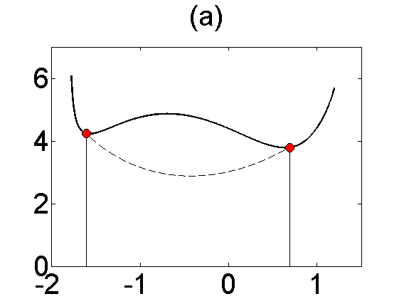
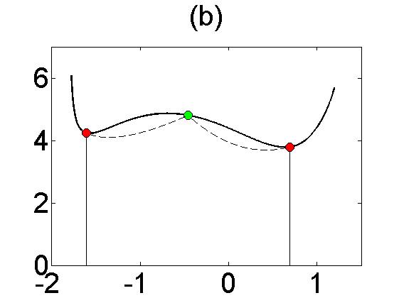
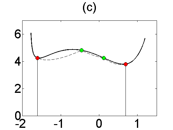
As an illustration, Figure 2 shows four steps of the iterative algorithm. In Figure 2 (a) there are two support points $\mathcal{S}_{j,1}=\{\min{(\mathcal{X}_{j})},\ \max{(\mathcal{X}_{j})}\}$, which yield a single interval $\mathcal{I}_{1,2}=\mathcal{I}_{j}$. In Figures 2 (b)-(c)-(d), we successively add a point $s^{*}$ chosen in the interval $\hat{\mathcal{I}}_{v^{*},v^{*}+1}$ that contains the latest bound. In this example, the point $s^{*}$ is chosen deterministically as the mean of the extremes of the interval $\mathcal{I}_{v^{*},v^{*}+1}$.

Assume that the joint potential is quadratic, i.e., $V^{(n)}_{2}(y_{1}-g_{1,j}(x),\ldots,y_{n}-g_{n,j}(x))=\sum_{i=1}^{n}(y_{i}-g_{i,j}(x))^{2}$ for each $j=1,\ldots,q$, and construct the set of linearities $r_{i,j}(x)=a_{i,j}x+b_{i,j}$, for $i=1,\ldots,n$ and $j=1,\ldots,q$. The modified system potential in $\mathcal{B}_{j}$ becomes

and it turns out straightforward to compute $\gamma_{2,j}=\min\limits_{x\in\mathcal{B}_{j}}V(x;\textbf{y},\textbf{r}_{j})$. Indeed, if we denote $\textbf{a}_{j}=[a_{1,j},\ldots,a_{n,j}]^{\top}$ and $\textbf{w}_{j}=[y_{1}-b_{1,j},\ldots,y_{n}-b_{n,j}]^{\top}$, then we can readily obtain

and $\gamma_{2,j}=V(\tilde{x}_{j};\textbf{y},\textbf{r}_{j})$. It is apparent that $\gamma_{2}=\min\limits_{j}\gamma_{2,j}\leq V(x;\textbf{y},\textbf{g})$. Furthermore, $\tilde{x}_{j}$ is an approximation of the ML estimator $\hat{x}_{j}$ restricted to $\mathcal{B}_{j}$.

If the joint potential is not quadratic, in general it can still be difficult to minimize the modified function $V(x;\textbf{y},\textbf{r})$, despite the replacement of the nonlinearities $g_{i,j}(x)$ with the linear functions $r_{i,j}(x)$. In this section, we propose a method to transform the bound for a quadratic potential, $\gamma_{2}$, into a bound for some other, non-quadratic, potential function.

Consider an arbitrary joint potential $V^{(n)}$ and assume the availability of an invertible increasing function $R$ such that $R\circ V^{(n)}\geq V^{(n)}_{2}$, where $\circ$ denotes the composition of functions. Then, for the system potential we can write

and, as consequence, $V(x;\textbf{y},\textbf{g})\geq R^{-1}\left(\gamma_{2}\right)=\gamma$, hence $\gamma$ is a lower bound for the non-quadratic system potential $V(x;\textbf{y},\textbf{g})$ constructed from $V^{(n)}$.

For instance, consider the family of joint potentials $V^{(n)}_{p}$. Using the monotonicity of $\mathcal{L}^{p}$ norms, it is possible to prove [16] that

Let $R_{1}(v)=v^{2/p}$. Since this function is, indeed, strictly increasing, we can transform the inequality (20) into

which yields

hence the transformation $\gamma_{2}^{p/2}$ of the quadratic bound $\gamma_{2}$ is a lower bound for $V_{p}^{(n)}$ with $0<p\leq 2$. Similarly, if we let $R_{2}(v)=\left(n^{\left(\frac{p-2}{2p}\right)}v^{1/p}\right)^{2}$, the inequality (21) yields

hence the transformation $R_{2}^{-1}(\gamma_{2})=n^{-(p-2)/2}\gamma_{2}^{p/2}$ is a lower bound for $V_{p}^{(n)}$ when $2\leq p<+\infty$.

It is possible to devise a systematic procedure to find a suitable function $R$ given an arbitrary joint potential $V^{(n)}({\mbox{\boldmath$\vartheta$}})$, where ${\mbox{\boldmath$\vartheta$}}\triangleq[\vartheta_{1},\ldots,\vartheta_{n}]^{T}$. Let us define the manifold $\Gamma_{v}\triangleq\left\{{\mbox{\boldmath$\vartheta$}}\in\mathbb{R}^{n}:\ \ V^{(n)}({\mbox{\boldmath$\vartheta$}})=v\right\}$. We can construct $R$ by assigning $R(v)$ with the maximum of the quadratic potential $\sum_{i}^{n}\vartheta_{i}^{2}$ when ${\mbox{\boldmath$\vartheta$}}\in\Gamma_{v}$, i.e., we define

Note that (25) is a constrained optimization problem that can be solved using, e.g., Lagrangian multipliers.

From the definition in (25) we obtain that, $\forall\textbf{{\mbox{\boldmath$\vartheta$}}}\in\Gamma_{v}$, $R(v)\geq\sum_{i=1}^{n}\vartheta_{i}^{2}$. In particular, since $V^{(n)}({\mbox{\boldmath$\vartheta$}})=v$ from the definition of $\Gamma_{v}$, we obtain the desired relationship,

We additionally need to check whether $R$ is a strictly increasing function of $v$. The two functions in the earlier examples of this Section, $R_{1}$ and $R_{2}$, can be readily found using this method.

Assume that $\mathcal{A}=\left\{\mathcal{B}_{j}\right\}_{j=1}^{q}$ and that we have already found $r_{i,j}(x)=a_{i,j}x+b_{i,j}$, $i=1,\ldots,n$ and $j=1,\ldots,q$, using the technique in Section IV-A. If a marginal potential $\bar{V}_{i}(\vartheta_{i})$ is convex, the function $\bar{V}_{i}(y_{i}-r_{i,j}(x))$ is also convex in $\mathcal{B}_{j}$. Indeed, for all $x\in\mathcal{B}_{j}$

where we have used that $\frac{d^{2}r_{i,j}}{dx^{2}}=0$ (since $r_{i,j}$ is linear).

As a consequence, if all marginal potentials $\bar{V}_{i}(\vartheta_{i})$ are convex, then the modified system potential, $V(x;\textbf{y},\textbf{r}_{j})=c_{n}+\sum_{i=1}^{n}\bar{V}_{i}(y_{i}-r_{i,j}(x))$, is also convex in $\mathcal{B}_{j}$. This is easily shown using (27), to obtain

Therefore, we can use the tangents to $V(x;\textbf{y},\textbf{r}_{j})$ at the limit points of $\mathcal{I}_{j}$ (i.e, $\min(\mathcal{X}_{j})$ and $\max(\mathcal{X}_{j})$) to find a lower bound for the system potential $V(x;\textbf{y},\textbf{g}_{j})$. Figure 3 (left) depicts a system potential $V(x;\textbf{y},\textbf{g}_{j})$ (solid line), the corresponding modified potential $V(x;\textbf{y},\textbf{r}_{j})$ (dotted line) and the two tangent lines at $\min(\mathcal{X}_{j})$ and $\max(\mathcal{X}_{j})$. It is apparent that the intersection of the two tangents yields a lower bound in $\mathcal{B}_{j}$. Specifically, if we let $W(x)$ be the piecewise-linear function composed of the two tangents, then the inequality $V(x;\textbf{y},\textbf{g}_{j})\geq V(x;\textbf{y},\textbf{r}_{j})\geq W(x)$ is satisfied for all $x\in\mathcal{I}_{j}$.

References

- (1) A. M. Ali, K. Yao, T. C. Collier, E. Taylor, D. Blumstein, and L. Girod. An empirical study of collaborative acoustic source localization. Proc. Information Processing in Sensor Networks (IPSN07), Boston, April 2007.
- (2) M. H. DeGroot and M. J. Schervish. Probability and Statistics, 3rd ed. Addison-Wesley, New York, 2002.
- (3) P. M. Djurić, J. H. Kotecha, J. Zhang, Y. Huang, T. Ghirmai, M. F. Bugallo, and J. Míguez. Particle filtering. IEEE Signal Processing Magazine, 20(5):19–38, September 2003.
- (4) A. Doucet, N. de Freitas, and N. Gordon, editors. Sequential Monte Carlo Methods in Practice. Springer, New York (USA), 2001.
- (5) M. Evans and T. Swartz. Random variate generation using concavity properties of transformed densities. Journal of Computational and Graphical Statistics, 7(4):514–528, 1998.
- (6) W. J. Fitzgerald. Markov chain Monte Carlo methods with applications to signal processing. Signal Processing, 81(1):3–18, January 2001.
- (7) W. R. Gilks. Derivative-free Adaptive Rejection Sampling for Gibbs Sampling. Bayesian Statistics, (4):641–649, 1992.
- (8) W. R. Gilks and P. Wild. Adaptive Rejection Sampling for Gibbs Sampling. Applied Statistics, 41(2):337–348, 1992.
- (9) W. Hoermann. A rejection technique for sampling from t-concave distributions. ACM Transactions on Mathematical Software, 21(2):182–193, 1995.
- (10) H. R. Künsch. Recursive Monte Carlo filters: Algorithms and theoretical bounds. The Annals of Statistics, 33(5):1983–2021, 2005.
- (11) J. R. Larocque and P. Reilly. Reversible jump mcmc for joint detection and estimation of sources in colored noise. IEEE Transactions on Signal Processing, 50(2), February 1998.
- (12) J. S. Liu. Monte Carlo Strategies in Scientific Computing. Springer, 2004.
- (13) C. P. Robert and G. Casella. Monte Carlo Statistical Methods. Springer, 2004.
- (14) N. G. Best W. R. Gilks and K. K. C. Tan. Adaptive Rejection Metropolis Sampling within Gibbs Sampling. Applied Statistics, 44(4):455–472, 1995.
- (15) N. G. O. Robert W. R. Gilks and E. I. George. Adaptive Direction Sampling. The Statistician, 43(1):179–189, 1994.
- (16) D. Williams. Probability with martingales. Cambridge University Press, Cambridge, (UK), 1991.