跳到论文正文
W Papers独立论文阅读器 arXiv:0904.1180 论文正文 计算阅读时间 · 0%
引用这篇论文根据当前论文元数据生成,正式投稿前建议核对。


License: arXiv.org perpetual non-exclusive license
arXiv:0904.1180v1 [math.PR] 07 Apr 2009

Optimal Hölder exponent for the SLE pathThanks: Johansson is supported by grant KAW 2005.0098 from the Knut and Alice Wallenberg Foundation.Thanks: Lawler is supported by National Science Foundation grant DMS-0734151.

Fredrik Johansson Address: Fredrik Johansson
Department of Mathematics
The Royal Institute of Technology
S – 100 44 Stockholm
SWEDEN
Email address: frejo@math.kth.se
and Gregory F. Lawler Address: Gregory F. Lawler
Department of Mathematics and Department of Statistics
University of Chicago
5734 S. University Avenue
Chicago, IL 60637, USA
Email address: lawler@math.uchicago.edu
Abstract.

We prove an upper bound on the optimal Hölder exponent for the chordal SLE\operatorname{SLE} path parameterized by capacity and thereby establish the optimal exponent as conjectured by J. Lind. We also give a new proof of the lower bound. Our proofs are based on the sharp estimates of moments of the derivative of the inverse map. In particular, we improve an estimate of the second author.

1. Introduction

The Schramm-Loewner evolution, or SLE⁡(κ)\operatorname{SLE}(\kappa), is a one-parameter family of random fractal curves that was introduced by O. Schramm in [Sch00] as a candidate for the scaling limit of the loop-erased random walk. Since then, SLE\operatorname{SLE} has been shown to describe the scaling limits of a number of discrete models from statistical physics and to provide tools for their rigorous understanding. The properties of SLE\operatorname{SLE} curves have been studied by a number of authors. For instance, S. Rohde and Schramm proved in [RS05] the existence and continuity of the path and gave an upper bound on the Hausdorff dimension. V. Beffara [Bef08] proved a lower bound on Hausdorff dimension and thus showed that the dimension is almost surely the minimum of 1+κ/81+\kappa/8 and 22. J. Lind [Lin08] improved the estimates by Rohde and Schramm and proved that the SLE⁡(κ)\operatorname{SLE}(\kappa) path is almost surely Hölder continuous. She conjectured that the Hölder exponent she obtained is the optimal one, that is, that the exponent is the largest possible. In this paper we prove this conjecture. More precisely, we prove the following theorem. Let κ≥0\kappa\geq 0 and set

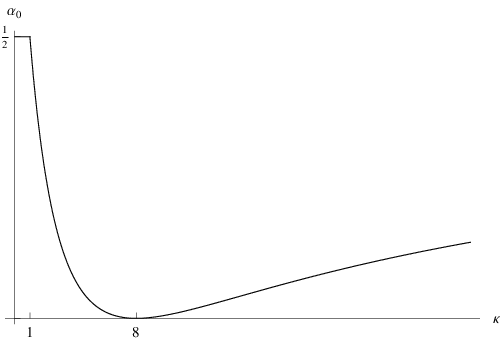
α∗=α∗​(κ)=1−κ24+2​κ−8​8+κ,α0=min⁡{12,α∗}.\alpha_{*}=\alpha_{*}(\kappa)=1-\frac{\kappa}{24+2\kappa-8\sqrt{8+\kappa}},\quad\alpha_{0}=\min\left\{\frac{1}{2},\,\alpha_{*}\right\}.
Theorem 1.1.

Let γ⁡(t)\gamma(t) be the chordal SLE⁡(κ)\operatorname{SLE}(\kappa) path parameterized by half-plane capacity. With probability one the following holds.

  • •

    γ⁡(t),t∈[0,1],\gamma(t),\,t\in[0,1], is Hölder continuous of order α\alpha for α<α0\alpha<\alpha_{0} and is not Hölder continuous of order α\alpha for α>α0.\alpha>\alpha_{0}.

  • •

    For every 0<ϵ<10<\epsilon<1, γ⁡(t),t∈[ϵ,1],\gamma(t),\,t\in[\epsilon,1], is Hölder continuous of order α\alpha for α<α∗\alpha<\alpha_{*} and is not Hölder continuous of order α\alpha for α>α∗.\alpha>\alpha_{*}.

Refer to caption
Figure 1. Optimal Hölder exponent as a function of κ\kappa.

As mentioned, the lower bound on the optimal exponent was proved in [Lin08]. The upper bound is new and we also give a new proof of the lower bound. The phase transition of α0​(κ)\alpha_{0}(\kappa) at κ=1\kappa=1 is due to the geometry of the path at the base; roughly, in the capacity parameterization the path is Hölder-1/21/2 at t=0t=0 for all κ≥0\kappa\geq 0.

The main tool needed is sharp estimates for the moments of the derivative close to the preimage of the tip of the growing curve. We will use the work in [Law09] and also [JL09], but we will have to extend one of these results in this paper. We will use these results as a “black box”, more or less, in the main part of the paper and then give a derivation in the final section, building on the argument in [Law09]. To be more specific, we need to control the growth of the derivative as the preimage of the tip is approached radially. To get the lower bound on the exponent estimates on the derivative from above are needed, and to get the upper bound on the optimal exponent, one has to control second moments and time correlations.

Our paper is organized as follows. In Section 2 we give definitions and discuss some well-known results. In Section 3 we prove a number of results about Loewner chains that are not particular to SLE\operatorname{SLE}, but rather to Loewner chains driven by functions which are weakly Hölder-1/2, see (13) for a definition. Notably, we give estimates on the modulus of continuity of the curve in terms of the radial growth of the derivative. In the Section 4 we state the basic moment estimates and use these together with the results from Section 3 to prove Theorem 1.1. Finally, Section 5 proves the estimates on the derivative. Here we review without proof the main results from [Law09] that we need, and then establish the new estimates.

2. Preliminaries

Let Ut,t≥0U_{t},\,t\geq 0 be a continuous real-valued function. We shall consider chordal Loewner chains (gt)(g_{t}), that is, solutions to the chordal Loewner equation

∂tgt=agt−Ut,t>0,g0​(z)=z,\partial_{t}g_{t}=\frac{a}{g_{t}-U_{t}},\quad t>0,\quad g_{0}(z)=z, (1)

for a>0a>0 fixed. We define the associated continuously growing hull

Kt={z∈ℍ:τ⁡(z)≤t},K_{t}=\{z\in\mathbb{H}:\tau(z)\leq t\},

where τ⁡(z)\tau(z) is the blow-up time of (1). For each t>0t>0 the function z↦gt​(z)z\mapsto g_{t}(z) maps Ht:=ℍ∖KtH_{t}:=\mathbb{H}\setminus K_{t} conformally onto ℍ\mathbb{H} and the inverse mapping ft:=gt−1f_{t}:=g_{t}^{-1} satisfies the partial differential equation

∂tft=−ft′​az−Ut,f0​(z)=z.\partial_{t}f_{t}=-f^{\prime}_{t}\frac{a}{z-U_{t}},\quad f_{0}(z)=z. (2)

Throughout the paper we will use the notation

f^t​(z):=ft​(Ut+z),\hat{f}_{t}(z):=f_{t}(U_{t}+z),

for z∈ℍz\in\mathbb{H}.

The time-reversed Loewner equation

∂tFt=−aFt−UT−t,t∈(0,T],F0​(z)=z\partial_{t}F_{t}=-\frac{a}{F_{t}-U_{T-t}},\quad t\in(0,T],\quad F_{0}(z)=z (3)

is often useful to avoid dealing directly with (2): it is easy to see that if FF is a solution (3) and ff a solution to (2) then

FT​(z)=fT​(z).F_{T}(z)=f_{T}(z).

If there is a curve γ⁡(t)\gamma(t) such that HtH_{t} is the unbounded connected component of ℍ∖γ⁡[0,t]\mathbb{H}\setminus\gamma[0,t] we say that the Loewner chain (gt)(g_{t}) is generated by a curve. This property is known [RS05, Theorem 4.1] to be equivalent to the existence of the radial limit

limy→0f^t​(i​y)=:γ⁡(t)\lim_{y\to 0}\hat{f}_{t}(iy)=:\gamma(t) (4)

for each t>0t>0 together with continuity of t↦γ⁡(t)t\mapsto\gamma(t). Loewner chains corresponding to driving functions with strictly higher regularity than Hölder-1/2 are always generated by a simple curve; in fact Hölder-1/2 continuity with a sufficiently small norm is sufficient to guarantee a simple curve. Conversely, there are examples of Loewner chains corresponding to Hölder-1/2 functions (with large norm) that are not generated by a curve, see [MR05] for these results.

In particular we will be interested in Schramm-Loewner evolution, SLE⁡(κ)\operatorname{SLE}(\kappa), defined as the Loewner chain corresponding to a=2a=2 and Ut=κ​BtU_{t}=\sqrt{\kappa}B_{t}, where BB is standard Brownian motion and κ≥0\kappa\geq 0. SLE\operatorname{SLE} is known to be generated by a curve. We note that the SLE⁡(κ)\operatorname{SLE}(\kappa) path is simple if and only if 0≤κ≤40\leq\kappa\leq 4 and space filling for κ≥8\kappa\geq 8, see [RS05] for proofs of these facts. It may be noted that there is presently no known direct proof of that SLE⁡(8)\operatorname{SLE}(8) is generated by a curve, see [LSW04] for an indrect proof.

Definition 2.1.

A (positive) subpower function is a continuous, non-decreasing function φ:[0,∞)→(0,∞)\varphi:[0,\infty)\to(0,\infty) that satisfies

limx→∞x−ν​φ​(x)=0\lim_{x\to\infty}x^{-\nu}\varphi(x)=0

for all ν>0\nu>0.

3. Deterministic results

In this section we prove a number of results about Loewner chains and associated curves that are not special to SLE\operatorname{SLE}. In particular we consider Loewner chains corresponding to driving functions which are weakly Hölder-1/2, see (13).

For convenience we state the following well-known result, see [Pom92] for a proof.

Lemma 3.1 (The Koebe distortion and one-quarter theorems).

Suppose f:D→ℂf:D\to\mathbb{C} is a conformal map and set d=dist⁡(z,∂D)d=\operatorname{dist}(z,\partial D) for z∈Dz\in D. Then

1−r(1+r)3​|f′​(z)|≤|f′​(w)|≤1+r(1−r)3​|f′​(z)|,|z−w|≤r​d,\frac{1-r}{(1+r)^{3}}|f^{\prime}(z)|\leq|f^{\prime}(w)|\leq\frac{1+r}{(1-r)^{3}}|f^{\prime}(z)|,\quad|z-w|\leq rd, (5)

and

B⁡(f⁡(z),d​|f′​(z)|/4)⊂f⁡(D),B(f(z),d|f^{\prime}(z)|/4)\subset f(D), (6)

where B⁡(w,ρ)B(w,\rho) denotes the open disk of radius ρ\rho around ww.

Lemma 3.2.

Let SS be the rectangle S={x+iy:−1<x<1,0<y<1}S=\{x+iy:-1<x<1,0<y<1\}. There exist c,α<∞c,\alpha<\infty such that if ff is a conformal map defined on 2​S2S, z,w∈Sz,w\in S and Im⁡z,Im⁡w≥1/r\operatorname{Im}\,z,\,\operatorname{Im}\,w\geq 1/r, then

|f′​(z)|≤c​rα​|f′​(w)|.|f^{\prime}(z)|\leq cr^{\alpha}|f^{\prime}(w)|. (7)
Proof.

One way to prove this is to take a conformal transformation of 2​S2S onto the unit disk with f⁡(z)=0f(z)=0 and using the distortion theorem. A more direct approach is as follows. We may assume that Im⁡z=1/r\operatorname{Im}\,z=1/r. Take a Whitney decomposition of SS, that is, a partition of SS into dyadic rectangles {Sj,k}\{S_{j,k}\} where

Sj,k={x+iy:j2−k≤x≤(j+1)2−k, 2−(k+1)≤y≤2−k},S_{j,k}=\{x+iy:j2^{-k}\leq x\leq(j+1)2^{-k},\,2^{-(k+1)}\leq y\leq 2^{-k}\},

for j=0,…,2k−1,j=0,\ldots,2^{k}-1, and k∈ℕk\in\mathbb{N}. Let u,vu,v be in the same rectangle. Then by iterating (5) it follows that there exists a constant c1c_{1} (uniform for all rectangles; 12512^{5} would work for instance) such that

c1−1≤|f′​(u)|/|f′​(v)|≤c1.c_{1}^{-1}\leq|f^{\prime}(u)|/|f^{\prime}(v)|\leq c_{1}. (8)

Suppose that z∈Sj,kz\in S_{j,k}. Then k≤log⁡r≤k+1k\leq\log r\leq k+1. It follows that there exists a path in SS (the hyperbolic geodesic, for instance) that connects zz to ww and intersects at most 2​⌈log⁡r⌉+22\lceil\log r\rceil+2 rectangles. Hence, there is a constant c2c_{2} such that by iterating (8) along the path at most c2​(log⁡r+1)c_{2}(\log r+1) times

|f′​(z)|\displaystyle|f^{\prime}(z)| ≤c1c2​(log⁡r+1)​|f′​(w)|\displaystyle\leq c_{1}^{c_{2}(\log r+1)}|f^{\prime}(w)|
=c​rα​|f′​(w)|,\displaystyle=cr^{\alpha}|f^{\prime}(w)|,

for α=c2​log⁡c1\alpha=c_{2}\log c_{1} and c=c1c2c=c_{1}^{c_{2}}. ∎

A proof of the next lemma may be found in [Law05]. For a set KK, we let diam⁡(K)\operatorname{diam}(K) denotes the diameter of KK and 0​p​t​(K):=sup{Im⁡z:z∈K}0pt(K):=\sup\{\operatorname{Im}\,z:z\in K\}.

Lemma 3.3.

Suppose KtK_{t} is the hull obtained by solving (1) with UtU_{t} as driving function. Let R⁡(t)=t+sup0≤s≤t{|Us−U0|}R(t)=\sqrt{t}+\sup_{0\leq s\leq t}\{|U_{s}-U_{0}|\}. Then there exists a constant c<∞c<\infty such that

c−1​R​(t)≤diam⁡(Kt)≤c​R​(t).c^{-1}R(t)\leq\operatorname{diam}(K_{t})\leq cR(t). (9)
Lemma 3.4.

Let KK be a hull. There exists a constant c<∞c<\infty such that

hcap⁡(K)≤c​diam⁡(K)​ 0​p​t​(K).\operatorname{hcap}(K)\leq c\,\operatorname{diam}(K)\,0pt(K). (10)
Proof.

Let d=diam⁡(K)d=\operatorname{diam}(K) and h=0​p​t​(K)h=0pt(K). We shall only consider the case when h<dh<d (the other case is easily verified by considering the map z↦z+d2/zz\mapsto z+d^{2}/z). By scaling, translation invariance, and monotonicity of hcap\operatorname{hcap} we may assume that d=1d=1 and that KK is contained in the rectangle R={z:|Rez|≤1/2, 0≤Imz≤h}R=\{z:|\operatorname{Re}\,z|\leq 1/2,\,0\leq\operatorname{Im}\,z\leq h\}, so that hcap⁡(K)≤hcap⁡(R)\operatorname{hcap}(K)\leq\operatorname{hcap}(R). It is known that

hcap⁡(R)=limy→∞y​𝔼i​y​(Im⁡B⁡(T)),\operatorname{hcap}(R)=\lim_{y\to\infty}y\,\mathbb{E}^{iy}(\operatorname{Im}\,\,B(T)),

where BB denotes a complex Brownian motion and TT denotes the hitting time of ∂(ℍ∖R)\partial(\mathbb{H}\setminus R), see [Law05]. Hence

hcap⁡(R)≤limy→∞y​ω​(i​y,∂R,ℍ∖R)⋅h,\operatorname{hcap}(R)\leq\lim_{y\to\infty}y\,\omega(iy,\partial R,\mathbb{H}\setminus R)\cdot h,

where ω\omega denotes harmonic measure. Note that RR can be covered by O⁡(h−1)O(h^{-1}) discs of radius 2​h2h centered on the real line. The harmonic measure from i​yiy of any such disc is bounded from above by the harmonic measure of the disc centered at the origin. Since

ω⁡(i​y,∂(2​h​𝔻),ℍ∖(2​h​𝔻))\displaystyle\omega\left(iy,\partial(2h\mathbb{D}),\mathbb{H}\setminus(2h\mathbb{D})\right) =(4/π)​arctan⁡(2​h/y)\displaystyle=(4/\pi)\arctan\left(2h/y\right)
≤c​h/y\displaystyle\leq ch/y

for large yy, the lemma follows from the maximum priciple. ∎

Lemma 3.5.

Suppose ftf_{t} satisfies (2) and z=x+i​y∈ℍz=x+iy\in\mathbb{H}, then for s≥0s\geq 0

e−5as/y2|ft′(z)|≤|ft+s′(z)|≤e5​a​s/y2|ft′(z)|.e^{-5as/y^{2}}\,|f_{t}^{\prime}(z)|\leq|f_{t+s}^{\prime}(z)|\leq e^{5as/y^{2}}\,|f_{t}^{\prime}(z)|. (11)

In particular, if s≤y2s\leq y^{2},

e−5​a​|ft′​(z)|≤|ft+s′​(z)|≤e5​a​|ft′​(z)|.e^{-5a}\,|f_{t}^{\prime}(z)|\leq|f_{t+s}^{\prime}(z)|\leq e^{5a}\,|f_{t}^{\prime}(z)|.

Also, if 0≤s≤y20\leq s\leq y^{2},

|ft+s​(z)−ft​(z)|≤y5​[e5​a−1]​|ft′​(z)|.|f_{t+s}(z)-f_{t}(z)|\leq\frac{y}{5}\,[e^{5a}-1]\,|f_{t}^{\prime}(z)|. (12)
Proof.

Without loss of generality assume that a=1a=1. Differentiating (2) yields

∂tft′​(z)=−ft′′​(z)​1z−Vt+ft′​(z)​1(z−Vt)2.\partial_{t}f_{t}^{\prime}(z)=-f_{t}^{\prime\prime}(z)\,\frac{1}{z-V_{t}}+f_{t}^{\prime}(z)\,\frac{1}{(z-V_{t})^{2}}.

Note that |z−Vt|≥y|z-V_{t}|\geq y. Applying Bieberbach’s theorem (the n=2n=2 case of the Bieberbach conjecture) to the disk of radius yy about zz, we can see that

|ft′′​(z)|≤4​y−1​|ft′​(z)|.|f_{t}^{\prime\prime}(z)|\leq 4\,y^{-1}\,|f_{t}^{\prime}(z)|.

and hence

|∂tft′​(z)|≤5​y−2​|ft′​(z)|,|\partial_{t}f_{t}^{\prime}(z)|\leq 5\,y^{-2}\,|f_{t}^{\prime}(z)|,

which implies (11). Returning to (2), we see that

|∂tft​(z)|≤|ft′​(z)|​aIm⁡(z).|\partial_{t}f_{t}(z)|\leq|f_{t}^{\prime}(z)|\,\frac{a}{\operatorname{Im}\,(z)}.

Using (11), we see that

|ft+s​(z)−ft​(z)|\displaystyle|f_{t+s}(z)-f_{t}(z)| ≤\displaystyle\leq ∫0s|∂sft+s​(z)|​𝑑s\displaystyle\int_{0}^{s}|\partial_{s}f_{t+s}(z)|\,ds
≤\displaystyle\leq a​|ft′​(z)|y​∫0se5​a​s/y2​𝑑s=y5​(e5​a−1)​|ft′​(z)|.\displaystyle\frac{a|f_{t}^{\prime}(z)|}{y}\int_{0}^{s}e^{5as/y^{2}}\,ds=\frac{y}{5}\,(e^{5a}-1)\,|f_{t}^{\prime}(z)|.

∎

We shall consider Loewner chains corresponding to functions that are Hölder continuous of order α\alpha for any α<1/2\alpha<1/2. We say that UU is weakly Hölder-1/2 if there exists a subpower function φ\varphi such that r1/2​φ​(1/r)r^{1/2}\varphi(1/r) is a modulus of continuity for UU, that is,

sup|s|≤r|Ut+s−Ut|≤r1/2​φ​(1/r).\sup_{|s|\leq r}|U_{t+s}-U_{t}|\leq r^{1/2}\varphi(1/r). (13)

By P. Lévy’s theorem the sample paths of Brownian motion are almost surely weakly Hölder-1/2 with subpower function c​log⁡(r)c\sqrt{\log(r)}, c>2c>\sqrt{2}, see [RY99, Theorem I.2.7]. Therefore all results for Loewner chains corresponding to functions that satisfy (13) hold for SLE⁡(κ)\operatorname{SLE}(\kappa) with probability one.

Lemma 3.6.

There exist constants c,α<∞c,\alpha<\infty such that the following holds. Let (gt)(g_{t}) be a Loewner chain corresponding to the continuous function UtU_{t}. Let s∈[0,y2]s\in[0,y^{2}] for y>0y>0. Then

|ft+s′​(Ut+s+i​y)|≤c​Mα​|ft+s′​(Ut+i​y)|,|f^{\prime}_{t+s}(U_{t+s}+iy)|\leq cM^{\alpha}|f^{\prime}_{t+s}(U_{t}+iy)|, (14)

where M=max⁡{|Ut+s−Ut|/y,1}M=\max\{|U_{t+s}-U_{t}|/y,1\}. In particular, if UtU_{t} satisfies (13), then there exists a subpower fuction φ\varphi such that for all tt and all s∈[0,y2]s\in[0,y^{2}],

|ft+s′​(Ut+s+i​y)|≤φ⁡(1/y)​|ft+s′​(Ut+i​y)|.|f^{\prime}_{t+s}(U_{t+s}+iy)|\leq\varphi(1/y)|f^{\prime}_{t+s}(U_{t}+iy)|.
Proof.

We first rescale by |Ut+s−Ut||U_{t+s}-U_{t}|, and then apply Lemma 3.2 with r=max⁡{|Ut+s−Ut|/y,1}r=\max\{|U_{t+s}-U_{t}|/y,1\} to get the conclusion. ∎

The last two lemmas immediately imply the following result, which we record as a lemma. This essentially says that for weakly Hölder-1/2 Loewner chains, it is enough to consider the derivative at dyadic times.

Lemma 3.7.

Let (gt)(g_{t}) be the Loewner chain corresponding to UtU_{t} satisfying (13). Suppose that there exist constants cc and β\beta such that for all n≥1n\geq 1

|f^tk′​(i​2−n)|≤c​2n​β,|\hat{f}^{\prime}_{t_{k}}(i2^{-n})|\leq c2^{n\beta}, (15)

where tk=k2−2​n,k=0,1,…,22​nt_{k}=k2^{-2n},\,k=0,1,\ldots,2^{2n}. Then for every β1>β\beta_{1}>\beta, there exists a constant c1<∞c_{1}<\infty such that

|f^t′​(i​2−n)|≤c1​2n​β1,|\hat{f}^{\prime}_{t}(i2^{-n})|\leq c_{1}2^{n\beta_{1}},

for t∈[0,1]t\in[0,1].

Let (gt)(g_{t}) be the Loewner chain corresponding to a function UtU_{t} satisfying (13) that is generated by a curve γ⁡(t)\gamma(t). We want to estimate the modulus of continuity of γ\gamma. The following quantity will be useful

v⁡(t,y):=∫0y|ft′​(Ut+i​r)|​𝑑r,y>0.v(t,y):=\int_{0}^{y}|f^{\prime}_{t}(U_{t}+ir)|\,dr,\quad y>0. (16)

The geometrical interpretation is of course the length (if it exists) of the image of the segment [Ut,Ut+i​y][U_{t},U_{t}+iy] under ftf_{t}. For a given tt, the limit

γ⁡(t)=limy→0+ft​(Ut+i​y)\gamma(t)=\lim_{y\to 0+}f_{t}(U_{t}+iy) (17)

exists if v⁡(t,y)v(t,y) is finite for some y>0y>0. By integration we have

|γ⁡(t)−ft​(Ut+i​y)|≤v⁡(t,y).|\gamma(t)-f_{t}(U_{t}+iy)|\leq v(t,y).

Using the Koebe one-quarter theorem, we can see that

v⁡(t,y)≥y​|f^t′​(i​y)|/4.v(t,y)\geq\,y\,|\hat{f}_{t}^{\prime}(iy)|/4. (18)

The next result shows that Loewner chains corresponding to weakly Hölder-1/2 functions are generated by a curve if v⁡(t,y)v(t,y) decays polynomially in yy. We also get an estimate of the modulus of continuity of the curve.

Proposition 3.8.

Let (gt)(g_{t}) be the Loewner chain corresponding to UtU_{t} satisfying (13). Then there exists a subpower function φ\varphi such that if 0≤t≤t+s≤10\leq t\leq t+s\leq 1 and s∈[0,y2]s\in[0,y^{2}]

|γ⁡(t+s)−γ⁡(t)|≤φ⁡(1/y)​[v⁡(t+s,y)+v⁡(t,y)].|\gamma(t+s)-\gamma(t)|\leq\varphi(1/y)\left[v(t+s,y)+v(t,y)\right]. (19)
Remark.

We have not assumed existence of the curve in this proposition. If v⁡(t+s,y),v⁡(t,y)<∞v(t+s,y),v(t,y)<\infty, then we know that radial limit (4) exists, so we can write γ⁡(t),γ⁡(t+s)\gamma(t),\gamma(t+s). If one of the radial limits does not exist we can define γ\gamma any way that we want since the right hand side of (19) is infinite.

Proof.

We start by writing

|γ⁡(t+s)−γ⁡(t)|≤|γ⁡(t+s)−ft+s​(Ut+s+i​y)|+|γ⁡(t)−ft​(Ut+i​y)||\gamma(t+s)-\gamma(t)|\leq|\gamma(t+s)-f_{t+s}(U_{t+s}+iy)|+|\gamma(t)-f_{t}(U_{t}+iy)|
+|ft+s​(Ut+s+i​y)−ft+s​(Ut+i​y)|+|ft+s​(Ut+i​y)−ft​(Ut+i​y)|.+|f_{t+s}(U_{t+s}+iy)-f_{t+s}(U_{t}+iy)|+|f_{t+s}(U_{t}+iy)-f_{t}(U_{t}+iy)|.

We have to estimate the last two terms. Note that

|ft+s​(Ut+s+i​y)−ft+s​(Ut+i​y)|≤|Ut+s−Ut|​max⁡|ft+s′​(w)|,|f_{t+s}(U_{t+s}+iy)-f_{t+s}(U_{t}+iy)|\leq|U_{t+s}-U_{t}|\,\max|f_{t+s}^{\prime}(w)|,

where the maximum is over all ww on the line segment connecting Ut+s+i​yU_{t+s}+iy and Ut+i​yU_{t}+iy. By Lemma 3.6 using assumption (13) and then by (18), we see that

|ft+s​(Ut+s+i​y)−ft+s​(Ut+i​y)|\displaystyle|f_{t+s}(U_{t+s}+iy)-f_{t+s}(U_{t}+iy)| ≤c​φ​(1/y)​y​|ft+s′​(Ut+s+i​y)|\displaystyle\leq c\,\varphi(1/y)\,y\,|f_{t+s}^{\prime}(U_{t+s}+iy)|
≤c​φ​(1/y)​v​(t+s,y).\displaystyle\leq c\,\varphi(1/y)\,v(t+s,y).

By (12) and (18)

|ft+s​(Ut+i​y)−ft​(Ut+i​y)|\displaystyle|f_{t+s}(U_{t}+iy)-f_{t}(U_{t}+iy)| ≤y5​[e5​a−1]​|ft′​(Ut+i​y)|\displaystyle\leq\frac{y}{5}\,[e^{5a}-1]\,|f_{t}^{\prime}(U_{t}+iy)|
≤c⁡[e5​a−1]​v​(t,y).\displaystyle\leq c\,[e^{5a}-1]\,v(t,y).

∎

Proposition 3.9.

Let (gt)(g_{t}) be the Loewner chain corresponding to UtU_{t} satisfying (13). Suppose that (gt)(g_{t}) is generated by a curve γ⁡(t)\gamma(t). Then for each tt, there exist t1,t2∈[t,t+y2]t_{1},t_{2}\in[t,t+y^{2}], and constants c,δ>0c,\delta>0 such that

|γ⁡(t1)−γ⁡(t2)|≥c​|f^t′​(i​y)|​y​φ​(1/y)−δ.|\gamma(t_{1})-\gamma(t_{2})|\geq c\,|\hat{f}^{\prime}_{t}\left(iy\right)|y\varphi\left(1/y\right)^{-\delta}.
Proof.

Let β:=gt​(γ⁡[t,t+y2])\beta:=g_{t}(\gamma[t,t+y^{2}]). Then β\beta is the curve obtained by solving (1) with Ut+r,r∈[0,y2],U_{t+r},\,r\in[0,y^{2}], as driving function. Hence hcap⁡(β)=a​y2\operatorname{hcap}(\beta)=ay^{2}, and by Lemma 3.3 together with the assumption (13) on UU,

ρd:=diam⁡(β)≤y​φ​(1/y).\rho_{d}:=\operatorname{diam}(\beta)\leq y\,\varphi\left(1/y\right). (20)

Next, we combine (20) with Lemma 3.4 to find

ρh:=0​p​t​(β)≥c​y​φ​(1/y)−1,\rho_{h}:=0pt(\beta)\geq c\,y\,\varphi\left(1/y\right)^{-1}, (21)

for some constant cc. Let z∈βz\in\beta satisfy Im⁡z≥ρh\operatorname{Im}\,z\geq\rho_{h}. Note that |Re⁡z−Ut|≤diam⁡(β)≤ρd|\operatorname{Re}\,z-U_{t}|\leq\operatorname{diam}(\beta)\leq\rho_{d}. By scaling by ρd−1\rho_{d}^{-1} and then using Lemma 3.2 with r=φ​(1/y)2r=\varphi(1/y)^{2} we get

|ft′​(z)|≥c​φ​(1/y)−2​α​|f^t′​(i​y)|,|f_{t}^{\prime}(z)|\geq c\,\varphi(1/y)^{-2\alpha}|\hat{f}^{\prime}_{t}(iy)|, (22)

where α\alpha is the exponent from Lemma 3.2. Let ww be a point on β\beta such that |w−z|=ρh/2|w-z|=\rho_{h}/2. Since z,w∈βz,w\in\beta there are t1,t2∈[t,t+y2]t_{1},t_{2}\in[t,t+y^{2}] such that γ⁡(t1)=ft​(z)\gamma(t_{1})=f_{t}(z) and γ⁡(t2)=ft​(w)\gamma(t_{2})=f_{t}(w). In view of (6) we have

B⁡(ft​(z),|ft′​(z)|​ρh/16)⊂ft​(B⁡(z,ρh/4)),B(f_{t}(z),|f_{t}^{\prime}(z)|\rho_{h}/16)\subset f_{t}(B(z,\rho_{h}/4)), (23)

where B⁡(z,ρ)B(z,\rho) denotes the open ball of radius ρ\rho around zz. Hence, using (23) and (22), we conclude that

|γ⁡(t1)−γ⁡(t2)|\displaystyle|\gamma(t_{1})-\gamma(t_{2})| =|ft​(z)−ft​(w)|\displaystyle=|f_{t}(z)-f_{t}(w)|
≥|ft′​(z)|​ρh/16\displaystyle\geq|f_{t}^{\prime}(z)|\,\rho_{h}/16
≥c​|f^t′​(i​y)|​y​φ​(1/y)−(2​α+1),\displaystyle\geq c\,|\hat{f}^{\prime}_{t}(iy)|\,y\,\varphi(1/y)^{-(2\alpha+1)},

and this completes the proof. ∎

Although we do not use it in this paper, we will give some results about existence of the curve for continuous driving functions that are not necessarily weakly Hölder-1/21/2.

Proposition 3.10.

There exists c<∞c<\infty such that the following is true. Suppose δ>0\delta>0 and (gt)(g_{t}) is a Loewner chain with driving function UtU_{t}. Suppose that 0≤s,y<∞0\leq s,y<\infty and

|Ut+s−Us|≤δ.|U_{t+s}-U_{s}|\leq\delta. (24)

Then

|γ⁡(t+s)−γ⁡(t)|≤c​e5​a​[v⁡(t,δ)+v⁡(t+s,δ)].|\gamma(t+s)-\gamma(t)|\leq c\,e^{5a}\,\left[v(t,\delta)+v(t+s,\delta)\right].
Proof.

We use the triangle inequality on |γ⁡(t+s)−γ⁡(t)||\gamma(t+s)-\gamma(t)| as in the beginning of the proof of Proposition 3.8 with y=δy=\delta. The first two terms are bounded by v⁡(t+s,δ)v(t+s,\delta) and v⁡(t,δ)v(t,\delta), respectively, and the fourth term is bounded in the same way. The distortion theorem, (24), and (18) imply

|ft+s​(Ut+s+i​δ)−ft+s​(Ut+i​δ)|\displaystyle|f_{t+s}(U_{t+s}+i\delta)-f_{t+s}(U_{t}+i\delta)| ≤c​δ​|ft+s′​(Ut+s+i​δ)|\displaystyle\leq c\,\delta\,|f^{\prime}_{t+s}(U_{t+s}+i\delta)|
≤c​v​(t+s,δ),\displaystyle\leq c\,v(t+s,\delta),

and we get the desired estimate. ∎

Corollary 3.11.

Suppose (gt)(g_{t}) is a Loewner chain with continuous driving function UtU_{t}. Suppose that for each 0<t1<t2<∞0<t_{1}<t_{2}<\infty,

limy→0+v⁡(t,y)=0\lim_{y\rightarrow 0+}v(t,y)=0

uniformly for t∈[t1,t2]t\in[t_{1},t_{2}]. Then (gt)(g_{t}) is generated by a curve.

Proof.

Since γ\gamma is a uniform limit of a sequence of continuous functions on [t1,t2][t_{1},t_{2}], γ\gamma is continuous on [t1,t2][t_{1},t_{2}]. One can check directly from the Loewner equation that γ\gamma is right continuous at 00 and hence γ\gamma is continuous. ∎

Remark.

This result also gives an estimate for the modulus of continuity of γ\gamma. However, the assumptions are very strong. If we do not assume that UtU_{t} is weakly Hölder-1/21/2, we do not have Lemma 3.7.

4. Proof of Theorem 1.1

We now turn to the proof of our main result. The proof of Theorem 1.1 is split into two parts: the lower bound (which requires derivative estimates from above) is proven in Subsection 4.1 and the upper bound (wich requires estimates from below and control of correlations) in Subsection 4.2. The SLE\operatorname{SLE} moment estimates (Lemma 4.1 and Lemma 4.4) we need for the proof are only stated in this section. The proofs of the estimates build on those in [Law09] and are discussed in the last section.

To state the lemmas it is convenient to introduce a number of κ\kappa-dependent parameters. Suppose

−∞<r<rc:=12+4κ.-\infty<r<r_{c}:=\frac{1}{2}+\frac{4}{\kappa}.

The significance of rcr_{c} is discussed in Section 5. Let

λ=λ⁡(r)=r⁡(1+κ4)−κ​r28,\lambda=\lambda(r)=r\,\left(1+\frac{\kappa}{4}\right)-\frac{\kappa r^{2}}{8},
ζ=ζ⁡(r)=r−κ​r28,\zeta=\zeta(r)=r-\frac{\kappa r^{2}}{8},

and

β=β⁡(r)=−1+κ4+κ−κ​r.\beta=\beta(r)=-1+\frac{\kappa}{4+\kappa-\kappa r}.

Note that β\beta and λ\lambda strictly increase with rr for −∞<r<rc-\infty<r<r_{c} and hence, we could alternatively consider either of them as the free parameter. Let r+r_{+} be the larger root to λ​β+ζ=2\lambda\beta+\zeta=2 and let β+,λ+\beta_{+},\,\lambda_{+} and ζ+\zeta_{+} be the corresponding values of β,λ\beta,\lambda and ζ\zeta respectively. Note that if κ≠8\kappa\neq 8, then r+<rcr_{+}<r_{c} and

−1=β⁡(−∞)<β+=−1+κ12+κ−4​8+κ<β⁡(rc)=1.-1=\beta(-\infty)<\beta_{+}=-1+\frac{\kappa}{12+\kappa-4\sqrt{8+\kappa}}<\beta(r_{c})=1.

Also,

α∗=1−β+2.\alpha_{*}=\frac{1-\beta_{+}}{2}.

4.1. Lower bound

The following is the main moment estimate for the lower bound. This was proved in [Law09] for a certain range of rr including r=1,κ<8r=1,\kappa<8 which was most important for that paper. We give a different proof here that is valid for all r<rcr<r_{c}.

Lemma 4.1.

Suppose r<rcr<r_{c}. Then there exists c<∞c<\infty such that for all t≥1t\geq 1

𝔼⁡[|f^t2′​(i)|λ]≤c​t−ζ.\mathbb{E}\left[|\hat{f}_{t^{2}}^{\prime}(i)|^{\lambda}\right]\leq c\,t^{-\zeta}. (25)
Proof.

See Section 5. ∎

In the proof of this result one also finds that the expectation in (25), roughly speaking, is carried on an event on which |f^t2′​(i)|≈tβ|\hat{f}_{t^{2}}^{\prime}(i)|\approx t^{\beta} and this has probability of order t−(ζ+λ​β).t^{-(\zeta+\lambda\beta)}. From this lemma we can derive the following uniform estimate from which the lower bound will follow. Recall that f^0′​(i​y)=1\hat{f}^{\prime}_{0}(iy)=1 for all y>0y>0, so we have to restrict our attention to positive β\beta.

Proposition 4.2.

Suppose β>max⁡{0,β+}\beta>\max\{0,\beta_{+}\}. With probability one there exists y0>0y_{0}>0, such that for all t∈[0,1]t\in[0,1] and all y<y0y<y_{0},

|f^t′​(i​y)|≤y−β.|\hat{f}_{t}^{\prime}(iy)|\leq y^{-\beta}.
Proof.

For β>max⁡{0,β+}\beta>\max\{0,\beta_{+}\} we have λ>0,ζ>0\lambda>0,\zeta>0 and β​λ+ζ>2\beta\lambda+\zeta>2. By choosing β\beta smaller if necessary, but still larger than max⁡{0,β+}\max\{0,\beta_{+}\}, we can guarantee that ζ<2\zeta<2. We write

f^j,n=f^(j−1)​2−2​n,j=1,…,22​n.\hat{f}_{j,n}=\hat{f}_{(j-1)2^{-2n}},\quad j=1,\ldots,2^{2n}.

By Lemma 3.7 and the distortion theorem it suffices to prove that for all β>max⁡{0,β+}\beta>\max\{0,\beta_{+}\}, with probability one there exists N<∞N<\infty such that for n≥Nn\geq N,

|f^j,n′(i2−n)|≤2β​n,j=1,2,…,22​n.|\hat{f}_{j,n}^{\prime}(i2^{-n})|\leq 2^{\beta n},\quad j=1,2,\ldots,2^{2n}. (26)

Note that scale invariance implies

ℙ{|f^j,n′(i2−n)|≥2β​n}=ℙ{|f^j−1′(i)|≥2β​n}.\mathbb{P}\left\{|\hat{f}_{j,n}^{\prime}(i2^{-n})|\geq 2^{\beta n}\right\}=\mathbb{P}\left\{|\hat{f}_{j-1}^{\prime}(i)|\geq 2^{\beta n}\ \right\}.

By Lemma 4.1 and Chebyshev’s inequality,

ℙ{|f^j−1′(i)|≥2β​n}≤2−λ​β​n𝔼[|f^j−1′(i)|λ]\mathbb{P}\left\{|\hat{f}_{j-1}^{\prime}(i)|\geq 2^{\beta n}\ \right\}\leq 2^{-\lambda\beta n}\,\mathbb{E}\left[|\hat{f}_{j-1}^{\prime}(i)|^{\lambda}\right]\hskip 72.26999pt
≤c​j−ζ2​ 2−λ​β​n=c​(j22​n)−ζ2​2−n⁡(λ​β+ζ).\hskip 72.26999pt\leq c\,j^{-\frac{\zeta}{2}}\,2^{-\lambda\beta n}=c\,\left(\frac{j}{2^{2n}}\right)^{-\frac{\zeta}{2}}2^{-n(\lambda\beta+\zeta)}.

Since λ​β+ζ>2\lambda\beta+\zeta>2 and ζ<2\zeta<2, we can sum over jj to get

∑j=122​nℙ{|f^j−1′(i)|≥2β​n}≤c 2−n⁡(λ​β+ζ−2),\sum_{j=1}^{2^{2n}}\mathbb{P}\left\{|\hat{f}_{j-1}^{\prime}(i)|\geq 2^{\beta n}\ \right\}\leq c\,2^{-n(\lambda\beta+\zeta-2)}, (27)

and hence

∑n=1∞∑j=122​nℙ{|f^j−1′(i)|≥2β​n}<∞.\sum_{n=1}^{\infty}\sum_{j=1}^{2^{2n}}\mathbb{P}\left\{|\hat{f}_{j-1}^{\prime}(i)|\geq 2^{\beta n}\ \right\}<\infty.

The Borel-Cantelli lemma now implies (26). ∎

Proposition 4.3.

Suppose β+<β<0\beta_{+}<\beta<0. With probability one, for every ϵ>0\epsilon>0, there exists yϵ>0y_{\epsilon}>0 such that for all t∈[ϵ,1]t\in[\epsilon,1] and all y<yϵy<y_{\epsilon},

|ft′​(i​y)|≤y−β.|f_{t}^{\prime}(iy)|\leq y^{-\beta}.
Proof.

For β+<β<0\beta_{+}<\beta<0, we have λ​β+ζ>2\lambda\beta+\zeta>2 and λ>0\lambda>0. The proof is identical to the previous proposition except that we do not have ζ>0\zeta>0. We replace (27) with

∑ϵ​22​n≤j≤22​nℙ{|f^j−1′(i)|≥2β​n}≤cϵ 2−n⁡(λ​β+ζ−2).\sum_{\epsilon 2^{2n}\leq j\leq 2^{2n}}\mathbb{P}\left\{|\hat{f}_{j-1}^{\prime}(i)|\geq 2^{\beta n}\ \right\}\leq c_{\epsilon}\,2^{-n(\lambda\beta+\zeta-2)}.

∎

We can now easily prove the lower bound in Theorem 1.1. Recall that α∗=min⁡{1/2,(1−β+)/2}\alpha_{*}=\min\{1/2,(1-\beta_{+})/2\}.

Proof of lower bound for Theorem 1.1.

Let 1≥β>β~>max⁡{0,β+}1\geq\beta>\tilde{\beta}>\max\{0,\beta_{+}\}; recall that β+=1\beta_{+}=1 if and only if κ=8\kappa=8. Almost surely, by Proposition 4.2, we have for all t∈[0,1]t\in[0,1]

v⁡(t,y)=∫0y|f^t′​(i​r)|​𝑑r≤y1−β~v(t,y)=\int_{0}^{y}|\hat{f}_{t}^{\prime}(ir)|\,dr\leq y^{1-\tilde{\beta}} (28)

if yy is small enough. The last inequality together with Proposition 3.8 show that the SLE⁡(κ)\operatorname{SLE}(\kappa) Loewner chain is generated by a curve when κ≠8\kappa\neq 8 and imply the following modulus of continuity

|γ⁡(t+s)−γ⁡(t)|≤c​s(1−β)/2|\gamma(t+s)-\gamma(t)|\leq cs^{(1-\beta)/2}

for all ss small enough since β~>β\tilde{\beta}>\beta. The lower bound follows.

If β+<β<0\beta_{+}<\beta<0, it suffices to prove the result for each fixed ϵ\epsilon. The argument is the same using Proposition 4.3 ∎

4.2. Upper bound

In this subsection we shall use the notation

f^j,n=f^(j−1)/n2,j=n2/2,…,n2.\hat{f}_{j,n}=\hat{f}_{(j-1)/n^{2}},\quad j=n^{2}/2,\ldots,n^{2}.
Lemma 4.4.

Suppose r<rcr<r_{c}. Then there exist 0<c1,c2<∞0<c_{1},c_{2}<\infty, a subpower function φ{\varphi}, and events

Ej,n,n=1,2,…,j=1,…,n2E_{j,n},\;\;\;n=1,2,\ldots,\;\;j=1,\ldots,n^{2}

such that the following hold. Let E⁡(j,n)=1Ej,nE(j,n)=1_{E_{j,n}} and

F⁡(j,n)=nζ−2​|f^j,n′​(i/n)|λ​E​(j,n).F(j,n)=n^{\zeta-2}\,|\hat{f}_{j,n}^{\prime}(i/n)|^{\lambda}\,E(j,n).
  • •

    If n2/2≤j≤n2n^{2}/2\leq j\leq n^{2}, then on the event Ej,nE_{j,n},

    |f^j,n′​(i/n)|≥φ​(n)−1​nβ.|\hat{f}_{j,n}^{\prime}(i/n)|\geq{\varphi}(n)^{-1}\,n^{\beta}. (29)
  • •

    If n2/2≤j≤nn^{2}/2\leq j\leq n,

    c1​n−2≤𝔼⁡[F⁡(j,n)]≤c2​n−2.c_{1}\,n^{-2}\leq\mathbb{E}\left[F(j,n)\right]\leq c_{2}\,n^{-2}. (30)
  • •

    If n2/2≤j≤k≤n2n^{2}/2\leq j\leq k\leq n^{2},

    𝔼⁡[F⁡(j,n)​F​(k,n)]≤n−4​(n2k−j+1)λ​β+ζ2​φ​(n2k−j+1).\mathbb{E}[F(j,n)\,F(k,n)]\leq n^{-4}\,\left(\frac{n^{2}}{k-j+1}\right)^{\frac{\lambda\beta+\zeta}{2}}\,{\varphi}\left(\frac{n^{2}}{k-j+1}\right). (31)
Proof.

See Section 5.2. ∎

For fixed β\beta, we let An=An,βA_{n}=A_{n,\beta} denote the event that there exists an integer jj with 1≤j≤n21\leq j\leq n^{2},

|f^j,n′​(i/n)|≥φ​(n)−1​nβ,|\hat{f}_{j,n}^{\prime}(i/n)|\geq{\varphi}(n)^{-1}\,n^{\beta}, (32)

where φ{\varphi} is as in (29) We then have the following.

Lemma 4.5.

Suppose λ​β+ζ<2\lambda\beta+\zeta<2. Then there exist c>0c>0 such for all nn sufficiently large,

ℙ⁡(An)≥c.\mathbb{P}(A_{n})\geq c.

In particular,

ℙ​{An​ i.o.}≥c.\mathbb{P}\{A_{n}\mbox{ i.o.}\}\geq c.
Proof.

Let F⁡(j,n)F(j,n) be as in Lemma 4.4, and let

Yn=∑j=n2/2n2F⁡(j,n).Y_{n}=\sum_{j=n^{2}/2}^{n^{2}}F(j,n).

Note that An⊃{Yn>0}A_{n}\supset\{Y_{n}>0\}. The estimates from Lemma 4.4 show that there exist 0<c<c2<∞0<c<c_{2}<\infty such that

𝔼⁡[Yn]≥c,𝔼⁡[Yn2]≤c22.\mathbb{E}[Y_{n}]\geq c,\;\;\;\;\mathbb{E}[Y_{n}^{2}]\leq c_{2}^{2}.

(This uses β​λ+ζ<2\beta\lambda+\zeta<2.) Therefore, a standard second moment argument gives

ℙ(An)≥ℙ{Yn>0}≥𝔼​[Yn]2𝔼⁡[Yn2]≥c2c22.\mathbb{P}(A_{n})\geq\mathbb{P}\{Y_{n}>0\}\geq\frac{\mathbb{E}[Y_{n}]^{2}}{\mathbb{E}[Y_{n}^{2}]}\geq\frac{c^{2}}{c_{2}^{2}}.

∎

We can now prove the upper bound for Theorem 1.1 and thereby complete the proof. Notice that Proposition 3.9 immediately implies that γ⁡[0,t]\gamma[0,t] cannot be Hölder continuous of order >1/2>1/2, since f^0′​(z)=1\hat{f}^{\prime}_{0}(z)=1.

Proof of upper bound for Theorem 1.1.

Let β<β~<β+\beta<\tilde{\beta}<\beta_{+}. Proposition 3.9 implies that on the event An=An,β~A_{n}=A_{n,\tilde{\beta}} there exist times t1,t2∈[0,1]t_{1},t_{2}\in[0,1] such that

|γ⁡(t1)−γ⁡(t2)|≥c​nβ−1=c​(n−2)(1−β)/2,|t1−t2|≤n−2.|\gamma(t_{1})-\gamma(t_{2})|\geq cn^{\beta-1}=c(n^{-2})^{(1-\beta)/2},\quad|t_{1}-t_{2}|\leq n^{-2}.

Consequently on the event {Ani.o}\{A_{n}\,\,\rm{i.o}\}, the curve γ⁡(t),t∈[0,1]\gamma(t),\,t\in[0,1], is not Hölder continuous of order (1−β)/2(1-\beta)/2. To show that this happens almost surely, let 𝒜r\mathcal{A}_{r} be the event that γ⁡(t),t∈[0,r]\gamma(t),\,t\in[0,r], is not Hölder continuous of order (1−β)/2(1-\beta)/2. By Lemma 4.5 we have

ℙ⁡(𝒜1)=:c0>0,\mathbb{P}(\mathcal{A}_{1})=:c_{0}>0,

and by scale invariance

ℙ⁡(𝒜r)=c0,r>0.\mathbb{P}(\mathcal{A}_{r})=c_{0},\quad r>0.

Note that 𝒜r⊂𝒜1\mathcal{A}_{r}\subset\mathcal{A}_{1} if r≤1r\leq 1 so that

ℙ⁡(⋂r>0𝒜r)=c0.\mathbb{P}\left(\bigcap_{r>0}\mathcal{A}_{r}\right)=c_{0}.

Since c0>0c_{0}>0, it now follows from the Blumenthal zero-one law (see [RY99, Theorem III.2.15]) that c0=1c_{0}=1 and this completes the proof. ∎

5. Moments of derivatives

In this section we review some results from [Law09] and extend one result. We fix κ\kappa and we let a=2/κa=2/\kappa. We also fix a real number rr such that

r<rc=1+4​a2.r<r_{c}=\frac{1+4a}{2}.

All constants and parameters in this section depend on aa and rr. We let

q=rc−r=2​a+12−r>0.q=r_{c}-r=2a+\frac{1}{2}-r>0.

The positivity of qq is important for the arguments in this section and this is why rr must be less than rcr_{c}.

A useful tool for estimating moments of |f^t′||\hat{f}_{t}^{\prime}| is the reverse Loewner flow (see, e.g., [Law09, Section 10.3]). Suppose UtU_{t} is a standard Brownian motion and ht​(z)h_{t}(z) is the solution to the reverse-time Loewner equation

∂tht​(z)=aUt−ht​(z),h0​(z)=z.\partial_{t}h_{t}(z)=\frac{a}{U_{t}-h_{t}(z)},\;\;\;\;h_{0}(z)=z. (33)

For fixed TT, the distribution of hT​(z)−UTh_{T}(z)-U_{T} is the same as that of f^T​(z)\hat{f}_{T}(z) and hence, hT′​(z)h_{T}^{\prime}(z) has the same distribution as f^T′​(z)\hat{f}_{T}^{\prime}(z). Indeed, suppose gtg_{t} is the solution of the forward-time equation for some continuous VV with V0=0V_{0}=0:

∂tgt​(z)=agt​(z)−Vt,\partial_{t}g_{t}(z)=\frac{a}{g_{t}(z)-V_{t}},

and we let Vt(T)=VT−t−VTV^{(T)}_{t}=V_{T-t}-V_{T}. Then if hh is a solution to (33) with driving function Vt(T)V_{t}^{(T)} we have

gT−1​(z+VT)=hT​(z)+VT=hT​(z)−VT(T).g_{T}^{-1}(z+V_{T})=h_{T}(z)+V_{T}=h_{T}(z)-V_{T}^{(T)}.

It remains to note that Vt(T), 0≤t≤TV_{t}^{(T)},\,0\leq t\leq T, is a standard Brownian motion starting at 00 if VV is. If S<TS<T and h(S),h(T)h^{(S)},h^{(T)} denote the solutions to (33) with driving functions Ut(S)=US−t−USU_{t}^{(S)}=U_{S-t}-U_{S} and Ut(T)=UT−t−UTU_{t}^{(T)}=U_{T-t}-U_{T} then ht(T),0≤t≤T−Sh^{(T)}_{t},0\leq t\leq T-S and ht(S),0≤t≤Sh^{(S)}_{t},0\leq t\leq S are independent. Note that f^S′​(z)​f^T′​(z)\hat{f}_{S}^{\prime}(z)\,\hat{f}_{T}^{\prime}(z) has the same distribution as (hS(S))′​(z)​(hT(T))′​(z)(h_{S}^{(S)})^{\prime}(z)\,(h_{T}^{(T)})^{\prime}(z).

Let Zt=Zt​(i)=Xt+i​Yt=ht​(i)−UtZ_{t}=Z_{t}(i)=X_{t}+iY_{t}=h_{t}(i)-U_{t} and St=sin[argZt]=[1+Xt2/Yt2]−1/2S_{t}=\sin[\arg Z_{t}]=[1+X^{2}_{t}/Y^{2}_{t}]^{-1/2}. To study the behavior of ht′​(i)h_{t}^{\prime}(i), it is useful to do a time-change so that the the logarithm of the imaginary part grows linearly. Let

σ⁡(t)=inf{s:Ys​(z)=ea​t}.\sigma(t)=\inf\{s:Y_{s}(z)=e^{at}\}.

The following lemma can be deduced from the Loewner equation and the analogous time change in a stochastic differential equation.

Lemma 5.1.

[Law09, Section 5] Suppose JtJ_{t} satisifes

dJt=−rctanhJtdt+dWt,J0=0,dJ_{t}=-r_{c}\,\tanh J_{t}\,dt+dW_{t},\;\;\;\;J_{0}=0, (34)

where WtW_{t} is standard Brownian motion. Let

Lt=t−∫0t2​d​scosh2⁡Js,L_{t}=t-\int_{0}^{t}\frac{2\,ds}{\cosh^{2}J_{s}},
σ⁡(t)=∫0te2​a​s​cosh2⁡Js​𝑑s,η⁡(s)=σ−1​(s).\sigma(t)=\int_{0}^{t}e^{2as}\,\cosh^{2}J_{s}\;ds,\;\;\;\;\eta(s)=\sigma^{-1}(s). (35)

Then the joint distribution of

ea​Lη⁡(s),ea​η​(s),cosh⁡Jη⁡(s),     0≤s<∞e^{aL_{\eta(s)}},\;\;\;\;e^{a\eta(s)},\;\;\;\;\cosh J_{\eta(s)},\;\;\;\;\;0\leq s<\infty

is the same as that of

|hs′​(i)|,Ys,Ss−1,    0≤s<∞.|h_{s}^{\prime}(i)|,\;\;\;\;Y_{s},\;\;\;\;S_{s}^{-1},\;\;\;\;0\leq s<\infty.

Let λ,ζ,β\lambda,\zeta,\beta be as in Section 4; we can write

λ=r⁡(1+12​a)−r24​a,ζ=λ−r2​a,\lambda=r\,\left(1+\frac{1}{2a}\right)-\frac{r^{2}}{4a},\;\;\;\;\zeta=\lambda-\frac{r}{2a},
β=1−2​q1+2​q=r−2​a1−2​r+2​a.\beta=\frac{1-2q}{1+2q}=\frac{r-2a}{1-2r+2a}.

We comment here that the β\beta of this paper is the same as μ\mu in [Law09]; the β\beta in that paper is half this value.

Note that (34) can be written as

dJt=−(q+r)tanhJtdt+dWt,J0=0.dJ_{t}=-(q+r)\,\tanh J_{t}\,dt+dW_{t},\;\;\;\;J_{0}=0.

Using Itô’s formula, one can see that

Nt=ea​λ​Lt​ea​ζ​t​[cosh⁡Jt]rN_{t}=e^{a\lambda L_{t}}\,e^{a\zeta t}\,[\cosh J_{t}]^{r}

is a martingale satisfying

d​Nt=r⁡[tanh⁡Jt]​Nt​d​Wt.dN_{t}=r\,[\tanh J_{t}]\,N_{t}\,dW_{t}.

Let ℙ∗\mathbb{P}_{*} denote the probability measure obtained by weighting by the martingale NtN_{t}, that is, if EE is an event measurable with respect to {Ws:0≤s≤t}\{W_{s}:0\leq s\leq t\},

ℙ∗​(E)=N0−1​𝔼​[Nt​ 1E]=𝔼⁡[Nt​ 1E].\mathbb{P}_{*}(E)=N_{0}^{-1}\,\mathbb{E}[N_{t}\,1_{E}]={\mathbb{E}[N_{t}\,1_{E}]}.

The Girsanov theorem (see, e.g., [RY99, Chapter VIII] and [Law09, Appendix A]) implies that

dWt=rtanhJtdt+dBt,dW_{t}=r\,\tanh J_{t}\,dt+dB_{t},
dJt=−qtanhJtdt+dBt,dJ_{t}=-q\,\tanh J_{t}\,dt+dB_{t}, (36)

where BtB_{t} is a standard Brownian motion with respect to the measure ℙ∗\mathbb{P}_{*}. We write 𝔼∗\mathbb{E}_{*} for expectations with respect to ℙ∗\mathbb{P}_{*}.

Lemma 5.2.

[Law09, Lemma 7.1] Suppose JtJ_{t} satisfies (36).

  • •

    JtJ_{t} is a positive recurrent diffusion (with respect to the measure ℙ∗\mathbb{P}_{*}) with invariant density

    v⁡(x)=Γ⁡(q+12)Γ⁡(12)​Γ​(q)​1cosh2​q⁡x.v(x)=\frac{\Gamma(q+\frac{1}{2})}{\Gamma(\frac{1}{2})\Gamma(q)}\,\frac{1}{\cosh^{2q}x}.
  • •
    ∫−∞∞[1−2cosh2⁡x]​v​(x)​𝑑x=1−2​q1+2​q=β.\int_{-\infty}^{\infty}\left[1-\frac{2}{\cosh^{2}x}\right]\,v(x)\,dx=\frac{1-2q}{1+2q}=\beta.
  • •

    Assume J0=0J_{0}=0. There exists c<∞c<\infty such that if k≥0k\geq 0, u≥0u\geq 0,

    ℙ∗{coshJt≥u for some k≤t≤k+1}≤cu−2​q.\mathbb{P}_{*}\{\cosh J_{t}\geq u\mbox{ for some }k\leq t\leq k+1\}\leq c\,u^{-2q}. (37)
Lemma 5.3.

There exists c<∞c<\infty such that the following holds. Suppose JtJ_{t} satisfies (36) with J0=x>0.J_{0}=x>0.

  • •

    If y>xy>x,

    ℙ∗{max0≤s≤1|Js|≥y}≤cexp{−(y−x)22}.\mathbb{P}_{*}\left\{\max_{0\leq s\leq 1}|J_{s}|\geq y\right\}\leq c\,\exp\left\{-\frac{(y-x)^{2}}{2}\right\}. (38)
  • •

    If y<xy<x and 1≤t<(x−y)/q1\leq t<(x-y)/q,

    ℙ∗{min0≤s≤tJs≤y}≤cexp{−(x−q​t−y)22​t}.\mathbb{P}_{*}\left\{\min_{0\leq s\leq t}J_{s}\leq y\right\}\leq c\,\exp\left\{-\frac{(x-qt-y)^{2}}{2t}\right\}. (39)
Proof.

Since the drift of JtJ_{t} points towards the origin, the distribution of |Jt||J_{t}| is stochastically dominated by the absolute value of a Brownian motion. Hence by the reflection principle (see, e.g., [RY99, Proposition III.3.7]) if VV is a standard Brownian motion

ℙ∗{max0≤s≤1|Js|≥y}\displaystyle\mathbb{P}_{*}\left\{\max_{0\leq s\leq 1}|J_{s}|\geq y\right\} ≤ℙ∗{max0≤s≤1|Vs|≥y−x}\displaystyle\leq\mathbb{P}_{*}\left\{\max_{0\leq s\leq 1}|V_{s}|\geq y-x\right\}
≤4ℙ∗{V1≥y−x},\displaystyle\leq 4\,\mathbb{P}_{*}\left\{V_{1}\geq y-x\right\},

which gives the first estimate. Also, Jt≥J~tJ_{t}\geq\tilde{J}_{t} where J~t\tilde{J}_{t} satisfies

d​J~t=−q​d​t+d​Bt.d\tilde{J}_{t}=-q\,dt+dB_{t}.

Note that Wt:=J~t+t​q−xW_{t}:=\tilde{J}_{t}+tq-x is a standard Brownian motion starting at the origin. We get for y<xy<x and 1≤t<(x−y)/q1\leq t<(x-y)/q, again using the reflection principle,

ℙ∗{min0≤s≤tJs≤y}\displaystyle\mathbb{P}_{*}\left\{\min_{0\leq s\leq t}J_{s}\leq y\right\} ≤ℙ∗{max0≤s≤tWs≥x−y−qt}\displaystyle\leq\mathbb{P}_{*}\left\{\max_{0\leq s\leq t}W_{s}\geq x-y-qt\right\}
=2ℙ∗{Wt≥x−y−qt},\displaystyle=2\,\mathbb{P}_{*}\left\{W_{t}\geq x-y-qt\right\},

and the second estimate follows. ∎

5.1. Proof of Lemma 4.1

Lemma 4.1 extends a result in [Law09] where the result was proved for a certain range of rr (including r=1,a>1/4r=1,a>1/4 which was most important for that paper). We start by restating it in terms of hh with an added lower bound (and upgrading it to a theorem).

Theorem 5.4.

If r<rcr<r_{c}, there exists 0<c1,c2<∞0<c_{1},c_{2}<\infty such that for all t≥1t\geq 1,

c1​t−ζ≤𝔼⁡[|ht2′​(i)|λ]≤c2​t−ζ.c_{1}\,t^{-\zeta}\leq\mathbb{E}\left[|h_{t^{2}}^{\prime}(i)|^{\lambda}\right]\leq c_{2}\,t^{-\zeta}.

The heuristic argument is fairly straightforward, so let us consider that first. Consider the martingale NtN_{t} which we can write as

Nt=|hσ⁡(t)′​(i)|λ​ea​t​ζ​Sσ⁡(t)−r.N_{t}=|h_{\sigma(t)}^{\prime}(i)|^{\lambda}\,e^{at\zeta}\,S_{\sigma(t)}^{-r}.

We know that 𝔼⁡[Nt]=1\mathbb{E}[N_{t}]=1. If r<rcr<r_{c}, then under ℙ∗\mathbb{P}_{*}, since JJ is positive recurrent, Sσ⁡(s)S_{\sigma(s)} tends to be of order 11 for s<ts<t. Hence we would expect that σ⁡(t)≈e2​a​t\sigma(t)\approx e^{2at} and hence we would expect

𝔼⁡[|he2​a​t′​(i)|λ​ea​t​ζ]≍1.\mathbb{E}\left[|h_{e^{2at}}^{\prime}(i)|^{\lambda}\,e^{at\zeta}\right]\asymp 1.

We will only prove the upper bound in Theorem 5.4 in this subsection; the lower bound follows from the work of the next subsection, which uses the upper bound. The next lemma gives a quantitative bound on the assertion σ⁡(t)≈e2​a​t\sigma(t)\approx e^{2at}. As a slight abuse of notation, in this section, if EE is an event we also write EE for the indicator function of the event.

Lemma 5.5.

There exists c<∞c<\infty such that for all u>0u>0,

ℙ∗{σ(t)≥u2e2​a​t}≤cu−2​q.\mathbb{P}_{*}\{\sigma(t)\geq u^{2}\,e^{2at}\}\leq c\,u^{-2q}. (40)
Proof.

Suppose cosh⁡Js≤u​ea⁡(t−s)​(t−s+1)−1\cosh J_{s}\leq u\,e^{a(t-s)}\,(t-s+1)^{-1} for all 0≤s≤t0\leq s\leq t. Then,

σ⁡(t)=∫0te2​a​s​cosh2⁡Js​𝑑s≤u2​e2​a​t​∫0t(t−s+1)−2​𝑑s<u2​e2​a​t.\sigma(t)=\int_{0}^{t}e^{2as}\,\cosh^{2}J_{s}\,ds\leq u^{2}\,e^{2at}\,\int_{0}^{t}(t-s+1)^{-2}\,ds<u^{2}e^{2at}.

Therefore,

ℙ∗{σ(t)≥u2e2​a​t}≤ℙ∗[⋃k=1∞Kk]≤∑k=1∞ℙ∗(Kk),\mathbb{P}_{*}\{\sigma(t)\geq u^{2}\,e^{2at}\}\leq\mathbb{P}_{*}\left[\bigcup_{k=1}^{\infty}K_{k}\right]\leq\sum_{k=1}^{\infty}\mathbb{P}_{*}(K_{k}),

where Kk=Kk,tK_{k}=K_{k,t} denotes the event

Kk={coshJt−s≥uea⁡(k−1)(k+1)−1 for some k−1≤s<k}.K_{k}=\left\{\cosh J_{t-s}\geq ue^{a(k-1)}\,(k+1)^{-1}\mbox{ for some }k-1\leq s<k\right\}. (41)

By (37),

ℙ∗​(Kk)≤c​u−2​q​e−2​a​q​k​k2​q,\mathbb{P}_{*}(K_{k})\leq c\,u^{-2q}\,e^{-2aqk}\,k^{2q}, (42)

and hence we can sum over kk to get the result. ∎

The next lemma is a useful “smoothing” result that lets us consider the average of 𝔼⁡[|hs′​(i)|λ]\mathbb{E}[|h^{\prime}_{s}(i)|^{\lambda}] over t2≤s≤2​t2t^{2}\leq s\leq 2t^{2} instead of 𝔼[ht2′(i)|λ]\mathbb{E}[h^{\prime}_{t^{2}}(i)|^{\lambda}].

Lemma 5.6.

There exists c<∞c<\infty such that

𝔼⁡[|ht2′​(i)|λ]\displaystyle\mathbb{E}\left[|{h_{t^{2}}}^{\prime}(i)|^{\lambda}\right] ≤ct2​∫0∞e2​a​s​𝔼​[(cosh2⁡Js)​|hσ⁡(s)′​(i)|λ​Is]​𝑑s\displaystyle\leq\frac{c}{t^{2}}\int_{0}^{\infty}e^{2as}\,\mathbb{E}\left[(\cosh^{2}J_{s})\,|h_{\sigma(s)}^{\prime}(i)|^{\lambda}\,I_{s}\right]\,ds
=ct2​∫0∞ea​s​(2−ζ)​𝔼∗​[(cosh⁡Js)2−r​Is]​𝑑s,\displaystyle=\frac{c}{t^{2}}\int_{0}^{\infty}e^{as(2-\zeta)}\,\mathbb{E}_{*}\left[(\cosh J_{s})^{{2-r}}\,I_{s}\right]\,ds,

where Is=Is,tI_{s}=I_{s,t} denotes the event

Is={t2≤σ(s)≤2t2}.I_{s}=\{t^{2}\leq\sigma(s)\leq 2\,t^{2}\}.
Proof.

By scaling and the distortion theorem, if t2≤u≤2​t2t^{2}\leq u\leq 2t^{2},

𝔼⁡[|hu′​(i)|λ]=𝔼⁡[|ht2′​(i​t/u)|λ]≥c​𝔼​[|ht2′​(i)|λ].\mathbb{E}\left[{|h_{u}}^{\prime}(i)|^{\lambda}\right]=\mathbb{E}\left[{|h_{t^{2}}}^{\prime}(it/\sqrt{u})|^{\lambda}\right]\geq c\,\mathbb{E}\left[|{h_{t^{2}}}^{\prime}(i)|^{\lambda}\right].

Therefore,

𝔼⁡[|ht2′​(i)|λ]≤ct2​∫t22​t2𝔼⁡[|hu′​(i)|λ]​𝑑u.\mathbb{E}\left[|{h_{t^{2}}}^{\prime}(i)|^{\lambda}\right]\leq\frac{c}{t^{2}}\int_{t^{2}}^{2t^{2}}\mathbb{E}\left[|{h_{u}}^{\prime}(i)|^{\lambda}\right]\,du.

If we let s=σ−1​(u)s=\sigma^{-1}(u), we can change variables and write

∫t22​t2|hu′​(i)|λ​𝑑u=∫0∞|hσ⁡(s)′​(i)|λ​Is​𝑑u=∫0∞e2​a​s​(cosh2⁡Js)​|hσ⁡(s)′​(i)|λ​Is​𝑑s.\int_{t^{2}}^{2t^{2}}|{h_{u}}^{\prime}(i)|^{\lambda}\,du=\int_{0}^{\infty}|h_{\sigma(s)}^{\prime}(i)|^{\lambda}\,I_{s}\,du=\int_{0}^{\infty}e^{2as}\,(\cosh^{2}J_{s})\,|h_{\sigma(s)}^{\prime}(i)|^{\lambda}\,I_{s}\,ds.

By taking expectations we get the inequality in the lemma, and the equality follows from the definition of 𝔼∗\mathbb{E}_{*}. ∎

Since

σ⁡(t)≥∫0te2​a​s​𝑑s=12​a​[e2​a​t−1],\sigma(t)\geq\int_{0}^{t}e^{2as}\,ds=\frac{1}{2a}\,\left[e^{2at}-1\right],

there is a cc such that Is,ea​tI_{s,e^{at}} is empty if s≥t+cs\geq t+c. Hence the previous proposition implies that there exists a c<∞c<\infty such that

𝔼⁡[|he2​a​t′​(i)|λ]≤\mathbb{E}\left[|{h_{e^{2at}}}^{\prime}(i)|^{\lambda}\right]\leq\hskip 108.405pt
ce−2​a​t∫0t+cea​s​(2−ζ)𝔼∗[(coshJs)2−r;e2​a​t≤σ(s)≤2e2​a​t]ds.c\,e^{-2at}\,\int_{0}^{t+c}e^{as(2-\zeta)}\,\mathbb{E}_{*}\left[(\cosh J_{s})^{{2-r}}\,;\,e^{2at}\leq\sigma(s)\leq 2e^{2at}\right]\,ds. (43)
Lemma 5.7.

There exists c<∞c<\infty such that if u≥1u\geq 1,

𝔼∗[(coshJt)2−r;u2≤e−2​a​tσ(t)≤2u2]≤cu(2−r)+−2​q.\mathbb{E}_{*}[(\cosh J_{t})^{{2-r}};u^{2}\leq e^{-2at}\,\sigma(t)\leq 2u^{2}]\leq c\,u^{(2-r)_{+}-2q}.
Remark.

Roughly speaking, we expect that if σ⁡(t)≍u2​e2​a​t\sigma(t)\asymp u^{2}\,e^{2at}, then cosh⁡Jt≈u\cosh J_{t}\approx u. Hence, we would guess

𝔼∗[(coshJt)2−r;u2≤e−2​a​tσ(t)≤2u2]≈\mathbb{E}_{*}[(\cosh J_{t})^{{2-r}};u^{2}\leq e^{-2at}\,\sigma(t)\leq 2u^{2}]\approx\hskip 72.26999pt
u2−rℙ∗{u2≤e−2​a​tσ(t)≤2u2}≤cu2−r−2​q,\hskip 72.26999ptu^{2-r}\,\mathbb{P}_{*}\{u^{2}\leq e^{-2at}\,\sigma(t)\leq 2u^{2}\}\leq c\,u^{2-r-2q},

where the probability is estimated by (40). This lemma makes the argument rigorous but only gives a weaker result for r>2r>2. Lemma 5.8 below establishes the stronger result for some values of r>2r>2.

Proof.

Let It=It,uI_{t}=I_{t,u} be the the event {u2≤e−2​a​tσ(t)≤2u2}.\{u^{2}\leq e^{-2at}\,\sigma(t)\leq 2u^{2}\}. We claim that ItI_{t} is contained in the event

A=At,u={min(t−1)∨0≤s≤tcosh2Js≤2u2e2​a}A=A_{t,u}=\left\{\min_{(t-1)\vee 0\leq s\leq t}\cosh^{2}J_{s}\leq 2u^{2}e^{2a}\right\}

Indeed, this is obvious for t≤1t\leq 1 since cosh⁡J0=1\cosh J_{0}=1 and if t>1t>1 and cosh2⁡Js>2​e2​a​u2\cosh^{2}J_{s}>2e^{2a}u^{2} for t−1≤s≤tt-1\leq s\leq t, then

σ⁡(t)≥∫t−1te2​a​s​cosh2⁡Js​𝑑s>2​u2​e2​a​t.\sigma(t)\geq\int_{t-1}^{t}e^{2as}\,\cosh^{2}J_{s}\,ds>2u^{2}\,e^{2at}.

Let

Vk=Vk,t,u=It∩{ue(k−1)≤coshJt<uek}.V_{k}=V_{k,t,u}=I_{t}\cap\left\{u\,e^{(k-1)}\leq\cosh J_{t}<u\,e^{k}\ \right\}.

Then,

𝔼∗​[(cosh⁡Jt)2−r​It]=∑k=−∞∞𝔼∗​[(cosh⁡Jt)2−r​Vk].\mathbb{E}_{*}[(\cosh J_{t})^{{2-r}}\,I_{t}]=\sum_{k=-\infty}^{\infty}\mathbb{E}_{*}[(\cosh J_{t})^{{2-r}}\,V_{k}].

Note that

𝔼∗​[(cosh⁡Jt)2−r​Vk]≍u2−r​ek⁡(2−r)​ℙ∗​(Vk).\mathbb{E}_{*}[(\cosh J_{t})^{{2-r}}\,V_{k}]\asymp u^{2-r}\,e^{k(2-r)}\,\mathbb{P}_{*}(V_{k}). (44)

We will first show that

∑k=1∞𝔼∗​[(cosh⁡Jt)2−r​Vk]≤c​u2−r−2​q.\sum_{k=1}^{\infty}\mathbb{E}_{*}[(\cosh J_{t})^{{2-r}}\,V_{k}]\leq c\,u^{2-r-2q}. (45)

Let k0k_{0} be an integer such that ek−1>2​e2​ae^{k-1}>2e^{2a} for k≥k0k\geq k_{0}. Then,

∑k=1k0𝔼∗​[(cosh⁡Js)2−r​Vk]\displaystyle\sum_{k=1}^{k_{0}}\mathbb{E}_{*}[(\cosh J_{s})^{{2-r}}\,V_{k}] ≍u2−r​∑k=1k0ℙ∗​(Vk)\displaystyle\asymp u^{2-r}\sum_{k=1}^{k_{0}}\mathbb{P}_{*}(V_{k})
≤u2−rℙ∗{cosh2Jt≥u2}≤cu2−r−2​q.\displaystyle\leq u^{2-r}\,\mathbb{P}_{*}\{\cosh^{2}J_{t}\geq u^{2}\}\leq cu^{2-r-2q}.

The last inequality uses (37).

If k>k0k>k_{0}, let

ηt=inf{s≥(t−1)∨0:cosh2⁡Js=2​e2​a​u2}.\eta_{t}=\inf\left\{s\geq(t-1)\vee 0:\cosh^{2}J_{s}=2e^{2a}u^{2}\right\}.

Since Vk⊂AV_{k}\subset A and cosh2⁡Jt>2​e2​a​s​u2\cosh^{2}J_{t}>2e^{2as}u^{2} on VkV_{k}, we know that on the event VkV_{k}, t−1≤ηt<tt-1\leq\eta_{t}<t. Hence we can estimate

ℙ∗(Vk)≤ℙ∗{ηt<t}ℙ∗{cosh2Jt≥u2ek−1∣ηt<t}.\mathbb{P}_{*}(V_{k})\leq\mathbb{P}_{*}\{\eta_{t}<t\}\,\mathbb{P}_{*}\left\{\cosh^{2}J_{t}\geq u^{2}\,e^{k-1}\;\mid\;\eta_{t}<t\right\}.

By (37),

ℙ∗{ηt<t}≤ℙ∗{cosh2Js≥2e2​au2 for some t−1≤s≤t}≤cu−2​q.\mathbb{P}_{*}\{\eta_{t}<t\}\leq\mathbb{P}_{*}\left\{\cosh^{2}J_{s}\geq 2e^{2a}u^{2}\mbox{ for some }t-1\leq s\leq t\right\}\leq c\,u^{-2q}.

Using (38), we can see that there exist c,αc,\alpha such that

ℙ∗​{cosh2⁡Jt≥u2​ek−1∣ηt<t}≤c​e−α​k2.\mathbb{P}_{*}\left\{\cosh^{2}J_{t}\geq u^{2}\,e^{k-1}\;\mid\;\eta_{t}<t\right\}\leq c\,e^{-\alpha k^{2}}.

Hence, plugging into (44), we have

𝔼∗​[(cosh⁡Jt)2−r​Vk]≤c​u2−r−2​q​ek⁡(2−r)​e−α​k2.\mathbb{E}_{*}[(\cosh J_{t})^{{2-r}}\,V_{k}]\leq c\,u^{2-r-2q}\,e^{k(2-r)}\,e^{-\alpha k^{2}}.

Therefore,

u2​q+r−2​∑k=1∞𝔼∗​[(cosh⁡Jt)2−r​Vk]≤c​∑k=0∞ek⁡(2−r)​e−α​k2<∞.u^{2q+r-2}\,\sum_{k=1}^{\infty}\mathbb{E}_{*}[(\cosh J_{t})^{{2-r}}\,V_{k}]\leq c\sum_{k=0}^{\infty}e^{k(2-r)}\,e^{-\alpha k^{2}<\infty}.

This proves (45).

Let V~=⋃k=0∞V−k.\tilde{V}=\bigcup_{k=0}^{\infty}V_{-k}. On the event V~\tilde{V},

1≤cosh⁡Jt≤u.1\leq\cosh J_{t}\leq u.

Hence (cosh⁡Jt)2−r≤u(2−r)+(\cosh J_{t})^{2-r}\leq u^{(2-r)_{+}} and, using (40),

𝔼∗​[(cosh⁡Jt)2−r​V~]≤u(2−r)+​ℙ∗​(V~)≤u(2−r)+​ℙ∗​(It)≤c​u(2−r)+​u−2​q.\mathbb{E}_{*}[(\cosh J_{t})^{{2-r}}\,\tilde{V}]\leq u^{(2-r)_{+}}\,\mathbb{P}_{*}(\tilde{V})\leq u^{(2-r)_{+}}\,\mathbb{P}_{*}(I_{t})\leq c\,u^{(2-r)_{+}}\,u^{-2q}.

∎

Lemma 5.8.

If r>a+1r>a+1, there exists c<∞c<\infty such that for all uu,

𝔼∗[(coshJt)2−r;u2≤e−2​a​tσ(t)≤2u2]≤cu2−r−2​q.\mathbb{E}_{*}[(\cosh J_{t})^{{2-r}};u^{2}\leq e^{-2at}\,\sigma(t)\leq 2u^{2}]\leq c\,u^{2-r-2q}.
Proof.

We use the notation from the proof of Lemma 5.7 and let Vj=V−jV^{j}=V_{-j}. We note that (45) holds for all values of rr. Hence, we only need to show

∑j=0∞𝔼∗​[(cosh⁡Jt)2−r​Vj]≤c​u2−r−2​q.\sum_{j=0}^{\infty}\mathbb{E}_{*}[(\cosh J_{t})^{{2-r}}\,V^{j}]\leq c\,u^{2-r-2q}.

Let KkK_{k} be as in (41). Then

∑j=0∞𝔼∗​[(cosh⁡Jt)2−r​Vj]≤∑k=1∞∑j=0∞𝔼∗​[(cosh⁡Jt)2−r​Vj​Kk].\sum_{j=0}^{\infty}\mathbb{E}_{*}[(\cosh J_{t})^{{2-r}}\,V^{j}]\leq\sum_{k=1}^{\infty}\sum_{j=0}^{\infty}\mathbb{E}_{*}[(\cosh J_{t})^{2-r}\,V^{j}\,K_{k}].

Note that

u2​q+r−2​𝔼∗​[(cosh⁡Jt)2−r​Vj​Kk]\displaystyle u^{2q+r-2}\,\mathbb{E}_{*}[(\cosh J_{t})^{2-r}\,V^{j}\,K_{k}] ≍u2​q​ej⁡(r−2)​ℙ∗​(Vj∩Kk)\displaystyle\asymp u^{2q}e^{j(r-2)}\,\mathbb{P}_{*}(V^{j}\cap K_{k})
=u2​q​ℙ∗​(Kk)​ej⁡(r−2)​ℙ∗​(Vj∣Kk).\displaystyle=u^{2q}\,\mathbb{P}_{*}(K_{k})\,e^{j(r-2)}\,\mathbb{P}_{*}(V^{j}\mid K_{k}).

By (42), we know that u2​q​ℙ∗​(Kk)≤c​e−2​a​q​k​k2​qu^{2q}\,\mathbb{P}_{*}(K_{k})\leq c\,e^{-2aqk}\,k^{2q}. Hence, it suffices to prove that

∑k=1∞e−2​a​q​k​k2​q​∑j=0∞ej⁡(r−2)​ℙ∗​(Vj∣Kk)<∞.\sum_{k=1}^{\infty}e^{-2aqk}\,k^{2q}\sum_{j=0}^{\infty}e^{j(r-2)}\,\mathbb{P}_{*}(V^{j}\mid K_{k})<\infty. (46)

Note that for 1+a<r<rc1+a<r<r_{c}, we have a>qa>q and

−2​a​q+(r−2)22+(2−r)​(a−q)<0,-2aq+\frac{(r-2)^{2}}{2}+(2-r)\,(a-q)<0,

Choose a^\hat{a} satisfying q<a^<aq<\hat{a}<a and

−2​a^​q+(r−2)22+(2−r)​(a^−q)<0,-2\hat{a}q+\frac{(r-2)^{2}}{2}+(2-r)\,(\hat{a}-q)<0, (47)

We will show

∑k=1∞e−2​a^​q​k​∑j=0∞ej⁡(r−2)​ℙ∗​(Vj∣Kk)<∞.\sum_{k=1}^{\infty}e^{-2\hat{a}qk}\sum_{j=0}^{\infty}e^{j(r-2)}\,\mathbb{P}_{*}(V^{j}\mid K_{k})<\infty.

On the event KkK_{k}, let ss be the largest number less than or equal to kk such that

cosh⁡Jt−s≥u​ea⁡(k−1)​(k+1)−1.\cosh J_{t-s}\geq ue^{a(k-1)}\,(k+1)^{-1}.

By the definition of Kk,K_{k}, we know that k−1≤s≤kk-1\leq s\leq k. Also, we can find c1c_{1} such that

Jt−s≥log⁡u+a⁡(k−1)−log⁡(k+1)≥log⁡u+a^​k−c1+log⁡2.J_{t-s}\geq\log u+a(k-1)-\log(k+1)\geq\log u+\hat{a}k-c_{1}+\log 2.

On the event VjV^{j}, cosh⁡Jt≤e−j​u\cosh J_{t}\leq e^{-j}u which implies

Jt≤log⁡u−j+log⁡2.J_{t}\leq\log u-j+\log 2.

We estimate ℙ∗​(Vj∣Kk)\mathbb{P}_{*}(V^{j}\mid K_{k}) from above by

supk−1≤s≤kℙ∗​{Jt≤log⁡u−j+log⁡2∣Jt−s=log⁡u+a^​k−c1+log⁡2}.\sup_{k-1\leq s\leq k}\mathbb{P}_{*}\left\{J_{t}\leq\log u-j+\log 2\mid J_{t-s}=\log u+\hat{a}k-c_{1}+\log 2\right\}.

As in (39), this probability is bounded above by the corresponding probability if JtJ_{t} is a Brownian motion with drift −q-q. In particular, (39) shows that there exists MM and c2c_{2} such that for j>Mj>M,

ℙ∗​(Vj∣Kk)≤c​exp⁡{−12​k​[(a^−q)​k+j−c1]2}.\mathbb{P}_{*}(V^{j}\mid K_{k})\leq c\,\exp\left\{-\frac{1}{2k}\,[(\hat{a}-q)k+j-c_{1}]^{2}\right\}. (48)

Note that

∑k=1∞e−2​a^​q​k​∑j=0Mej⁡(r−2)​ℙ∗​(Vj∣Kk)≤∑k=1∞e−2​a^​q​k​∑j=0Mej⁡(r−2)<∞.\sum_{k=1}^{\infty}e^{-2\hat{a}qk}\sum_{j=0}^{M}e^{j(r-2)}\,\mathbb{P}_{*}(V^{j}\mid K_{k})\leq\sum_{k=1}^{\infty}e^{-2\hat{a}qk}\sum_{j=0}^{M}e^{j(r-2)}<\infty.

Also, (48) gives

∑j=M+1∞ej⁡(r−2)​ℙ∗​(Vj∣Kk)≤c​∑j=M+1∞exp⁡{j⁡(r−2)−12​k​[j+b]2}.\sum_{j=M+1}^{\infty}e^{j(r-2)}\,\mathbb{P}_{*}(V^{j}\mid K_{k})\leq c\sum_{j=M+1}^{\infty}\exp\left\{j(r-2)-\frac{1}{2k}\,[j+b]^{2}\right\}.

where

b=(a^−q)​k−c2.b=(\hat{a}-q)k-c_{2}.

We bound the right hand side from above by a constant times

∫−∞∞ex⁡(r−2)​e−(x+b)22​k​𝑑x\displaystyle\int_{-\infty}^{\infty}e^{x(r-2)}e^{-\frac{(x+b)^{2}}{2k}}\,dx =eb⁡(2−r)​∫−∞∞ey⁡(r−2)​e−y22​k​𝑑y\displaystyle=e^{b(2-r)}\int_{-\infty}^{\infty}e^{y(r-2)}e^{-\frac{y^{2}}{2k}}\,dy
≤c​k​exp⁡{b⁡(2−r)+k​(r−2)22}\displaystyle\leq c\,\sqrt{k}\,\exp\left\{b(2-r)+\frac{k(r-2)^{2}}{2}\right\}
≤c​k​exp⁡{(2−r)​(a^−q)​k+k​(r−2)22}\displaystyle\leq c\,\sqrt{k}\,\exp\left\{(2-r)(\hat{a}-q)k+\frac{k(r-2)^{2}}{2}\right\}

Hence

e−2​a^​q​k​∑j=M+1∞ej⁡(r−2)​ℙ∗​(Vj∣Kk)≤Cϵ​k​ek​ξe^{-2\hat{a}qk}\,\sum_{j={M+1}}^{\infty}e^{j(r-2)}\mathbb{P}_{*}(V^{j}\mid K_{k})\leq C_{\epsilon}\,\sqrt{k}\,e^{k\xi}

where

ξ=−2​a^​q+(2−r)​(a^−q)+(r−2)22.\xi=-2\hat{a}q+(2-r)(\hat{a}-q)+\frac{(r-2)^{2}}{2}.

Recalling from (47) that ξ<0\xi<0, we conclude

∑k=1∞e−2​a^​q​k​∑j=M+1∞ej⁡(r−2)​ℙ∗​(Vj∣Kk)<∞.\sum_{k=1}^{\infty}e^{-2\hat{a}qk}\,\sum_{j={M+1}}^{\infty}e^{j(r-2)}\mathbb{P}_{*}(V^{j}\mid K_{k})<\infty.

∎

Lemma 5.9.

Suppose r<rcr<r_{c}. Then there exists θ<2−ζ\theta<2-\zeta and c<∞c<\infty such that for all uu

𝔼∗[(coshJt)2−r;u2≤e−2​a​tσ(t)≤2u2]≤cuθ.\mathbb{E}_{*}[(\cosh J_{t})^{{2-r}};u^{2}\leq e^{-2at}\,\sigma(t)\leq 2u^{2}]\leq c\,u^{\theta}. (49)
Proof.

We set

θ={2−r−2​q, if ​r≤2​ or ​r≥a+12−2​qotherwise.\theta=\left\{\begin{array}[]{ll}2-r-2q,&\mbox{ if }r\leq 2\mbox{ or }r\geq a+\frac{1}{2}\\ -2q&\mbox{otherwise}.\end{array}\right.

The estimate (49) follows from the previous two lemmas so we only need to verify that θ<2−ζ\theta<2-\zeta. It is easy to see that 1−r−2​q<2−ζ1-r-2q<2-\zeta for all rr. Also, one can check that −2​q<1−4​a+r-2q<1-4a+r provided that a<3/5a<3/5 or a≥3/5a\geq 3/5 and

r<2​a​[3−5−(3/a)].r<2a\,\left[3-\sqrt{5-(3/a)}\right]. (50)

If a≤4a\leq 4, then one can show that (50) holds for all r<rcr<r_{c}. Hence we only need to consider a≥4a\geq 4 and r<rcr<r_{c} that do not satisfy (50). Such an rr satisfies

r≥2​a​[3−5−(3/a)]≥2​a​[3−17/4]≥9​a/5.r\geq 2a\,\left[3-\sqrt{5-(3/a)}\right]\geq 2a\,[3-\sqrt{17/4}]\geq 9a/5.

In particular, r>a+1r>a+1. ∎

Proof of Theorem 5.4.

Let θ\theta be as in the previous lemma. Then by (49),

𝔼∗[(coshJs)2−r;e2​a​t≤σ(s)≤2e2​a​t]≤ce(t−s)​a​θ.\mathbb{E}_{*}\left[(\cosh J_{s})^{{2-r}}\,;\,e^{2at}\leq\sigma(s)\leq 2e^{2at}\right]\leq ce^{(t-s)a\theta}.

Therefore, by (43),

𝔼⁡[|he2​a​t′​(i)|λ]\displaystyle\mathbb{E}\left[|h_{e^{2at}}^{\prime}(i)|^{\lambda}\right] ≤c​e−2​a​t​∫0t+ce2​a​s​e−a​s​ζ​e(t−s)​a​θ​𝑑s\displaystyle\leq c\,e^{-2at}\,\int_{0}^{t+c}\,e^{2as}\,e^{-as\zeta}\,e^{(t-s)a\theta}\,ds
≤c​e−a​ζ​t​∫0t+cea⁡(t−s)​[−2+ζ+θ]​𝑑s.\displaystyle\leq c\,e^{-a\zeta t}\,\int_{0}^{t+c}e^{a(t-s)[-2+\zeta+\theta]}\,ds.
≤c​e−a​ζ​t​∫−c∞ea​y​[−2+ζ+θ]​𝑑y≤c​e−a​ζ​t.\displaystyle\leq c\,e^{-a\zeta t}\,\int_{-c}^{\infty}e^{ay[-2+\zeta+\theta]}\,dy\leq c\,e^{-a\zeta t}.

The last inequality uses θ<2−ζ.\theta<2-\zeta.

∎

5.2. Proof of Lemma 4.4

We essentially follow the proof in [Law09]. In that paper, it was assumed that r≥0r\geq 0, which we do not want to assume here, but with the upper bound of Theorem 5.4, we can do the argument for all r<rcr<r_{c}. We emphasize that the postive recurrence of JtJ_{t} is critical for this argument and hence we need q=rc−r>0q=r_{c}-r>0. Since JtJ_{t} is positive recurrent, we expect that Jt=O⁡(1)J_{t}=O(1) and that (approximately)

Lt=β​t+O⁡(t1/2).L_{t}=\beta t+O(t^{1/2}).

The next lemma gives an estimate of this type.

Lemma 5.10.

[Law09, Proposition 7.3] For each u,t>0u,t>0, let Et,uE_{t,u} be the event that the following holds for all 0≤s≤t0\leq s\leq t:

|Js|≤u​log⁡[min⁡{s+2,t−s+2}],|J_{s}|\leq u\,\log\left[\min\{s+2,t-s+2\}\right],
|Ls−s​β|≤u​s​log⁡(s+2),|L_{s}-s\beta|\leq u\,\sqrt{s}\,\log(s+2),
|Lt−Ls−(t−s)​β|≤u​t−s​log⁡(t−s+2).|L_{t}-L_{s}-(t-s)\beta|\leq u\,\sqrt{t-s}\,\log(t-s+2).

Then,

limu→∞inft>0ℙ∗​(Et,u)=1.\lim_{u\rightarrow\infty}\inf_{t>0}\mathbb{P}_{*}(E_{t,u})=1.

By integrating, we can see there exists c0c_{0} and c⁡(u)c(u) such that for all t≥1t\geq 1, on the event Et,uE_{t,u}

c0​e2​a​t≤σ⁡(t)≤c⁡(u)​e2​a​t.c_{0}\,e^{2at}\leq\sigma(t)\leq c(u)\,e^{2at}. (51)

Note that the lower bound does not depend on uu and follows from the estimate cosh2⁡Js≥1\cosh^{2}J_{s}\geq 1. An event such as this is used to define the event Et=Et,uE_{t}=E_{t,u} in Lemma 4.2 where uu is sufficiently large so that

ℙ∗​(Et)=𝔼⁡[Nt​ 1Et]≥12.\mathbb{P}_{*}(E_{t})=\mathbb{E}\left[N_{t}\,1_{E_{t}}\right]\geq\frac{1}{2}.

Note that on the event EtE_{t},

|hσ⁡(t)′​(i)|≍ea​t​β,|h_{\sigma(t)}^{\prime}(i)|\asymp e^{at\beta},

and using (51), one can show that |he2​a​t′​(i)|≍(ea​t)β|h_{e^{2at}}^{\prime}(i)|\asymp(e^{at})^{\beta}. In fact, there is a function ψ\psi with ψ⁡(s)=o⁡(s)\psi(s)=o(s) as s→∞s\rightarrow\infty, such that for all 0≤s≤t0\leq s\leq t,

ea​β​s−ψ⁡(s)≤|hσ⁡(s)′​(i)|≤ea​β​s+ψ⁡(s),e^{a\beta s-\psi(s)}\leq|h_{\sigma(s)}^{\prime}(i)|\leq e^{a\beta s+\psi(s)},
ea​β​(t−s)−ψ⁡(t−s)≤|hσ⁡(t)′​(i)hσ⁡(s)′​(i)|≤ea​β​(t−s)+ψ⁡(t−s).e^{a\beta(t-s)-\psi(t-s)}\leq\left|\frac{h_{\sigma(t)}^{\prime}(i)}{h_{\sigma(s)}^{\prime}(i)}\right|\leq e^{a\beta(t-s)+\psi(t-s)}.

As in (51), we can see that this implies (with perhaps a different o⁡(s)o(s) function ψ\psi)

ea​β​s−ψ⁡(s)≤|he2​a​s′​(i)|≤ea​β​s+ψ⁡(s),e^{a\beta s-\psi(s)}\leq|h_{e^{2as}}^{\prime}(i)|\leq e^{a\beta s+\psi(s)},
ea​β​(t−s)−ψ⁡(t−s)​|he2​a​s′​(i)|≤|he2​a​t′​(i)|≤ea​β​(t−s)+ψ⁡(t−s)​|he2​a​s′​(i)|.e^{a\beta(t-s)-\psi(t-s)}\,\left|{h_{e^{2as}}^{\prime}(i)}\right|\leq\left|{h_{e^{2at}}^{\prime}(i)}\right|\leq e^{a\beta(t-s)+\psi(t-s)}\,\left|{h_{e^{2as}}^{\prime}(i)}\right|.

We get

Proposition 5.11.

If r<rcr<r_{c}, there is a c<∞c<\infty and a subpower function φ{\varphi} such that if Et=Et,β,ψE_{t}=E_{t,\beta,\psi} denotes the event that for 1≤s≤t1\leq s\leq t,

sβ​φ​(s)−1≤|hs2′​(i)|≤sβ​φ​(s),s^{\beta}\,{\varphi}(s)^{-1}\leq|h^{\prime}_{s^{2}}(i)|\leq s^{\beta}\,{\varphi}(s), (52)
(t/s)β​φ​(t/s)−1​|hs2′​(i)|≤|ht2′​(i)|≤(t/s)β​φ​(t/s)​|hs2′​(i)|,(t/s)^{\beta}\,{\varphi}(t/s)^{-1}\,|h^{\prime}_{s^{2}}(i)|\leq|h_{t^{2}}^{\prime}(i)|\leq(t/s)^{\beta}\,{\varphi}(t/s)\,|h^{\prime}_{s^{2}}(i)|, (53)

then

𝔼⁡[|ht2′​(i)|λ​ 1Et]≥c.\mathbb{E}\left[|h_{t^{2}}^{\prime}(i)|^{\lambda}\,1_{E_{t}}\right]\geq c.

Note that

|ht2′​(i)|λ​ 1Et≤|hs2′​(i)|λ​(t/s)β​λ​φ​(t/s)λ.|h_{t^{2}}^{\prime}(i)|^{\lambda}\,1_{E_{t}}\leq|h_{s^{2}}^{\prime}(i)|^{\lambda}\,(t/s)^{\beta\lambda}\,{\varphi}(t/s)^{\lambda}.

By the definition of the event, we also get Ye2​a​t≍ea​tY_{e^{2at}}\asymp e^{at} and Se2​a​t≍1S_{e^{2at}}\asymp 1, so that

𝔼⁡[|he2​a​t′​(i)|λ]≍[ea​t]−ζ.\mathbb{E}\left[|h_{e^{2at}}^{\prime}(i)|^{\lambda}\right]\asymp[e^{at}]^{-\zeta}.

This is how (29) and (30) are derived.

To get (31) we have to estimate the correlations. Suppose that S,TS,T are positive integers with n2/2≤S≤T≤n2n^{2}/2\leq S\leq T\leq n^{2}. Let h(S),h(T)h^{(S)},h^{(T)} be defined as in the beginning of the section. Recall that f^S′​(z)​f^T′​(z)\hat{f}_{S}^{\prime}(z)\,\hat{f}^{\prime}_{T}(z) has the same distribution as (hS(S))′​(z)​(hT(T))′​(z)(h_{S}^{(S)})^{\prime}(z)(h_{T}^{(T)})^{\prime}(z). Set h:=h(S)h:=h^{(S)} and h~:=h(T)\tilde{h}:=h^{(T)}. Let E⁡(S),E⁡(T)E(S),E(T) denote the indicator function of the event from Proposition 5.11 with t=nt=n and with hh being hh or h~\tilde{h}, respectively. We have already noted that h~t,0≤t≤T−S\tilde{h}_{t},0\leq t\leq T-S is independent of hs,0≤s≤Sh_{s},0\leq s\leq S. Using (53) we see that

|h~T′​(i)|λ​E​(T)≤|h~T−S′​(i)|λ​(n2T−S+1)β​λ2​φ​(n2T−S+1).|\tilde{h}_{T}^{\prime}(i)|^{\lambda}\,E(T)\leq|\tilde{h}_{T-S}^{\prime}(i)|^{\lambda}\,\left(\frac{n^{2}}{T-S+1}\right)^{\frac{\beta\lambda}{2}}\,{\varphi}\left(\frac{n^{2}}{T-S+1}\right).

(Here we use φ{\varphi} for a subpower function whose exact value may change from line to line.) The random variable on the right hand side is independent of hh. Therefore, using Theorem 5.4,

𝔼⁡[|hS′​(i)|λ​|h~T′​(i)|λ​E​(T)]\displaystyle\mathbb{E}\left[|h_{S}^{\prime}(i)|^{\lambda}\,|\tilde{h}_{T}^{\prime}(i)|^{\lambda}\,E(T)\right]
≤𝔼⁡[|hS′​(i)|λ]​𝔼​[|h~T−S′​(i)|λ]​(n2T−S+1)β​λ2​φ​(n2T−S+1)\displaystyle\leq\mathbb{E}\left[|h_{S}^{\prime}(i)|^{\lambda}\right]\,\mathbb{E}\left[|\tilde{h}_{T-S}^{\prime}(i)|^{\lambda}\right]\,\left(\frac{n^{2}}{T-S+1}\right)^{\frac{\beta\lambda}{2}}\,{\varphi}\left(\frac{n^{2}}{T-S+1}\right)
≤cn−ζ(T−S+1)−ζ/2(n2T−S+1)β​λ2φ(n2T−S+1)\displaystyle\leq c\,n^{-\zeta}\,(T-S+1)^{-\zeta/2}\,\left(\frac{n^{2}}{T-S+1}\right)^{\frac{\beta\lambda}{2}}\,{\varphi}\left(\frac{n^{2}}{T-S+1}\right)
=c​n−2​ζ​(n2T−S+1)β​λ+ζ2​φ​(n2T−S+1),\displaystyle=c\,n^{-2\zeta}\,\left(\frac{n^{2}}{T-S+1}\right)^{\frac{\beta\lambda+\zeta}{2}}{\varphi}\left(\frac{n^{2}}{T-S+1}\right),

and (31) follows.

References

  • [Bef08] Vincent Beffara. The dimension of the SLE curves. Ann. Probab., 36(4):1421–1452, 2008.
  • [JL09] Fredrik Johansson and Gregory F. Lawler. Tip multifractal spectrum for the Schramm-Loewner evolution. In preparation, 2009.
  • [Law05] Gregory F. Lawler. Conformally invariant processes in the plane. American Mathematical Society, Providence, R.I., 2005.
  • [Law09] Gregory F. Lawler. Multifractal analysis of the reverse flow for the Schramm-Loewner evolution. Preprint, 2009.
  • [Lin08] Joan R. Lind. Hölder regularity of the SLE trace. Trans. Amer. Math. Soc., 360(7):3557–3578, 2008.
  • [LSW04] Gregory F. Lawler, Oded Schramm, and Wendelin Werner. Conformal invariance of planar loop-erased random walks and uniform spanning trees. The Annals of Probability, 32, 2004.
  • [MR05] Donald E. Marshall and Steffen Rohde. The Loewner differential equation and slit mappings. J. Amer. Math. Soc., 18(4):763–778 (electronic), 2005.
  • [Pom92] Christian Pommerenke. Boundary behaviour of conformal maps. Springer-Vlg, Berlin, 1992.
  • [RS05] Steffen Rohde and Oded Schramm. Basic properties of SLE. Ann. of Math. (2), 161(2):883–924, 2005.
  • [RY99] Daniel Revuz and Marc Yor. Continuous martingales and Brownian motion. Springer, Berlin, 3. ed. edition, 1999.
  • [Sch00] Oded Schramm. Scaling limits of loop-erased random walks and uniform spanning trees. Israel J. Math., 118:221–288, 2000.