Calibration of thresholding rules for Poisson intensity estimation

We observe a Poisson process $N$ whose mean measure $\mu$ is finite on the real line $\mathbb{R}$ and is absolutely continuous with respect to the Lebesgue measure (see Section 7.1 where we recall classical facts on Poisson processes). Given $n$ a positive integer, we define the intensity of $N$ as the function $f$ that satisfies

$$f(x)=\frac{d\mu_{x}}{ndx}.$$

So, the total number of points of the process $N$, denoted $\mbox{card}(N)$, satisfies

$$\mathbb{E}[\mbox{card}(N)]=n|\!|f|\!|_{1}<\infty.$$

In particular, $\mbox{card}(N)$ is finite almost surely. In the sequel, $f$ will be held fixed and $n$ will go to $+\infty$. The introduction of $n$ could seem artificial, but it allows to present the following asymptotic theoretical results in a meaningful way since the mean of the number of points of $N$ goes to $\infty$ when $n\to\infty$. In addition, our framework is equivalent to the observation of a $n$-sample of a Poisson process with common intensity $f$ with respect to the Lebesgue measure. The goal of this paper is to estimate $f$ by observing the points of $N$.

First, we decompose the signal $f$ to be estimated as follows:

$$f=\sum_{\lambda\in\Lambda}\beta_{\lambda}{\tilde{\varphi}}_{\lambda}\quad\mbox{ with }\quad\beta_{\lambda}=\int\varphi_{\lambda}(x)f(x)dx,$$

where $((\varphi_{\lambda})_{\lambda\in\Lambda},({\tilde{\varphi}}_{\lambda})_{\lambda\in\Lambda})$ denotes a biorthogonal wavelet basis. In our paper, we mainly focus on the Haar basis (in this case, ${\tilde{\varphi}}_{\lambda}=\varphi_{\lambda}$ for any $\lambda$) or on a special case of biorthogonal spline wavelet bases (in this case, $\varphi_{\lambda}$ is piecewise constant and ${\tilde{\varphi}}_{\lambda}$ is regular). See Section 7.2 where we recall well-known facts on biorthogonal wavelet bases or Cohen, Daubechies and Feauveau [11] for a complete overview on such families. As usual in the wavelet setting, our goal is to estimate the wavelet coefficients $(\beta_{\lambda})_{\lambda}$ by thresholding empirical wavelet coefficients $(\hat{\beta}_{\lambda})_{\lambda}$ defined as

$$\hat{\beta}_{\lambda}=\frac{1}{n}\sum_{T\in N}\varphi_{\lambda}(T).$$

Thresholding procedures have been introduced by Donoho and Johnstone [13]. Their main idea is that it is sufficient to keep a small amount of the coefficients to have a good estimation of the function $f$. In our setting, the estimate of $f$ takes the form

$$\tilde{f}_{n,\gamma}=\sum_{\lambda\in\Gamma_{n}}\hat{\beta}_{\lambda}1_{\{|\hat{\beta}_{\lambda}|\geq\eta_{\lambda,\gamma}\}}{\tilde{\varphi}}_{\lambda},$$

where $\Gamma_{n}$ is defined in (2.6). The thresholding procedure is detailed and discussed in Section 2. We just mention here the form of the data-driven threshold $\eta_{\lambda,\gamma}$:

$$\eta_{\lambda,\gamma}=\sqrt{2\gamma\tilde{V}_{\lambda,n}{\log\,}n}+\frac{\gamma{\log\,}n}{3n}|\!|\varphi_{\lambda}|\!|_{\infty},$$

where $\tilde{V}_{\lambda,n}$ is a sharp estimate of $\mathrm{Var}(\hat{\beta}_{\lambda})$ defined in (2.5) and where $\gamma$ is a constant to be chosen. As explained in Section 2, we have for most of the indices $\lambda$’s playing a key role for estimation:

$$\eta_{\lambda,\gamma}\approx\sqrt{2\gamma\tilde{V}_{\lambda,n}{\log\,}n}.$$

In this case, $\eta_{\lambda,\gamma}$ has a form close to the universal threshold $\eta^{U}$ proposed by Donoho and Johnstone [13] in the Gaussian regression framework:

$$\eta^{U}=\sqrt{2\sigma^{2}\log{n}},$$

where $\sigma^{2}$ (assumed to be known in the Gaussian framework) is the variance of each noisy wavelet coefficient. Note, however, that our procedure depends on the so-called threshold parameter $\gamma$ that has to be properly chosen. The next section which describes calibration issues in a general way discusses this question.

The major concern of this paper is the study of the calibration of the threshold parameter $\gamma$: how should this parameter be chosen to obtain good results in both theory and practice? As usual, it can be proved that $\tilde{f}_{n,\gamma}$ achieves good theoretical performances in minimax or oracle points of view (see [23] or Theorem 1) provided $\gamma$ is large enough. Such an assumption is very classical in the literature (see for instance [4], [10], [14] or [17]). Unfortunately, most of the time, the theoretical choice of the threshold parameter is not suitable for practical issues. More precisely, this choice is often too conservative. See for instance Juditsky and Lambert-Lacroix [17] who illustrate this statement in Remark 5 of their paper: their threshold parameter, denoted $\lambda$, has to be larger than 14 to obtain theoretical results, but they suggest to use $\lambda\in[\sqrt{2},2]$ for practical issues. So, one of the main goals of this paper is to fill the gap between the optimal parameter choice provided by theoretical results on the one hand and by a simulation study on the other hand.

Only a few papers have been devoted to theoretical calibration of statistical procedures. In the model selection setting, the issue of calibration has been addressed by Birgé and Massart [9]. They considered penalized estimators in a Gaussian homoscedastic regression framework with known variance and calibration of penalty constants is based on the following methodology. They showed that there exists a minimal penalty in the sense that taking smaller penalties leads to inconsistent estimation procedures. Under some conditions, they further prove that the optimal penalty is twice the minimal penalty. This relationship characterizes the “slope heuristic” of Birgé and Massart [9]. Such a method has been successfully applied for practical purposes in [21]. Baraud, Giraud and Huet [6] (respectively Arlot and Massart [2]) generalized these results when the variance is unknown (respectively for non-Gaussian or heteroscedastic data). These approaches constitute alternatives to popular cross-validation methods (see [1] or [25]). For instance, $V$-fold cross-validation (see [15]) is widely used to calibrate procedure parameters but its computational cost can be high.

The starting point of our results is the oracle inequality stated in Section 2: Theorem 1 shows that the estimate $\tilde{f}_{n,\gamma}$ achieves the oracle risk up to a logarithmic term. This result is true as soon as $\gamma>1$ and $f\in\mathbb{L}_{2}\cap\mathbb{L}_{1}$. In particular, nothing is assumed with respect to the support of $f$ or $|\!|f|\!|_{\infty}$: our result remains true if $|\!|f|\!|_{\infty}=\infty$ and if the support of $f$ is unknown or infinite. The oracle inequality of Theorem 1 is refined in Section 3 where $f$ is assumed to belong to a special class denoted ${\cal F}_{n}(R)$ whose signals have only a finite number of non-zero wavelet coefficients (see Theorem 2).

Then, in the perspective of calibrating thresholding rules, we consider theoretical performances of $\tilde{f}_{n,\gamma}$ with $\gamma<1$ by using the Haar basis. For the signal $f=1_{[0,1]}$, Theorem 1 shows that $\tilde{f}_{n,\gamma}$ with $\gamma>1$ achieves the rate $\frac{\log n}{n}$. But the lower bound of Theorem 3 shows that the rate of $\tilde{f}_{n,\gamma}$ with $\gamma<1$ is larger than $n^{-\delta}$ for $\delta<1$. So, as in [9] for instance, we prove the existence of a minimal threshold parameter: $\gamma=1$. Of course, the next step concerns the existence of a maximal threshold parameter. This issue is answered by Theorem 4 which studies the maximal ratio between the risk of $\tilde{f}_{n,\gamma}$ and the oracle risk on ${\cal F}_{n}(R)$. We derive a lower bound that shows that taking $\gamma>12$ leads to worse rates constants: this is consequently a bad choice.

The optimal choice for $\gamma$ is derived from a numerical study, keeping in mind that the theory points out the range $\gamma\in[1,12]$. Some simulations are provided for estimating various signals by considering either the Haar basis or a particular biorthogonal spline wavelet basis (see Section 5). Our numerical results show that choosing $\gamma$ larger than 1 but close to 1 is a fairly good choice, which corroborates theoretical results. Actually, our simulation study suggests that Theorem 3 remains true for all signals of ${\cal F}_{n}(R)$ whatever the basis for decomposing signals is used.

Finally, we lead a comparative study with other competitive procedures. We show that the thresholding rule proposed in this paper outperforms universal thresholding (when combined with the Anscombe transform) or Kolaczyk’s procedure. Finally, the robustness of our procedure with respect to the support issue is emphasized and we show the harmful role played by large supports of signals when estimation is performed by other classical procedures.

Section 2 defines the thresholding estimate $\tilde{f}_{n,\gamma}$ and studies its properties under the oracle approach. In Section 3, we refine this study on the set of positive functions that can be decomposed on a finite combination of the basis. Calibration of thresholds is discussed in Section 4 and Section 5 illustrates our theoretical results by some simulations. Section 6 is devoted to the proofs of the results. Finally, Section 7 recalls well-known facts on Poisson processes and biorthogonal wavelet bases.

In this section, we deal with the choice of the threshold parameter $\gamma$ in our procedures from a practical point of view. We already know that the interval $[1,12]$ is the right range for $\gamma$, theoretically speaking. Given $n$ and a function $f$, we denote $R_{n}(\gamma)$ the ratio between the $\ell_{2}$-performance of our procedure (depending on $\gamma$) and the oracle risk where the wavelet coefficients at levels $j>j_{0}$ are omitted. We have:

$$R_{n}(\gamma)=\frac{\sum_{\lambda\in\Gamma_{n}}(\tilde{}\beta_{\lambda}-\beta_{\lambda})^{2}}{\sum_{\lambda\in\Gamma_{n}}\min(\beta_{\lambda}^{2},V_{\lambda,n})}=\frac{\sum_{\lambda\in\Gamma_{n}}(\hat{\beta}_{\lambda}1_{|\hat{\beta}_{\lambda}|\geq\eta_{\lambda,\gamma}}-\beta_{\lambda})^{2}}{\sum_{\lambda\in\Gamma_{n}}\min(\beta_{\lambda}^{2},V_{\lambda,n})}.$$

Of course, $R_{n}$ is a stepwise function and the change points of $R_{n}$ correspond to the values of $\gamma$ such that there exists $\lambda$ with $\eta_{\lambda,\gamma}=|\hat{}\beta_{\lambda}|$. The average over 1000 simulations of $R_{n}(\gamma)$ is computed providing an estimation of $\mathbb{E}(R_{n}(\gamma))$. This average ratio, denoted $\overline{R_{n}}(\gamma)$ and viewed as a function of $\gamma$, is plotted for $n\in\{64,128,256,512,1024,2048,4096\}$ and for three signals considered previously: ’Haar1’, ’Gauss1’ and ’Bumps’. For non compactly supported signals, we need to compute an infinite number of wavelet coefficients to determine this ratio. To overcome this problem, we omit the tails of the signals and we focus our attention on an interval that contains all observations. Of course, we ensure that this approximation is negligible with respect to the values of $R_{n}$. As previously, we take $j_{0}=\log_{2}(n)$. Figure 3 displays $\overline{R_{n}}$ for ’Haar1’ decomposed on the Haar basis. The left side of Figure 3 gives a general idea of the shape of $\overline{R_{n}}$, while the right side focuses on small values of $\gamma$.

Similarly, Figures 4 and 5 display $\overline{R_{n}}$ for ’Gauss1’ decomposed on the spline basis and for ’Bumps’ decomposed on the Haar and the spline bases.

To discuss our results, we introduce

$$\gamma_{\min}(n)=\mathrm{argmin}_{\gamma>0}\overline{R_{n}}(\gamma).$$

For ’Haar1’, $\gamma_{\min}(n)\geq 1$ for any value of $n$ and taking $\gamma<1$ deteriorates the performances of the estimate. The larger $n$, the stronger the deterioration is. Such a result was established from the theoretical point of view in Theorem 3. In fact, Figure 3 allows to draw the following major conclusion for ’Haar1’:

$$\overline{R_{n}}(\gamma)\approx\overline{R_{n}}(\gamma_{\min}(n))\approx 1$$

(5.1)

for $\gamma$ belonging to a large interval that contains the value $\gamma=1$. For instance, when $n=4096$, the function $\overline{R_{n}}$ is close to 1 for any value of the interval $[1,177]$. So, we observe a kind of “plateau phenomenon”. Finally, we conclude that our thresholding rule with $\gamma=1$ performs very well since it achieves the same performance as the oracle estimator.

For ’Gauss1’, $\gamma_{\min}(n)\geq 0.5$ for any value of $n$. Moreover, as soon as $n$ is large enough, the oracle ratio for $\gamma_{\min}(n)$ is close to $1$. Besides, when $n\geq 2048$, as for ’Haar1’, $\gamma_{\min}(n)$ is larger than $1$. We observe the “plateau phenomenon” as well and as for ’Haar1’, the size of the plateau increases when $n$ increases. This can be explained by the following important property of ’Gauss1’: ’Gauss1’ can be well approximated by a finite combination of the atoms of the spline basis. So, we have the strong impression that the asymptotic result of Theorem 3 could be generalized for the spline basis.

Conclusions for ’Bumps’ are very different. Remark that this irregular signal has many significant wavelet coefficients at high resolution levels whatever the basis. We have $\gamma_{\min}(n)<0.5$ for each value of $n$. Besides, $\gamma_{\min}(n)\approx 0$ when $n\leq 256$, which means that all the coefficients until $j=j_{0}$ have to be kept to obtain the best estimate. So, the parameter $j_{0}$ plays an essential role and has to be well calibrated to ensure that there are no non-negligible wavelet coefficients for $j>j_{0}$. Other differences between Figure 3 (or Figure 4) and Figure 5 have to be emphasized. For ’Bumps’, when $n\geq 512$, the minimum of $\overline{R_{n}}$ is well localized, there is no plateau anymore and $\overline{R_{n}}(1)>2$. Note that $\overline{R_{n}}(\gamma_{\min}(n))$ is larger than 1.

Previous preliminary conclusions show that the ideal choice for $\gamma$ and the performance of the thresholding rule highly depend on the decomposition of the signal on the wavelet basis. Hence, in the sequel, we have decided to take $j_{0}=10$ for any value of $n$ so that the decomposition on the basis is not too coarse. To extend previous results, Figures 6 and 7 display the average of the function $R_{n}$ for the signals ’Haar1’, ’Haar2’, ’Blocks’, ’Comb’, ’Gauss1’, ’Gauss2’, ’Beta0.5’, ’Beta4’ and ’Bumps’ with $j_{0}=10$. For the sake of brevity, we only consider the values $n\in\{64,256,1024,4096\}$ and the average of $R_{n}$ is performed over 100 simulations. Figure 6 gives the results obtained for the Haar basis and Figure 7 for the spline basis.

This study allows to draw conclusions with respect to the issue of calibrating $\gamma$ from the numerical point of view. To present them, let us introduce two classes of functions.

The first class is the class of signals that only have negligible coefficients at high levels of resolution. The wavelet basis is well adapted to the signals of this class that contains ’Haar1’, ’Haar2’ and ’Comb’ for the Haar basis and ’Gauss1’ and ’Gauss2’ for the spline basis. For such signals, the estimation problem is close to a parametric problem. In this case, the performance of the oracle estimate can be achieved at least for $n$ large enough and (5.1) is true for $\gamma$ belonging to a large interval that contains the value $\gamma=1$. These numerical conclusions strengthen and generalize theoretical conclusions of Section 4.

The second class of functions is the class of irregular signals with significant wavelet coefficients at high resolution levels. For such signals $\gamma_{\min}(n)<0.8$ and there is no “plateau” phenomenon (in particular, we do not have $\overline{R_{n}}(1)\simeq\overline{R_{n}}(\gamma_{\min}(n))$).

Of course, estimation is easier and performances of our procedure are better when the signal belongs to the first class. But in practice, it is hard to choose a wavelet system such that the intensity to be estimated satisfies this property. However, our study allows to use the following simple rule. If the practitioner has no idea of the ideal wavelet basis to use, he should perform the thresholding rule with $\gamma=1$ (or $\gamma$ slightly larger than 1) that leads to convenient results whatever the class the signal belongs to.

Now, let us compare our procedure with classical ones. We first consider the methodology based on the Anscombe transformation of Poisson type observations (see [3]). This preproprecessing yields Gaussian data with a constant noise level close to 1. Then, universal wavelet thresholding proposed by Donoho and Johnstone [13] is applied with the Haar basis. Kolaczyk corrected this standard algorithm for burst-like Poisson data. He proposed to use Haar wavelet thresholding directly on the binned data with especially calibrated thresholds (see [19] and [20]). In the sequel, these algorithms are respectively denoted ANSCOMBE-UNI and CORRECTED. We briefly mention that CORRECTED requires the knowledge of a so-called background rate that is empirically estimated in our paper (note however that CORRECTED heavily depends on the precise knowledge of the background rate as shown by the extensive study of Besbeas, de Feis and Sapatinas [7]). One can combine the wavelet transform and translation invariance to eliminate the shift dependence of the Haar basis. When ANSCOMBE-UNI and CORRECTED are combined with translation invariance, they are respectively denoted ANSCOMBE-UNI-TI and CORRECTED-TI in the sequel. Finally, we consider the penalized piecewise-polynomial rule proposed by Willett and Nowak [26] (denoted FREE-DEGREE in the sequel) for multiscale Poisson intensity estimation. Unlike our estimator, the knowledge of the support of $f$ is essential to perform all these procedures that will be sometimes called “support-dependent strategies” along this section. We first consider estimation of the signal ’Haar2’ supported by $[0,1]$ for which reconstructions with $n=1024$ are proposed in Figure 8 where we have taken the positive part of each estimate. For ANSCOMBE-UNI, CORRECTED and their counterparts based on translation invariance, the finest resolution level for thresholding is chosen to give good overall performances. For our random thresholding procedures, respectively based on the Haar and spline bases and respectively denoted RAND-THRESH-HAAR and RAND-THRESH-SPLINE, we still use $\gamma=1$ and $j_{0}=\log_{2}(n)=10$. We note that for the setting of Figure 8, translation invariance oversmooths estimators. Furthermore, comparing (a), (b) and (c), we observe that universal thresholding is too conservative. Our procedure works well provided the Haar basis is chosen, whereas FREE-DEGREE automatically selects a piecewise constant estimator.

Now, let us consider a non-compactly supported signal based on a mixture of two Gaussian densities. We denote $d$ the distance between modes of these Gaussian densities, so the intensity associated with this signal is

$$f_{d}(x)=\frac{1}{2}\left(\frac{1}{\sqrt{2\pi}}\exp\left(-\frac{x^{2}}{2}\right)+\frac{1}{\sqrt{2\pi}}\exp\left(-\frac{(x-d)^{2}}{2}\right)\right)$$

and we take $n=1024$. To apply support-dependent strategies, we consider the interval given by the smallest and the largest observations and data are first rescaled to be supported by the interval $[0,1]$. Reconstructions with $d=10$ and $d=70$ are given in Figure 9.

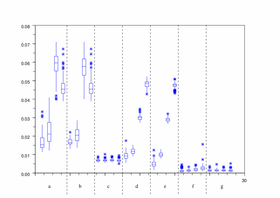
RAND-THRESH-HAAR outperforms ANSCOMBE-UNI and CORRECTED but all these procedures are too rough. To some extent, it is also true for ANSCOMBE-UNI-TI and CORRECTED-TI even if translation invariance improves the corresponding reconstructions. This is not the case for RAND-THRESH-SPLINE and FREE-DEGREE. When $d=70$, performances of all the support-dependent strategies deteriorate, which illustrates the harmful role of the support. In particular, procedures based on the translation invariance principle which periodizes the data, deal with the two main parts of the signal as if they were close to each other, they are consequently quite inadequate. The worse performances of FREE-DEGREE for $d=70$ could be expected since its theoretical performances are established under the strong assumption that the signal is bounded from below on its (known) support. To strengthen these results and to show the influence of the support, we compute the mean square error over 100 simulations for each method and we provide the corresponding boxplots given in Figure 10 associated with $f_{d}$ when $d\in\{10,30,50,70\}.$

Note that when $d$ increases, unlike the other algorithms, performances of our thresholding rule based either on the Haar or on the spline basis are remarkably stable. In particular, for $d=70$, RAND-THRESH-SPLINE outperforms all the other algorithms. Note also the very bad performances of ANSCOMBE-UNI and CORRECTED for $d=50$ due to the inadequacy between the way the data are binned and the distance $d$.

The main conclusions of this short study are the following. We note that the estimate proposed in this paper outperforms ANSCOMBE-UNI and CORRECTED (compare (a), (b) and (c)), showing that the data-driven calibrated threshold proposed in (2.4) improves classical ones. In particular, classical methods highly depend on the way data are binned and on the choice of resolutions levels where coefficients are thresholded, whereas our methodology only depends on $\gamma$ and on $j_{0}$ for which we propose to take systematically $\gamma=1$ and $j_{0}=\log_{2}(n)$. However, unlike FREE-DEGREE, we have to choose a convenient wavelet basis for decomposing the signals. Finally, the support, if too large, can play a harmful role whenever the method needs to rescale the data. This is not the case for the method presented in this paper, which explains the robustness of our procedures with respect to the support issue.

The first point is obvious. For the second point, first, let us take $f\in{\cal F}$. We can write $f=\sum_{\lambda\in\Lambda_{1}}\beta_{\lambda}\tilde{}\varphi_{\lambda}$, where

$$\Lambda_{1}=\{\lambda:\ \beta_{\lambda}\not=0\}$$

is finite. Since $\beta_{\lambda}\not=0$ implies $F_{\lambda}>0$, we have

$$\min_{\lambda\in\Lambda_{1}}F_{\lambda}>0.$$

So, $f$ belongs to ${\cal F}_{n}(R)$ for $n$ and $R$ large enough.
Conversely, if $f=\sum_{\lambda\in\Lambda}\beta_{\lambda}\tilde{}\varphi_{\lambda}$ belongs to ${\mathcal{F}}_{n}(R)$ for some $n$ and some $R>0$ and if $f$ has an infinite number of non-zero wavelet coefficients, then there is an infinite number of indices $\lambda=(j,k)$ such that

$$F_{\lambda}=F_{j,k}\geq\frac{({\log\,}n)({\log\,}{\log\,}n)}{n}.$$

So, either for any arbitrary large $j$, there exists $k$ such that

$$\frac{({\log\,}n)({\log\,}{\log\,}n)}{n}\leq F_{j,k}\leq|\!|f|\!|_{\infty}|\mbox{supp}(\varphi_{j,k})|=|\!|f|\!|_{\infty}2^{-j},$$

so $f\not\in\mathbb{L}_{\infty}(R)$ or there exists $j$ such that $\sum_{k}F_{j,k}=+\infty$ and $f\not\in\mathbb{L}_{1}(R)$ (see (7.5)). This cannot occur since $f\in{\mathcal{F}}_{n}(R)$. This concludes the proof of Proposition 1.

We first state the following lemma established in [23] where it is used to derive Theorem 1. For the sake of exhaustiveness, the proof of Lemma 1 is recalled in section 7.3.

First, we give an upper bound for $\mathbb{E}(\eta_{\lambda,\gamma}^{2})$. For any $\delta>0$,

$$\mathbb{E}(\eta_{\lambda,\gamma}^{2})\leq(1+\delta)2\gamma{\log\,}n\mathbb{E}(\tilde{V}_{\lambda,n})+(1+\delta^{-1})\left(\frac{\gamma{\log\,}n}{3n}\right)^{2}|\!|\varphi_{\lambda}|\!|_{\infty}^{2}.$$

Moreover,

$$\mathbb{E}(\tilde{V}_{\lambda,n})\leq(1+\delta)V_{\lambda,n}+(1+\delta^{-1})3\gamma{\log\,}n\frac{|\!|\varphi_{\lambda}|\!|_{\infty}^{2}}{n^{2}}.$$

So,

$$\mathbb{E}(\eta_{\lambda,\gamma}^{2})\leq(1+\delta)^{2}2\gamma{\log\,}nV_{\lambda,n}+\Delta(\delta)\left(\frac{\gamma{\log\,}n}{n}\right)^{2}|\!|\varphi_{\lambda}|\!|_{\infty}^{2},$$

(6.1)

with $\Delta(\delta)$ a constant depending only on $\delta$. Now, let us choose the parameter $\gamma$ in an optimal way. The main terms in the upper bound given by the lemma are the first and third ones. So, we choose $\kappa^{2}$ close to $\gamma^{-1}$ as required by the assumptions to the lemma and we fix $\gamma$ such that

$$\left(\frac{1+\kappa^{2}}{1-\kappa^{2}}\right)^{2}\approx\left(\frac{\gamma+1}{\gamma-1}\right)^{2}\quad\mbox{and}\quad 2\gamma\left(\frac{1+\kappa^{2}}{1-\kappa^{2}}\right)\approx\frac{2(\gamma^{2}+\gamma)}{\gamma-1}$$

are as small as possible. We first minimize $\frac{2(\gamma^{2}+\gamma)}{\gamma-1}$ so we choose $\gamma=1+\sqrt{2}$. Now, we set $\kappa=\sqrt{0.42}\approx(1+\sqrt{2})^{-1/2}$. Then, with $\delta>0$ such that

$$(1+\delta)^{2}=11.822(1-\kappa^{2})(2\gamma(1+\kappa^{2}))^{-1}\simeq 1.00006,$$

we obtain

$\displaystyle\mathbb{E}|\!|\tilde{f}_{n,\gamma}^{H}-f|\!|_{2}^{2}$

$\displaystyle\leq$

$\displaystyle\inf_{m\subset\Gamma_{n}}\left\{6\sum_{\lambda\not\in m}\beta_{\lambda}^{2}+\sum_{\lambda\in m}(3.4+11.822{\log\,}n)V_{\lambda,n}+\Delta^{\prime}\sum_{\lambda\in m}\left(\frac{{\log\,}n|\!|\varphi_{\lambda}|\!|_{\infty}}{n}\right)^{2}\right\}+\frac{K}{n},$

where

$$\Delta^{\prime}=\Delta(\delta)\gamma^{2}(1+\kappa^{2})(1-\kappa^{2})^{-1}.$$

Let $n$ and $R>0$ be fixed and let $f\in{\cal F}_{n}(R)$. Assume that $\beta_{\lambda}\not=0$. In this case,

$$F_{\lambda}\geq\frac{({\log\,}n)({\log\,}{\log\,}n)}{n}.$$

But

$$F_{\lambda}\leq 2^{-\max(j,0)}|\!|f|\!|_{\infty}\leq 2^{-\max(j,0)}R$$

for $\lambda=(j,k)$. So $2^{j}\leq 2^{j_{0}}$ holds for $n$ large enough and $\lambda$ belongs to $\Gamma_{n}$. Finally, we conclude that $\beta_{\lambda}\not=0$ implies $\lambda\in\Gamma_{n}$. Now, take

$$m=\{\lambda\in\Gamma_{n}:\quad\beta_{\lambda}^{2}>V_{\lambda,n}\}.$$

If $m$ is empty, then $\beta_{\lambda}^{2}=\min(\beta_{\lambda}^{2},V_{\lambda,n})$ for every $\lambda\in\Gamma_{n}$. Hence

$$\mathbb{E}|\!|\tilde{f}_{n,\gamma}^{H}-f|\!|_{2}^{2}\leq 6\sum_{\lambda\in\Gamma_{n}}\min(\beta_{\lambda}^{2},V_{\lambda,n})+\frac{K}{n}$$

and Theorem 2 is proved. If $m$ is not empty, with $\lambda=(j,k)$,

$$V_{\lambda,n}=\frac{2^{\max(j,0)}F_{\lambda}}{n}=\frac{|\!|\varphi_{\lambda}|\!|_{\infty}^{2}F_{\lambda}}{n}.$$

Hence, for all $n$, if $\lambda\in m$, then $\beta_{\lambda}\not=0$ and

$$V_{\lambda,n}{\log\,}n\geq\frac{({\log\,}n)^{2}({\log\,}{\log\,}n)|\!|\varphi_{\lambda}|\!|_{\infty}^{2}}{n^{2}}$$

and if $n$ is large enough,

$$0.1\,{\log\,}n\sum_{\lambda\in m}V_{\lambda,n}\geq\Delta^{\prime}\sum_{\lambda\in m}\left(\frac{{\log\,}n|\!|\varphi_{\lambda}|\!|_{\infty}}{n}\right)^{2}+3.4\sum_{\lambda\in m}V_{\lambda,n}.$$

Theorem 2 is proved since for $n$ large enough (that depends on $R$), we obtain:

$$\mathbb{E}|\!|\tilde{f}_{n,\gamma}^{H}-f|\!|_{2}^{2}\leq 6\sum_{\lambda\not\in m}\beta_{\lambda}^{2}+11.922\,{\log\,}n\sum_{\lambda\in m}V_{\lambda,n}+\frac{K}{n}\leq 12\,{\log\,}n\left(\sum_{\lambda\not\in m}\beta_{\lambda}^{2}+\sum_{\lambda\in m}V_{\lambda,n}+\frac{1}{n}\right).$$

References

• [1] Allen, D.M. (1974). The relationship between variable selection and data augmentation and a method for prediction. Technometrics 16 125–127.
• [2] Arlot, S. and Massart, P. (2009). Data-driven calibration of penalties for least-squares regression. Journal of Machine Learning Research 10 245–279.
• [3] Anscombe, F.J. (1948). The transformation of Poisson, binomial and negative binomial data. Biometrika 35 246–254.
• [4] Autin, F. (2006). Maxiset for density estimation on ℝ\mathbb{R}. Math. Methods Statist 15(2) 123–145.
• [5] Baraud, Y. and Birgé, L. (2006). Estimating the intensity of a random measure by histogram type estimators. Technical report. To appear in Probab. Theory Related Fields.
• [6] Baraud, Y., Giraud, C. and Huet, S. (2008). Gaussian model selection with unknown variance. Technical report. To appear in Annals of Statistics.
• [7] Besbeas, P., De Feis, I. and Sapatinas, T. (2002). A Comparative Simulation Study of Wavelet Shrinkage Estimators For Poisson Counts. Technical report.
• [8] Birgé, L. (2006). Model selection for Poisson processes. Technical report.
• [9] Birgé, L. and Massart, P. (2007). Minimal penalties for Gaussian model selection. Probab. Theory Related Fields 138(1-2) 33–73.
• [10] Cavalier, L. and Koo, J.Y. (2002). Poisson intensity estimation for tomographic data using a wavelet shrinkage approach. IEEE Trans. Inform. Theory 48(10) 2794–2802.
• [11] Cohen, A., Daubechies, I. and Feauveau, J.C. (1992). Biorthogonal bases of compactly supported wavelets. Comm. Pure Appl. Math. 45(5) 485–560.
• [12] Donoho, D.L. (1994). Smooth wavelet decompositions with blocky coefficient kernels. Recent advances in wavelet analysis, Wavelet Anal. Appl. 3 Academic Press, Boston, MA 259–308.
• [13] Donoho, D.L. and Johnstone, I.M. (1994). Ideal spatial adaptation by wavelet shrinkage. Biometrika 81(3) 425–455.
• [14] Donoho, D.L., Johnstone, I.M., Kerkyacharian G. and Picard D. (1996). Density estimation by wavelet thresholding. Annals of Statistics 24(2) 508–539.
• [15] Geisser, S. (1975). The predictive sample reuse method with applications. J. Amer. Statist. Assoc. 70 320–328.
• [16] Johnson, W.B. (1985). Best Constants in Moment Inequalities for Linear Combinations of Independent and Exchangeable Random Variables. Annals of Probability 13(1) 234–253.
• [17] Juditsky, A. and Lambert-Lacroix, S. (2004). On minimax density estimation on ℝ\mathbb{R}. Bernoulli 10(2) 187–220.
• [18] Kingman, J.F.C. (1993). Poisson processes. Oxford studies in Probability.
• [19] Kolaczyk, E.D. (1997). Non-Parametric Estimation of Gamma-Ray Burst Intensities Using Haar Wavelets. The Astrophysical Journal 483 340–349.
• [20] Kolaczyk, E.D. (1999). Wavelet shrinkage estimation of certain Poisson intensity signals using corrected thresholds. Statist. Sinica 9(1) 119–135.
• [21] Lebarbier, E. (2005). Detecting multiple change-points in the mean of Gaussian process by model selection. Signal Processing 85(4) 717–736.
• [22] Reynaud-Bouret, P. (2003). Adaptive estimation of the intensity of inhomogeneous Poisson processes via concentration inequalities. Probability Theory and Related Fields 126(1) 103–153.
• [23] Reynaud-Bouret, P. and Rivoirard, V. (2008). Near optimal thresholding estimation of a Poisson intensity on the real line. Technical report. http://arxiv.org/abs/0810.5204
• [24] Rudemo, M. (1982). Empirical choice of histograms and density estimators. Scand. J. Statist. 9(2) 65–78.
• [25] Stone, M. (1974). Cross-Validatory Choice and Assessment of Statistical Predictions. J. Roy. Stat. Soc., Ser. B 36 111–147.
• [26] Willett, R.M. and Nowak, R.D. (2007). Multiscale Poisson Intensity and Density Estimation. IEEE Transactions on Information Theory 53(9) 3171–3187.