Pulling an adsorbed polymer chain off a solid surface
Abstract
The thermally assisted detachment of a self-avoiding polymer chain from an adhesive surface by an external force applied to one of the chain ends is investigated. We perform our study in the “fixed height” statistical ensemble where one measures the fluctuating force, exerted by the chain on the last monomer when a chain end is kept fixed at height over the solid plane at different adsorption strength . The phase diagram in the plane is derived both analytically and by Monte Carlo simulations. We demonstrate that in the vicinity of the polymer desorption transition a number of properties like fluctuations and probability distribution of various quantities behave differently, if rather than is used as an independent control parameter.
pacs
82.35.Gh Polymers on surface; adhesion - 64.60.A - Specific approaches applied to studies of phase transitions - 62.25.+g Mechanical properties of nanoscale systemsI Introduction
The properties of single polymer chains at surfaces have received considerable attention in recent years. Much of this has been spurred by new experimental techniques such as atomic force microscopy (AFM) and optical/magnetic tweezers [1] which allow one to manipulate single polymer chains. Study of single polymer molecules at surfaces, such as mica or self-assembled monolayers, by Atomic Force Microscopy (AFM) method provides a great scope for experimentation [2, 3, 4, 5, 6, 7, 8]. Applications range from sequential unfolding of collapsed biopolymers over stretching of coiled synthetic polymers to breaking individual covalent bonds[9, 10, 11].
In these experiments it is customary to anchor a polymer molecule with one end to the substrate whereas the other end is fixed on the AFM cantilever. The polymer molecule can be adsorbed on the substrate while the cantilever recedes from the substrate. In so doing one can prescribe the acting force in AFM experiment whereas the distance between the tip and the surface is measured. Conversely, it is also possible to fix the distance and measure the corresponding force, a method which is actually more typical in AFM-experiments. From the standpoint of statistical mechanics these two cases could be qualified as -ensemble (force is fixed while fluctuating the height of the chain end is measured) and as -ensemble ( is fixed while one measures the fluctuating ). Recently these two ways of descriptions as well as their interrelation were discussed for the case of a phantom polymer chain by Skvortsov et al. [12]. In recent papers [13, 14] we studied extensively the desorption of a single tethered self-avoiding polymer from a flat solid substrate with an external force applied to a free chain’s end in the -ensemble.
In the present paper we consider the detachment process of a single self-avoiding polymer chain, keeping the distance between the free chain’s end and the substrate as the control parameter. We derive analytical results for the main observables which characterize the detachment process. The mean value as well as the probability distribution function (PDF) of the order parameter are presented in close analytical expressions using the Grand Canonical Ensemble (GCE) method[14]. The basic force-height relationship which describes the process of polymer detachments by pulling, that is, the relevant equation of state for this system is also derived both for extendible as well as for rigid bonds and shown to comply well with our Monte Carlo simulation results. We demonstrate also that a number of properties behave differently in the vicinity of the phase transition, regarding which of the two equivalent ensembles is used as a basis for the study of systems’s behavior.
II Single chain adsorption: using distance as a control parameter
II.1 Deformation of a tethered chain
Before considering the adsorption-desorption behavior of a polymer in terms of the chain end distance , we first examine how a chain tethered to a solid surface responds to stretching. This problem amounts to finding the chain free end probability distribution function (PDF) where is the chain length, i.e., the number of beads. The partition function of such a chain at fixed distance of the chain end from the anchoring plane is given by
| (1) |
where and the exponent [15]. Here is a model dependent connective constant (see e.g. ref.[15]). In Eq. (1) denotes a short-range characteristic length which depends on the chain model. Below we discuss the chain deformation within two models: the bead-spring (BS) model for elastic bonds and the freely jointed bond vectors (FJBV) model where the bonds between adjacent beads are considered rigid.
II.1.1 Bead-spring model
The form of has been discussed earlier [16, 17] and later used in studies of the monomer density in polymer brushes [18]. Here we outline this in a way which is appropriate for our purposes. The average end-to-end chain distance scales as , where is the mean distance between two successive beads on a chain and is the Flory exponent [19]. The short distance behavior, , is given by
| (2) |
where the exponent . For the long distance behavior, , we assume, following Ref.[18], that the PDF of the end-to-end vector is given by des Cloizeaux’s expression [20] for a chain in the bulk : where the scaling function , and the exponents , . Here and below denotes the space dimensionality. One should emphasize that the presence of a surface is manifested only by the replacement of the universal exponent with another universal exponent (as compared to the pure bulk case!). By integration of over the and coordinates while is measured along the coordinate, one obtains . As the long distance behavior is dominated mainly by the exponential function while the short distance regime is described by Eq. (2), we can approximate the overall behavior as
| (3) |

A comparison of the distribution, Eq. (3), with our simulation data is shown in Fig. 1. The constants and in Eq. (3) can be found from the conditions: and . This leads to:
| (4) |
and
| (5) |
where and . One gets thus the estimates and .
The free energy of the tethered chain with a fixed distance takes on the form where denotes the Boltzmann constant. By making use of Eqs. (1) and (3) the expression for the force , acting on the end-monomer when kept at distance is given by
| (6) |
One should note that at we have which, after taking into account that , leads to the well known Pincus deformation law: [21]. Within the framework of this approximation the (dimensionless) elastic energy reads . In result the corresponding free energy of the chain tail is given by
| (7) |
II.1.2 Freely jointed chain
It is well known [19] that the Pincus law, Eq. (6), describes the deformation of a linear chain at intermediate force strength, . Direct Monte Carlo simulation results indicate that, depending on the model, deviations from Pincus law emerge at (bead-spring off-lattice model) [22], or (Bond Fluctuation Model [23]). In such “overstretched” regime (when the chain is stretched close to its contour length) one should take into account that the chain bonds cannot expand indefinitely. This case could be treated, therefore, within the simple freely jointed bond vectors (FJBV) model [22, 24] where the bond length is fixed. In this model the force - deformation relationship is given by
| (8) |
where denotes the inverse Langevin function and is the fixed bond vector length. We discuss the main results pertaining to the FJBV model in Appendix A. The elastic deformation energy reads , where is the average polar angle of the -th bond vector (see Appendix A). Thus the corresponding free energy of the chain tail for the FJBV model reads
| (9) |
where we have used the notation . Now we are in a position to discuss the pulling of the adsorbed chain controlled by the chain height .
II.2 Pulling controlled by the chain end position
Consider now an adsorbed chain when the adsorption energy per monomer is sufficiently large, , where denotes a corresponding critical energy of adsorption. Below we will also use the notation for the dimensionless adsorption energy. The problem of force-induced polymer desorption could be posed as follows: how is the process of polymer detachment governed by the chain end position ? Figure 2a gives a schematic representation of such a system, and the situation in a computer experiment, as shown in the snapshot Fig. 2b, is very similar.

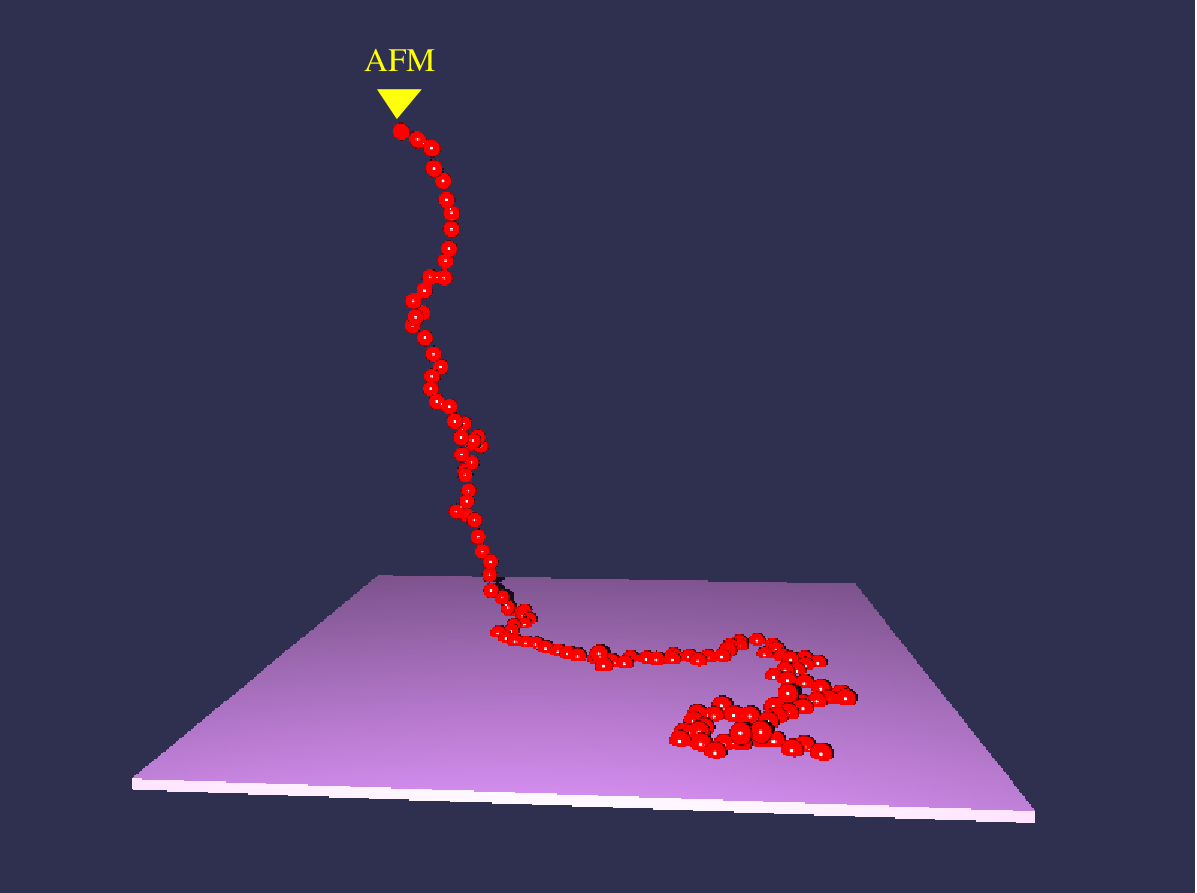
As is evident from Fig. 2a, the system is built up from a tail of length and an adsorbed portion of length . The adsorbed part can be treated within the GCE approach [14]. In our earlier treatment [14] it was shown that the free energy of the adsorbed portion is , where the fugacity per adsorbed monomer depends on and can be found from the basic equation
| (10) |
The so called polylog function in Eq. (10) is defined as and the connective constants , in three and two dimensional space have values which are model dependent [15]. The exponents and where is the crossover exponent which governs the polymer adsorption at criticality, and in particular, the fraction of adsorbed monomers at the critical adsorption point (CAP) . The constant [15]. Finally is the additional statistical weight gained by each adsorbed segment.
In equilibrium, the force conjugated to , that is, , should be equal to the chain resistance force to pulling (where is a scaling function depending only on ), i.e.,
| (11) |
The resisting force holds the last adsorbed monomer on the adhesive plane (see again Fig.2a whereby this monomer is shown to experience a force ). One should emphasize that the force stays constant in the course of the pulling process as long as one monomer, at least, is adsorbed on the surface. Thus corresponds to a plateau on the deformation curve (force vs. chain end position ). The adsorbed monomer (see Fig. 2) has a chemical potential, , which in equilibrium should be equal to the chemical potential of a desorbed monomer in the tail, . The expression for depends on the model and is given either by Eq.(7) for the BS-model or by Eq.(9) in the case of FJBV-model. Taking this into account the condition leads to the following “plateau law” relationship
| (12) |
where stands for the inversion of the function . One should note that Eq.(12) coincides with Eq.(3.16) in Ref. [14] which determines the detachment line in the pulling process controlled by the applied force. Close to the critical point , the plateau force goes to zero. Indeed, since in the vicinity of the critical point (see ref.[14]), and , one may conclude that for the BS-model and for the FJVB-model.
One can solve Eq.(11) with respect to (taking into account that ), and arrive at an expression for the tail length
| (13) |
where the force at the plateau, , is described by Eq. (12). If for the degree of adsorption one uses as an order parameter the fraction of chain contacts with the plane, , where is the number of monomers on the surface, one can write [14]
| (14) |
where and are free energies of the adsorbed and desorbed portions of the chain respectively. The free energy whereas (recall that is the chemical potential of a desorbed monomer). After substitution of these expressions in eq. (14) and taking into account that in equilibrium (the sequence of operations is important: taking the derivative with respect to is to be followed by the condition ) so one gets
| (15) |
i.e. the order parameter is defined by the product of monomer fraction in the adsorbed portion, , and the fraction of surface contacts in this portion, . The expressions for the order parameter can be recast in the form
| (16) |
Here and are some constants of the order of unity.
As one can see from Eq. (16), the order parameter decreases linearly and steadily with . This behavior is qualitatively different from the abrupt jump of when the pulling force is changed as a control parameter. In Section V we will show that this predictions is in a good agreement with our MC - findings. The transition point on the vs. curve corresponds to total detachment, . The corresponding distance will be termed “detachment height” . The dependence of on the adsorption energy can be obtained from Eq.(16) where is set to zero, i.e.
| (17) |
where again as a function of is given by Eq. (12). The line given by Eq. (17), is named “detachment line”. It corresponds to an adsorption - desorption polymer transition which appears as of second order since this order parameter goes to zero continuously as increases. One should emphasize, however, that this “detachment” transition has the same nature as the force-induced desorption transition [14] in the -ensemble where the pulling force , rather than the distance , is fixed and used as a control parameter. This phase transformation is known to be of first order.
III Probability distribution of the number of adsorbed monomers
The grand canonical ensemble (GCE) method, which has been used in our recent paper [14], is a good starting point to calculate the probability distribution function of the adsorbed monomers number . According to this approach, the GCE-partition function of an adsorbed chain has the form
| (18) |
where and are the fugacities conjugated to chain length and to the number of adsorbed monomers , respectively. In Eq.(18) , and denote the GCE partition functions for loops, trains and tails, respectively. The building block adjacent to the tethered chain end corresponds to . It has been shown [14] that the functions , and can be expressed in terms of polylog functions, defined in the paragraph after Eq. (10), as , and , where and are - and - connective constants respectively. By making use of the inverse Laplace transformation of with respect to (see, e.g. [25]) the (canonical with respect to the chain length ) partition function is obtained as
| (19) |
where is a simple pole of in complex -plane given by equation , i.e. by Eq.(10).
The (non-normalized) probability for the chain to have adsorbed monomers is , where is the free energy at given . It is convenient to redefine the fugacity as , (as well as ) where is an arbitrary complex variable. Then the probability can be found as the coefficient of in the function expansion in powers of . Therefore
| (20) |
where the contour of integration is a closed path in the complex plane around . (see e.g. [25]). To estimate the integral in Eq.(20) we use the steepest descent method [25].
For large the main contribution to the integral in Eq. (20) is given by the saddle point of the integrand which is defined by the extremum of the function , i.e., by the condition
| (21) |
The integral is dominated by the term . Another contribution comes from the integration along the steepest descent line. As a result one obtains
| (22) |
The validity of the steepest descent method is ensured by the condition of the second derivative being large, which yields
| (23) |
A more explicit calculation whithin this method can be performed in the vicinity of the critical point .
III.1 PDF of the number of adsorbed monomers close to the critical point of adsorption
In this case the explicit form of is known [14] and after the redefinition of the fugacity, , it reads
| (24) |
where is a constant of the order of unity. The critical adsorption fugacity is defined by the equation
| (25) |
with denoting the Riemann zeta-function.
By using Eq.(24) in Eq.(21) one arrives at the expression for the saddle point
| (26) |
where . Using Eq. (24) and Eq. (26) in Eq. (22) then yields the expression for PDF
| (27) |
For reasonably large and after normalization one arrives at the final expression for the PDF
| (28) |
where we have introduced the usual adsorption scaling variable ( is a constant of the order of unity; see e.g. [26]) as well as the normalization constant :
| (29) |
One can readily see that the width of the distribution increases with or with . To this end one may directly calculate the fluctuation variance as follows:
| (30) |
where the expression for given by Eq.(24) (where also ) has been used. Taking into account that , it becomes clear that the variance really grows with .
The validity of the steepest descent method is ensured by the condition Eq.(23). Using Eq.(24) and Eq. (26), one can verify that this criterion holds when . We recall that , so that . In result the criterion becomes
| (31) |
In the deep adsorption regime this condition might be violated. Nevertheless, the steepest descent method could still be used there, provided that the appropriate solution for (see Eq.(10)) is chosen.
III.2 The regime of deep adsorption
In the deep adsorption regime one should use the the solution for which was also discussed in ref. [14]. Namely, in this case
| (32) |
With Eq. (32) the mean value can be written as
| (33) |
thus tends to with growing as it should be. The variance of the fluctuations within the GCE then becomes
| (34) |
i.e., the fluctuations decrease when the adsorption energy grows. Comparison of this result with the result given by Eq. (30) leads to the important conclusion that the fluctuations of the number of adsorbed monomers first grow with , attain a maximum, and finally decrease with increasing surface adhesion . The position of the maximum reflects the presence of finite-size effects, and, as the chain length , this maximum occurs at the CAP.
Consider now the steepest descent treatment for the deep adsorption regime. With Eq.(32) (after the rescaling ) in Eq.(21), the saddle point becomes
| (35) |
where (recall that ). The main contribution comes from the exponential term in Eq.(22) which is given by
| (36) |
For the expression for the non-normalized PDF takes on the form
| (37) |
where is a constant of the order of unity. Normalization of this distribution yields
| (38) |
where the parameter and the normalization constant
| (39) |
The validity condition, Eq.(23), in the deep adsorption regime (after substitution of Eq. (32) into Eq.(23)) requires
| (40) |
i.e., should not be very close to . In Fig. 3a we show the PDF of the number of chain contacts, , for a free chain without pulling and several adsorption strengths of the substrate. One can readily verify that visually the shape of resembles very much a Gaussian distribution at moderate values of . The PDF variance goes through a sharp maximum at and then declines, as expected from Eq. (34).
One should note that in the -ensemble (where the force and not the distance acts as a controll parameter [14]) the order parameter undergoes a jump at the detachment adsorption energy . This means that . Thus at the detachment point the variance of the fluctuations , which practically means that for chains of a finite length the distribution at becomes very broad, in sharp contrast to Eq. (34). This has indeed been observed in our MC-simulation results (see Fig.12 in ref. [14]).
III.3 distribution in the subcritical regime of underadsorption
In the subcritical regime, , the fraction of adsorbed points (order parameter) , in the thermodynamic limit. Nevertheless, and one can examine the form of the PDF . At the solution for (the simple pole of in the complex -plane) does not exist because (see Eq.(18)). However, the tail GCE-partition function has a branch point at (see Eq. (A 11) in ref. [14]) which governs the coefficient at , i.e., the partition function . The calculation (following Section 2.4.3 in ref. [25]) yields
| (41) |
where and we have also used that at the loop and train GCE-partition functions are and respectively. This expression has a pole at (cf. Eq. (25)) which yields the coefficient of , i.e. . Recall that , so that . Expansion of the denominator in Eq. (41) around reveals the simple pole as follows
| (42) |
In (42) we have used the relationship . The coefficient of , i.e., , is proportional to . Therefore . Taking the normalization condition into account, the final expression for can be recast in the form
| (43) |
i.e., has a simple exponential form. The calculation of the average leads to the simple result , i.e., at . On the other hand we know that at . In order to prevent a divergency at , one should incorporate an appropriate cutoff in the PDF given by Eq.(43). With this the distribution is given by
| (44) |
Thus the expression for the average number of adsorbed monomer has the correct limit behavior, i.e.,
| (45) |
III.4 Probability distribution function in the -ensemble
Eventually we examine how the fixed chain-end hight affects the PDF of the number of contacts . To this end we refer again to Fig. 2a where an adsorbed chain with a fixed height of the last monomer is depicted. The adsorbed chain consists of a tail of length and of an adsorbed part with beads. One should bear in mind that is function of the control parameters and of given by eqs.(12) and (13). The partition function of the adsorbed part is then given by
| (46) |
where we took into account that the free energy of the adsorbed portion is given as (see Sec. II B).

As mentioned above, the PDF , so that by means of rescaling and the PDF can be found as the coefficient of , i.e.,
| (47) |
As before, the steepest descent method can be used to calculate the integral in Eq. (47). However, in this case the calculations are more complicated and we have relegated most of them to Appendix B. As may be seen there, the saddle point equation can not be solved analytically in the general case but could be treated iteratively for relatively small heights .
IV Monte Carlo Simulation Model
We use a coarse grained off-lattice bead-spring model [27] which has proved rather efficient in a number of polymers studies so far. The system consists of a single polymer chain tethered at one end to a flat impenetrable structureless surface. The surface interaction is described by a square well potential,
| (48) |
The strength is varied from to while the interaction range . The effective bonded interaction is described by the FENE (finitely extensible nonlinear elastic) potential:
| (49) |
with , and the fully stretched-, mean-, and minimum bond lengths . The nonbonded interactions between monomers are described by the Morse potential:
| (50) |
with . In few cases, needed to clarify the nature of the polymer chain resistance to stretching, we have taken the nonbonded interactions between monomers as purely repulsive by shifting the Morse potential upward by and removing its attractive branch for .
We employ periodic boundary conditions in the directions and impenetrable walls in the direction. The lengths of the studied polymer chains are typically , and . The size of the simulation box was chosen appropriately to the chain length, so for example, for a chain length of , the box size was . All simulations were carried out for constant position of the last monomer -coordinate, that is, in the fixed height ensemble. The the fluctuating force , exerted on the last bead by the rest of the chain was measured and average over about measurements. The standard Metropolis algorithm was employed to govern the moves with self avoidance automatically incorporated in the potentials. In each Monte Carlo update, a monomer was chosen at random and a random displacement attempted with chosen uniformly from the interval . If the last monomer was displaced in direction, there was an energy cost of due to the pulling force. The transition probability for the attempted move was calculated from the change of the potential energies before and after the move was performed as . As in a standard Metropolis algorithm, the attempted move was accepted, if exceeds a random number uniformly distributed in the interval .
As a rule, the polymer chains have been originally equilibrated in the MC method for a period of about MCS after which typically measurement runs were performed, each of length MCS. The equilibration period and the length of the run were chosen according to the chain length and the values provided here are for the longest chain length.
V Monte Carlo simulation results
In order to verify the theoretical predictions, outlined in Section II, we carried out extensive Monte Carlo simulations with the off-lattice model, defined in Section IV. In these simulations we fix the end monomer of the polymer chain at height above the adsorbing surface, and measure the (fluctuating) force, needed to keep the last bead at distance , as well as the corresponding fraction of adsorbed monomers . These computer experiments are performed at different strengths of the adsorption potential, Eq. (48).


In Figs. 4a,b we compare the predicted dependence of the order parameter on the (dimensionless) height at several values of with the results from MC simulations. Note, that the critical point of adsorption so we take our measurements above the region of critical adsorption. Typically, both in the analytic results, Fig. 4a, and in the MC-data, Fig. 4b, for , one recovers the predicted linear decrease of with growing . Finite-size effects lead to some rounding of the simulation data (in Fig. 4b these effects are seen to be larger for than for ) when so that the height of detachment is determined from the intersection of the tangent to and the axis where

. Evidently, with growing adsorption strength, , larger height is needed to detach the polymer from the substrate. Thus, one may construct a phase diagram for the desorption transition, which we show in Fig. 5. The theoretical prediction is given by eq. (17).
In the insets of Fig. 4a,b we also show the variation of the fraction of adsorbed segments with adsorption strengths for several heights of a chain with . It is evident that, apart from the rounding of the MC data at , one finds again good agreement between the behavior, predicted by Eq. (15), and the simulation results.
The gradual change of in the whole interval of possible variation of suggests a pseudo-continuous phase transition, as pointed out in the end of Section II, Eq. (16). Of course, if is itself expressed in terms of the measured pulling force, one would again find that changes abruptly with varying at some threshold value , indicating a first order transformation from an adsorbed into a desorbed state of the polymer chain.

It has been pointed out earlier by Skvortsov et al.[12] that, while both the fixed-force and the fixed-height ensembles are equivalent as far as the mean values of observables such as the fraction of adsorbed monomers and other related quantities are concerned, this does not apply to some more detailed properties like those involving fluctuations. Therefore, it is interesting to examine the fluctuations of the order parameter, , for different values of our control parameter , and compare them to theoretical predictions for from Section II. First we compare the order parameter distribution for zero force, Fig. 6, obtained from our computer experiment, to that, predicted by Eqs. (28), (38), (44), and displayed in Fig. 3a. It is evident from Fig. 6 that for free chains at different strengths of adhesion there is a perfect agreement between analytical and simulational results. For rather weak adsorption in the subcritical regime, one can verify from Fig. 6 that gradually transforms from nearly Gaussian into exponential distribution, as expected from Eq. (44). For the distribution width grows and goes through a sharp maximum in the vicinity of , and then drops as increases further - compare insets in Fig. 6 and Fig. 3a.


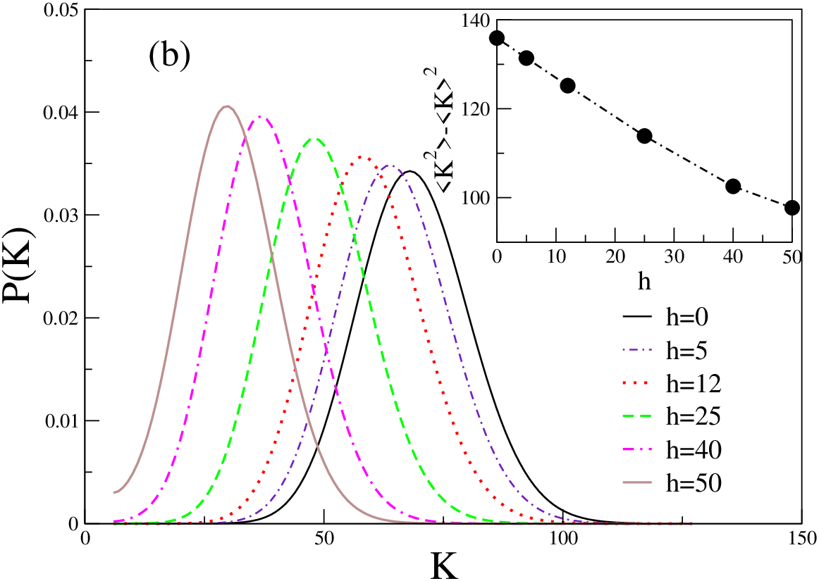
Let us consider now PDF in the presence of pulling. In Fig. 7a we display the distribution measured in the MC simulations for different heights and constant adsorption energy . One can readily verify from our results that far enough from the detachment line, , the shape of looks like Gaussian and that the second moment, , remains unchanged with varying height . Of course, when , the maximum of shifts to lower values of . Only in the immediate vicinity of , where and the fluctuations strongly decrease, one observes a significant deviation from the Gaussian shape - cf. the inset in Fig. 7a. The latter is illustrated in more detail in Fig. 7b where we show the measured variation of the second moment, , and that of the third moment, with increasing height . The deviation from Guassinity in , measured by the deviation of the third moment from zero, is localized in the vicinity of the detachment height . The corresponding theoretical prediction for the relatively weak adsorption strength is depicted in Fig. 3b. It can be seen that with increasing the almost Gaussian distribution tends to Poisson-like one. Also the fluctuations decrease with in accordance with MC-findings.
The force , exerted by the chain on the end-monomer, when the latter is kept at height above the surface, is one of the main properties which can be measured in experiments carried out within the fixed-height ensemble. Note that has the same magnitude and opposite sign, regarding the force, applied by the experimentalist. The variation of the force with increasing height is shown in Fig. 8a for several values of the adsorption potential . In Fig. 8a we distinguish between two contributions to the total force , acting on the end bead. The first stems from the quasi-elastic forces of the bonded interaction (FENE) whereas the second contribution is due to the short-range (attractive) interactions between non-bonded monomers (in our model - the Morse potential). A typical feature of the relationship, namely, the existence of a broad interval of heights where the force remains constant (a plateau in the force) is readily seen in Fig. 8a. With growing strength of adsorption the length of this plateau as well as the magnitude of the plateau force increase. Note, that for no plateau whatsoever is found. Upon further extension (by increasing ) of the chain, the plateau ends and the measured force starts to grow rapidly in magnitude - an effect, caused by a change of the chain conformation itself in the entirely desorbed state.
A closer inspection of Fig. 8a reveals that the non-bonded contribution to , which is generally much weaker than the bonded one, behaves differently, depending on whether the forces between non-nearest neighbors along the backbone of the chain are purely repulsive, or contain an attractive branch. While for strong adsorption, , a plateau is observed even for attractive non-bonded interactions, for weak adsorption, , an increase of the non-bonded contribution at , (seen as a minimum in Fig. 8a) is observed. This effect is entirely missing in the case of purely repulsive nonbonded


interactions - see the inset in Fig. 8a where the contributions from bonded and non-bonded interactions are shown for a neutral surface . If one plots the magnitude of the measured force at the plateau against the corresponding value of the the adsorption potential, , one may check the theoretical result, Eq. (12) - Fig. 8b. Evidently, the theoretical predictions about agree well with the observed variation of the detachment force in the MC simulation, both within the BS- or FJBV models, as long as only the excluded volume interactions in the MC data are taken into account. If the total contribution to , including also attractive non-bonded interactions in the chain, is depicted - black triangles in Fig. 8b - then the agreement with the theoretical curves deteriorates since the latter do not take into account the possible presence of attractive non-bonded interactions.


The relationship, which gives the equation of state of the stretched polymer, may be derived within one of the different theoretical models, e.g., that of BS-, Eq. (6), or FJBV-model, Eq. (8), as mentioned in Section II. Which of these theoretical descriptions is the more adequate can be decided by comparison with experiment. In Fig. 9a,b, we present such comparison by plotting our simulation data using different normalization for the height . From Fig. 9a it becomes evident that the data from our computer experiment for and collapse on a single curve, albeit this collapse only holds as long as for the BS-model while it fails for stronger stretching. In contrast, this collapse works well for all values of , provided the height is scaled with the contour length of the chain , rather than with , as in the FJBV model - Fig. 9b - regardless of whether a purely repulsive, or the full Morse potential (which includes also an attractive part) of interactions is involved. The analytical expression, Eq. (8), is found to provide perfect agreement with the simulation data for strong stretching, . From the simulation data on Fig. 9 one may even verify that the force goes through zero at some height and then turns negative, provided one keeps the chain end very close to the grafting surface (cf. eq.(6)).
VI Summary
In the present work we have treated the force-induced desorption of a self-avoiding polymer chain from a flat structureless substrate both theoretically and by means of Monte Carlo simulation within the constant-height ensemble. The motivation for this investigation has been the necessity to distinguish between results obtained in this ensemble and results, derived in the constant-force ensemble, considered recently[14], as far as both ensembles could in principle be used by experimentalists. We demonstrate that the observed behavior of the main quantity of interest, namely, the fraction of adsorbed beads (i.e., the order parameter of the phase transition) with changing height differs qualitatively from the variation of the order parameter when the pulling force is varied. In the constant-height ensemble one observes a steady variation of with changing whereas in the constant-force ensemble one sees an abrupt jump of at a particular value of , termed a detachment force. However, this should not cast doubts on the genuine first-order nature of the phase transition which can be recovered within the constant-height ensemble too, provided one expresses the control parameter in terms of the average force . This equivalence has been studied extensively for Gaussian chains by Skvortsov et al. [12] who noted that ensemble equivalence does not apply to fluctuations of the pertinent quantities too.
Indeed, in our earlier study[13] we found diverging variance of the PDF at whereas in our present study the fluctuations of the order parameter are observed to stay finite at the transition height . These findings confirm theoretical predictions based on analytic results which we derive within the GCE-approach. Within this approach we have explored two different theoretical models for the basic force - extension relationship, namely, the bead-spring (BS) model as well as that of a Freely-Jointed Bond-Vectors (FJBV) model. Our simulation results indicate a good agreement between theory and computer experiment.
Acknowledgments
We are indebted to A. Skvortsov for useful discussions during the preparation of this work. A. Milchev thanks the Max-Planck Institute for Polymer Research in Mainz, Germany, for hospitality during his visit at the institute. A. Milchev and V. Rostiashvili acknowledge support from the Deutsche Forschungsgemeinschaft (DFG), grant No. SFB 625/B4.
Appendix A Freely jointed bond vectors model
The deformation law in the overstretched regime (when the chain deformation is close to its saturation) could be treated better within the FJBV model. Consider a tethered chain of length with one end anchored at the origin of the coordinates and an external force acting on the free end of the chain. The corresponding deformation energy reads
| (51) |
where is the -coordinate (directed perpendicular to the surf ace) of the chain end, and are the length and the polar angle of the -th bond vector respectively. The corresponding partition function of the FJBV model is given by
| (52) | |||||
The average orientation of the -th bond vector can be calculated as
| (53) |
From Eq.(53) the chain end mean distance from the surface, , is given by
| (54) |
where we have taken into account that the lengths of all bond vectors are of equal length, , and is the Langevin function. This leads to the force - distance relationship
| (55) |
which we use in Sec.II. The notation stands for the inverse Langevin function.
Appendix B Calculation of PDF in the -ensemble
Using Eq.(24) for as well as Eqs. (12) and (13) (for the BS-model), one obtains an expression for the tail length
| (56) |
The saddle point (SP) equation in this case reads (cf. Eq.(21))
| (57) |
Taking into account Eqs. (24) and (56), after introducing the notation , the SP-equation can be recast into
| (58) |
where and are constants of the order of unity. In the particular case Eq.(58) goes back, as expected, to Eq.(26). Eq. (58) can be solved iteratively for as
| (59) |
As before, the main contribution in the integral given by Eq. (47) reads
| (60) | |||||
where one introduces the notation
| (61) |
After normalization, the final expression for the PDF reads
| (62) |
where as before and the normalization constant reads
| (63) |
Again one can readily see that for Eq.(62) reduces to Eq.(28). The PDF, following from Eq. (62) is shown in Fig. 3b for several values of the height . Evidently, both the mean value and the variance decline with growing .
References
- [1] S. B. Smith, Y. Cui, and C. Bustamante, Science 271, 795(1996).
- [2] T. J. Senden, J.-M. di Meglio, and P. Auroy, Europ. Phys. J. B3, 211(1998).
- [3] T. Hugel, M. Grosholz, H. Clausen-Schaumann, A. Pfau, H. E. Gaub, and M. Seitz, Macromolecules, 34, 1039(2001)
- [4] H. Hugel, M. Seitz, Macromol. Rapid. Commun. 22, 989 (2001).
- [5] A. Rohrbach, E.H.K. Stelzer, J. Appl. Phys. 91, 5474 (2002).
- [6] L. Sonnenberg, Y. Luo, H. Schaad, M. Seitz, H. Gölfen, H.E. Gaub, J. Am. Chem. Soc. 129, 15364 (2007).
- [7] C. Friedsam, A. Del Campo Becares, M. Seitz, and H. E. Gaub, New J. Phys. 6, 9(2004).
- [8] S.K. Kufer, E.M. Puchner, H. Gumpp, T. Liedl, H.E. Gaub, Science, 319, 594 (2008).
- [9] M. Rief, F. Oesterhelt, B. Heymann, and H. E. Gaub, Science 275, 1295(1997).
- [10] C. Ortiz and G. Hadziioannou, Macromolecules 32, 780(1990).
- [11] M. Grandbois, M. Beyer, M. Rief, H. Clausen-Schaumann, and H. E. Gaub, Science 283, 1727(1999).
- [12] A.M. Skvortsov, L.I. Klushin, T.M. Birshtein, Polymer Sci. (Moscow) Ser. A, 51, 1 (2009).
- [13] S. Bhattacharya, V.G. Rostiashvili, A. Milchev, T.A. Vilgis, Phys. Rev. E 79, 030802(R) (2009).
- [14] S. Bhattacharya, V.G. Rostiashvili, A. Milchev, T.A. Vilgis, Macromolecules, 42, 2236 (2009).
- [15] C. Vanderzande, Lattice Model of Polymers, Cambridge University Press, Cambridge, 1998.
- [16] E. Eisenriegler, K. Kremer, K. Binder, J. Chem. Phys. 77, 6296 (1982).
- [17] E. Eisenriegler, Polymers Near Surfaces, World Scientific, 1993.
- [18] T. Kreer, S. Metzger, M. Müller, K. Binder, J. Chem. Phys. 120, 4012 (2004).
- [19] A.Yu. Grosberg, A.R. Khokhlov,Statistical Physics of Macromolecules (AIP, New York, 1994).
- [20] J. des Cloiseaus, G. Jannink, Polymers in Solution, Clarendon Press, Oxford, 1990.
- [21] P.-G. de Gennes, Scaling Consept in Polymer Physics, Cornell Univercity Press, 1979.
- [22] Y.-J. Sheng, P.-Y. Lai, Phys. Rev. E 56, 1900 (1997).
- [23] M. Wittkop, J.-U. Sommer, S. Kreitmeier, D. Göritz, Phys. Rev. E 49, 5472 (1994).
- [24] J.U. Schurr, S.B. Smith, Biopolymers, 29, 1161 (1990).
- [25] J. Rudnick, G. Gaspari, Elements of Random Walk, Cambridge Univercity Press, Cambridge, 2004.
- [26] S. Bhattacharya, H.-P. Hsu, V.G. Rostiashvili, A. Milchev, T.A. Vilgis, Macromolecules, 41, 2920 (2008).
- [27] K. Binder and A. Milchev, J. Computer-Aided Material Design, 9, 33(2002)