The transient and the late time attractor tachyon dark energy: Can we distinguish it from quintessence ?
Abstract
The string inspired tachyon field can serve as a candidate of dark energy. Its equation of state parameter varies from to . In case of tachyon field potential slower(faster) than at infinity, dark energy(dark matter) is a late time attractor. We investigate the tachyon dark energy models under the assumption that is close to . We find that all the models exhibit unique behavior around the present epoch which is exactly same as that of the thawing quintessence.
I Introduction
One of the most challenging problems of modern cosmology is associated with late time acceleration of universe which is supported by observations of complementary nature. According to the standard lore, an exotic perfect barotropic fluid with large negative pressure dubbed dark energy can account for repulsive effect causing acceleration[1, 2, 3]. The simplest example of dark energy is provided by cosmological constant . The model is consistent with observation but is plagued with difficult theoretical issues. The field theoretic understanding of is far from being satisfactory and its small numerical values gives rise to problems of fine tuning and coincidence. A variety of scalar field models including quintessence, tachyons, phantoms and K-essence has been investigated in the recent years to address the problem[2, 4, 5]. These models have some advantage over the cosmological constant: (i) They can mimic cosmological constant at the present epoch and can give rise to other observed values of the equation of state parameter (recent data indicate that lies in a narrow strip around and is consistent with being below this value). (ii) They can alleviate the fine tuning and coincidence problems.
The scalar field model, which is the simplest generalization of cosmological constant, is one with a linear potential [6]. This model starts with a cosmological constant like behaviour where the scalar field is frozen initially due to Hubble damping. Later on, it starts rolling, but because the potential has no minimum, it leads to a collapsing universe in future. Hence universe in this model, has a finite history.
The more complicated scalar field models can broadly be classified into two categories. Models in which scalar field mimics the background (radiation/matter) being subdominant for most of the evolution history. Only at late times it becomes dominant and accounts for the late time acceleration. Such a solution is referred to as tracker. In this case () before the transition from matter like regime or scaling regime to accelerated expansion. Tracker models are independent of initial conditions used for field evolution but do require the tuning of the slope of the scalar field potential. During the scaling regime the field energy density is of the same order of magnitude as the background energy density.
In second class of models, trackers are absent. Hence at early times, the field gets locked () due to large Hubble damping and waits for the matter energy density to become comparable to field energy density which is made to happen at late times. The field then begins to evolve towards larger values of starting from . In this case, for a viable cosmic evolution, one chooses during the locking regime which requires the tuning of initial conditions of the field. The two classes of scalar fields are called Freezing and Thawing models.
In case of standard scalar field (quintessence), there is a variety of models which possess tracker solutions. In case of tachyon field[7, 8] (motivated by string theory), there exists no solution which can mimic scaling matter/radiation regime[9, 10, 11, 12, 13, 14, 15, 16, 17]. These models necessarily belong to the class of thawing models. Tachyon models do admit scaling solution in presence of a hypothetical barotropic fluid with negative equation of state. Tachyon fields can be classified by the asymptotic behavior of their potentials for large values of the field: (i) faster than for . In this case dark matter like solution is a late time attractor. Dark energy may arise in this case as a transient phenomenon. (ii) slower than for ; these models give rise to dark energy as late time attractor. The two classes are separated by which is scaling potential with .
Since observationally, the equation of state parameter of dark energy is very close to one, we can use this information to simplify the dynamics. In case of thawing quintessence and phantom field, it allows to obtain a generic expression for which represents the entire class of quintessence and phantom models[18, 19]. In this paper we apply the same technique to tachyon field which belongs to the class of thawing models. With the current state of observation, we address the issue of distinguishing the tachyon dark energy from the case of quintessence.
II Dynamics of tachyon field
In what follows we shall be interested in the cosmological dynamics of tachyon field which is specified by the Dirac-Born-Infeld (DBI) type of action given by
| (1) |
where on phenomenological grounds, we shall consider a wider class of potentials satisfying the restriction that as . The parameter where the plus sign corresponds to the normal tachyon field which is non-phantom whereas with minus sign, one can model phantom type tachyon fields phenomenologically. In FRW background, the pressure and energy density of are given by
| (2) |
| (3) |
The equation of motion which follows from (1) is
| (4) |
where is the Hubble parameter
| (5) |
The evolution equation can be cast in the following autonomous form for the convenient use
| (6) | |||
| (7) | |||
| (8) |
with
| (9) |
where prime denotes the derivative with respect to . Here is defined as for the background field. In our subsequent calculations, we shall assume a non-relativistic matter for our background field for which .
An important remark on the autonomous system is in order. Let us consider the inverse power law type potential . Eq.(9) tells us that if allowing to increase monotonously for large values of the field. In this case or where as approaches the de-Sitter limit for (). These two classes of tachyon potentials are separated by the inverse square potential with constant () which provides the analog of scaling potential in case of tachyon. However, there is major difference that in the present case, the field can only mimic a hypothetical fluid with negative equation of state leading to accelerated expansion. Unfortunately, the mass scale in the potential turns out be larger than the Planck mass. The class of potentials designated by is free from this problem and gives rise to dark energy as late time attractor of dynamics.

In the analysis to follow, it will be convenient to use the following quantities
| (10) |
where is the equation of state for the tachyon field. One can now express the autonomous equations through them:
| (11) |
| (12) |
| (13) |
The first two equations can be combined into one by a change of variable from
| (14) |
II.1 Late time evolution
From Eq.(14), one can see that for non-phantom and phantom cases, i.e , the equation is completely different and hence one expects to have different evolutions for for non-phantom and phantom cases.

But we are interested in the investigations of cosmological dynamics around the present epoch where . Secondly, in our case improves slightly beginning from the locking regime, thereby, telling us that the slope of the potential does not change appreciably. This implies that the potential is very flat around the present epoch such that
| (15) |

In case of field domination regime, the two conditions in Eq.(15) define the slow roll parameters which allows to neglect the term in equation of motion for . In the present context, unlike the case of inflation, the evolution of field begins in the matter dominated regime and even today, the contribution of matter is not negligible. The traditional slow roll parameters can not be connected to the conditions on slope and curvature of potential which essentially requires that Hubble expansion is determined by the field energy density alone. Thus the slow roll parameters are not that useful in case of late time acceleration, though, Eq.(15) can still be helpful.

In view of the aforesaid, we can drop all the terms of order higher than in Eq.(14)and assume that the slope of the potential is constant, . These follow from the two slow-roll conditions (15) as we shall show later. Evolution equation then simplifies to
| (16) |
Let us note that Eq.(16) is same as its counter part in case of quintessence though the full Eq.(14) is different. The difference between tachyon and quintessence dynamics is represented by terms of higher order than . Thus if we restrict our investigation of dark energy dynamics very close to cosmological constant behavior, we can not distinguish tachyon dark energy from quintessence. Also equation (16) is independent of . Hence for non-phantom case and for phantom case, have exactly similar evolution around cosmological constant.
Eq.(16) can be transformed into a linear differential
equation with the change of variable ,
we have boundary condition at .
The resulting solution expressed in terms of
| (17) |
Under the approximation which is justified about the present epoch, all the tachyon models follow a general track irrespective of the particular field potential. One can see from (17) that . Hence the first slow roll condition () ensures that . We can quantify our second assumption that the slope of the potential does not change appreciably during the evolution as . Noting that and also , one can then use eqn (13) to write
| (18) |
together with the first slow-roll condition, this ensures the second slow-roll condition to be satisfied. We also show in figure 5, the actual behavior of for different potentials for non-phantom case. This also shows is constant during the entire evolution for all practical purposes. One can also arrives the same behavior for phantom case. In figure 1 and figure 3, we show the our analytical approximation for in comparison with the numerical solutions of the exact equations for different potentials with different initial values for for non-phantom and phantom cases. They show that our approximation works reasonably well as long as is small, i.e as long as the slow-roll conditions are satisfied.
Next, we can use eqn (12) to solve for to determine . assuming , this gives
| (19) |
where is the present day value of . Equation (17) and (19) gives the complete behavior for the equation of state for tachyon fields with potentials satisfying the slow-roll conditions (15). One can also express the parameter in terms of the present day value of the equation of state which is quite straightforward. This behaviours are shown in figure 2 and figure 4 for non-phantom and phantom cases.
Similar to the case of thawing quintessence, non-phantom tachyon models are restricted to a part of the plane. To specify the the limits, let us define a parameter
Since the Hubble parameter is determined by matter dominated regime in the beginning of evolution, we find that as which leads to the upper limit, . The lower bound on is estimated numerically (demanding that at present ) as, giving rise to the permissible region of - plane
| (20) |
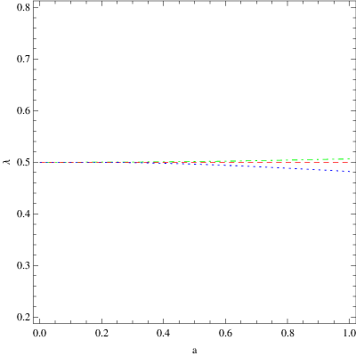
In figure 3 we have shown this permissible region together with the actual behavior for different potentials.

III Observational Constraint
The solution given by Eqs.(17) (19) for the equation of state parameter versus the scale factor for tachyon field under slow-roll conditions is exactly similar to that for a canonical scalar field as obtained earlier in [18, 19]. They have also constrained the two parameters and of the model using the SNLS (Supernva Legacy Survey)[20] and BAO data[21]. At present, we have the Union08 compilation of the SnIa data which contains around 307 data points[22]. This is world’s published first heterogeneous SN data set containing large sample of data from SNLS, Essence survey, high redshift supernova data from Hubble Space telescope as well as several small data sets. We use this data set together with the BAO data from SDSS (Sloan Digital Sky Survey)[21]. The and contour intervals for our model have been shown in figure 4. From the figure, it is clear that one can not distinguish cosmological constant with a thawing dark energy models with present data although the phantom dark energy models are preferred.

IV Conclusions
In this paper we have examined the DBI system with a phenomenologically motivated class of run away potentials. In general, the the tachyon dynamics crucially depends upon the asymptotic behavior of the potential at large values of . The inverse square potential gives rise to constant equation of state which is determined by the slope of the potential, . We analysed the class of tachyon potentials with dark energy and dark matter as late time attractors. Models in which decrease faster than can give rise to transient dark energy near the top of the potential and then mimic dark matter as late time attractor. Since for tachyon field scales slower than matter, its energy density for a viable cosmic evolution should be fixed around at earlier epochs allowing the field to freeze due to large Hubble damping. Thus all the three classes of tachyon models belong to thawing type. The data available at present allows to carry out investigations around the present epoch with . As soon as becomes, comparable to matter density, field begins evolve. The equation of state improves slightly starting from . Hence, the slope of the potential does not change appreciably which we confirmed numerically. In the limit of small adiabatic index of assuming to be constant, we have shown that the resulting evolution equations are same as in case of quintessence which can be solved analytically. Our simulation shows that the approximation is very close to the numerical results for around the present epoch. Deviations are possible in the far future. We therefore conclude that tachyon dynamics is difficult to distinguish from quintessence at least in the near future. We also extended our analysis to the case of phantom tachyon. Again in the region of interest, we find that phantom tachyon model is difficult to distinguish from the ordinary phantom field. We also constrained the parameters and for our model using the latest supernovae data along with baryon acoustic oscillation BAO data. Our analysis shows some preference for phantom energy.
The fact that all the scalar field dark energy models have a unique equation of state as long as they are in the slow-roll regime, makes a strong case for the given by equations (17) and (19). It does not matter whether the scalar field has a canonical or non-canonical kinetic term. It is also the same for non-phantom or phantom scalar fields. We hope that this equation of state behaviour for the dark energy will be considered seriously while fitting with the observational data coming from future experiments.
V Acknowledgemnet
AAS acknowledges the financial support provided by the University Grants Commission, Govt. Of India, through the major research project grant (Grant No: 33-28/2007(SR)).
References
- [1] V. Sahni and A. A. Starobinsky, Int. J. Mod. Phys. D 9, 373 (2000); S. M. Carroll, arXiv:astro-ph/0004075; T. Padmanabhan, Phys. Rept. 380, 235(2003); P. J. E. Peebles and B. Ratra, Rev. Mod. Phys. 75, 559 (2003); E. V. Linder, arXiv:astro-ph/0511197; 1753(2006)[hep-th/0603057]; L. Perivolaropoulos, astro-ph/0601014; N. Straumann, arXiv:gr-qc/0311083.
- [2] E. J. Copeland, M. Sami and S. Tsujikawa, Int. J. Mod. Phys., D15 , 1753(2006)[hep-th/0603057].
- [3] E. V. Linder, astro-ph/0704.2064; J. Frieman, M. Turner and D. Huterer, arXiv:0803.0982; Robert R. Caldwell and Marc Kamionkowski,arXiv:0903.0866; A. Silvestri and Mark Trodden, arXiv:0904.0024.
- [4] I. Zlatev, L. M. Wang and P. J. Steinhardt, Phys. Rev. Lett. 82, 896 (1999); P. J. Steinhardt, L. M. Wang and I. Zlatev, Phys. Rev. D 59, 123504 (1999); L. Amendola, Phys. Rev. D 62, 043511 (2000).
- [5] C. Armendariz-Picon, V. Mukhanov and P. J. Steinhardt, Phys. Rev. Lett. 85, 4438 (2000); Phys. Rev. D 63, 103510 (2001); T. Chiba, T. Okabe and M. Yamaguchi, Phys. Rev. D 62, 023511 (2000).
- [6] R. Kallosh, J. Kratochvil, A. Linde, E. Linder and M. Shmakova, JCAP 0310, 015 (2003); R. Kallosh, J. Kratochvil, A. Linde, E. Linder and M. Shmakova, JCAP 0412, 006 (2004); P. P. Avelino, C. J. A. P . Martins, and J. C. R. E. Oliveira Phys. Rev. D 70, 083506 (2004); P. P. Avelino Phys. Lett. B. 611, 15 (2005).
- [7] A. Sen, JHEP 0204, 048 (2002); JHEP 0207, 065 (2002); Mod. Phys. Lett. A 17, 1797 (2002); arXiv: hep-th/0312153.
- [8] A. Sen, JHEP 9910, 008 (1999); M. R. Garousi, Nucl. Phys. B584, 284 (2000); Nucl. Phys. B 647, 117 (2002); JHEP 0305, 058 (2003); E. A. Bergshoeff, M. de Roo, T. C. de Wit, E. Eyras, S. Panda, JHEP 0005, 009 (2000); J. Kluson, Phys. Rev. D 62, 126003 (2000); D. Kutasov and V. Niarchos, Nucl. Phys. B 666, 56 (2003).
- [9] E. J. Copeland, M. R. Garousi, M. Sami , S. Tsujikawa, Phys. Rev. D71, 043003 (2005)[hep-th/0411192].
- [10] S. Tsujikawa and M. Sami, Phys. Lett. B603, 113(2004)[hep-th/0409212]; M. Sami, N. Savchenko and A. Toporensky, Phys. Rev. D70, 123528(2004)[hep-th/0408140].
- [11] L. P. Chimento, Monica Forte, G. M. Kremer and M. O. Ribas, 0809.1919 [gr-qc]; W. Chakraborty, Ujjal Debnath, e-Print: arXiv:0804.4801; I.Ya. Aref’eva and A.S. Koshelev, JHEP 0809:068,2008[0804.3570]; Zong-Kuan Guo and Nobuyoshi Ohta, JCAP 0804:035,2008; M.R. Setare, Phys. Lett. B653, 116(2007); Z. Keresztes, L.A. Gergely, V. Gorini, U. Moschella, A.Yu. Kamenshchik, arXiv:0901.2292.
- [12] T. Padmanabhan, Phys. Rev. D 66, 021301 (2002).
- [13] G. N. Felder, Lev Kofman and A. Starobinsky,JHEP 0209,026(2002)[hep-th/0208019]
- [14] J. S. Bagla, H. K. Jassal and T. Padmanabhan, Phys. Rev. D 67, 063504 (2003).
- [15] L. R. W. Abramo and F. Finelli, Phys. Lett. B 575 (2003) 165.
- [16] J. M. Aguirregabiria and R. Lazkoz, Phys. Rev. D 69, 123502 (2004).
- [17] Z. K. Guo and Y. Z. Zhang, JCAP 0408, 010 (2004).
- [18] R. J. Scherrer and A. A. Sen, Phys. Rev. D 77, 083515 (2008).
- [19] R. J. Scherrer and A. A. Sen, Phys. Rev. D 78, 067303 (2008).
- [20] T. Davis et.al, Astrophys. J. 666, 716 (2007).
- [21] D. J. Eisenstein et.al, Astrophys. J. 633, 560 (2005).
- [22] M. Kowalski et.al, Astrophys. J. 686, 749 (2008).