Drag force on an impurity below the superfluid critical velocity in a quasi-one-dimensional Bose-Einstein condensate
Abstract
The existence of frictionless flow below a critical velocity for obstacles moving in a superfluid is well established in the context of the mean-field Gross-Pitaevskii theory. We calculate the next order correction due to quantum and thermal fluctuations and find a non-zero force acting on a delta-function impurity moving through a quasi-one-dimensional Bose-Einstein condensate at all subcritical velocities and at all temperatures. The force occurs due to an imbalance in the Doppler shifts of reflected quantum fluctuations from either side of the impurity. Our calculation is based on a consistent extension of Bogoliubov theory to second order in the interaction strength, and finds new analytical solutions to the Bogoliubov-de Gennes equations for a gray soliton. Our results raise questions regarding the quantum dynamics in the formation of persistent currents in superfluids.
Quantum fluids and their macroscopic manifestations have long intrigued physicists. Recent rapid advances in the experimental manipulation of dilute ultra cold gases [1, 2, 3, 4, 5, 6] have opened a new window to the understanding of macroscopic quantum phenomena. Such experiments provide an exciting opportunity to advance our theoretical understanding of quantum fluids as they probe regimes where calculations are more tractable than many traditional condensed matter systems.
One of the most remarkable features is the emergence of superfluidity and the resulting critical velocity, below which an obstacle is able to move without experiencing any friction [7]. The presence of a Bose-Einstein condensate (BEC) is commonly believed to be intrinsically related to superfluidity. In this paper we probe the superfluidity of a quasi-1D BEC with a delta-function impurity moving through it at constant velocity. We introduce a complete set of zero eigenvalue solutions to the Bogoliubov-de Gennes equations for the excitation spectrum of the BEC and impurity. Our calculation is consistent to second order in the interaction strength. We find a drag force is present at subcritical speeds for all temperatures. We emphasize that this result is not in conflict with Landau’s argument, as the drag force in this situation arises from the scattering of fluctuations (either quantum or thermal) rather than the creation of quasiparticles [7]. This mechanism was first suggested as a source of dissipation at zero temperature via a perturbative calculation for a uniform three-dimensional BEC using the Born approximation [8]. The current work goes beyond the perturbative regime and is applicable to repulsive delta-function impurities of any strength. Furthermore we calculate the force for systems at finite temperature, and find a clear distinction between the quantum and thermal regime. These results could be tested experimentally using foreseeable technology [9].
The second-quantised Hamiltonian of the system in the frame moving with the impurity at velocity is
| (1) |
where is the bosonic field operator obeying the usual equal-time commutation relations, and is related to the 3D -wave scattering length : (we have assumed a sufficiently tight transverse trapping potential of frequency [10]). We use the following dimensionless coordinates for the system. Time: , and length: where is the healing length, and is the total density, at (far away from the impurity). The impurity strength and impurity velocity are parameterised by and respectively, where is the speed of sound far from the impurity. Finally we rescale the field operator, . In these units the commutation relations become where is the ratio of interaction energy to kinetic energy. Our calculations are based on the assumption that and this defines the small parameter in our perturbative expansion. The equation of motion for is then
| (2) |
An understanding of the relevant length scales in a 1D Bose gas is important [11]. The ground state of an infinitely extended, weakly interacting 1D Bose gas is that of a quasicondensate [12], with phase coherence length: . Hence phase coherence is present across regions of size , but not over all space. We define the size of our system, , to be the same order as the phase coherence length. That is and , such that we have a true condensate which can be considered homogeneous 11 1 The single particle spatial correlation function decays as a power law at , and exponentially for . However, we consider small enough temperatures that the phase coherence length remains much larger than the healing length.. We emphasize that we are not considering regimes of 1D systems for which there does not exist a true-BEC [13].
We ultimately wish to calculate the force on the impurity, given by the gradient of the potential, . First we find the solution to Eq. (2) from Bogoliubov’s perturbation expansion . The expansion is conceptually summarised as (i) is the condensate wave function in the absence of all fluctuations; (ii) describes the fluctuations of the field in the presence of a condensate ; (iii) is the modification of the condensate wave function due to the presence of fluctuations.
(i) : At zeroth order the commutators vanish and a -number field describes the system. The condensate wave function is given by the solution to the Gross-Pitaevskii equation
| (3) |
where (). This can be solved analytically [14] for impurity velocities less than the critical velocity , where depends on by where [16]. To do so, the term in Eq. (3) is replaced with a derivative jump: . The dark soliton solutions [17] are used to give
| (4) |
where the impurity velocity is parameterised by , and . The phases , and are fixed, although has an arbitrary global phase factor. Here, we work in the limit of a large system, where the effects of fluctuations in the total number of particles are negligible [18]. The quantity is determined by the derivative jump condition, which reduces to numerically solving for a given value of and . Two solutions exist for but only one is physical [14]. Figure 1 shows a plot of for a specific and . As expected, at this level of approximation the drag force . For numerical solutions to Eq. (3) in higher dimensions see Ref. [15].

(ii) : The quantum and thermal depletion of the condensate is accounted for at first order. Linearisation of Eq. (2) with respect to results in
| (5) |
The density is unaffected at order (as ) and therefore . A Bogoliubov transformation is then performed, where () are the annihilation (creation) operators of the excitations (note that is a continuous index). They obey the usual commutation relations, and . The quantum state of the system is defined such that the occupation number of each excitation is . The amplitudes, and , are determined by
| (6) |
where . The normalisation which preserves the bosonic commutation relations is given by where is a Pauli matrix.
The solutions of Eq. (6) for are [19, 20]
| (7) |
where has two distinct branches: , corresponding to the left and right propagating excitations and hence (special attention must be paid to the mode). For a fixed excitation energy , there are four possible wavenumbers, given by the four roots of . Two of the roots will be in , denoted and with one positive and one negative. is a reflected mode, and only when . For a Doppler shift will occur. The other two roots will be complex conjugates, (with nonzero imaginary parts) denoted and . On either side of the impurity, one must select the exponentially decreasing mode to satisfy the boundary conditions of the problem. Each wavenumber corresponds to a particular solution of Eq. (6), which is ultimately a 4th order differential equation. The normalisation of the eigenvectors in Eq. (7) is where . Thus the solutions in Eq. (7) correspond exactly to the usual Bogoliubov excitations of a uniform BEC traveling at velocity for [21].
To incorporate the impurity at , we separate the problem into two independent scattering problems: One in which the incoming mode approaches from and the other in which it approaches from . The boundary conditions we impose are: (i) the amplitude of the incoming wave is given by in accordance with the assumption that, away from the impurity, the BEC has no knowledge of the impurity. Implicit in this condition is a time scale over which it is assumed the scattered waves have not reached edge of the system. (ii) Scattered waves cannot exponentially increase as they move away from the impurity. (iii) Scattered waves must be causally related to the incoming wave. For the case where the incoming wave approaches from the solution is
| (8) |
where and the complex constants , , , and are completely determined by and which arise from the term in Eq. (6). Solving the scattering problem where the incoming wave approaches from follows the same logic, except now and the and conditions in Eq. (8) have to be swapped.
At this stage the problem has been reduced to a set of linear algebraic equations for each value of . Analytic progression is hindered by the fourth order polynomial determining and . However, quantities such as: and are easily attained numerically to very high accuracy once one fixes , , and . One must include a small cut-off [of order ] to prevent long wavelength fluctuations destroying the long range order in the system. Results are logarithmically dependent on the choice of this cut-off [22].
(iii) : At second order, the generalised-Gross-Pitaevskii equation [18] is
| (9) |
where , (this definite integral is performed numerically using the analytic results of the previous section), and
| (10) |
Here, a ket always corresponds to a complex conjugate pair: . The shift in the chemical potential, is defined on either side of the impurity such that as , and contains the necessary terms to ensure orthogonality between the condensate mode and the excitations [18].
To solve Eq. (9) for , we use four linearly independent solutions of the homogeneous equation, , to construct a Green’s matrix, . Finding these four linearly independent solutions constitutes a nontrivial step, and we were unable to find expressions for them in the previous literature; we provide a detailed presentation of these solutions in [23]. Briefly, linear combinations of Eqs. (2–5) of [23] are used to generate four solutions, denoted , appropriate to the presence of an impurity [the term in Eq. (9)]. The Green’s matrix satisfies
| (11) |
where is the identity. This condition yields Eqs. (13–16) of Ref. [23]. The boundary conditions for Eq. (9) are: (i) does not exponentially increase away from the impurity; (ii) is symmetric about the impurity for ; (iii) Any non-zero drag force on the impurity acts to decrease the relative motion between condensate and impurity. These conditions combined with the symmetry of the Green’s matrix [specifically which arises from the operator being Hermitian] uniquely define the solution
| (12) |
up to a global phase factor. We note that Eq. (12) is not a general formula for any function — the fact that decays to zero as compensates for the linear divergences in . The integral in Eq. (12) is also performed numerically.
We now evaluate the force to
| (13) |
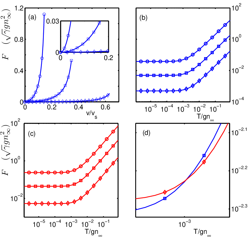
where all the derivatives are performed analytically using Eq. (8) and Eqs. (2–5) of [23]. The results are shown in Fig. 2(a) for the case of zero temperature. The fact that the force is nonzero below the critical velocity may be unexpected, although we note the magnitude is much smaller than the supercritical forces present above [14]. We emphasise that quasiparticle creation is not the mechanism behind this drag force, and consequentially this is not a contradiction of Landau’s statements [7]. At zero temperature fluctuations in the quantum vacuum scatter from each side of the impurity, and the asymmetric Doppler shift in the reflected waves results in an imbalance and a non-zero net force. A crucial assumption in this result is that the incoming waves have no knowledge of the impurity. In any finite system this assumption would only be valid up to a time after the initial acceleration of the impurity. It could be imagined that the force on the impurity will decay to zero over this time scale , which can be thought of as the relaxation time of the quantum vacuum. We intend to test this conjecture by performing dynamical simulations that incorporate the effects of the quantum fluctuations; this significant project lies beyond the scope of this work.
The results at finite temperature are shown in Fig. 2(b–d). The quantum and thermal regimes are clearly distinguished with a cross-over near . The force increases linearly with in the thermal regime due to the scattering being most prominent for the low energy modes whose occupation is for . The reflected modes for the high energy incoming waves have a negligible Doppler shift and only a small contribution to the force.
In conclusion, we have calculated the drag force acting on an impurity moving through a true BEC, in a quasi-1D geometry, using analytic solutions of the Bogoliubov perturbation expansion. We find that a nonzero force arises for zero and finite temperature at all velocities due to an imbalance in the Doppler shift in the scattering of quantum and thermal fluctuations. The crossover from the quantum to the thermal regime occurs at temperatures near . We have proposed a mechanism that predicts a time scale of for which it would be possible to observe the force in a finite system.
The authors wish to thank Tod Wright, Dmitry Petrov, Qian Niu, and Nicolas Pavloff for insightful discussions. AGS acknowledges the hospitality and support of the Center for Nonlinear Studies. AGS and MJD acknowledge support from the Australian Research Council Centre of Excellence for Quantum-Atom Optics.
References
- [1] A. Görlitz et al., Phys. Rev. Lett. 87, 130402 (2001); F. Schreck et al., ibid. 87, 080403 (2001); M. Greiner et al., ibid. 87, 160405 (2001); S. Richard et al., ibid. 91, 010405 (2003); H. Moritz et al., ibid. 91, 250402 (2003).
- [2] B. Laburthe Tolra et al., Phys. Rev. Lett. 92, 190401 (2004).
- [3] T. Kinoshita, T. Wenger, and D. S. Weiss, Science 305 1125 (2004); Phys. Rev. Lett. 95, 190406 (2005).
- [4] S. Hofferberth et al., Nature (London) 449, 324 (2007).
- [5] A. H. van Amerongen et al., Phys. Rev. Lett. 100, 090402 (2008).
- [6] C. Raman et al., Phys. Rev. Lett. 83, 2502 (1999); R. Onofrio et al., ibid. 85, 2228 (2000); D. E. Miller et al., ibid. 99, 070402 (2007); C. Ryu et al., ibid. 99, 260401 (2007); P. Engels, and C. Atherton, ibid. 99, 160405 (2007).
- [7] L. D. Landau, J. Phys. (Moscow) 5, 71 (1941); R. P. Feynman, in Progress in Low Temperature Physics, Vol. I, (North-Holland, Amsterdam, 1955).
- [8] D. C. Roberts and Y. Pomeau, Phys. Rev. Lett. 95, 145303 (2005); D. C. Roberts, Phys. Rev. A 74, 013613 (2006); D. C. Roberts Contemp. Phys. 50, 453-461 (2009).
- [9] Stefan Palzer, Cristoph Zipkes, Carlos Sias and Michael Köhl, arXiv:0903.4823.
- [10] M. Olshanii, Phys. Rev. Lett. 81, 938 (1998).
- [11] D. S. Petrov, G. V. Shlyapnikov and J. T. M. Walraven, Phys. Rev. Lett. 85, 3745 (2000).
- [12] C. Mora and Y. Castin, Phys. Rev. A 67, 053615 (2003); Yu. Kagan, B. V. Svistunov, and G. V. Shlyapnikov, Sov. Phys. JETP 66, 314 (1987).
- [13] G. E. Astrakharchik and L. P. Pitaevskii, Phys. Rev. A 70, 013608 (2004); H. P. Büchler, V. B. Geshkenbein, and G. Blatter, Phys. Rev. Lett. 87, 100403 (2001).
- [14] V. Hakim, Phys. Rev. E 55, 2835 (1997); Nicolas Pavloff, Phys. Rev. A 66, 013610 (2002).
- [15] T. Frisch, Y. Pomeau and S. Rica, Phys. Rev. Lett. 69, 1644 (1992); T. Winiecki, J. F. McCann and C. S. Adams, ibid. 82, 5186 (1999).
- [16] D. Taras-Semchuk and J. M. F. Gunn, Phys. Rev. B 60, 13139 (1999).
- [17] T. Tsuzuki, J. Low Temp. Phys. 4, 441 (1971).
- [18] Y. Castin and R. Dum, Phys. Rev. A 57 3008 (1998); S. A. Morgan, Phys. Rev. A 69, 023609 (2004).
- [19] X.-J. Chen, Z.-D. Chen, and N.-N. Huang, J. Phys. A 31, 6929 (1998).
- [20] N. Bilas and N. Pavloff, Phys. Rev. A 72, 033618 (2005).
- [21] A. L. Fetter, Annals of Physics 70, 67 (1972).
- [22] D. S. Petrov, D. M. Gangardt and G. V. Shlyapnikov, J. Phys. IV France 1 (2008).
- [23] EPAPS Document No. X-XXXXXX-XXX-XXXXXX
I AUXILLIARY PUBLICATION FOR: Drag force on an impurity below the superfluid critical velocity in a quasi-one-dimensional Bose-Einstein condensate
Here we describe the solution of Eq. (11) in the main text (repeated here for convenience)
| (14) |
where is the identity. We begin by writing down the four linear independent solutions to the homogenous equation
| (15) |
for the separate cases of and . These are denoted (recall that the ket notation refers to a complex conjugate pair) where,
| (16) | ||||
| (17) | ||||
| (18) | ||||
| (19) |
To the best of our knowledge, Eqs. (18) and (19) do not appear in the previous literature. Note from these solutions, the behaviour as : constant, 0, linear increase/decrease, and exponential increase/decrease, which can be seen from Fig. 3.
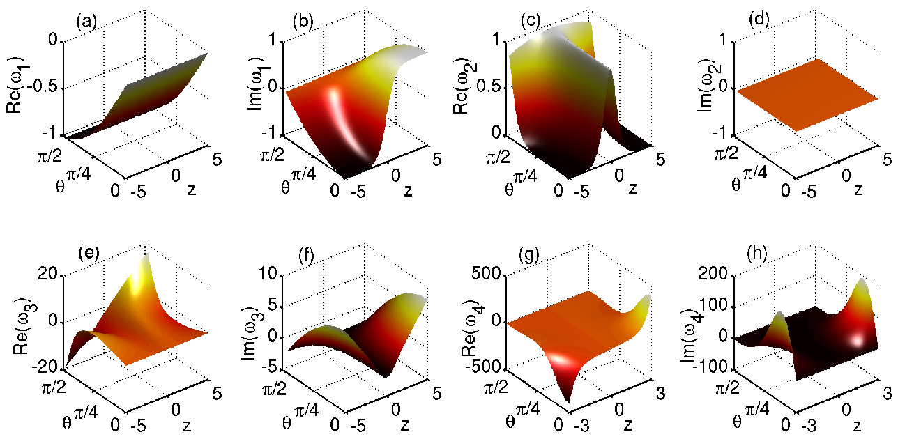
Using these eight functions (where always runs over the indices ) we construct four linearly independent solutions (denoted ) to Eq. (15) for the entire domain . This is done by matching the solutions in across the point subject to the conditions
| (20a) | ||||
| (20b) | ||||
which are the usual conditions appropriate for the term in the differential operator . The result is
where and are determined from Eqs. (20) above.
The next step involves finding which is a solution to Eq. (11) of the main article. We write
| (29) |
With some work it can be shown that the conditions
| (30a) | ||||
| (30b) | ||||
are completely equivalent to the following equations
| (31) | ||||
| (32) | ||||
| (33) | ||||
| (34) |
This is a satisfying result that can be anticipated from the fact that the operator is self-adjoint, and that vectors and should always be solutions to the adjoint problem.
To remove the components of which have an exponential divergence at , we impose the conditions
| (35) | ||||
| (36) |
Enforcing the symmetry of the Green’s matrix results in
| (37) | ||||
| (38) | ||||
| (39) | ||||
| (40) | ||||
| (41) |
where and .
The final condition to ensure the Green’s matrix is unique relates to how the system responds to the broken symmetry caused by the moving impurity. The force could be either positive or negative, and the physically correct solution is when the force is positive as this is the only energy conserving solution. This gives
| (42) | ||||
| (43) | ||||
| (44) |
and completes the solution to Eq. (11) of the main article.
