Evidences in favor of an accelerating cosmic expansion are now quite numerous, reaching from the first systematic observations of Type Ia supernovae [1] to the more recent WMAP survey of the Cosmic Microwave Background [2]. The standard interpretation of this acceleration, in the form of a cosmological constant [3], raises major well known questions. In particular it is not understood why the observed value of the vacuum energy density associated with the cosmological constant is so close to the non relativistic matter energy density (the so called coincidence problem) and so far from the “natural” order of magnitude expected from high energy physics [4].

The problem is that the geometry reconstructed from observation is not sourced by known matter according to the Einstein equation,

$$\Bigl(R_{\mu\nu}-\frac{1}{2}g_{\mu\nu}R\Bigr)_{\rm obs}\neq\Bigl(8\pi G_{N}T_{\mu\nu}\Bigr)_{\rm known}\;.$$

(1)

Different ways addressing this problem can be classified as to whether it is the right hand (matter) side or the left hand (gravity) side of (1) which is modified. “Dark energy” models explain the data by introducing a new source of stress energy to the right hand side of (1). A cosmological constant is one example; another is a scalar quintessence field $\varphi$ described by the Lagrangian [5],

$$\mathcal{L}=-\frac{1}{2}\partial_{\mu}\varphi\partial_{\nu}\varphi g^{\mu\nu}\sqrt{-g}-V(\varphi)\sqrt{-g}\;.$$

(2)

Local, metric-based modifications to the left hand side of (1) are restricted by stability [6] to take the form of replacing the Ricci scalar of the Hilbert Lagrangian by an arbitrary function of the Ricci scalar [7, 8],

$$-\frac{1}{16\pi G_{N}}\,R\sqrt{-g}\longrightarrow-\frac{1}{16\pi G_{N}}\,F(R)\sqrt{g}\;.$$

(3)

More general modifications of gravity must either abandon stability or locality [9, 10, 11, 12], or they must involve some field other than the metric to carry part of the gravitational force [13, 14]. Other proposals involving extra dimensions or massive gravitons have not yet reached a fully satisfactory state [15, 16].

Central to the evaluation of any class of models is the reconstruction problem. This consists of identifying the extent to which parameters in the model such as $V(\varphi)$ and $F(R)$ can be adjusted to support a geometry of the Friedmann-Lemaître-Robertson-Walker (FLRW) form with flat spatial sections,

$$ds^{2}=-dt^{2}+a^{2}(t)d\vec{x}\!\cdot\!d\vec{x}\;,$$

(4)

where the scale factor $a(t)$ is a known but arbitrary function of time. Of course there is just one expansion history in nature and a putative model need only explain that, but if reconstruction can be solved for a general scale factor then it is certain a model within the given class can fit the actual expansion history. To the extent that the solution is constructive one also obtains important constraints on the model, of course limited by the precision with which the expansion history can be measured.

It is straightforward to solve the reconstruction problem for scalar quintessence models [9, 17, 8] and a brief presentation of the solution will help focus ideas. For the FLRW geometry (4) the scalar must be independent of space, and only two of Einstein’s equations are nontrivial,

	$\displaystyle 3H^{2}$	$\displaystyle=$	$\displaystyle 8\pi G_{N}\Bigl[\frac{1}{2}\dot{\varphi}^{2}+V(\varphi)\Bigr]\;,$		(5)
	$\displaystyle-2\dot{H}-3H^{2}$	$\displaystyle=$	$\displaystyle 8\pi G_{N}\Bigl[\frac{1}{2}\dot{\varphi}^{2}-V(\varphi)\Bigr]\;.$		(6)

Here and henceforth, $G_{N}$ is the Newton constant, a dot means a derivative with respect to the cosmic time $t$ and we shall henceforth employ the usual definition of the Hubble parameter, $H\equiv\dot{a}/a$. By adding (5) and (6) one obtains the relation,

$$-2\dot{H}=8\pi G_{N}\,\dot{\varphi}^{2}\;.$$

Hence one can reconstruct the scalar’s evolution, and even invert it to express time in terms of the scalar, provided the Hubble parameter is monotonically decreasing,

$$\varphi(t)=\varphi_{0}\pm\int_{0}^{t}\!\!du\sqrt{\frac{-2\dot{H}(u)}{8\pi G_{N}}}\qquad\Longleftrightarrow\qquad t=t(\varphi)\;.$$

(7)

One then determines the potential by subtracting (6) from (5) and evaluating the resulting (assumed known) function of time at $t(\varphi)$,

$$\Bigl[2\dot{H}(t)+6H^{2}(t)\Bigr]_{t(\varphi)}=16\pi G_{N}\,V(\varphi)\;.$$

(8)

Similar reconstruction procedures exist for $F(R)$ models [6, 8]. The purpose of this paper is to solve the reconstruction problem for a recently proposed nonlocal cosmology model in which one multiplies the Hilbert Lagrangian by an algebraic function of the inverse scalar d’Alembertian acting on the Ricci scalar [12],

$${\cal L}_{g}\equiv\frac{1}{16\pi G_{N}}\,\sqrt{-g}R\left[1+f\Bigl(\frac{1}{\kern 1.0pt\vbox{\hrule height=1.2pt\hbox{\vrule width=1.2pt\hskip 3.0pt\vbox{\vskip 6.0pt}\hskip 3.0pt\vrule width=0.6pt}\hrule height=0.6pt}\kern 1.0pt}R\Bigr)\right]\;,$$

(9)

The motivation for this class of models is to trigger late time acceleration by the transition from radiation domination, during which the Ricci scalar is nearly zero, to matter domination at about $10^{5}$ years after the Big Bang. The subsequent time lag to the observed onset of acceleration, at about $10^{9}$ years, would be provided by the effect of the transition being reflected through the nonlocal, inverse d’Alembertian. Although there is hope of eventually deriving a model of the class (9) from quantum field theoretic loop corrections, the proposal is at this stage purely phenomenological.

The free parameter $f(X)$ in expression (9) is known as the nonlocal distortion function. Absent a derivation from fundamental theory, it has the same status as the potential $V(\varphi)$ in (2) and the function $F(R)$ in (3). What we will do in this paper is first to show how $f(X)$ can be tuned to give an arbitrary $a(t)$, then we will work out the specific form $f(X)$ must take to reproduce the $a(t)$ of $\Lambda$CDM, without actually employing a cosmological constant. This problem has already been studied in an excellent paper by Koivisto [18] (see also [19]) but for a local variant of the model, introduced by Nojiri and Odintsov [20], in which a scalar Lagrange multiplier forces the d’Alembertian of a second scalar give $R$. That version of the model has additional degrees of freedom that the original proposal lacks [21], so it is important to examine the reconstruction problem in both formulations.

This paper is organized as follows. In section 2 we summarize the model of Ref. [12] and its specialization to cosmology. In section 3 we outline the steps of the reconstruction of the function $f(X)$ once a given cosmology is chosen. In section 4, we show how to obtain the function $f$ suitable to reproduce the $\Lambda$CDM cosmological evolution with the same matter content but no cosmological constant. We then summarize our results and conclude in section 5.

The modified gravity Lagrangian (9) has already been given. It remains to state that             is the covariant scalar d’Alembertian,

$$\kern 1.0pt\vbox{\hrule height=1.2pt\hbox{\vrule width=1.2pt\hskip 3.0pt\vbox{\vskip 6.0pt}\hskip 3.0pt\vrule width=0.6pt}\hrule height=0.6pt}\kern 1.0pt\equiv\frac{1}{\sqrt{-g}}\,\partial_{\mu}\Bigl(\sqrt{-g}g^{\mu\nu}\partial_{\nu}\Bigr)\;.$$

By its inverse we mean the retarded Green’s function. For the FLRW geometry (4) the action of this inverse on some function of time $W(t)$ takes the simple form,

$$\frac{1}{\kern 1.0pt\vbox{\hrule height=1.2pt\hbox{\vrule width=1.2pt\hskip 3.0pt\vbox{\vskip 6.0pt}\hskip 3.0pt\vrule width=0.6pt}\hrule height=0.6pt}\kern 1.0pt}\Bigl[W\Bigr](t)=-\int_{0}^{t}\!\!du\,\frac{1}{a^{3}(u)}\int_{0}^{u}\!\!dv\,a^{3}(v)W(v)\;.$$

(10)

The metric $g_{\mu\nu}$ is assumed to be minimally coupled to matter.

The model is actually defined by its field equations, which are obtained by varying the gravity and matter actions with respect to the metric and then employing the partial integration trick explained in [11]. This produces causal and conserved field equations, like those of the more rigorous Schwinger-Keldysh formalism [22]. These equations take the form,

$\displaystyle G_{\mu\nu}+\Delta G_{\mu\nu}=8\pi G_{N}T_{\mu\nu},$

(11)

where $T_{\mu\nu}$ is the matter total energy momentum tensor (including a possibly non vanishing cosmological constant), and $\Delta G_{\mu\nu}$ comes from varying the non local $f$ term in the above action (9).

In the following, we will restrict the metric to be of FLRW form (4). With this ansatz, the field equations (11) take the form

	$\displaystyle 3H^{2}+\Delta G_{00}$	$\displaystyle=$	$\displaystyle 8\pi G\rho,$		(12)
	$\displaystyle-2\dot{H}-3H^{2}+\frac{1}{3a^{2}}\delta^{ij}\Delta G_{ij}$	$\displaystyle=$	$\displaystyle 8\pi GP,$		(13)

$\rho$ and $P$ being respectively the matter total energy density and pressure, and the non local pieces reading

	$\displaystyle\Delta G_{00}=\Bigl[3H^{2}+3H\partial_{t}\Bigr]\Biggl\{f\Bigl(\frac{1}{\kern 1.0pt\vbox{\hrule height=1.2pt\hbox{\vrule width=1.2pt\hskip 3.0pt\vbox{\vskip 6.0pt}\hskip 3.0pt\vrule width=0.6pt}\hrule height=0.6pt}\kern 1.0pt}R\Bigr)+\frac{1}{\kern 1.0pt\vbox{\hrule height=1.2pt\hbox{\vrule width=1.2pt\hskip 3.0pt\vbox{\vskip 6.0pt}\hskip 3.0pt\vrule width=0.6pt}\hrule height=0.6pt}\kern 1.0pt}\Biggl[Rf^{\prime}\Bigl(\frac{1}{\kern 1.0pt\vbox{\hrule height=1.2pt\hbox{\vrule width=1.2pt\hskip 3.0pt\vbox{\vskip 6.0pt}\hskip 3.0pt\vrule width=0.6pt}\hrule height=0.6pt}\kern 1.0pt}R\Bigr)\Biggr]\Bigg\}$				(14)
			$\displaystyle\hskip 142.26378pt+\frac{1}{2}\partial_{t}\Bigl(\frac{1}{\kern 1.0pt\vbox{\hrule height=1.2pt\hbox{\vrule width=1.2pt\hskip 3.0pt\vbox{\vskip 6.0pt}\hskip 3.0pt\vrule width=0.6pt}\hrule height=0.6pt}\kern 1.0pt}R\Bigr)\times\partial_{t}\Biggl(\frac{1}{\kern 1.0pt\vbox{\hrule height=1.2pt\hbox{\vrule width=1.2pt\hskip 3.0pt\vbox{\vskip 6.0pt}\hskip 3.0pt\vrule width=0.6pt}\hrule height=0.6pt}\kern 1.0pt}\Biggl[Rf^{\prime}\Bigl(\frac{1}{\kern 1.0pt\vbox{\hrule height=1.2pt\hbox{\vrule width=1.2pt\hskip 3.0pt\vbox{\vskip 6.0pt}\hskip 3.0pt\vrule width=0.6pt}\hrule height=0.6pt}\kern 1.0pt}R\Bigr)\Biggr]\Biggr),\qquad$
	$\displaystyle\Delta G_{ij}=-\Bigl[2\dot{H}+3H^{2}+2H\partial_{t}+\partial_{t}^{2}\Bigr]\Biggl\{f\Bigl(\frac{1}{\kern 1.0pt\vbox{\hrule height=1.2pt\hbox{\vrule width=1.2pt\hskip 3.0pt\vbox{\vskip 6.0pt}\hskip 3.0pt\vrule width=0.6pt}\hrule height=0.6pt}\kern 1.0pt}R\Bigr)+\frac{1}{\kern 1.0pt\vbox{\hrule height=1.2pt\hbox{\vrule width=1.2pt\hskip 3.0pt\vbox{\vskip 6.0pt}\hskip 3.0pt\vrule width=0.6pt}\hrule height=0.6pt}\kern 1.0pt}\Biggl[Rf^{\prime}\Bigl(\frac{1}{\kern 1.0pt\vbox{\hrule height=1.2pt\hbox{\vrule width=1.2pt\hskip 3.0pt\vbox{\vskip 6.0pt}\hskip 3.0pt\vrule width=0.6pt}\hrule height=0.6pt}\kern 1.0pt}R\Bigr)\Biggr]\Bigg\}g_{ij}$				(15)
			$\displaystyle\hskip 142.26378pt+\frac{1}{2}\partial_{t}\Bigl(\frac{1}{\kern 1.0pt\vbox{\hrule height=1.2pt\hbox{\vrule width=1.2pt\hskip 3.0pt\vbox{\vskip 6.0pt}\hskip 3.0pt\vrule width=0.6pt}\hrule height=0.6pt}\kern 1.0pt}R\Bigr)\times\partial_{t}\Biggl(\frac{1}{\kern 1.0pt\vbox{\hrule height=1.2pt\hbox{\vrule width=1.2pt\hskip 3.0pt\vbox{\vskip 6.0pt}\hskip 3.0pt\vrule width=0.6pt}\hrule height=0.6pt}\kern 1.0pt}\Biggl[Rf^{\prime}\Bigl(\frac{1}{\kern 1.0pt\vbox{\hrule height=1.2pt\hbox{\vrule width=1.2pt\hskip 3.0pt\vbox{\vskip 6.0pt}\hskip 3.0pt\vrule width=0.6pt}\hrule height=0.6pt}\kern 1.0pt}R\Bigr)\Biggr]\Biggr)g_{ij}\;,\qquad$

where $f^{\prime}$ denotes the derivative of $f$ with respect to its argument. As already stressed, the left hand side of equation (11) is conserved, and hence the first Friedmann equation (12) and the matter energy-momentum conservation equation,

$\displaystyle\dot{\rho}+3H(P+\rho)=0,$

(16)

are enough to ensure that equation (13) is fulfilled, as is the case with standard Friedmann equations.

We first note that the difference between field equations (12) and (13) leads to a simple second order ODE for the function $F$ defined as

$\displaystyle F$

$\displaystyle=$

$\displaystyle f+\frac{1}{\kern 1.0pt\vbox{\hrule height=1.2pt\hbox{\vrule width=1.2pt\hskip 3.0pt\vbox{\vskip 6.0pt}\hskip 3.0pt\vrule width=0.6pt}\hrule height=0.6pt}\kern 1.0pt}\left(R\frac{df}{dX}\right),$

(17)

where $X$ is defined as

$\displaystyle X\equiv\frac{1}{\kern 1.0pt\vbox{\hrule height=1.2pt\hbox{\vrule width=1.2pt\hskip 3.0pt\vbox{\vskip 6.0pt}\hskip 3.0pt\vrule width=0.6pt}\hrule height=0.6pt}\kern 1.0pt}{R}.$

(18)

This ODE reads

$\displaystyle\ddot{F}+5H\dot{F}+\left(6H^{2}+2\dot{H}\right)\left(F+1\right)=8\pi G_{N}\left(\rho-P\right).$

(19)

If one then assumes the matter content of the Universe (specified here-above by its total energy density $\rho$ and pressure $P$) and its cosmological evolution (specified by some scale factor $a(t)$) to be chosen, the first step to reconstruct $f$ is to solve Eq. (19), which allows to obtain $F$ as a function of the cosmological time $t$. Then we invert relation (17) rewritten as

$\displaystyle\kern 1.0pt\vbox{\hrule height=1.2pt\hbox{\vrule width=1.2pt\hskip 3.0pt\vbox{\vskip 6.0pt}\hskip 3.0pt\vrule width=0.6pt}\hrule height=0.6pt}\kern 1.0ptF=\kern 1.0pt\vbox{\hrule height=1.2pt\hbox{\vrule width=1.2pt\hskip 3.0pt\vbox{\vskip 6.0pt}\hskip 3.0pt\vrule width=0.6pt}\hrule height=0.6pt}\kern 1.0ptf+R\dot{f}\frac{dX}{dt},$

(20)

and yielding thus an ODE provided $X$ is known as a function of $t$ via equation (18). This allows to obtain $f$ as a function¹¹ 1 Denoting here by the same letter the function $f(t)\equiv f(X(t))$ and the function $f(X)$ of $t$. The last step is to invert $X(t)$ to obtain $t$ as a function of $X$. This allows to get $f(X)$, the function which appears in the original action (9).

In this process, some care has to be taken about the boundary conditions. First, we emphasize that our choice of the retarded Green function in the definition of the inverse of the d’Alembertian operator (10) does not permit inclusion of the extra zero modes that cause the ambiguities underlined in Ref. [21] about the local version of the model considered in [18, 20]. Moreover, one should make sure that whatever boundary conditions get imposed to integrate the ODEs are compatible with both equations (12) and (13). The need for this might seem confusing in view of the close relation between the two equations implied by conservation,

$$\Bigl[\frac{d}{dt}+3H\Bigr]\Bigl({\rm Eqn.}~\ref{EQrho}\Bigr)=-3H\times\Bigl({\rm Eqn.}~\ref{EQP}\Bigr)\;.$$

(21)

However, it will be noted that relation (21) involves a derivative of equation (12). Had we based the reconstruction technique solely upon equation (12) then equation (13) would have followed automatically. But our reconstruction procedure instead employs the difference of equations (12) and (13), and this difference only defines equation (12) up to an integration constant.

In the next section, we carry out these steps for the special case where the matter content of the Universe only consists of non relativistic and relativistic matter without any cosmological constant, while the cosmological evolution is that given by usual Friedmann equation with the same matter content plus a non vanishing cosmological constant, i.e. the one of the $\Lambda$CDM model.

We want to reproduce $\Lambda$CDM cosmology with the same matter content but a vanishing cosmological constant. Hence we assume that the Hubble parameter $H$, appearing in equation (19), is a solution of the standard Friedmann equations with a cosmological constant and the same matter content as in our Universe:

	$\displaystyle 3H^{2}-\Lambda$	$\displaystyle=$	$\displaystyle 8\pi G\rho,$		(22)
	$\displaystyle 2\dot{H}+3H^{2}-\Lambda$	$\displaystyle=$	$\displaystyle-8\pi GP.$		(23)

It is then easy to see that Eq (19) simplifies dramatically to read now

$$\ddot{F}+5H\dot{F}+\left(6H^{2}+2\dot{H}\right)F=-6H_{0}^{2}\Omega_{\Lambda},$$

(24)

where $H_{0}$ is the Hubble parameter today, and $\Omega_{\Lambda}$ is defined as usual in terms of the cosmological constant $\Lambda$ entering into equations (22-23), i.e. as

$\displaystyle\Omega_{\Lambda}=\frac{\Lambda}{3H_{0}^{2}}.$

(25)

Notice that the matter energy density and pressure appearing on the right hand side of equation (19) have cancelled against $6H^{2}+2\dot{H}$ appearing on the left hand side.

In the rest of the paper, we will further simplify the problem by considering that the only matter content of the Universe is a sum of two components, one of non relativistic matter (with $\Omega$ parameter $\Omega_{m}$) and one of relativistic matter (with $\Omega$ parameter $\Omega_{r}$). It will then turn out to be convenient to use equations (22) and (23) to reexpress $H$ and its time derivatives in terms of $\Omega_{\Lambda}$, $\Omega_{r}$ and $\Omega_{m}$ and to use the variable $\zeta$ instead of $t$, defined in terms of the redshift $z$ as

$$\zeta\equiv 1+z=\frac{1}{a(t)}.$$

We also introduce the dimensionless Hubble parameter $h(\zeta)$ given by

$\displaystyle h(\zeta)=\sqrt{\Omega_{\Lambda}+\Omega_{m}\zeta^{3}+\Omega_{r}\zeta^{4}},=H/H_{0}.$

(26)

Equation (24) can be readily integrated²² 2 Using that the fact that $\zeta^{2}$ is a homogeneous solution. to yield $F$ in the form

$\displaystyle F\equiv\zeta^{2}\Phi^{2},$

(27)

where $\Phi$ is given by

$\displaystyle\Phi(\zeta)$

$\displaystyle=$

$\displaystyle\Phi_{\rm eq}+h(\zeta_{\rm eq})\Phi^{\prime}_{\rm eq}\int_{\zeta_{\rm eq}}^{\zeta}\frac{d\zeta_{1}}{h(\zeta_{1})}-6\Omega_{\Lambda}\int_{\zeta_{\rm eq}}^{\zeta}\frac{d\zeta_{1}}{h(\zeta_{1})}\int_{\zeta_{\rm eq}}^{\zeta_{1}}\frac{d\zeta_{2}}{\zeta_{2}^{4}h(\zeta_{2})},$

and the integration constants $\Phi_{\rm eq}$ and $\Phi^{\prime}_{\rm eq}$ are defined respectively as the values of $\Phi$ and $\Phi^{\prime}$ (here and in the following, a prime denotes a derivative with respect to $\zeta$) at the matter-radiation equality $\zeta_{\rm eq}$. In order to have a well behaved $F$ at early times, we demand that $F(\zeta)$ goes to zero at large $\zeta$. This fixes $\Phi_{\rm eq}$ and $\Phi^{\prime}_{\rm eq}$ to be

	$\displaystyle\Phi_{\rm eq}$	$\displaystyle=$	$\displaystyle-6\Omega_{\Lambda}\int_{\zeta_{\rm eq}}^{\infty}\!\!d\zeta_{1}\,\frac{1}{h(\zeta_{1})}\int_{\zeta_{1}}^{\infty}\!\!d\zeta_{2}\,\frac{1}{\zeta_{2}^{4}h(\zeta_{2})}\;.$		(28)
	$\displaystyle\Phi_{\rm eq}^{\prime}$	$\displaystyle=$	$\displaystyle\frac{6\Omega_{\Lambda}}{h_{\rm eq}}\int_{\zeta_{\rm eq}}^{\infty}\!\!d\zeta_{1}\,\frac{1}{\zeta_{1}^{4}h(\zeta_{1})}.$		(29)

The resulting expression for $\Phi(\zeta)$ is then given by

$$\Phi(\zeta)=-6\Omega_{\Lambda}\int_{\zeta}^{\infty}\!\!d\zeta_{1}\,\frac{1}{h(\zeta_{1})}\int_{\zeta_{1}}^{\infty}\!\!d\zeta_{2}\,\frac{1}{\zeta_{2}^{4}h(\zeta_{2})}\;,$$

and the large $\zeta$ expansion of $\Phi(\zeta)$ is,

$$\Phi(\zeta)=-\frac{\Omega_{\Lambda}}{5\Omega_{r}}\,\frac{1}{\zeta^{6}}+{\cal O}\Bigl(\frac{1}{\zeta^{7}}\Bigr)\;.$$

Any choice other than (28-29) will result in a function $F(\zeta)$ actually growing for large $\zeta$.

Having obtained $F(\zeta)$ we now turn to invert equation (17). This equation reads,

$\displaystyle\frac{\zeta^{2}h^{2}}{(2\Omega_{\Lambda}+\frac{1}{2}\Omega_{m}\zeta^{3})}\frac{d^{2}}{d\zeta^{2}}\left(f-F\right)-\frac{df}{d\zeta}\left(\zeta+6\frac{d\zeta}{dX}\right)=-\zeta\frac{dF}{d\zeta}.$

(30)

Knowing $F$ from (27) it can easily be integrated once to yield the general solution

	$\displaystyle\frac{df}{d\zeta}=2\zeta\Phi(\zeta)+\frac{\zeta^{2}}{h(\zeta)I(\zeta)}\Biggl\{\Bigl[(f^{\prime})_{eq}\!-\!2\Phi_{eq}\Bigr]\frac{h_{eq}I_{eq}}{\zeta_{eq}^{2}}$				(31)
			$\displaystyle\hskip 42.67912pt+6\Omega_{\Lambda}\int_{\zeta}^{\zeta_{eq}}\!\!d\zeta_{1}\,\frac{I(\zeta_{1})}{\zeta_{1}^{4}h(\zeta_{1})}-2\int_{\zeta}^{\zeta_{eq}}\!\!d\zeta_{1}\,\frac{(12\Omega_{\Lambda}\!+\!3\Omega_{m}\zeta_{1}^{3})\Phi(\zeta_{1})}{\zeta_{1}^{5}}\Biggr\}\;.\qquad$

This expression contains a new integration constant, $(f^{\prime})_{eq}$, and the function $I(\zeta)$ defined by

$\displaystyle I(\zeta)\equiv\int^{\infty}_{\zeta}\frac{d\zeta_{1}}{\zeta_{1}^{4}H_{0}H(\zeta_{1})}R,=\int_{\zeta}^{\infty}\!\!d\zeta_{1}\,\frac{(12\Omega_{\Lambda}\!+\!3\Omega_{m}\zeta_{1}^{3})}{\zeta_{1}^{4}h(\zeta_{1})}\;.$

(32)

Now, one also has from equation (17) that

	$\displaystyle F(\zeta)$	$\displaystyle=$	$\displaystyle f\Bigl(X(\zeta)\Bigr)-\int_{\zeta}^{\infty}\!\!d\zeta_{1}\,\frac{\zeta_{1}^{2}}{h(\zeta_{1})}\int_{\zeta_{1}}^{\infty}\!\!d\zeta_{2}\,\frac{(12\Omega_{\Lambda}\!+\!3\Omega_{m}\zeta_{2}^{3})}{\zeta_{2}^{4}h(\zeta_{2})}\times\frac{df}{dX}\;,\qquad$		(33)
		$\displaystyle=$	$\displaystyle f\Bigl(X(\zeta)\Bigr)-\int_{\zeta}^{\infty}\!\!d\zeta_{1}\,\frac{\zeta_{1}^{2}}{h(\zeta_{1})}\int_{\zeta_{1}}^{\infty}\!\!d\zeta_{2}\,\frac{(12\Omega_{\Lambda}\!+\!3\Omega_{m}\zeta_{2}^{3})}{\zeta_{2}^{6}I(\zeta_{2})}\times\frac{df}{d\zeta_{2}}\;.\qquad$

where we have used the the definition of $\kern 1.0pt\vbox{\hrule height=1.2pt\hbox{\vrule width=1.2pt\hskip 3.0pt\vbox{\vskip 6.0pt}\hskip 3.0pt\vrule width=0.6pt}\hrule height=0.6pt}\kern 1.0pt^{-1}$ given in equation (10). In particular, we have that

$$\frac{1}{\kern 1.0pt\vbox{\hrule height=1.2pt\hbox{\vrule width=1.2pt\hskip 3.0pt\vbox{\vskip 6.0pt}\hskip 3.0pt\vrule width=0.6pt}\hrule height=0.6pt}\kern 1.0pt}\Bigl[R\Bigr]=-\int_{\zeta}^{\infty}\!\!d\zeta_{1}\,\frac{\zeta_{1}^{2}}{h(\zeta_{1})}\int_{\zeta_{1}}^{\infty}\!\!d\zeta_{2}\,\frac{(12\Omega_{\Lambda}\!+\!3\Omega_{m}\zeta_{2}^{3})}{\zeta_{2}^{4}h(\zeta_{2})}\;=X(\zeta).$$

which was used to obtain equation (33). The integral in Eq. (33) will only make sense provided $df/d\zeta$ falls off faster that $1/\zeta^{2}$ for large $\zeta$. This fixes the new integration constant $(f^{\prime})_{\rm eq}$ to be

	$\displaystyle(f^{\prime})_{eq}=2\Phi_{eq}$				(34)
			$\displaystyle\hskip 22.76228pt+\frac{\zeta_{eq}^{2}}{h_{eq}I_{eq}}\Biggl\{6\Omega_{\Lambda}\!\!\int_{\zeta_{eq}}^{\infty}\!\!d\zeta_{1}\,\frac{I\zeta_{1})}{\zeta_{1}^{4}h(\zeta_{1})}-2\!\!\int_{\zeta_{eq}}^{\infty}\!\!d\zeta_{1}\,\frac{(12\Omega_{\Lambda}\!+\!3\Omega_{m}\zeta_{1}^{3})\Phi(\zeta_{1})}{\zeta_{1}^{5}}\Biggr\}\;,\qquad$

and results in the new expression for $df/d\zeta$ reading

	$\displaystyle\frac{df}{d\zeta}=2\zeta\Phi(\zeta)+\frac{\zeta^{2}}{h(\zeta)I(\zeta)}\Biggl\{6\Omega_{\Lambda}\int_{\zeta}^{\infty}\!\!d\zeta_{1}\,\frac{I(\zeta_{1})}{\zeta_{1}^{4}h(\zeta_{1})}$				(35)
			$\displaystyle\hskip 156.49014pt-2\int_{\zeta}^{\infty}\!\!d\zeta_{1}\,\frac{(12\Omega_{\Lambda}\!+\!3\Omega_{m}\zeta_{1}^{3})\Phi(\zeta_{1})}{\zeta_{1}^{5}}\Biggr\}\;.\qquad$

If one integrates once more, one obtains another integration constant, namely the value of $f(\zeta)$ at $\zeta=\zeta_{\rm eq}$. This constant can be fixed demanding that relation (33) hold at $\zeta=\zeta_{eq}$. We get

$$(f)_{eq}=\zeta_{eq}^{2}\Phi_{eq}-\int_{\zeta_{eq}}^{\infty}\!\!d\zeta_{1}\,\frac{\zeta_{1}^{2}}{h(\zeta_{1})}\int_{\zeta_{1}}^{\infty}\!\!d\zeta_{2}\,\frac{(12\Omega_{\Lambda}\!+\!3\Omega_{m}\zeta_{2}^{3})}{\zeta_{2}^{6}I(\zeta_{2})}\times\frac{df}{d\zeta_{2}}\;.$$

Note that this relation is not self-referential for $(f)_{eq}$ because the factor of $df/d\zeta^{\prime\prime}$ on the right hand side does not involve $(f)_{eq}$. With such a choice for $(f)_{eq}$, the function $f\Bigl(X(\zeta)\Bigr)$ vanishes at early times, that is, for large $\zeta$. We can therefore construct $f$ by simply integrating equation (35) to obtain

	$\displaystyle f\Bigl(X(\zeta)\Bigr)=-\int_{\zeta}^{\infty}\!\!d\zeta_{1}\,\frac{df}{d\zeta_{1}}\;,$				(36)
			$\displaystyle=-2\int_{\zeta}^{\infty}\!\!d\zeta_{1}\,\zeta_{1}\Phi(\zeta_{1})-6\Omega_{\Lambda}\int_{\zeta}^{\infty}\!\!d\zeta_{1}\,\frac{\zeta_{1}^{2}}{h(\zeta_{1})I(\zeta_{1})}\int_{\zeta_{1}}^{\infty}\!\!d\zeta_{2}\,\frac{I(\zeta_{2})}{\zeta_{2}^{4}h(\zeta_{2})}\qquad$
			$\displaystyle\hskip 28.45274pt+2\int_{\zeta}^{\infty}\!\!d\zeta_{1}\,\frac{\zeta_{1}^{2}}{h(\zeta_{1})I(\zeta_{1})}\int_{\zeta_{1}}^{\infty}\!\!d\zeta_{2}\,\frac{(12\Omega_{\Lambda}\!+\!3\Omega_{m}\zeta_{2}^{3})\Phi(\zeta_{2})}{\zeta_{2}^{5}}\;,\qquad$
			$\displaystyle=6\Omega_{\Lambda}\int_{\zeta}^{\infty}\!\!d\zeta_{1}\,\frac{(\zeta_{1}^{2}\!-\!\zeta^{2})}{h(\zeta_{1})}\int_{\zeta_{1}}^{\infty}\!\!d\zeta_{2}\,\frac{1}{\zeta_{2}^{4}h(\zeta_{1})}$
			$\displaystyle\hskip 28.45274pt-6\Omega_{\Lambda}\int_{\zeta}^{\infty}\!\!d\zeta_{1}\,\frac{\zeta_{1}^{2}}{h(\zeta_{1})I(\zeta_{1})}\int_{\zeta_{1}}^{\infty}\!\!d\zeta_{2}\,\frac{I(\zeta_{2})}{\zeta_{2}^{4}h(\zeta_{2})}$
			$\displaystyle\hskip 56.9055pt-36\Omega_{\Lambda}\int_{\zeta}^{\infty}\!\!d\zeta_{1}\,\frac{\zeta_{1}^{2}}{h(\zeta_{1})I(\zeta_{1})}\int_{\zeta_{1}}^{\infty}\!\!d\zeta_{2}\,\Biggl[\frac{(\Omega_{\Lambda}\!+\!\Omega_{m}\zeta_{1}^{3})}{\zeta_{1}^{4}}$
			$\displaystyle\hskip 128.0374pt-\frac{(\Omega_{\Lambda}\!+\!\Omega_{m}\zeta_{2}^{3})}{\zeta_{2}^{4}}\Biggr]\frac{1}{h(\zeta_{2})}\int_{\zeta_{2}}^{\infty}\!\!d\zeta_{3}\,\frac{1}{\zeta_{3}^{4}h(\zeta_{3})}\;.\qquad$

Introducing the variable $\alpha=\zeta_{eq}/\zeta$, as well as the parameter $\omega$ given by $\omega\equiv\Omega_{\Lambda}\Omega_{r}^{3}/\Omega_{m}^{4}$, the above expression for $f$ can be given in term of the two elliptic integrals $\overline{J}(\alpha)$ and $\overline{I}(\alpha)$ defined by

	$\displaystyle\overline{J}(\alpha)$	$\displaystyle\equiv$	$\displaystyle\int_{0}^{\alpha}\!\!d\alpha_{1}\,\frac{\alpha_{1}^{4}}{\sqrt{1\!+\!\alpha_{1}\!+\!\omega\alpha_{1}^{4}}}\;,$		(37)
	$\displaystyle\overline{I}(\alpha)$	$\displaystyle\equiv$	$\displaystyle\int_{0}^{\alpha}\!\!d\alpha_{1}\,\frac{\alpha_{1}\!+\!4\omega\alpha_{1}^{4}}{\sqrt{1\!+\!\alpha_{1}\!+\!\omega\alpha_{1}^{4}}}=\frac{\zeta_{eq}^{3/2}}{3\Omega_{m}^{1/2}}I(\zeta).$		(38)

If we then define $f_{1}$, $f_{2}$ and $f_{3}$ as the three contribution to $f$ appearing in the right hand side of equation (36), such that $f(\zeta)=f_{1}(\zeta)+f_{2}(\zeta)+f_{3}(\zeta)$, one has

	$\displaystyle f_{1}\Bigl(X(\zeta)\Bigr)$	$\displaystyle=$	$\displaystyle 6\omega\int_{0}^{\alpha}\!\!d\alpha_{1}\,\frac{(\frac{1}{\alpha_{1}^{2}}\!-\!\frac{1}{\alpha^{2}})\overline{J}(\alpha_{1})}{\sqrt{1\!+\!\alpha\!+\!\omega\alpha^{4}}}\;,$		(39)
	$\displaystyle f_{2}\Bigl(X(\zeta)\Bigr)$	$\displaystyle\!=\!$	$\displaystyle-6\omega\int_{0}^{\alpha}\!\!\!d\alpha_{1}\,\frac{1}{\alpha_{1}^{2}\sqrt{1\!+\!\alpha_{1}\!+\!\omega\alpha_{1}^{4}}\,\overline{I}(\alpha_{1})}\int_{0}^{\alpha_{1}}\!\!\!d\alpha_{2}\,\frac{\alpha_{2}^{4}\,\overline{I}(\alpha_{2})}{\sqrt{1\!+\!\alpha_{2}\!+\!\omega\alpha_{2}^{4}}}\;,\qquad$		(40)
	$\displaystyle f_{3}\Bigl(X(\zeta)\Bigr)$	$\displaystyle=$	$\displaystyle-12\omega\int_{0}^{\alpha}\!\!d\alpha_{1}\,\frac{1}{\alpha_{1}^{2}\sqrt{1\!+\!\alpha_{1}\!+\!\omega\alpha_{1}^{4}}\,\overline{I}(\alpha_{1})}$		(41)
			$\displaystyle\hskip 56.9055pt\times\int_{0}^{\alpha_{1}}\!\!d\alpha_{2}\,\frac{(\alpha_{1}\!+\!\omega\alpha_{1}^{4}\!-\!\alpha_{2}\!-\!\omega\alpha_{2}^{4})\,\overline{J}(\alpha_{2})}{\sqrt{1\!+\!\alpha_{2}\!+\!\omega\alpha_{2}^{4}}}\;,\qquad$		(42)

and one can use these expressions to numerically evolve $f\left(X(\zeta)\right)$.

Having thus obtained $f\left(X(\zeta)\right)$ as a function of $\zeta$, the last step is to get $\zeta$ as function of $X$. Before doing so, it is also of interest to check that nothing goes wrong at late times. For that purpose we need the following small $\zeta$ expansions,

	$\displaystyle h(\zeta)$	$\displaystyle=$	$\displaystyle\sqrt{\Omega_{\Lambda}}+\frac{\Omega_{m}}{2\sqrt{\Omega_{\Lambda}}}\,\zeta^{3}+O(\zeta^{4})\;,$		(43)
	$\displaystyle I(\zeta)$	$\displaystyle=$	$\displaystyle\frac{4\sqrt{\Omega_{\Lambda}}}{\zeta^{3}}-\frac{3\Omega_{m}}{\sqrt{\Omega_{\Lambda}}}\,\ln(\zeta)+O(1)\;,$		(44)
	$\displaystyle\Phi(\zeta)$	$\displaystyle=$	$\displaystyle-\frac{1}{\zeta^{2}}+O(1)\;.$		(45)

Now substitute these into each of the three terms in expression (35) for $df/d\zeta$ to get

$\displaystyle\frac{df}{d\zeta}=-\frac{2}{\zeta}+O(\zeta)+\Biggl[\frac{\zeta^{5}}{4\Omega}+O\Bigl(\zeta^{8}\ln(\zeta)\Bigr)\Biggr]\Biggl\{\frac{8\Omega_{\Lambda}}{\zeta^{6}}+O\Bigl(\frac{\ln(\zeta)}{\zeta^{3}}\Bigr)\Biggr\}=O(\zeta)\;.$

(46)

This implies that $f$ approaches a constant at late times. In the above equation (36), the three contributions appearing in the right hand side can be expressed using elliptic integrals.

Let us now turn to obtaining an expression for $X(\zeta)$. This also involves an elliptic integral. Indeed, equation (18) reads

$\displaystyle X=-\int^{\infty}_{\zeta}\frac{d\zeta_{1}\zeta_{1}^{2}}{H(\zeta_{1})}\int^{\infty}_{\zeta_{1}}\frac{d\zeta_{2}}{\zeta_{2}^{4}H(\zeta_{2})}R(\zeta_{2})\equiv-\int^{\infty}_{\zeta}\frac{d\zeta_{1}\zeta_{1}^{2}}{h(\zeta_{1})}I\left(\zeta_{1}\right),$

(47)

where $I$ is defined as in equation (32). For a chosen set of parameters $\{\Omega_{\Lambda},\Omega_{m},\Omega_{r}\}$, numerical evaluations of the right hand sides of equation (47) and (36) can easily be obtained, from which one can get $f$ as a function of $X$. The result is plotted in figure 1 for $\{\Omega_{\Lambda},\Omega_{m},\Omega_{r}\}$ = $\{0.72,0.28,8.5\times 10^{-5}\}$ which correspond to the latest WMAP values [2].

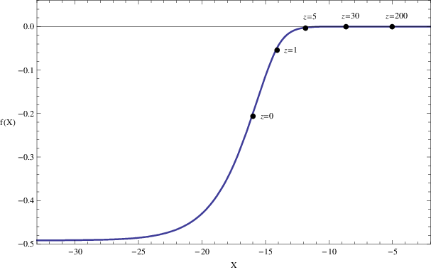
A simple analytic parameterization $f_{\rm an}$ of the found function $f$ is given by

$\displaystyle f_{\rm an}(X)=0.245\left[\tanh(0.350Y+0.032Y^{2}+0.003Y^{3})-1\right],$

(48)

where $Y$ is defined by $Y\equiv(X+16.5)$. It would hardly be distinguishable from the numerical solution should it be plotted together with the latter on figure 1. These numerical and analytic expressions for $f(X)$ allow us to resolve one of the major open questions about this class of models: do they make significant corrections to general relativity when expanded around flat space? The answer is “no.” One can see from Figure 1 that the curve is almost flat near $X=0$. From the analytic expression (48) we compute,

	$\displaystyle f_{\rm an}^{\prime}(0)$	$\displaystyle=$	$\displaystyle.245\Bigl[0.350+0.064Y_{0}+0.009Y_{0}^{2}\Bigr]$		(49)
			$\displaystyle\hskip 85.35826pt\times{\rm sech}^{2}\Bigl[0.350Y_{0}+0.032Y_{0}^{2}+0.003Y_{0}^{3}\Bigr]\;,$
		$\displaystyle\sim$	$\displaystyle 10^{-24}\;,$		(50)

where $Y_{0}=16.5$. So we find an utterly negligible linear correction.

In this work we have presented a general method to reproduce a given arbitrary cosmological evolution from a distorted non local form of the action for gravity as presented in Ref. [12]. This method was applied here to $\Lambda$CDM cosmology and we obtained the distortion function $f$ that leads, via action (9), to exactly the same cosmological evolution as in $\Lambda$CDM, with the same matter content but no cosmological constant. It is very interesting to note that the function we obtain numerically is almost indistinguishable from a simple analytic form (48). To be sure, this function contains some free parameters — for example, the value $X=-16.5$ where the $\tanh$ passes through zero, or the scaling of its full variation by $0.49$. However, these are all dimensionless numbers of order one. This is a consequence of two crucial properties of nonlocal models of type (3):

• •

  The onset of late time acceleration is triggered by the very recent cosmological transition from $R\approx 0$ during radiation domination to $R\sim 1/t^{2}$ during matter domination; and

• •

  Even after this transition the nonlocal operator $\frac{1}{\kern 1.0pt\vbox{\hrule height=1.2pt\hbox{\vrule width=1.2pt\hskip 3.0pt\vbox{\vskip 6.0pt}\hskip 3.0pt\vrule width=0.6pt}\hrule height=0.6pt}\kern 1.0pt}R\sim-\ln(t/t_{\rm eq})$ grows very slowly.

Several very interesting questions are left for future work. First, as far as cosmology is concerned, a natural question to address is if the model which gives the same background evolution as $\Lambda$CDM can be distinguished from $\Lambda$CDM by considering observables that contain information in addition to the background evolution. This requires in particular working out the theory of cosmological perturbations for the non local model (see [19]). To do so, a good starting point is in fact this work, using for example, the analytic form (when necessary) of the reconstructed distortion function. Other issues concern the various tests of gravity one can consider, in particular those in the solar system or those involving binary pulsars. It would be extremely interesting to apply those tests to the framework of Ref. [12], and a first investigation along these lines has already been carried out in Ref. [19]. Note in particular that the way cosmic acceleration is produced in the model considered here, is via a strengthening of the Newton constant encoded in the non local function $f$. However, the strengthening of the Newton constant we mentioned, strictly speaking only applies to cosmological distances, and things would be radically different, hence requiring a completely different analysis, inside gravitationally bound objects such as a galaxy or a cluster. This raises various questions about the effects of the non local operator $\kern 1.0pt\vbox{\hrule height=1.2pt\hbox{\vrule width=1.2pt\hskip 3.0pt\vbox{\vskip 6.0pt}\hskip 3.0pt\vrule width=0.6pt}\hrule height=0.6pt}\kern 1.0pt^{-1}$ inside matter.

RPW is grateful for the hospitality of the Laboratory APC, CNRS, University Paris 7, where a major part of this project was done. This work was partially supported by European Union grant INTERREG-IIIA, by NSF grant PHY-0653085, by the Institute for Fundamental Theory at the University of Florida, as well as the JCJC ANR grant ”MODGRAV”.

References

- [1] A. G. Riess et al., Astron. J. 116 (1998) 1009, astro-ph/9805201. S. Perlmutter et al., Astrophys. J. 517 (1999) 565, astro-ph/9812133.
- [2] J. Dunkley et al. [WMAP Collaboration], Astrophys. J. Suppl. 180 (2009) 306, arXiv:0803.0586 [astro-ph]. E. Komatsu et al. [WMAP Collaboration], Astrophys. J. Suppl. 180 (2009) 330, arXiv:0803.0547 [astro-ph].
- [3] Y. Wang and P. Mukherjee, Astrophys. J. 650 (2006) 1, astro-ph/0604051; U. Alam, V. Sahni and A. A. Starobinsky, JCAP 0702 011, 2007, astro-ph/0612381.
- [4] S. M Carroll, Living Rev. Rel. 4 (2001) 1, astro-ph/0004075.
- [5] C. Wetterich, Nucl. Phys. B302 (1988) 668; B. Ratra and P. J. E. Peebles, Phys. Rev. D37 (1988) 3406.
- [6] R. P. Woodard, Lect. Notes Phys. 720 (2007) 403, astro-ph/0601672.
- [7] S. Capozziello, S. Carloni and A. Troisi, Recent Res. Dev. Astron. Astrophys. 1 (2003) 625, astro-ph/0303041; S. M. Carroll, V. Duvvuri, M. Trodden and M. S. Turner, Phys. Rev. 70 (2004) 043528, astro-ph/0306438.
- [8] S. Capozziello, S. Nojiri and S. D. Odintsov, Phys. Lett. B634 (2006) 93, hep-th/0512118; S. Nojiri and S. D. Odintsov, Int. J. Geom. Meth. Phys. 4 (2007) 115, hep-th/0601213; Phys. Rev. D77 (2008) 026007, arXiv:0710.1738.
- [9] N. C. Tsamis and R. P. Woodard, Ann. Phys. 267 (1998) 145, hep-ph/9712331.
- [10] T. Banks, Nucl. Phys. B309 (1988) 493; D. Espriu, T. Multamaki and E. C. Vagenas, Phys. Lett. B628 (2005) 197, gr-qc/0503033; H. W. Hamber and R. M. Williams, Phys. Rev. D72 (2005), 044026, hep-th/0507017; T. Biswas, A. Mazumdar and W. Siegel, JCAP 0603 (2006) 009, hep-th/0508194; J. Khoury, Phys. Rev. D76 (2007) 123513, hep-th/0612052; N. Barnaby and J. M. Cline, JCAP 0707 (2007) 017, arXiv:0704.3426; G. Calcagni, M. Montobbio and G. Nardelli, Phys. Rev. D76 (2007) 126001, arXiv:0705.3043; Phys. Lett. B662 (2008) 285, arXiv:0712.2237.
- [11] M. E. Soussa and R. P. Woodard, Class. Quant. Grav. 20 (2003) 2737, astro-ph/0302030.
- [12] S. Deser and R. P. Woodard, Phys. Rev. Lett. 99 (2007) 111301, arXiv:0706.2151.
- [13] J. D. Bekenstein, Phys. Rev. D70 (2004) 083509; Erratum-ibid D71 (2005) 069901, astro-ph/0403694.
- [14] J. W. Moffat, JCAP 0603 (2006) 004, gr-qc/0506021.
- [15] G. R. Dvali, G. Gabadadze and M. Porrati, Phys. Lett. B 485, 208 (2000) [arXiv:hep-th/0005016]. C. Deffayet, Phys. Lett. B 502, 199 (2001) [arXiv:hep-th/0010186]. C. Deffayet, G. R. Dvali and G. Gabadadze, Phys. Rev. D 65, 044023 (2002) [arXiv:astro-ph/0105068]; K. Koyama, Phys. Rev. D 72, 123511 (2005) [arXiv:hep-th/0503191]. D. Gorbunov, K. Koyama and S. Sibiryakov, Phys. Rev. D 73, 044016 (2006) [arXiv:hep-th/0512097]. C. Charmousis, R. Gregory, N. Kaloper and A. Padilla, JHEP 0610 (2006) 066 [arXiv:hep-th/0604086]. R. Gregory, N. Kaloper, R. C. Myers and A. Padilla, JHEP 0710 (2007) 069 [arXiv:0707.2666 [hep-th]]. G. Dvali, Infrared modification of gravity, arXiv:hep-th/0402130. K. Izumi, K. Koyama, O. Pujolas and T. Tanaka, Phys. Rev. D 76 (2007) 104041 [arXiv:0706.1980 [hep-th]]. K. Izumi and T. Tanaka, arXiv:0709.0199 [gr-qc]. C. Deffayet, G. Gabadadze and A. Iglesias, JCAP 0608, 012 (2006) [arXiv:hep-th/0607099].
- [16] N. Arkani-Hamed, S. Dimopoulos, G. Dvali and G. Gabadadze, [arXiv:hep-th/0209227]; G. Dvali, S. Hofmann and J. Khoury, Phys. Rev. D 76, 084006 (2007) [arXiv:hep-th/0703027].
- [17] T. D. Saini, S. Raychaudhury, V. Saini and A. A. Starobinsky, Phys. Rev. Lett. 85 (2000) 1162, astro-ph/9910231.
- [18] T. Koivisto, Phys. Rev. D77 (2008) 123513, arXiv:0803.3399.
- [19] T. S. Koivisto, Phys. Rev. D78 (2008) 123505, arXiv:0807.3778.
- [20] S. Nojiri and S. D. Odintsov, Phys. Lett. B659 (2008) 821, [arXiv:0708.0924]; Phys. Lett. B663 (2008) 424, [arXiv:0803.2613].
- [21] N. A. Koshelev, “Comments on Scalar-Tensor Representation of Nonlocally Corrected Gravity,” arXiv:0809.4927.
- [22] K. C. Chou, Z. B. Su, B. L. Hao and L. Yu, Phys. Rept. 118 (1985) 1; R. D. Jordan, Phys. Rev. D33 (1986) 444; E. Calzetta and B. L. Hu, Phys. Rev. D35 (1987) 495.