Roberge-Weiss phase transition and its endpoint

We consider the two-flavor PNJL Lagrangian with $\mu=iT\theta$,

where $m_{0}$ is the current quark mass, $D^{\nu}=\partial^{\nu}+iA^{\nu}-i\mu\delta^{\nu}_{0}$ and $A^{\nu}=\delta^{\nu}_{0}gA^{0}_{a}{\lambda^{a}\over{2}}$ with the gauge field $A^{\nu}_{a}$, the Gell-Mann matrix $\lambda_{a}$ and the gauge coupling $g$. In the NJL sector, ${\vec{\tau}}$ stands for the isospin matrix, and $G_{\rm s}$ denotes the coupling constant of the scalar-type four-quark interaction. The Polyakov potential ${\cal U}$, defined in Eq. (8), is a function of the Polyakov loop $\Phi$ and its Hermitian conjugate $\Phi^{*}$,

with

where ${\cal P}$ is the path ordering, $A_{4}=iA_{0}$ and $N_{\rm c}=3$. In the PNJL model, $\Phi$ and $\Phi^{*}$ are treated as classical variables. We also denote $\Phi$ by $Re^{i\phi}$, where $R$ and $\phi$ are the absolute value and the phase of $\Phi$, respectively. In the chiral limit ($m_{0}=0$), the Lagrangian density has the exact $SU(2)_{\rm L}\times SU(2)_{\rm R}\times U(1)_{\rm v}\times SU(3)_{\rm c}$ symmetry.

Using the mean field approximation (MFA), one can obtain the thermodynamic potential per unit volume [23, 27],

with

where $N_{f}=2$, $\sigma=\langle\bar{q}q\rangle$ is the chiral condensate, $\beta=1/T$ and $E({\rm p})=\sqrt{{\bf p}^{2}+M^{2}}$ with the effective quark mass $M=m_{0}-2G_{\rm s}\sigma$. We use ${\cal U}$ of Refs. [23, 37] that has a strong coupling inspired form,

with

The constant parameter $a$ is taken to be 664MeV so as to reproduce the LQCD result on pure gauge that the first-order deconfinement phase transition takes place at $T=T_{0}=270$MeV [23, 37].

The vacuum term (the first term of the right-hand side of Eq. (6)) $\Omega^{\rm vac}$ diverges. It is then regularized by the three-dimensional momentum cutoff $\Lambda$:

Following Ref. [23], we regularize the vacuum part, but not the thermal part. Even if the thermal part is regularized, it does not change the present result much unless $T$ is much larger than $T_{\rm E}$.

The parameter $b$ in ${\cal U}$ means a mixing strength between the chiral and deconfinement phase transitions, and is chosen to be 0.015$\Lambda^{3}$ to reproduce the two-flavor LQCD data in which a crossover deconfinement transition occurs around $T_{\rm C}\simeq 180$MeV; in ref. [37], $b$ is taken to be 0.03$\Lambda^{3}$ to reproduce $T_{\rm C}\simeq 200$MeV in the three-flavor case.

Hence, the present model has three parameters $m_{0}$, $\Lambda$, $G_{\rm s}$ in the NJL sector. Following Ref. [19], we use $m_{0}=5.5$ MeV, $\Lambda=0.6315$ GeV, and $G_{\rm s}=5.498$ GeV^-2 that reproduce the pion decay constant $f_{\pi}=93.3$MeV and the pion mass $M_{\pi}=138$MeV.

In the $\mu_{\rm I}$ case, $\Omega$ and $\sigma$ are real, while $\Phi^{*}$ is the complex conjugate to $\Phi$ [36]. Variables, $X=\Phi$, ${\Phi}^{*}$ and $\sigma$, satisfy the stationary conditions,

The thermodynamic potential $\Omega(\theta)$ at each $\theta$ is then obtained by inserting the solutions $X(\theta)$ in Eq. (6). The thermodynamic potential $\Omega(\theta)$ thus obtained does not give the global minimum of $\Omega$ necessarily. Actually in the case of high $T$, there exist local minima (unstable solutions) in addition to the global minimum (the stable ground-state solution), as shown later with numerical calculations.

The thermodynamic potential $\Omega$ of Eq. (6) is invariant under the extended ${\mathbb{Z}}_{3}$ transformation,

This is easily understood by introducing the modified Polyakov loop $\Psi\equiv e^{i\theta}\Phi$ and $\Psi^{*}\equiv e^{-i\theta}\Phi^{*}$ invariant under the transformation (12). The extended ${\mathbb{Z}}_{3}$ transformation is then rewritten as

and $\Omega$ as

with

where

Obviously, $\Omega$ is extended ${\mathbb{Z}}_{3}$ invariant, since it is a function of only extended ${\mathbb{Z}}_{3}$ invariant quantities, $e^{3i\theta}$ and $X=\sigma$, $\Psi$ and $\Psi^{*}$. The explicit $\theta$ dependence appears only through the factor $e^{3i\theta}$ in Eq. (14). Hence, if the solutions $\{X\}$ are uniquely given, they have ${X}={X}(e^{3i\theta})$. Inserting the solutions back into Eq. (14), one can see that $\Omega=\Omega(e^{3i\theta})$. Thus, $\Omega(\theta)$ and ${X}(\theta)$ have the RW periodicity, $\Omega(\theta)=\Omega(\theta+2\pi k/3)$ and ${X}(\theta)={X}(\theta+2\pi k/3)$, because they are extended ${\mathbb{Z}}_{3}$ invariant. However, the situation is more complicated at high $T$, since three sets of solutions, $X_{k}$ ($k=0,\pm 1$), are given; this will be discussed in Sec. III.2.

Under the charge conjugation ($C$), the Polyakov loop and the chemical potential $\mu$ are transformed as $\Phi\to\Phi^{*}$ and $\mu\to-\mu$, respectively; for example, see Refs. [24, 43]. This indicates that the modified Polyakov loop $\Psi=\Phi e^{i\theta}$ is also transformed as $\Psi\to\Psi^{*}$. As shown in Eqs. (16) and (17), $\Omega$ is invariant under the $C$ transformation. In other words, $\Omega$ is invariant under the transformation $\theta\to-\theta$, if $\Psi$ is replaced by $\Psi^{*}$. This means that the solutions $X(\theta)$ of the stationary conditions (11) satisfy

Equation (20) indicates that the chiral condensate $\sigma$, the absolute value $|\Psi|$ and the real part Re$[\Psi]$ are $\theta$-even, while the phase $\psi={\rm arg}(\Psi)=\phi+\theta$ and the imaginary part Im$[\Psi]$ are $\theta$-odd. Inserting the solutions $X(\theta)$ into Eq. (14), one can see that $\Omega(\theta)$ is $\theta$-even. Hence, the derivative $d\Omega(\theta)/d\theta$ and the quark number density $n=-d\Omega/d\mu=-d\Omega/d(iT\theta)$ are $\theta$-odd quantities with the RW periodicity. Such $\theta$-odd quantities $O(\theta)$ with the RW periodicity satisfy

at $\theta=\pi/3$ (mod $2\pi/3$), because $O(\pi/3-\epsilon)=-O(-\pi/3+\epsilon)=-O(\pi/3+\epsilon).$ Thus, $O(\theta)$ is discontinuous when $\lim_{\epsilon\to+0}O(\theta+\epsilon)$ is finite. This discontinuity is called the RW phase transition, and realized in the high $T$ region, $T>T_{\rm E}=205$ MeV, as shown below.

Figure 2 shows $\theta$-dependence of $\Omega(\theta)$ calculated with the PNJL model. At $T=400$ MeV belonging to the the high-$T$ region $T>T_{\rm E}$, the solid curve has a cusp at $\theta=\pi/3$ (mod $2\pi/3$). Thus, $d\Omega(\theta)/d\theta$ is discontinuous there. At $T=150$ MeV belonging to the low-$T$ region $T<T_{\rm E}$, meanwhile, the dashed curve is smooth everywhere and has the RW periodicity, as shown by the inset. In this low-$T$ case, $\theta$-dependence of $\Omega$ is very weak. In the zero-$T$ limit, furthermore, $\Omega$ has no $\theta$-dependence, since

where $\sigma$ is obtained by the stationary condition $\partial(\Omega|_{T=0})/\partial\sigma=0$.

The solution $\Omega(\theta)$ is transformed by the charge conjugation $C$ as $\Omega(\theta)\to\Omega(-\theta)$. When the solution $\Omega(\theta)$ with $\theta$ fixed is considered, $C$ is a symmetry of it only at $\theta=0$ and $\pi$; note that $\theta=\pi$ is identical with $\theta=-\pi$. The $\theta$-odd quantity $O(\theta)$ such as $\psi$ and $n$ is transformed by $C$ as $O(\pi)\to-O(-\pi)=-O(\pi)$ and hence not $C$-invariant at $\theta=\pi$. When $T<T_{\rm E}$, nevertheless, $O(\theta)$ is a smooth function of $\theta$, so that it is zero at $\theta=\pi$ because of Eq. (21). Thus, we can regard $O(\theta)$ as an order parameter of the $C$ symmetry and then use $\psi$ for this purpose.

Figure 3 shows the $T$ dependence of $\psi$ at $\theta=\pi$. $\psi$ is zero at $T\leq T_{\rm E}=205$ MeV, while it is finite at $T>T_{\rm E}$. Thus, the $C$ symmetry is spontaneously broken above $T_{\rm E}$, although it is preserved below $T_{\rm E}$. Same phase transition takes place at $\theta=\pi/3$ and $5\pi/3$ as a consequence of the RW periodicity. At $T=T_{\rm E}$, $d\psi/dT$ is discontinuous, implying that the RW phase transition is of second order there. This result is consistent with the speculation of de Forcrand and Philipsen [4] based on LQCD. Further discussion on this point will be made in subsection III.3.

Figure 4 shows $T$-dependence of the modulus $|\Psi|$ at $\theta=\pi$. The derivative $d|\Psi|/dT$ is also discontinuous at $T=T_{\rm E}$. This also implies that the RW phase transition is of second order at the endpoint $(\theta,T)=(\pi/3~{\rm mod}~2\pi/3,T_{\rm E})$, although $|\Psi|$ is not zero at $T<T_{\rm E}$ and then not an exact order parameter of this phase transition.

Figure 5 presents the modulus $|\Psi|$ as a function of $T$ and $\theta$. The second-order phase transition appearing at $\theta=\pi/3$ becomes crossover as $\theta$ decreases from $\pi/3$ to 0. Thus, the crossover deconfinement transition at $\theta=0$, shown by a rapid change of $|\Psi|$ with an increase of $T$, is a remnant of the second-order RW phase transition at $\theta=\pi/3$.

The PNJL analyses mentioned above are summarized as the phase diagram in Fig. 1. The temperature of point C (the pseudocritical temperature of the deconfinement phase transition at $\theta=0$) is $T_{\rm C}=179$ MeV, and temperature of point E (the endpoint temperature of the RW phase transition) is $T_{\rm E}=1.15T_{\rm C}=205$ MeV. Thus, $T_{\rm E}$ is higher than $T_{\rm C}$.

We start with the SU(3) pure gauge system. For $\Phi=Re^{i\phi}$, the Polyakov Potential ${\cal U}$ is obtained as

The potential ${\cal U}$ has a $\phi$ dependence only through the cubic term $R^{3}\cos{3\phi}$, that is, the $\Phi^{3}+{\Phi^{*}}^{3}$ term. The fact $-b<0$ means that ${\cal U}$ has a minimum at $\phi=0$ mod $2\pi/3$, if $R$ is not zero. Now we consider the case of $\phi=0$. Figure 6 show the $R$ dependence of ${\cal U}/\Lambda^{4}$ at $\phi=0$. Three cases of $T/T_{0}=0.99,1,1.01$ are shown by solid curves from the top to the bottom, respectively, where $T_{0}=270$ MeV. For each $T$, ${\cal U}$ has two local minima. When $T<T_{0}$ a global minimum is always located at $R=0$, but at $T=T_{0}$ the location jumps from $R=0$ to 0.45. Thus, a first-order deconfinement transition takes place at $T=T_{0}$. Due to the $R^{3}\cos{3\phi}$ term, at $T>T_{0}$, there are three $\mathbb{Z}_{3}$ global minima at $(R,\phi)=(R_{0},0~{\rm mod}~2\pi/3)$, where $R_{0}$ is a value between 0.45 and 1. Hence, the ground state of the pure gauge system has a 3-fold degeneracy above $T_{0}$, but no degeneracy below $T_{0}$. In the pure gauge system, thus, the high-$T$ phase is distinguishable from the low-$T$ one by the number of the vacuum degeneracy.

Next, we consider the system with dynamical quarks. As a feature of the system, $\Omega(\theta)$ is a smooth function of $\theta$ below $T_{\rm E}$, as shown in Fig. 2. In order to understand this property, we consider the case of small $T$. First, we assume that $\Phi$ tends to zero and $\sigma$ does to a finite value $\sigma_{0}$ in the limit of small $T$. This is a natural assumption and justified below. In the case of small but nonzero $T$, the stationary conditions (11) for $\Phi$ and $\sigma$ have $T$ dependence through factors $e^{-\beta E({\bf p})}$ and $e^{-\beta a}$. The factor $e^{-\beta E({\bf p})}$ has a maximum $e^{-\beta M}$ at ${\bf p}=0$, and near $T=0$ the maximum is very close to $\epsilon\equiv e^{-\beta M_{0}}$ with $M_{0}=m_{0}-2G_{\rm s}\sigma_{0}$. Hence, the ${\bf p}$ integration of $e^{-\beta E({\bf p})}$ is of order $\epsilon$. Further, the factor $e^{-\beta a}$ is of order $\epsilon^{2}$ because of $a\approx 2M_{0}$. It is then natural to expand $\Phi$ and $\sigma$ by powers of $\epsilon$: namely, $\Phi=\Phi_{1}\epsilon+\Phi_{2}\epsilon^{2}\cdots$ and $\sigma=\sigma_{0}+\sigma_{1}\epsilon\cdots$. One can then derive equations for coefficients $\Phi_{i}$ and $\sigma_{i}$ of the $\epsilon$ expansion, order by order, from the stationary conditions (11). The equations for the leading-order solutions, $\sigma_{0}$ and $\Phi_{1}$, are

where $E_{0}({\bf p})=\sqrt{{\bf p}^{2}+M_{0}^{2}}$. Equation (24) does not include $T$ and $\theta$, so that the solution $\sigma_{0}$ is a constant, as expected. In Eq. (25), $\Phi_{1}\epsilon$ tends to zero as $T$ decreases, as expected. The absolute value $|\Phi_{1}|$ does not depend on $\theta$, while the phase of $\Phi_{1}$ does. Inserting the leading-order solutions into the stationary conditions (11), we can get higher-order solutions; for example, $\sigma_{1}=0$ and

with

where $\Phi_{3}$ has not been exhibited, because it does not contribute to $\Omega$ up to $\epsilon^{3}$, as shown below. The second-order solutions, $|\Phi_{2}|$ and $\sigma_{2}$, do not depend on $\theta$, but the phase of $\Phi_{2}$ and the third-order solution $\sigma_{3}$ do. Thus, unique set of solutions, $\sigma=\sum_{n=0}\sigma_{n}\epsilon^{n}$ and $\Phi=\sum_{n=1}\Phi_{n}\epsilon^{n}$, is obtained at small $T$. The thermodynamic potential $\Omega$ is given by inserting the set of solutions into Eq. (6). Hence, the potential, $\Omega=\sum_{n=0}\Omega^{(n)}\epsilon^{n}$, thus obtained is unique and then smooth in $\theta$; note that $|F|\ll 1$ and $|G|\ll 1$ and then $\log(1+F)\approx F$ and $\log(1+G)\approx G$ have no singularity. The factors $F$ and $G$ can also be expanded into $F=\sum_{n=2}F_{n}\epsilon^{n}$ and $G=\sum_{n=2}G_{n}\epsilon^{n}$ with

Eventually, the $\Omega^{(n)}$ are given as

up to order $\epsilon^{3}$. Thus, $\Omega$ has no $\theta$ dependence up to order $\epsilon^{2}$, and the $\theta$-dependence appears first at order $\epsilon^{3}$ through the factor $\cos(3\theta)$. Therefore, $\Omega$ is a smooth function of $\cos(3\theta)$ at small $T$, but the $\theta$ dependence is very weak, as explicitly shown in Fig. 2.

Above $T_{\rm E}$, $\Omega$ has a cusp at $\theta=\pi/3$ (mod $2\pi/3$), as shown in Fig. 2. To understand the nature of the discontinuity, we consider the case of high $T$, extend $N_{f}$ to be a continuous variable and take the small $N_{f}$ limit. Since $\Omega^{\rm vac}$ and $\Omega^{\rm ther}$ are proportional to $N_{f}$, it can be treated perturbatively. To the zeroth order of $N_{f}$, the thermodynamic potential is reduced to that for the pure gauge theory. In this gauge dominant case, the thermodynamic potential has a global minimum at $R=R_{0}$ satisfying $0.45<R_{0}<1$, as shown in Fig. 6. Therefore, there exit three unperturbed solutions $\Phi_{k}\equiv|\Phi_{k}|e^{i\phi_{k}}=R_{0}e^{i2\pi k/3}~(k=0,\pm 1)$, since ${\cal U}$ is invariant under the ${\mathbb{Z}}_{3}$ transformation.

Inserting the zeroth solutions $\Phi_{k}=R_{0}e^{i2\pi k/3}$ ($k=0,\pm 1$) into $\Omega$ of Eq. (14), one can get three kinds of thermodynamic potentials $\Omega_{k}(\theta)$ ($k=0,\pm 1$). For simplicity, we consider the limit of $R_{0}\to 1$. The thermal fermionic parts $\Omega_{k}^{\rm ther}(\theta)$ are

where $E({\bf p})=\sqrt{{\bf p}^{2}+(m_{0}-2G_{\rm s}\sigma)^{2}}$. The chiral condensate $\sigma$ in Eq. (36) is determined by the stationary condition $\partial\Omega/\partial\sigma=0$:

with

Equations (37) and (38) show that $\sigma$ is small at high $T$, independently of $N_{f}$, because the factor $D({\bf p},T,\theta)$ tends to zero in the limit of high $T$. In the numerical calculations for $N_{f}=2$, $\Phi_{k}$ tends to $e^{i2\pi k/3}$ and $\sigma$ becomes small as $T$ increases. In this sense the present analysis is consistent with the numerical results.

The solutions $\Omega_{k}(\theta)$ are smooth, but each solution is periodic only with period $2\pi$. Thus, each of the solutions does not have the RW periodicity. This does not mean that a set of the three solutions does not keep the RW periodicity. In order to understand this clearly, we consider the vanishing quark mass limit of $M=0$ where the analytic forms of $\Omega_{k}^{\rm ther}(\theta)$ are available:

where ${\rm Li}_{4}(z)$ is the polynomial logarithm defined by ${\rm Li}_{4}(z)=\sum_{n=1}^{\infty}z^{n}/n^{4}$. As shown in Fig. 7 (a), the three solutions $\Omega_{k}^{\rm ther}(\theta)$ are smooth but periodic with period $2\pi$, and $\Omega_{\pm 1}^{\rm ther}(\theta)$ are obviously ${\mathbb{Z}}_{3}$ images of $\Omega_{0}^{\rm ther}(\theta)$. As shown in Fig. 7 (b), if the lowest solution is taken at each $\theta$, the ground state (GS) thus connected, $\Omega_{\rm GS}^{\rm ther}(\theta)$, is periodic with period $2\pi/3$ but not smooth at $\theta=\pi/3$ (mod $2\pi/3$). As a result of this mechanism, $\Omega_{\rm GS}(\theta)\equiv\Omega^{\rm vac}+\Omega_{\rm GS}^{\rm ther}(\theta)+{\cal U}$ is not smooth at $\theta=\pi/3$ (mod $2\pi/3$), that is, the RW phase transition appears there. We call this mechanism the RW mechanism. In the high $T$ case, thus, the ground state preserves the RW periodicity, i.e. the extended ${\mathbb{Z}}_{3}$ symmetry, although each $\Omega_{k}^{\rm ther}(\theta)$ does not. Eventually, the extended ${\mathbb{Z}}_{3}$ symmetry is held at any temperature.

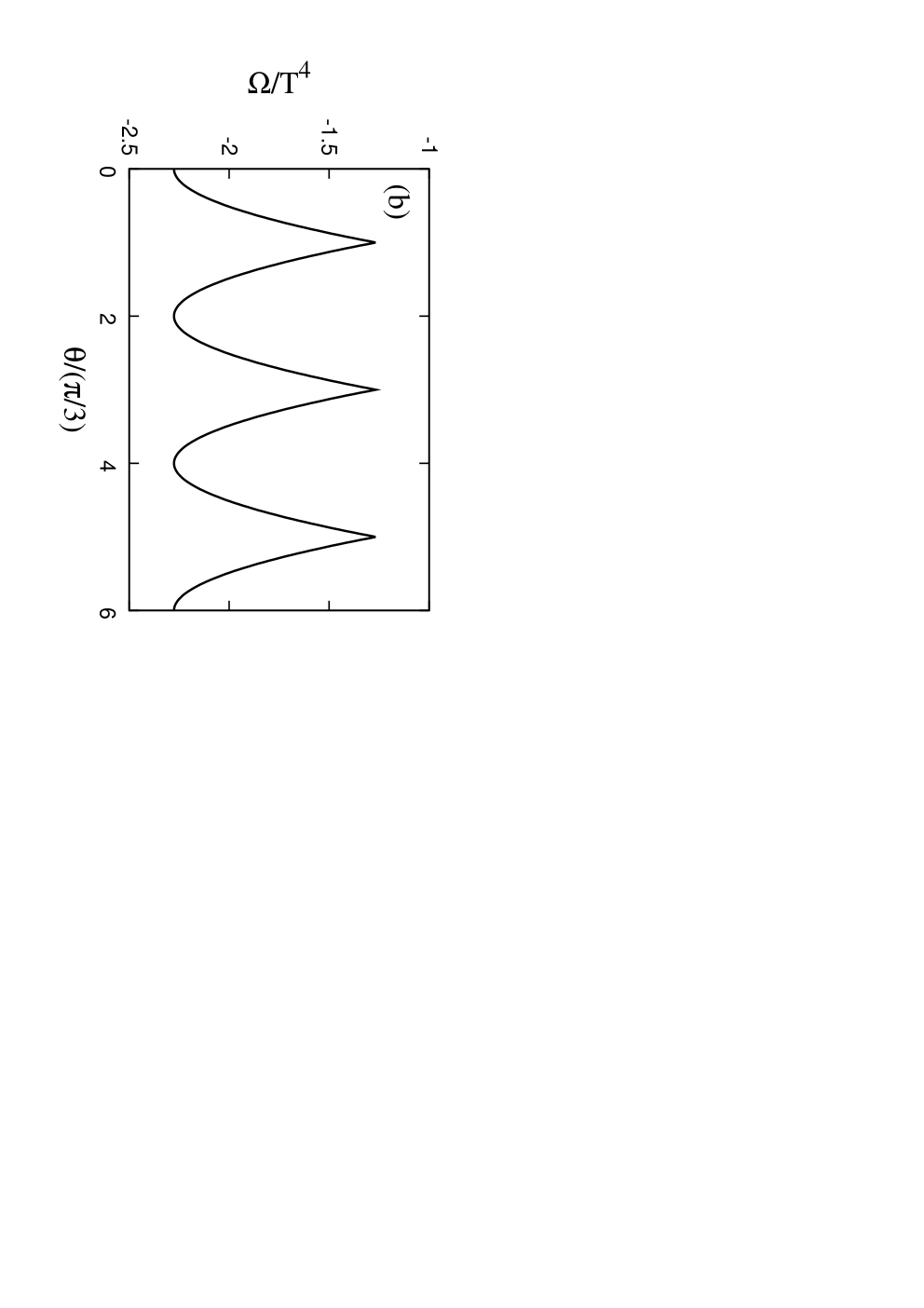
The analyses above based on perturbation are essentially the same as Roberge and Weiss did with perturbative QCD within its one-loop approximation [42, 44]. Actually, the one-loop solutions agree with $\Omega_{k}^{\rm ther}(\theta)$ ($k=0,\pm 1$) of Eq. (39). Thus, at high temperature, the system has three ${\mathbb{Z}}_{3}$ vacua, and they appears alternatively as $\theta$ varies from 0 to $\pi$. This is the RW mechanism, and when $\theta=0$ the system belongs to one of the ${\mathbb{Z}}_{3}$ vacua.

The RW mechanism appears also in the full PNJL calculation free from perturbation. However, the situation is more complicated as shown below. The stationary conditions (11) give three sets of solutions, $\sigma_{k}$ and $\Phi_{k}=|\Phi_{k}|e^{i\phi_{k}}$ ($k=0,\pm 1$), as expected. Inserting the solutions into Eq. (14), we have three solutions $\Omega_{k}$. Figure 8 shows $\theta$-dependence of $\Omega_{k}$ and $\phi_{k}$ in the case of $T=400$ MeV. Surely, there exist three kinds of solutions. At each $\theta$, however, at least one of the three disappears; the solution $\Omega_{0}$ vanishes in the region of $0.53\pi<\theta<1.46\pi$, and the region is shifted by either $2\pi/3$ or $-2\pi/3$ for other solutions. Whenever $\Omega_{k}$ exists, $\phi_{k}$ is about $2\pi k/3$ almost independently of $\theta$, while $|\Phi_{k}|$ depends on $\theta$. The ground state $\Omega_{\rm GS}$ is composed of $\Omega_{0}$ in region (I) $-\pi/3\leq\theta\leq\pi/3$ (mod $2\pi$), $\Omega_{-1}$ in region (II) $\pi/3\leq\theta\leq\pi$ (mod $2\pi$), and $\Omega_{1}$ in region (III) $-\pi\leq\theta\leq-\pi/3$ (mod $2\pi$).