Scrutinizing single-qubit quantum channels: Theory and experiment with trapped ions
Abstract
We report experimental implementation of various types of qubit channels using an individual trapped ion. We analyzed experimental data and we performed tomographic reconstruction of quantum channels based on these data. Specifically, we studied phase damping channels, where the damping acts either in the -plane of the Bloch sphere or in an arbitrary plane that includes the origin of the Bloch sphere. We also experimentally realized and consequently analyzed quantum channels that in addition to phase damping affect also a polarization rotation. We used three reconstruction schemes for estimation of quantum channels from experimental data: i) a linear inverse method, ii) a maximum likelihood estimation, and iii) a constrained maximum likelihood estimation. We took into account realistic experimental conditions where imperfect test-state preparations and biased measurements are incorporated into the estimation schemes. As a result we found that imperfections present in the process of preparation of test states and as well as in measurements of the considered ion trap system do not limit the control of the implementation of the desired channel. Even imperfect preparation of test state and subsequent measurements still provide sufficient resources for the complete quantum-channel tomography.
pacs
03.65.Wj, 03.67.Lx,I Introduction
Any measurement on a physical system gives a result with limited accuracy and precision. This property comes from the fact that the number of data gained by real physical measurements is finite and, moreover, the measurements are influenced by errors and imperfections of the experimental setup. Nevertheless, it is the role of a physicist to interpret measured data and to conclude about properties of the system as reliably as possible.
Determining the action of an unknown quantum channel by quantum process estimation enables us to protect and optimally exploit quantum systems for communication purposes and also for quantum computation by designing efficient schemes correcting errors introduced by the noise (see for instance [1, 2]). Furthermore, for quantum computing it is vital to characterize and improve the experimental performance of quantum logic gates. Quantum process estimation is needed here to first identify imperfections and decoherence. The knowledge of such imperfections then allows us to find remedies for these usually unwanted effects.
Any reconstruction of a quantum channel channel can be viewed as a black-box problem. The black box (quantum channel) is probed by test states. At the input these states are specifically prepared while at the output are specifically measured. Based on the correlations between preparations and measurements one can reconstruct the action of the quantum channel under consideration. In this article we investigate how to reconstruct the action of various engineered quantum qubit channels even in the presence of imperfect initial state preparation and imperfect detection. We shall employ two reconstruction schemes which lead to the same result for “good” data. The first of these reconstruction schemes is the inverse method. In some cases this approach can result an unphysical estimation of the channel (e.g., the estimated channel is not completely positive). Small deviations from the physically valid region are acceptable, because they can be understood as an evidence of finite statistics. In this case the observed frequencies of specific outcomes of measurements are not perfectly compatible with probabilities as predicted by quantum theory, but we can use the maximum likelihood method [3, 4, 5] in order to perform the reconstruction. By construction, the maximum likelihood method always leads to a physical result. If the violation of the physical constraints is large, then the data are apparently biased by some kind of systematic errors, or imperfections in the experimental setup.
I.1 Description of qubit channels
Within the framework of the quantum theory quantum channels are described by completely positive trace-preserving linear maps acting on the system’s state space . For qubits consists of operators where is a real vector with , is a vector of Pauli operators, and represents the identity operator. Therefore, the qubit states can be illustrated as points inside the so-called Bloch sphere formed by Bloch vectors . In this Bloch-sphere representation quantum channels are described as affine transformations of Bloch vectors, i.e.
| (1) |
where is a real matrix and is a translation [6]. In particular, and . Consequently, 12 real parameters need to be determined in order to completely specify a qubit channel .
According to [6] each qubit channel is unitarily equivalent to a specific quantum channel with diagonal matrix . In particular, , where are suitable orthogonal rotations associated with unitary channels , i.e. gives Bloch vector transformation . The diagonal values are the so-called singular values of . If , then the channel is called unital. In our analysis we shall be interested in a special subclass of unital channels - phase damping channels characterized by the relation .
The affine form guarantees that for all matrices and vectors the resulting affine map is trace-preserving. Unfortunately, the analytic conditions of complete positivity are not simple and illustrative [6]. The complete positivity is equivalent to positivity of the state , where stands for the identity channel and is a projection onto a vector describing two-qubit maximally entangled state. If a qubit channel is completely positive, then for all combinations of pluses and minuses. Hence, for phase damping channels .
There are many different experimental procedures how to determine all channel parameters [2, 7, 8, 9, 10, 11]. In general, such an experiment consists of three steps:
- i)
-
preparation of a test state;
- ii)
-
application of an unknown channel;
- iii)
-
measurement of the transformed system.
In principle, the preparation stage can result in a correlated state of a composite system of the system and some ancilla. In this case the experimental arrangement is such that the ancilla is not directly affected by the quantum channel, but the measurement is performed on the whole system. However, this procedure is itself an experimental challenge, and from the experimental point of view, ancilla-free preparations are preferable.
In what follows we shall consider only ancilla-free experiments. By measuring the correlations between the channel inputs and outputs we can determine the channel action and identify the corresponding affine mapping . The linearity of implies that for the purposes of the complete-channel tomography it is necessary to use a collection of linearly independent test states spanning the whole state space. In particular, since for a qubit the linear span of the state space is four-dimensional it follows that at least four test states are necessary.
An important assumption of the above model of the experiment is that the test states are perfectly known, i.e., their preparation is under complete control. That is experimental imperfections (arbitrarily small) in preparation of the desired test states must be included into the description of the test states. If this is the case, then the channel tomography reduces to state tomography of the output states.
This paper is organized as follows: in Section II we shall describe the experimental implementation of the single-qubit channels and describe the measured experimental data. In Section III we shall discuss different strategies for complete channel reconstruction. In Sections IV, V, and VI the tomography of channels using different reconstruction schemes is presented. Results and observations are summarized in Section VII.
II Description of the experiment
In this section the physical realization of various types of quantum channels is described. These include phase-damping channels acting in the x-y-plane of the Bloch sphere where the amount of damping is varied by changing the amplitude of added noise. In addition, phase damping in an arbitrary basis is exemplified by a quantum channel where the damping acts in a plane cutting through the Bloch sphere spanned by the vectors and . Furthermore, combinations of phase damping and polarization rotating channels are implemented with varying rotation angles. A representative subset of these channels have been chosen for detailed reconstruction that is presented in Section III.
The above mentioned quantum channels have been realized experimentally using two hyperfine states of the electronic ground state of an individual electrodynamically trapped 171Yb+ ion as a qubit (, ) [12, 13, 14, 15] and exposing this qubit to unitary operations as well as engineered irreversible dynamics.
In order to take an individual data point that contributes to the characterization of a quantum channel we proceed as follows:
- i)
-
The ion is laser cooled.
- ii)
-
The qubit is initialized in the state .
- iii)
-
The desired input state for testing the quantum channel is prepared. This is either one of the eigenstates of ( are the Pauli matrices, ) with positive eigenvalue (“spin up”), or the eigenstate of with negative eigenvalue (“spin down”).
- iv)
-
The qubit is subjected to the action of the quantum channel.
- v)
-
The qubit is measured in a predetermined basis (). Below, in Section II.1.2, it is shown how the effect of a difference in the detection efficiencies for states and , respectively can be canceled by measuring , but also .
For a given set of parameters characterizing the quantum channel the sequence i)-v) is then repeated for all combinations of test states [prepared in the step iii)] and measurements [chosen in the step v)]. Then one parameter of the quantum channel is changed and all preparation and measurement steps described so far are repeated for this changed set of parameters. Finally, the complete sequence is repeated between 100 and 500 times that allows us to extract from these measurements relative frequencies . Here the index indicates that a measurement in direction has taken place when the initially prepared state was , . The superscript indicates the outcome of a measurement . The notation introduced here for the frequencies allows for a compact description. Note that not all possible combinations of test states and measurement directions are realized experimentally. It is sufficient to prepare four different test states as described in the step iii) above.
In the remainder of this section the initial preparation of the qubit before exposing it to the action of the quantum channel, the measurement in an arbitrary basis, the final read-out, coherent operations and controlled addition of noise are briefly reviewed.
II.1 Physical realization of quantum channels
II.1.1 The qubit and its initialization
The experimental setup used here for a quantum-process estimation has been described elsewhere [13, 14] and a brief summary should suffice: The quantum mechanical two-state system used as a qubit is the S1/2 ground-state hyperfine doublet with total an angular momentum of a single 171Yb+ ion confined in a miniature Paul trap (the diameter of 2 mm). The transition with Bohr frequency is driven by a quasi-resonant microwave (mw) field with an angular frequency near GHz. A static magnetic field is applied to the ion such that the three Zeeman states of the S1/2, F=1 manifold are split by about 6 Mhz. The unitary dynamics of the qubit driven by microwave radiation is virtually free of decoherence, i.e. transversal and longitudinal relaxation rates are negligible [12, 13, 14].
Illuminating the ion with laser light near 369,5 nm, generated by a frequency-doubled Ti:sapphire laser, exciting the S1/2(F=1) P1/2(F=0) resonance serves for initial state preparation in state while photon-counting resonance fluorescence on the S1/2(F=1) P1/2(F=0) transition driven by light near 369 nm allows for a state-selective detection of the qubit. Optically pumping the ion into the metastable level via the P1/2 state is prevented by illumination with light near 935 nm of a diode laser that retrieves the ion to the ground state via the , =, excitation [16]. Laser cooling of the ion is achieved by simultaneously irradiating the ion for 20 ms with laser light near 369 nm and 935 nm and mw radiation where the latter is resonant with the transition. This is done before initializing the ion into state : upon turning the microwave radiation off the ion is then optically pumped into state with probability in the experiments reported here [15].
II.1.2 Measurement of the qubit state
To detect the state of the ion it is irradiated with laser light near 369 nm for a duration of 2 ms. If the ion is in the S1/2(F=1) state, on average photons are registered during that time interval. Due to stray light and dark counts on average photons are registered, if the ion is in the S1/2(F=0) state. In both cases the numbers of registered photons follow a Poissonian distribution. If more than one photon is registered during the counting interval the ion is assumed to be in the S1/2(F=1) state, and if one photon or less is registered the state is assumed to be S1/2(F=0). The probability to detect the S1/2(F = 1) state correctly is and the probability to detect the S1/2(F=0) state correctly is [13]. This implies that the two outcomes are associated with positive operators
| (2) | |||||
| (3) |
The detection efficiencies for both states are not equal, which if not taken into account adds a slight systematic bias to the measurement results. This bias is avoided, if for each measurement in one direction also the measurement in the opposite direction is taken. This means that when, for example, the direction is to be measured, also the direction is measured. Such an “inverted” measurement is described by positive operators
| (4) | |||||
| (5) |
Therefore, combining both measurements into a single one (with equal probability) and identifying the pairs of outcomes and will form a new measurement of the direction associated with positive operators
| (6) | |||||
and
| (7) |
where .
As already defined above, we denote by the frequencies of outcomes for measurements in the direction provided that the test state was used. Then, for the frequencies of measurements we obtain
| (8) |
with .
A measurement in a given direction is performed in two steps: First, a unitary transformation of the qubit is performed (Sec. II.1.3) effecting a rotation of the desired measurement axis onto the z-axis. Second, the qubit is irradiated for 2 ms with laser light resonant with the S1/2(F=1) P1/2 transition and scattered photons are detected, if the state is occupied.
In summary, collecting data in the described way results in the implementation of the measurements described by POVM elements
| (9) |
where we used the fact that are the projectors onto the eigenvectors of associated with eigenvalues .
II.1.3 Coherent operations
Coherent operations on the qubit are achieved by applying near-resonant microwave radiation with the angular frequency driving the magnetic dipole transition between the states and . In the reference frame rotating with , after applying the rotating wave approximation, the time evolution operator determining the evolution of the qubit exposed to linearly polarized mw radiation reads . Here, the Rabi frequency is denoted by and is the detuning between the qubit and the applied radiation. A desired state characterized by a nutation angle and an azimuthal angle on the Bloch sphere is prepared by driving the qubit initially prepared in the state with mw pulses with appropriately chosen detuning , the Rabi frequency , and the duration , and by allowing for a free precession for a prescribed time : Since the applied mw radiation is slightly detuned from the qubit resonance near 12.6 Ghz, the qubit acquires a phase relative to the driving field. Note that when waiting integer multiples of the time needed for a full precession of the Bloch vector in the -plane.
Typical values in these experiments were and . These parameters were determined by recording Rabi oscillations over 2–4 periods and by performing a Ramsey-type experiment with mw pulses separated in time. Also, a Ramsey experiment served to establish the coherence time of the qubit (i.e., the lifetime of the off-diagonal elements of the density matrix describing the qubit, often termed time) that was found to be well over one second [14].
II.1.4 Phase damping
Magnetic field noise may be applied during a prescribed time to the qubit in order to induce phase damping, that is, decay of the off-diagonal elements . After preparation of the input state, a small noisy magnetic field is superimposed onto to the static field that defines the quantization axis. For this purpose an additional magnetic field coil is placed near the trapped ion and is fed by a signal generator producing (nearly) white noise with a Gaussian amplitude distribution. The bandwidth of this additional noise field is limited by a first-order filter with cut-off frequency Hz. Its amplitude is experimentally controlled using a variable attenuator.
The resonance frequency of the qubit when exposed to a magnetic field is derived using the Breit-Rabi formula [17, 18] as
| (10) | |||||
where the hyperfine splitting in zero magnetic field is denoted by , the scaled magnetic field is given by
| (11) |
the total applied magnetic field is denoted by , and indicate the electron and proton masses, respectively, and are the electronic and nuclear g-factor, and is the Bohr magneton.
The scaled magnetic field consists of two parts, and such that to the lowest order in
| (12) | |||||
and . During the free precession of the qubit its dynamics is governed by the Hamiltonian
| (13) |
and after transforming into a rotating frame using the qubit’s state evolves according to
| (14) |
with [19]
| (15) |
The magnetic field fluctuations obey a Gaussian distribution. Thus, , , and also are distributed according to a Gaussian function. When measuring a single instance realization of the qubit after time , the off-diagonal element reads and repeating such a measurement many times amounts to averaging over many realizations of .
The above considerations are valid as long as the correlation time of the noise field is much shorter than the time during which the noise field is applied which is always the case in the experiments presented here. Analytical and numerical calculations on the dephasing of a qubit exposed to Gaussian low-frequency noise are reported by Rabenstein et al. [20]. Their results are applicable to our experiment when setting their qubit tunnel amplitude, to zero ( corresponds to the Rabi frequency in our experiment which is zero while the noisy magnetic field is applied). Rabenstein et al. obtain in the long-time limit () for the damping factor of the off-diagonal elements . Here is the spectral density at zero frequency of the applied Gaussian noise.
As the bandwidth of the noise magnetic field is much smaller than the Zeeman splitting of the state, the ionic state follows this additional field adiabatically and transitions between different Zeeman states are not induced by this noise field.
II.1.5 Data representation
A quantum channel , i.e. the propagation of a qubit between the initial preparation and the final measurement, is in general characterized by 12 real parameters forming a matrix and vector . In the case of ideal preparations and measurements, i.e. and , the frequencies
and, therefore
| (16) | |||||
| (17) |
Note that inserting “bare” frequencies directly into Eq. (16) to calculate the matrix elements and vector elements is not justified when experimental imperfections occur.
Nevertheless we shall use the matrix
| (18) |
and the vector
| (19) |
to represent the experimental data. Only if the test states are pure and the measurements are sharp (i.e., ), then and . Otherwise, the correct interpretation of frequencies lead to different values of channel parameters , . The precise and correct reconstruction relations shall be presented and discussed in Section III.2.
In conclusion, for an experimentally realized quantum channel, the experimental data before applying the appropriate channel reconstruction procedures are represented in the form of a matrix
III Complete channel tomography
In this section we shall describe several ways how to process the experimental data. The experimental data are always presented as frequencies of occurrences of particular experimental outcomes. Ideally, the frequencies are equal to probabilities predicted by the theory. Strictly speaking, this is true if the number of runs of the experiment is infinite. Otherwise, we must deal with statistical errors that can be eliminated by employing specific statistical procedures. The goal of any channel-estimation procedure is to reliably identify (given a specific figure of merit) the channel that is compatible with the measured data.
III.1 Description of methods
III.1.1 Inverse linear method.
Let us assume that statistical errors are vanishingly small, i.e. the frequencies are exactly equal to the probabilities that are going to be compared with predictions of the quantum theory. In the quantum theory the relation between the channels and probabilities is linear and invertible. However, the exact form depends on particular parameters of the experiment, i.e. on a collection of test states and measurements. We shall discuss the details later in Section III.2.
By definition of the procedure the estimated channel is a linear map and its Bloch sphere parametrization guarantees it is also trace-preserving. One may think that experimental results must always give a mapping that is completely positive. However, this is not necessarily the case. As we shall see the experimental data processed in this way can indeed violate the complete positivity constraint. If the experimental conditions are not affected by some systematic errors, then this could happen only if the measured statistics is not sufficiently large.
A naive method how to regularize the statistics is to add white noise into the measured data. Let us denote by the contracting channel maps of all input states into the maximally mixed state , i.e. and . Addition of the white noise channel corresponds to a substitution . For many values of the mapping is completely positive although is not. It is natural to fix the largest possible as the value of this correction parameter and consider to be the “regularized” estimation of the map. This type of regularization catches some important features of the original map, but, in general, this method is not justified by any statistical reasoning. It can be used as a fast test of the quality of the experimental data.
III.1.2 Maximum Likelihood method.
In this approach we do not interpret frequencies as probabilities, but instead we directly process the measured frequencies to estimate the channel. The maximum likelihood method is a general estimation scheme [3, 2] that has already been considered for reconstruction of quantum channels. It has been studied by Hradil and Fiurášek [4], and by Sacchi [5].
It is natural to understand an experiment as a collection of settings representing the choice of the test state and of the measurement . Each measurement apparatus is described by a positive operator valued measure (POVM) determining the positive operators such that . The index runs over all possible outcomes of the measurement . The observed frequencies are calculated as the the fraction of the number of “clicks” (events) associated with and of the number of experiments in which the setting was used. Let us note that . For a given setting , the quantum theory predicts the probabilities
| (24) |
The likelihood functional is defined by the formula
| (25) |
The aim is to identify a physical map that maximizes this function, i.e.
| (26) |
If the maximum is searched only among the (physically relevant) quantum channels, then the complete positivity is guaranteed. In such case, the maximum likelihood method cannot result in an unphysical mapping . Since the complete positivity constraints are complicated even for single-qubit channels the maximum likelihood optimization problem is, in general, complicated. Therefore complex numerical methods must be employed.
As this variational task is usually performed numerically, a question may arise, how to decide, if one has found a global or a local minima. Unfortunately, there is never a certain answer for this question. For proper data a good hint is the actual maximal value of found during the optimization. For a given amount of experimental data a value different in orders of magnitude from other, similar results is suspicious. Also, from the construction of the experiment one has an expectation for the actual result (e.g. phase-damping channel).
For data, which (by the standard reconstruction method described in the previous Section) lead to a proper physical reconstruction, the maximum likelihood gives identical results. Also, as the resulting operation in general is not on the border of the set of the CP channels, the CP condition can be obeyed during the maximization procedure, which speeds up the algorithm dramatically.
For data leading to unphysical results (using the inverse method) the situation is more complicated. The best physical result is normally on the border of the set of CP channels, so one has to take the CP condition into account during the whole procedure. Moreover, the resulting value of might vary significantly depending on how much would the complete operation be non-CP. So the only way for checking the result is the comparison with the expected type of a quantum channel.
III.2 Data processing and interpretation of results
In order to properly interpret the measured experimental data we need to take into account the experimental imprecisions leading to imperfection of the preparation process and also the imperfections in the implementation of sharp measurements . In fact, the latter imperfections must be taken into account also in the specification of the preparation process.
Let us express the states
| (27) |
corresponding to an imperfect preparation of eigenstates of operators . In our particular experiment we use only four of these states . As it was described in Section II.1.2 the systems are measured by one of three observables described by positive operators
| (28) |
where are eigenstates of corresponding to eigenvalues .
The experiment consists of different settings leading to frequencies that are compared with theoretical probabilities
where we used the definitions , and . The goal of the process reconstruction is to determine 12 parameters and describing the quantum channel in the Bloch representation.
As we already mentioned in the experiment we use only four test states . In such case
| (29) |
where . Similarly,
| (30) |
where . The matrix and vector are fixed by performing the state reconstruction experiments of the input test states . Since the experimental data are presented in the form of the matrix and the vector it follows that
| (31) | |||||
| (32) |
Let remind us that this choice of the data representation is motivated by the property that if the test states are pure [i.e., ] and the measurements are sharp (), then and .
The preparation of the input test states is described by the parameters
| (33) |
where are the observed frequencies for the experiment estimating the test states . Inserting this formula into the expressions for and we find
That is, and are proportional to data matrices determined by the preparation procedures of the test states. Hence the data collected in the estimation of the test states can be conveniently expressed in the same form as the data collected in the case of channel estimation procedure. However, the data set matrix does not have to possess the channel requirements on , i.e. it does not have to be completely positive.
In the considered experiment
and the Bloch vectors of actual test states read
The above vectors are the columns of the matrix . The parameter is determined experimentally and reads . The fidelities of preparation of pure input test states , , , are 0.928, 0.907, 0.909, 0.913, respectively. These particular values shall be used in the process tomography procedure using the formulas given by Eqs.(31) and (32).
IV Phase damping quantum channels
The action of the phase damping quantum channel on the Bloch vector is described by the matrix
| (46) |
with the damping parameter . It reduces the th and th components of the Bloch vector while the th component remains unaffected.
As described in Section II.1.4 a phase damping quantum channel is realized by applying a normally distributed noise magnetic field between the preparation and the measurement stages. This noise field is applied for a duration that equals a multiple of the precession time with an amplitude determined by a variable attenuator. The noise magnetic field changes the precession frequency of the ion by a small random amount and therefore adds noise to the phase of the qubit. Upon averaging over many realizations this reduces the - and -components of the Bloch vector.
The damping parameter describes the amount of phase damping that occurs:
| (47) |
with being the duration for which the noise magnetic field is applied and is the spectral density of the applied Gaussian noise at zero frequency.
In order to vary the damping parameter experimentally, the amplitude of the noise magnetic field is changed while the duration is fixed at for the data shown in Fig. 1. The relative noise amplitude is indicated on the x-axis for each matrix and vector element displayed in Fig. 1. Already in this figure we can see the expected pattern of a phase damping channel. That is, the off-diagonal elements and values of almost vanish, while the element remains almost constant and the values of are exponentially decreasing to zero as the amplitude of the noise magnetic field is increasing: The solid (red) line in Fig. 1 indicates a fit with an exponential decay using Eq. (47) where at a relative amplitude of 0 dB is used as a free parameter and varies according to . Here, indicates the relative noise amplitude indicated in dB in Fig. 1 and the time is fixed at .
The fact that is consistent with the effective initial preparation of the qubit in a mixed state and its imperfect detection. This matrix element is expected to remain unaffected by the applied noise, since the noise doesn’t induce transitions between the qubit states. This indeed is found to be the case.
The error bars shown in Fig. 1 indicate a statistical error originating from a finite number of measurements that go into the determination of the relative frequencies and consequently into the matrix elements calculated according to Eq.(18).
IV.1 Estimation without prior knowledge
For example, for the data set corresponding to dB represented by the fourth bar in each individual graph of Fig. 1,
and the linear inverse reconstruction method using Eq. (III.2) results in the mapping
Since it follows that the whole mapping is not positive, hence the reconstruction gives an unphysical result. We find that this feature of “unphysicality” is typical for all values of . However, this is not entirely unexpected, because phase damping channels are on the boundary between positive and non-positive maps. That is, for each phase damping channel there exists a non-positive linear map which is arbitrarily close to . In fact, in our case the violation of the complete positivity is within the statistical errors. The used statistics is relatively small. Each experiment was repeated 100 times.
Employing the maximum likelihood principle for the data taken at dB that was considered already above we now get
We see that this (estimated physical) mapping is not exactly the phase damping channel (see Fig.2), but the obtained precision is in accordance with the size of the statistical sample.

IV.2 Estimation of the phase damping parameter
So far we reconstructed the quantum channel without using any information on the particular physical model of the the experiment. In this part we shall assume that nontrivial a priori information on the estimated channel is available. In particular, we shall consider the channel described and reconstructed above and assume prior knowledge that the channel describes a pure phase damping channel . Let us note, that the results of Section IV do no entirely justify such an assumption, because the implemented channels are not precisely the phase damping channels. Nevertheless, our goal is to present different methods how to determine the phase damping parameter , which is probably the most interesting parameter of any decoherence evolution, because it illustrates how fast the “quantumness” of a given quantum system is deteriorated.
Firstly, we shall employ the maximum likelihood method constrained to phase damping channels only. In this case the optimization of the likelihood is constrained only to channels , that is,
| (48) |
where .
In the second approach we shall also assume the same form of the channel. Now the parameter reads
| (49) |
for an arbitrary test state . Alternatively, one can replace by any other operator with a vanishing -component of , i.e. orthogonal to determining the decoherence basis. Since the relative statistical error is largest for off-diagonal elements, in order to fix some value of we shall use the average value of and , i.e. .
In Tab. 1 and Fig. 3 we present the estimates of the value of using three methods: i) the average for using the linear inverse reconstruction (compare Section IV.1), ii) the average for obtained from maximum likelihood, and iii) obtained from the constrained maximum likelihood [see Eq.(48)].
| setting | -19dB | -16dB | -13dB | -10dB | -7dB | -4dB | -1dB |
|---|---|---|---|---|---|---|---|
| 0.94 | 0.88 | 0.85 | 0.66 | 0.42 | 0.23 | 0.00 | |
| 0.88 | 0.91 | 0.87 | 0.60 | 0.35 | 0.31 | 0.13 | |
| 0.97 | 0.90 | 0.85 | 0.63 | 0.40 | 0.25 | -0.01 |
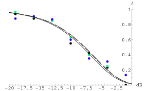
All three methods for evaluation of must give the same value in the limit of infinite statistics (providing that the implemented channels are precisely the phase damping channels). For small statistical samples the first method is, in general, very inappropriate, because it can give even unphysical values. On the other hand the values and can give different values even for infinite statistics. If this is the case, then we must conclude that the phase damping channels are not implemented and the value does not have exactly the desired meaning. In our case the statistical errors in specification of are . Therefore, we can conclude that all three values are approximately the same. Since the differences between and are relatively small (in the context of statistical errors) we can conclude that phase damping channels are realized with quite good accuracy although a precise quantitative specification would require more experimental runs.
V Phase damping quantum channels with change of basis
The phase damping quantum channel shown in the previous paragraph acts in the plane of the Bloch sphere. The phase damping can be applied in a different plane, if the qubit state is rotated prior to application of the noise magnetic field and rotated back afterwards. Here, phase damping in a plane rotated around the -axis spanned by the Bloch vectors with and is examined. For arbitrary , such rotated phase damping is described by the Bloch vector transformation
with the damping parameter as in Eq. (46).
Fig. 4 shows the experimental results for a phase damping channel with varying amplitude of the noise field and fixed . The solid lines indicate a fit of the data using Eqs. (V) and (49) as described above.
As in the previous case, also for this type of channels the basic features are already seen from the data presentation in Fig.4. In contrast to the “pure” phase damping channels shown in Fig. 1, for this channel the off-diagonal elements do not vanish. Furthermore, the z-component is damped. In this set of data the values for and are almost equal because of the particular choice of the rotated basis.
The channel was analyzed in a similar way as the phase damping channel in the previous section. Let us present in detail the reconstruction based on an experiment where the same amount of phase damping was present as in the case of phase damping in the plane, i.e. -10 dB. For the experimental setting -10 dB the data matrix reads
The inverse reconstruction method gives
and the maximum likelihood estimation results in channel
The constrained maximum likelihood method applied to channels of the form (V) results in the estimates on the phase damping rate and the rotation axis angle presented in Tab. II.
| setting | -19dB | -16dB | -13dB | -10dB | -7dB | -4dB | -1dB |
|---|---|---|---|---|---|---|---|
| 32∘ | 32∘ | 24∘ | 42∘ | 41∘ | 43∘ | 44∘ | |
| 0.88 | 0.90 | 0.74 | 0.50 | 0.38 | 0.18 | -0.04 |
In order to fix the parameters experimentally it is sufficient to specify any pair of nonzero elements of the matrix in Eq.(V). For example, we can use as the test state and measure . From the estimated matrix elements the values can be easily calculated. However, in our case we used all the observed values as an input into the constrained maximum likelihood estimation that determines the values of and . As expected, the value of the phase damping rate for dB is in accordance with the corresponding values of in Tab. 1 within the statistical uncertainty.
The correct value (specified by the experimental setup) of the angle is . For weak damping (i.e., small values of added noise and consequently large values of ) the estimated angle deviates from the angle used in the experiment more than for a large damping. However, this deviation is still within the errors of the maximum likelihood estimates that are . The larger deviation when low damping is applied can be rationalized as follows: The fact that the phase damping does not act in the -plane becomes apparent in the increase of the off-diagonal elements and of the matrix only for relatively large damping (compare Fig. 4). For small damping these off-diagonal elements are small with a relatively large statistical error bar, which makes it difficult to accurately estimate for each individual channel the angle by which the plane of phase damping is rotated.
The solid line in Fig. 4 indicates a fit (as opposed to a channel reconstruction) of a given matrix element using Eqs. (V) and (49). Here, the fit includes as a free parameter and takes into account all available results for (i.e., for different strengths of damping) thereby presuming that the channels are characterized by the same angle irrespective of the strength of damping (which indeed was experimentally realized).
VI Polarization rotating and phase damping quantum channels
In a further experiment we combined the phase damping channel with a unitary channel rotating the state space around the axis by an angle . Such polarization rotating channel is realized in our experiment by inserting a pause between the preparation of the qubit and its measurement whose length is a fraction of the precession time . The combined quantum channel realized here propagates the qubit first through a phase damping quantum channel according to Eq. (46) with a relative amplitude of the noise field of -10 dB and then through a phase rotating quantum channel whose rotation angle is varied. The combined action on the Bloch vector is given by the transformation
| (54) |
In Fig. 5 the experimental results for that quantum channel are shown.
One would expect that the zero pause should correspond to the rotation angle for which the diagonal matrix elements are all at their maximum. This is not the case for the data displayed in Fig. 5 where the offset of the phase rotation angle is due to an additional dc magnetic field that was applied simultaneously with the ac noise field.
Tab. III contains the results of the constrained maximum likelihood estimation of the relevant parameters.
| 255∘ | 271∘ | 325∘ | 22∘ | 69∘ | 90∘ | 147∘ | 171∘ | 217∘ | |
|---|---|---|---|---|---|---|---|---|---|
| 0.56 | 0.58 | 0.58 | 0.66 | 0.55 | 0.58 | 0.41 | 0.53 | 0.45 |
Let us note that the values of the damping parameter are in an approximate accordance with the results obtained in the estimations of the previous channels, for which we have seen that the damping parameter for -10 dB is around . In particular, the average gives . Moreover, the rotation angles in the experiment are chosen such that the differences of subsequent angles should be . According to above estimations the average difference is .
VII Conclusion
Quantum process estimation is a necessary tool for characterization of dynamics of physical systems. It can also be used for improvement of efficiency of quantum information processing. We have exposed individual trapped ions to engineered quantum channels and explored various methods for a reconstruction of the action of these channels. This reconstruction takes into account imperfect experimental conditions, namely the imperfect preparation of the test states (that results in a mixed state), a finite detection efficiency and a bias in the detection efficiency for different states.
We have created qubit quantum channels with variable phase damping and fully reconstructed them using the linear inverse method and the maximum likelihood estimate. Alternatively, if it is a priori known that the quantum channel only leads to phase damping, then the estimation of a single parameter is sufficient. In the latter case a constrained maximum likelihood method leads to good results with a minimal number of measurements.
A quantum channel with damping in an arbitrary plane through the Bloch sphere that contains the origin may also be realized and is exemplified here for a particular rotation angle that determines this plane. The full reconstruction of this channel is performed without prior knowledge using the linear inverse and the maximum likelihood methods. Here, too, the maximum likelihood method under constraints gives good results with a significantly reduced number of measurements when prior knowledge about the channel’s action is assumed and used. Furthermore, using the same methods the phase damping accompanied by a polarization rotation is estimated.
The finiteness of experimental statistics affects the precision of our estimates. On average the precision of matrix elements is . From the observed dependence of the phase-damping rate on parameter (see Fig.3) we can determine the constant . In particular, fitting the estimated values of we get .
The implementation of the phase damping channel is based on a clear physical picture based on our knowledge from atomic physics. However, such knowledge is not really used in the complete tomography methods used in this paper. The adopted approach is to consider the experiment as an unknown black box transforming states. Therefore, comparing the estimation with the theoretical expectations gives us nontrivial information about the validity of our assumptions and understanding of the physical situation.
For the constrained maximum likelihood estimation we assume that the channel belongs to a family of phase damping channels characterized by a single parameter. For infinite statistics any difference between unconstrained and constrained maximum likelihood estimations would imply that the model and the experiment do not fit perfectly. Therefore, the distance can provide the quantification of the agreement of the model and the experiment. Let us use as a figure of merit the process fidelity [1]
| (55) |
where and is a projection onto the maximally entangled state. This positive functional equals to unity if and only if the two processes under consideration are the same and it is less than unity (though non-negative) otherwise. For phase damping channels we find that
| (56) |
The value of this fidelity of the channel estimation is very high in spite of imperfect preparations of test states. To be specific, the test states that are not (“ideal”) pure states but rather statistical mixtures that are prepared with the fidelity approximately compared to the ideal test states. Simultaneously, we stress that this imperfect test states are completely known which is a necessary condition for reliable reconstruction of the channel.
The engineered phase damping quantum channels are of particular relevance for quantum information processing. They represent the most destructive type of decoherence, because they are destroying superpositions of logical qubit states that are necessary for the success of quantum computing. Therefore, the controlled implementation of phase damping channels is of use for testing of robustness of quantum computation schemes and error-correction codes.
Acknowledgements.
We acknowledge financial support via the European Union projects QAP 2004-IST-FETPI-15848, HIP FP7-ICT-2007-C-221889, by the projects APVV-0673-07 QIAM, GAČR GA201/07/0603, VEGA-2/0092/09, OP CE QUTE ITMS NFP 262401022, and CE-SAS QUTE, by the Deutsche Forschungsgemeinschaft, and by secunet AG.References
- [1] M.A. Nielsen and I.L. Chuang, Quantum Information and Quantum Computation, (University Press Cambridge, 2000).
- [2] M.G.A. Paris and J. Řeháček, Quantum State Estimation, Springer Series on Lecture Notes in Physics vol. 649, (Springer-Verlag, Berlin, 2004).
- [3] R.A. Fisher, Proc. Cambridge Phil. Soc. 22, 700 (1925).
- [4] J. Fiurášek and Z. Hradil, Phys. Rev. A 63, 020101(R) (2001).
- [5] M.F. Sacchi, Phys. Rev. A 63, 054104 (2001).
- [6] M.B. Ruskai, S. Szarek, and E. Werner, Lin. Alg. Appl. 347, 159 (2002).
- [7] I.L. Chuang and M.A. Nielsen, J. Mod. Opt. 44, 2455 (1997).
- [8] J.F. Poyatos, J.I. Cirac, and P. Zoller, Phys. Rev. Lett. 78, 390 (1997).
- [9] G.M. D’Ariano and P. Lo Presti, Phys. Rev. Lett. 86, 4195 (2001).
- [10] M. Ježek, J. Fiurášek, and Z. Hradil, Phys. Rev. A 68, 012305 (2003).
- [11] J.B. Altepeter, D. Branning, E. Jeffrey, T.C. Wei, P.G. Kwiat, R.T. Thew, J.L. O’Brien, M.A. Nielsen, and A.G. White, Phys. Rev. Lett. 90, 193601 (2003).
- [12] R. Huesmann, Ch. Balzer, Ph. Courteille, W. Neuhauser, and P.E. Toschek, Phys. Rev. Lett. 82, 1611 (1999).
- [13] T. Hannemann, D. Reiss, C. Balzer, W. Neuhauser, P.E. Toschek, and C. Wunderlich, Phys. Rev. A 65, 050303 (2002).
- [14] C. Wunderlich and C. Balzer, Adv. At. Mol. Opt. Phys. 49, 293 (2003).
- [15] C. Balzer, A. Braun, T. Hannemann, C. Paape, M. Ettler, W. Neuhauser, and C. Wunderlich, Phys. Rev. A 73, 041407 (R) (2006).
- [16] A.S. Bell, P. Gill, H.A. Klein, A.P. Levick, C. Tamm, and D. Schnier, Phys. Rev. A 44, R20 (1991).
- [17] G. Breit and I.I. Rabi, Physical Review 38, 2082 (1931).
- [18] A.Corney, Atomic and Laser Spectroscopy, (Clarendon Press, Oxford, 1978).
- [19] S. Brouard and J. Plata, Phys. Rev. A 68, 012311 (2003).
- [20] K. Rabenstein, V.A. Sverdlov, and D.V. Averin, JETP Lett. 79, 646 (2004).