Tests of analytical hadronisation models using event shape moments in $\mathrm{e^{+}e^{-}}$ annihilation

This model [7, 23, 24] is based on the assumption of a non-perturbatively defined strong coupling $\alpha_{\mathrm{S}}(Q^{2})$ which remains finite at and below the Landau pole $\Lambda_{\mbox{\tiny QCD}}$. The Landau pole is the scale where the usual perturbative coupling diverges. The matching scale $Q=\mu_{I}$ , marking the border between perturbative and non-perturbative region, is not uniquely defined. Usually it is taken as $\mu_{I}\simeq 2\,GeV$.

As the non-perturbative coupling cannot be calculated, it is parametrised universally in a simple way by the zeroth moment of the extended coupling over the non-perturbative region,

In first approximation, non-perturbative corrections generate a simple shift of the perturbative differential distribution ${d\sigma_{{}_{\rm NLO}}}/{dy}$ of the event shape variables $1-T$, $C$, $B_{\mathrm{T}}$, $B_{\mathrm{W}}$ and³³ 3 The theoretical calculations are based on the variable $M_{\mathrm{H}}^{2}$ because of the problems with the NLO description of $M_{\mathrm{H}}$ as discussed in [6, 5, 25]. $M_{\mathrm{H}}^{2}$ when relating parton to hadron level,

This prediction is valid only if the value of the event shape variable $y$ is not too large ($y\ll 1$), and the cms energy $Q$ not too small ($Q\gg{\Lambda_{\mbox{\tiny QCD}}}/{y}$). Only the numerical factor $a_{y}$ depends on the event shape variable $y$, see Table 1. However ${\cal P}$ depends on the hard scale $Q$ but is universal for the event shape variables $1-T$, $C$, $B_{\mathrm{T}}$ , $B_{\mathrm{W}}$ and $M_{\mathrm{H}}^{2}$, and has the form [23, 24]

In the $\mathrm{\overline{MS}}$ renormalisation scheme the constant $K$ has the value

with $n_{\mathrm{f}}=5$ at the studied energies, and the beta function coefficient is $\beta_{0}=23/(12\pi)$. The color factors have the values $C_{F}=4/3$, $C_{A}=3$ [26], the Milan factor ${\cal M}$ is known in two loops, ${\cal M}=1.49\pm 20\%$ (for flavour number $n_{\mathrm{f}}=3$ at the relevant low scales). The cited uncertainty results [24] from the estimation of the next order contribution, ${\cal M}_{{}_{\rm NNLO}}={\cal M}_{{}_{\rm NLO}}\cdot(1+{\cal O}({\alpha_{\mathrm{S}}}/{\pi}))$.

Applying the dispersive model calculation (4) of the normalized event shape distribution in definition (1) of the moment of order $n$ and naively neglecting the integration over the unphysical range of negative variable values, gives

The predictions for the moments on hadron level become:

Previous studies [29] indicate that the parameters $\alpha_{\mathrm{S}}(M_{\mathrm{Z^{0}}})$ and $\alpha_{0}(\mu_{I})$ when fitted to $B_{\mathrm{T}}$ and $B_{\mathrm{W}}$ distributions via (4) are not compatible with values derived from $1-T$ and $C$. Therefore improved predictions for these distributions were given. They also describe a compression of the distribution peak, i.e. a narrowing in the two jet region [24, 30]. The non-perturbative factor ${\cal P}$ in the case of $\langle B_{\mathrm{T}}^{1}\rangle$ and $\langle B_{\mathrm{W}}^{1}\rangle$ is replaced by [31]

rsp.

with a rescaled coupling $\widehat{\alpha}_{s}(Q^{2})\equiv\alpha_{\mathrm{S}}({\rm e}^{-3/2}Q^{2})$ and a constant $\eta_{0}\simeq-0.6137$ .

No power correction coefficient has been calculated in the dispersive model for the variable $y^{\rm D}_{23}$. The purely perturbative prediction describes the first moments of $y^{\rm D}_{23}$ well [14, 31]—therefore we also compare it with the higher moments.

The dispersive model gives predictions for several observables and contains only universal free parameters$\alpha_{\mathrm{S}}(M_{\mathrm{Z^{0}}})$ and $\alpha_{0}(\mu_{I})$.

Korchemsky and Tafat [8] describe properties of the event shape variables $1-T$, $C$ and $M_{\mathrm{H}}^{2}$ not included in NLO perturbation theory by a so called shape function, which does not depend on the variable nor the cms energy. This is more general than the dispersive model, as not only a shift of the perturbative prediction is predicted but also a compression of the distribution peak.

The prediction is deduced from studying the two jet region (i.e. $y\ll 1$) in the distribution of the event shape variable $y$. The prediction for the differential distribution is

with a non-perturbative function $f_{y}(\varepsilon)$, dependent on one scale parameter $\epsilon$. This function is derived from the shape function $f(\varepsilon_{L},\varepsilon_{R})$ [8], which depends on two scale parameters $\varepsilon_{L}$, $\varepsilon_{R}$ for the two hemispheres of the event. By the compression of the distribution the validity of the prediction is extended compared to the dispersive model to $y\simeq\Lambda_{\mbox{\tiny QCD}}/Q$.

The shape function can be parametrised [8] by its “first moment”,

its “second moment”,

and a $Q$ dependent function $\delta\lambda_{2}(Q)$. Predictions for the moments of event shape variables can be derived, and $\lambda_{1}$ and $\lambda_{2}$ can be fitted to the data.

From prediction (14) for the distribution of the variables $1-T$, $C$ and $M_{\mathrm{H}}^{2}$, predictions for the mean values follow [8] by integration,

Analogously for the second moments one finds [8],

In this model the more strongly suppressed power corrections have an independent coefficient. The coefficient $\lambda_{1}$ is interpreted as the first “moment” of the shape function, $\lambda_{2}$ the second, and $\delta\lambda_{2}$ as a contribution accounting for the one-hemisphere character of $M_{\mathrm{H}}^{2}$. Therefore these are universal scales.

In [32] the variance of event shape distributions on hadron level was found to be described in the dispersive model perturbatively without significant power corrections. This would open the possibility of an accurate $\alpha_{\mathrm{S}}(M_{\mathrm{Z^{0}}})$ determination.

A theory predicting first and second moments of an event shape variable $y$ also gives a prediction for the variance Var$(y)=\mbox{$\langle y^{2}\rangle$}-\mbox{$\langle y\rangle$}^{2}$, and so a simple prediction for the variance of event shape variables on hadron level is deduced [32] by employing the predictions (7) and (8),

In the dispersive model one obtains a purely perturbative expression for the variance, up to strongly suppressed corrections ${\cal O}({\alpha_{\mathrm{S}}}/{Q^{2}})$.

Predictions for the event shape variance can also be derived from the shape function. The first and second moment predictions (17) and (20) give the identical prediction in case of thrust,

Analogously this follows from (19) and (22) for Var($M_{\mathrm{H}}^{2}$). Var($C$) follows from (18), (21) and the perturbative LO coefficient [20]; up to ${\cal O}({1}/{Q^{2}})$

showing an additional term $\propto\alpha_{\mathrm{S}}/Q$ with coefficient $\lambda_{1}$ as in Subsect. 3.2.

Gardi et al. [9, 10] assume the existence of a reordering of the perturbative series, the so called skeleton expansion [33]—its existence is proven only for abelian field theory like QED. The first contribution to this expansion is a single dressed gluon (SDG) which resums running coupling effects of any order in $\alpha_{\mathrm{S}}$. These are renormalons in the dominant contributions $\propto\beta_{0}^{n}$. The single dressed gluon graphs can be calculated completely. In this way the perturbative prediction $\langle(1-T)^{n}\rangle$_pt. for a moment of thrust can be approximated. This approximated series already diverges and various regularisations differ by definite powers of the cms energy $Q$. These predictions follow:

In general, the non-perturbative correction is predicted as a sum of two terms with different powers in $Q$ and coefficients $\nu_{n}$, $\kappa_{n}$.

The thrust is used in the massless limit,

Here the denominator is changed with respect to the standard definition [6] by ${\sum_{i}|\vec{p}_{i}|}\mapsto{\sum_{i}E_{i}}$, which does not change the thrust value as long as massless partons are considered. Under this change of definition the thrust value calculated with a “massive” virtual gluon is correct, as long as all (massless) partons generated in the hadronisation end up in the same event hemisphere w.r.t. to the thrust axis. This so called “inclusive”calculation is valid only if fragmentation of the gluon is approximately collinear. The perturbative SDG predictions for the moments of thrust are given as perturbation series in the coupling $\bar{a}$ [10], which relates to $\alpha_{\mathrm{S}}(\mu_{R}^{2})$ in the $\mathrm{\overline{MS}}$ scheme by a simple shift of the Landau Pole⁴⁴ 4 In particular the beta function coefficients $\beta_{i}$ have the same values as in the $\mathrm{\overline{MS}}$ scheme.,

The perturbative coefficients are given in so called log moments $d_{i}$ of the characteristic thrust function. The first six log moments for $\langle(1-T)^{1}\rangle$…$\langle(1-T)^{4}\rangle$ were calculated by numerical integration [10]. The perturbative prediction of $\mathcal{O}(\bar{\alpha}_{\mathrm{S}}^{6})$ in the (obviously incomplete) SDG approximation has the form [34]

where the $n$-dependent $d_{i}$ are taken from [10]. Higher order contributions from the running of the coupling are accounted for up to sixth order. Reference [10] gives the prediction explicitly in ${\cal O}(\bar{a}^{3})$ without the term $\beta_{1}d_{1}\pi^{2}\cdot\bar{a}^{3}$. This term with marked effect on the $\bar{a}^{3}$-coefficient results from considering the usual QCD beta function [34]. The symbols $\beta_{0}$…$\beta_{3}$ denote the usual beta function coefficients [35, 36], $\beta_{4}$ is unknown. We set $\beta_{4}$ to 0.

The SDG approximation (26) is complete in leading order ${\cal O}(\bar{a})$ by construction [10]. In higher orders this approximation only gives the terms $\propto\beta_{0}$. Therefore we use the numerically calculated [20] NLO coefficients. For the third and higher orders we employ the SDG approximation,

As the perturbative expansion is an asymptotic (divergent) series [22], the terms are expected to become smaller up to a certain order, and then become larger again. It is of interest

• •

  at which expansion order this happens,

• •

  how the measured coupling depends on the maximum expansion order,

• •

  how the leading power correction $\nu_{n}/Q^{l_{n}}$ depends on the maximum expansion order,

• •

  how the minimum perturbative term relates to the power correction.

The best approximation of the theory by an asymptotic series is expected when truncating it near the minimal term—including additional terms does not necessarily result in a better approximation. Therefore we study the analysis as a function of the truncation order.

Our test uses the first five moments of $1-T$, $B_{\mathrm{T}}$ , $B_{\mathrm{W}}$ , $C$ and $y^{\rm D}_{23}$, and the second and fourth moment of $M_{\mathrm{H}}$. We compare the prediction with the hadron level data, varying two parameters $\alpha_{\mathrm{S}}(M_{\mathrm{Z^{0}}})$ and $\alpha_{0}(\mu_{I})$. Figs. 1, 2 show the comparison of data and predictions (7…11) in the case of $1-T$ and $B_{\mathrm{W}}$. The $\chi^{2}/\mathrm{d.o.f.}$ values—calculated from the statistical errors only—vary between 2 and 10, but should be regarded as being indicative only. Experimental differences between JADE and OPAL contribute significantly to the $\chi^{2}/\mathrm{d.o.f.}$ values. At low cms energies the predictions drop off again—this unphysical behaviour (not always visible in the figures) substantially contributes to the high $\chi^{2}/\mathrm{d.o.f.}$ values.⁵⁵ 5 The case of $y^{\rm D}_{23}$ where we compared with the purely perturbative NLO prediction is different. The energy evolution of the data appears consistent with the prediction but the measured higher moments at 14 GeV are too low. A suitable power correction would scale with a higher power of cms energy, and indeed power terms $\ln\,Q/Q^{2}$ and $1/Q^{2}$ are expected [7] and describe $y^{\rm D}_{23}$ distributions better [38]. The moments of the one-hemisphere variables $B_{\mathrm{W}}$ and in particular $M_{\mathrm{H}}$ are described better than in the respective comparison with hadronisation correction by Monte Carlo models [5].

To estimate the experimental systematic uncertainties, the fits are repeated based on the minimum overlap assumption [5] for combining the OPAL and JADE systematic errors.⁶⁶ 6 The $\chi^{2}/\mathrm{d.o.f.}$ values from these fits are substantially lower than those from the fits employing the statistical errors.

We study uncertainties of theory parameters by the following variations

• •

  The renormalisation scale uncertainty (i.e. the effect of higher perturbative orders) is estimated by setting $x_{\mu}=0.5$ and $x_{\mu}=2.0$. Our default is always $x_{\mu}=1$.

• •

  The hadronisation uncertainty is estimated by setting

  • –

    ${\cal M}=1.49\pm 20\%$,

  • –

    $\mu_{I}=1$ GeV and $\mu_{I}=3$ GeV. The resulting deviations are included into the $\alpha_{\mathrm{S}}(M_{\mathrm{Z^{0}}})$ uncertainty only, as $\alpha_{0}(\mu_{I})$ depends on $\mu_{I}$ directly by its definition (3).

Tables 3 and 4 and Fig. 3 contain the $\alpha_{\mathrm{S}}(M_{\mathrm{Z^{0}}})$ and $\alpha_{0}(\mu_{I})$ results from the standard measurement of the moments of the six event shape variables⁷⁷ 7 We list only results from moments that do not show problems in the multi jet region dicussed below., and from the $x_{\mu}$, $\mu_{I}$ and ${\cal M}$ variations. The values of $\alpha_{\mathrm{S}}(M_{\mathrm{Z^{0}}})$ and $\alpha_{0}(\mu_{I})$ measured from $\langle(1-T)^{1}\rangle$, $\langle C^{1}\rangle$, $\langle B_{\mathrm{T}}^{1}\rangle$, $\langle({y^{\rm D}_{23}})^{1}\rangle$, $\langle M_{\mathrm{H}}^{2}\rangle$ are in agreement within errors with previous analyses, see [31, 39] and references therein. The $\alpha_{\mathrm{S}}(M_{\mathrm{Z^{0}}})$ value from $\langle B_{\mathrm{W}}^{1}\rangle$ is lower and the $\alpha_{0}(\mu_{I})$ value higher than in previous analyses because of the incomplete description of $\langle B_{\mathrm{W}}^{1}\rangle$ in NLO discussed below. This incompleteness affects the predictions at low centre-of-mass energies, leading to high $\alpha_{0}(\mu_{I})$ values and low $\alpha_{\mathrm{S}}$ values. Low energy data have not yet been analysed with a statistics comparable to ours.

The $\alpha_{\mathrm{S}}(M_{\mathrm{Z^{0}}})$ results are similar to those in the analysis employing Monte Carlo models for hadronisiation correction [6, 5]. In particular the $\alpha_{\mathrm{S}}(M_{\mathrm{Z^{0}}})$ values steeply rising with moment order for the variables $1-T$, $C$ and $B_{\mathrm{T}}$ show the incomplete description of the multi jet region in NLO as already seen and discussed in [6, 5]. This is also seen in the large renormalisation scale uncertainties. The $\alpha_{0}(\mu_{I})$ and $\alpha_{\mathrm{S}}(M_{\mathrm{Z^{0}}})$ values from the moments $\langle B_{\mathrm{W}}^{n}\rangle$ are not universal but decrease with moment order $n$. We can validate only the explicitely calculated $\langle B_{\mathrm{W}}^{1}\rangle$ prediction.

Based on the statistical errors, the values of $\alpha_{0}(\mu_{I})$ from the $\langle B_{\mathrm{W}}^{1}\rangle$, $\langle M_{\mathrm{H}}^{2}\rangle$ and $\langle M_{\mathrm{H}}^{4}\rangle$ fits are significantly higher than those from $\langle(1-T)^{1}\rangle$, $\langle C^{1}\rangle$ and $\langle B_{\mathrm{T}}^{1}\rangle$. The NLO description of $B_{\mathrm{W}}$ and $M_{\mathrm{H}}$ in the two jet region is rather incomplete compared to $1-T$, $C$ and $B_{\mathrm{T}}$—especially at low energy where the value of the coupling is high. At low $Q$ the NLO predictions of the $B_{\mathrm{W}}$, $y^{\rm D}_{23}$ and $M_{\mathrm{H}}$ distributions are (unphysically) negative in a large range of the two jet region [38, 25]. This incompleteness of the NLO prediction for the moments—in the case of $\langle B_{\mathrm{W}}^{1}\rangle$ the $\alpha_{\mathrm{S}}^{2}$ coefficient is even negative—is compensated by a larger power correction. The perturbative description then contributes less as is seen by the low $\alpha_{\mathrm{S}}(M_{\mathrm{Z^{0}}})$ values. Fits to JADE data of $\langle B_{\mathrm{W}}^{1}\rangle$ alone give $\alpha_{\mathrm{S}}(M_{\mathrm{Z^{0}}})=0.1029\pm 0.0016$, $\alpha_{0}(\mu_{I})=0.728\pm 0.017$; to OPAL alone they return $\alpha_{\mathrm{S}}(M_{\mathrm{Z^{0}}})=0.1242\pm 0.0025$, $\alpha_{0}(\mu_{I})=0.234\pm 0.103$ (statistical errors). So at low energies where the coupling is large, the compensation is stronger, and the power correction is not universal (JADE and OPAL agree better on every other moment).

For averaging $\alpha_{\mathrm{S}}(M_{\mathrm{Z^{0}}})$ and $\alpha_{0}(\mu_{I})$ over many variables and moment orders, we exclude moments that suffer from the problems discussed in the preceding two paragraphs: The deficiencies in the description of the multi jet region for the two-hemisphere variables have already been seen in [6, 5]. To select observables with an apparently converging perturbative prediction, we consider as in [6, 5] only those results for which the NLO term in equation (2) is less than half the corresponding LO term (i.e. $|K|<25$ or $|K\alpha_{\mathrm{S}}/2\pi|<0.5$), with $K=\mathcal{B}_{n}/\mathcal{A}_{n}$. The $K$ values are shown in Refs. [6, 5].

The higher moments of the jet broadenings are excluded because of the incomplete [29] description of their distributions in general. As in [5] the first moment of $B_{\mathrm{W}}$ is excluded because the universality of the fit parameters could not be confirmed.

Thus we combine the results of $\alpha_{\mathrm{S}}(M_{\mathrm{Z^{0}}})$ and $\alpha_{0}(\mu_{I})$ from the moments $\langle(1-T)^{1}\rangle$, $\langle C^{1}\rangle$, $\langle B_{\mathrm{T}}^{1}\rangle$, $\langle({y^{\rm D}_{23}})^{1}\rangle$…$\langle({y^{\rm D}_{23}})^{5}\rangle$, and $\langle M_{\mathrm{H}}^{2}\rangle$, $\langle M_{\mathrm{H}}^{4}\rangle$. The parameters are consistent within total errors, and the combination procedure follows that used in [6, 5].⁸⁸ 8 The covariances of the statistical errors are estimated by PYTHIA at hadron level at 91.2 GeV, the covariances of the experimental systematic uncertainties are taken as$E_{ij}=\mathrm{Min}\{\sigma_{{\rm exp.},\,i}^{2}\,,\;\sigma_{{\rm exp.},\,j}^{2}\}$, and hadronisation and renormalisation scale uncertainties are found by repeating the analysis with varied parameters. The correlations between $\alpha_{\mathrm{S}}(M_{\mathrm{Z^{0}}})$ and $\alpha_{0}(\mu_{I})$ have rather constant values from -0.80 to -0.93 and thus the combination is done individually for $\alpha_{\mathrm{S}}(M_{\mathrm{Z^{0}}})$ and $\alpha_{0}(\mu_{I})$. The averages are

In [8] values for the shape function parameters were determined by comparing a distribution of $M_{H}^{2}$ at 91 GeV with the NLO+NLLA prediction combined with power terms from the shape function to be $\lambda_{1}=1.22\,$GeV, $\lambda_{2}=1.70\,$GeV² and $\delta\lambda_{2}$ from $\delta\lambda_{2}(10$ GeV$)=1.4\,$(GeV)² to $\delta\lambda_{2}(100\,$GeV$)=1.2\,$(GeV)².

We perform fits to the moments $\langle(1-T)^{1}\rangle$, $\langle C^{1}\rangle$ and $\langle M_{\mathrm{H}}^{2}\rangle$ with two free parameters $\alpha_{\mathrm{S}}(M_{\mathrm{Z^{0}}})$ and $\lambda_{1}$. Fits to the higher moments $\langle(1-T)^{2}\rangle$, $\langle C^{2}\rangle$ and $\langle M_{\mathrm{H}}^{4}\rangle$ are done with an additional parameter. Because of the weak energy dependence of $\delta\lambda_{2}$ in (22) we substitute the numerator $\lambda_{2}+\delta\lambda_{2}(Q)$ by the fit parameter $\overline{\lambda}_{2}$. The fits to $\langle C^{2}\rangle$ and $\langle M_{\mathrm{H}}^{4}\rangle$ are not sensitive to the parameter $\overline{\lambda}_{2}$ while the fit to $\langle(1-T)^{2}\rangle$ gives $\overline{\lambda}_{2}=(1.2\pm 1.3$) (GeV)². For further analysis we therefore set $\overline{\lambda}_{2}=0$.

Fig. 4 shows the comparison of the data with the prediction. The data are fitted well with $\chi^{2}/\mathrm{d.o.f.}$—based on the statistical errors—in the order of one. As before, the experimental systematic uncertainties are estimated by the minimum overlap assumption, and the renormalisation scale uncertainty by setting $x_{\mu}=0.5$ and $x_{\mu}=2.0$ .

Table 5 and Fig. 5 contain the results for $\alpha_{\mathrm{S}}(M_{\mathrm{Z^{0}}})$ and $\lambda_{1}$ from the standard measurement and the systematic variations.

The values of $\alpha_{\mathrm{S}}(M_{\mathrm{Z^{0}}})$ show the typical increase for the higher moments of $1-T$ and $C$. The values of $\lambda_{1}$ are consistent for the first two moments of every event shape variable. Furthermore they are consistent for the two-hemisphere variables $1-T$ and $C$. However, the values from $M_{\mathrm{H}}$ are not compatible. As the respective predictions are similar, we refer to the high values of $\alpha_{0}(\mu_{I})$ from the moments $\langle M_{\mathrm{H}}^{2}\rangle$ and $\langle M_{\mathrm{H}}^{4}\rangle$ in the dispersive model, see Subsect. 4.1. The large power corrections compensate for the incomplete perturbative NLO description. Since the values are not consistent and no systematic evaluation of the theory uncertainty is available, we do not combine any of the fit parameters.

The $\lambda_{1}$ values from $1-T$, $C$ and, less pronounced, from $M_{\mathrm{H}}$ are smaller than the results in [8]. A substantial difference of [8] with our work is the inclusion of the NLLA approximation in the distribution prediction, which is not available for the moments.

From the first and second moments of event shape variables $y$ the variance Var$(y)=\mbox{$\langle y^{2}\rangle$}-\mbox{$\langle y\rangle$}^{2}$ has been calculated [40]. The experimental uncertainties have been determined by systematic variations analogously to the moments at hadron level [5, 6]. The variance of $C$, $B_{\mathrm{T}}$, $B_{\mathrm{W}}$, $M_{\mathrm{H}}$ and $M_{\mathrm{H}}^{2}$ becomes larger with rising $Q$ while the variance of $1-T$ becomes smaller, see⁹⁹ 9 In case of $1-T$ this is not seen very clearly in the plot, but significantly in a straight line fit. Fig. 6 and [40]. Studying other observables defined in [6] we find that the variance of $T_{\mathrm{maj.}}$ and $O$ becomes larger with rising $Q$ while the variance of $T_{\mathrm{min.}}$, $S$, $M_{\mathrm{L}}$ and $B_{\mathrm{N}}$ becomes smaller, see [40]. This behaviour is determined by the multi jet region of the distribution [41]. The evolution is reproduced by Monte Carlo models qualitatively well; however data and models differ by typically up to five standard deviations.

Fig. 6 shows the comparison of the prediction (23) using the dispersive model and data of $1-T$, $C$, $B_{\mathrm{T}}$, $B_{\mathrm{W}}$, $y^{\rm D}_{23}$ and $M_{\mathrm{H}}^{2}$. The fits of the free parameter $\alpha_{\mathrm{S}}(M_{\mathrm{Z^{0}}})$ use central values of the measurements and the statistical errors. The energy evolution of prediction and data forVar($B_{\mathrm{W}}$), Var($1-T$), and Var($y^{\rm D}_{23}$) coincides qualitatively (in case of Var($y^{\rm D}_{23}$) except for the lowest energy points of 14 and 22 GeV), but not for Var($C$), Var($B_{\mathrm{T}}$) and Var($M_{\mathrm{H}}^{2}$). The $\chi^{2}/\mathrm{d.o.f.}$ values are large and the $\alpha_{\mathrm{S}}(M_{\mathrm{Z^{0}}})$ values are not compatible with each other or with established QCD analyses.

The predictions using the shape function differ only for Var($C$) from the dispersive model. Fig. 7 shows the comparison of this prediction (24) and data. The fit gives $\chi^{2}/\mathrm{d.o.f.}=50/8$, $\alpha_{\mathrm{S}}(M_{\mathrm{Z^{0}}})=0.0963\pm 0.0004$ and$\lambda_{1}=(0.824\pm 0.025)\,$GeV (statistical errors). The correlation of $\alpha_{\mathrm{S}}(M_{\mathrm{Z^{0}}})$ and $\lambda_{1}$ is 0.80 .

In the shape function description the $Q$ evolution of the perturbative description deviating from the data is corrected at low energies by the term $\propto\lambda_{1}$. Thus the steep energy evolution at low $Q$ is reproduced successfully. However, the fitted values $\alpha_{\mathrm{S}}(M_{\mathrm{Z^{0}}})$ and $\lambda_{1}$ are not compatible with the corresponding values from $\langle C^{1}\rangle$ or $\langle C^{2}\rangle$.

The hadron level data are compared with the five different predictions which result from truncating (27) after order ${\cal O}(\bar{a}^{2})$…${\cal O}(\bar{a}^{6})$. The data are described by the predictions well. Fig. 8 shows the comparison¹⁰¹⁰ 10 Comparisons for second to sixth expansion order, and more discussion, can be found in [41]. of data and prediction for truncating after $\bar{a}^{5}$. The fit results for $\alpha_{\mathrm{S}}$ and $\nu_{i}$ are given in Table 6. The coefficients $\kappa_{2}$…$\kappa_{4}$ of the more strongly suppressed power correction in all instances turn out to be compatible with zero.

For every moment order we study specific properties to find the series describing the data best. The $\chi^{2}/\mathrm{d.o.f.}$ values from the various expansion orders do not differ significantly for any moment order and thus do not discriminate between different expansion orders.

$\langle(1-T)^{1}\rangle$:

For the first thrust moment at the order $m_{\rm max}=5$ the power correction is compatible with zero, then it becomes negative.¹¹¹¹ 11 There is no distinct sign of the power term. It can be positive or negative, or change its sign when using different regularisations [34]. The values of $\alpha_{\mathrm{S}}(M_{\mathrm{Z^{0}}})$ and the power correction reach their minimum at $m_{\mathrm{m}ax}=5$, so the convergence appears best at $m_{\mathrm{m}ax}=5$.

$\langle(1-T)^{2}\rangle$:

Including higher perturbative orders the $\alpha_{\mathrm{S}}(M_{\mathrm{Z^{0}}})$ and $\nu_{2}$ values from the second thrust moment decrease. The purely perturbative description appears continually more accurate, we therefore choose $m_{\rm max}=6$ .

$\langle(1-T)^{3}\rangle$, $\langle(1-T)^{4}\rangle$:

Fitting the third or fourth thrust moment, to compensate the negative perturbative terms the power correction increases when increasing the truncation order. Thus the NLO description appears more accurate than the SDG approximation, and we choose $m_{\mathrm{m}ax}=2$.

Fig. 9 compares the perturbative terms and the power correction terms.

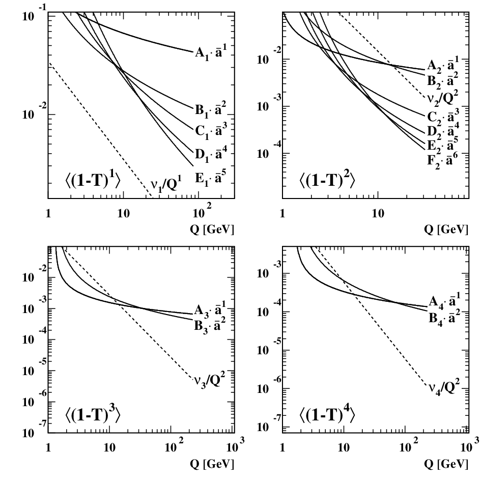
In case of the first moment the power correction is compatible with zero; the purely perturbative prediction from the SDG approximation already describes the data well. The power correction is larger for the third and fourth moments, but is still small compared to the LO and NLO perturbative terms down to $Q=10$ GeV. In case of the second moment the higher SDG terms up to ${\cal O}(\bar{a}^{6})$ are comparable with the power correction.

References

- (1) H. Fritzsch, M. Gell-Mann, H. Leutwyler, Phys. Lett. B 47, 365 (1973)
- (2) D. Gross, F. Wilczek, Phys. Rev. Lett. 30, 1343 (1973)
- (3) D. Gross, F. Wilczek, Phys. Rev. D 8, 3633 (1973)
- (4) H. Politzer, Phys. Rev. Lett. 30, 1346 (1973)
- (5) C. Pahl, S. Bethke, S. Kluth, J. Schieck, Eur. Phys. J. C 60, 181 (2009)
- (6) OPAL Coll., G. Abbiendi et al, Eur. Phys. J. C 40, 287 (2005)
- (7) Y. Dokshitzer, G. Marchesini, B. Webber, Nucl. Phys. B 469, 93 (1996)
- (8) G. Korchemsky, S. Tafat, JHEP 0010, 010 (2000)
- (9) E. Gardi, G. Grunberg, JHEP 9911, 016 (1999)
- (10) E. Gardi, JHEP 0004, 030 (2000)
- (11) ALEPH Coll., A. Heister et al, Eur. Phys. J. C 35, 457 (2004)
- (12) L3 Coll., P. Achard et al, Phys. Rept. 399, 71 (2004)
- (13) DELPHI Coll., P. Abreu et al, Physics Letters B 456, 322 (1999)
- (14) JADE Coll., P. A. Movilla Fernández, S. Bethke, O. Biebel, S. Kluth et al, Eur. Phys. J. C 22, 1 (2001)
- (15) M. Dasgupta, G. Salam, J. Phys. G 30, R143 (2004)
- (16) A. Gehrmann-De Ridder, T. Gehrmann, E. W. N. Glover, G. Heinrich, JHEP 12, 094 (2007)
- (17) S. Weinzierl, Phys. Rev. Lett. 101, 162001 (2008)
- (18) JADE Coll., P. A. Movilla Fernández, O. Biebel, S. Bethke, S. Kluth, P. Pfeifenschneider et al, Eur. Phys. J. C 1, 461 (1998)
- (19) A. Gehrmann-De Ridder, T. Gehrmann, E. W. N. Glover, G. Heinrich, arXiv 0903.4658 (2009)
- (20) S. Catani, M. Seymour, Phys. Lett. B 378, 287 (1996)
- (21) R. Ellis, D. Ross, A. Terrano, Nucl. Phys. B 178, 421 (1981)
- (22) M. Beneke, Phys. Rept. 317, 1 (1999)
- (23) Y. Dokshitzer, G. Marchesini, B. Webber, Phys. Lett. B 352, 451 (1995)
- (24) Y. Dokshitzer, In: High energy physics ICHEP 1998, proceedings of the 29th international conference, 1998
- (25) C. Pahl, arXiv 0810.3326, to appear in High Energy Physics ICHEP 2008, Proceedings of the 34th International Conference (2008)
- (26) R. Ellis, W. Stirling, B. Webber, Cambridge Monographs on Particle Physics, Nuclear Physics and Cosmology 8 (1996), Cambridge University Press
- (27) Y. Dokshitzer, A. Lucenti, G. Marchesini, G. Salam, Nucl. Phys. B 511, 396 (1998)
- (28) Y. Dokshitzer, A. Lucenti, G. Marchesini, G. Salam, JHEP 05, 003 (1998)
- (29) P. A. Movilla Fernández, Nucl. Phys. Proc. Suppl. 74, 384 (1999)
- (30) Y. Dokshitzer, G. Marchesini, G. Salam, Eur. Phys. J. direct C 1, 3 (1999)
- (31) O. Biebel, Phys. Rept. 340, 165 (2001)
- (32) B. Webber, Nucl. Phys. Proc. Suppl. 71, 66 (1999)
- (33) H.J. Lu, C.A.R. Sa de Melo, Phys. Lett. B 273, 260 (1991)
- (34) E. Gardi, Private communication
- (35) T. van Ritbergen, J. Vermaseren, S. Larin, Phys. Lett. B 400, 379 (1997)
- (36) M. Czakon, Nucl. Phys. B 710, 485 (2005)
- (37) JADE and OPAL Coll., P. Pfeifenschneider et al, Eur. Phys. J. C 17, 19 (2000)
- (38)
P. A. Movilla Fernández, Ph.D. thesis, RWTH Aachen (2003). http://nbn-resolving.de/urn:nbn:de:hbz:82-
opus-4836 - (39) S. Kluth, Rept. Prog. Phys 69, 1771 (2006)
- (40) http://durpdg.dur.ac.uk/HEPDATA/
- (41)
C. Pahl, Ph.D. thesis, TU München (2007). http://nbn-resolving.de/urn:nbn:de:bvb:91-diss-
20070906-627360-1-2 - (42) S. Bethke, Prog. Part. Nucl. Phys. 58, 351 (2006)