IPPP/09/21; DCPT/09/42
Tunneling of the 3rd kind
Holger Gies1 and Joerg Jaeckel2
1Theoretisch-Physikalisches Institut, Friedrich-Schiller-Universit¨at Jena,
Max-Wien-Platz 1, D-07743 Jena, Germany
2Institute for Particle Physics Phenomenology, Durham
University,
Durham DH1 3LE, United Kingdom
holger.gies@uni-jena.de
joerg.jaeckel@durham.ac.uk
Abstract
We study a new kind of tunneling of particles through a barrier particular to quantum field theory. Here, the particles traverse the barrier by splitting into a virtual pair of particles of a different species which interacts only very weakly with the barrier and can therefore pass through it. Behind the barrier, the pair recombines into a particle of the original species. As an example, we discuss the case where photons split into a pair of minicharged particles. This process could be observed in experiments of the light-shining-through-a-wall type and may be used to search for minicharged particles in laboratory experiments.
1 Introduction
Tunneling of particles through a potential barrier is a paradigmatic quantum mechanical process [1, 2]. A particle may cross a potential barrier of finite height and thickness because it can penetrate into classically forbidden regions with finite probability in agreement with Heisenberg’s uncertainty principle. Accordingly, the amplitude for the tunneling process is controlled by the Planck constant , the height and width of the potential barrier, .
Field theory with different particle species allows for a different way to penetrate, or more precisely circumnavigate, a barrier. The particle can transmute or oscillate into a different species that does not (or only very weakly) interact with the barrier. Behind the barrier, the particle then reconverts into the original species. This process is depicted in Fig. 1 and forms the basis [3] of so-called light-shining-through-a-wall experiments [4] that can be used to search for axions [3] and other light particles [5, 6]. Since the intermediate particles are real and do not interact with the barrier, height and width of the original barrier do not matter.
In this note we study a generalization of this process allowed by quantum field theory in which the intermediate particle(s) crossing the barrier are not real but virtual. For example, the initial particle could split into a virtual particle-antiparticle pair which then recombines behind the barrier as depicted in Fig. 2. Again, the intermediate particles do not interact with the barrier so the height of the barrier does not matter. The width of the barrier, however, matters because the virtuality of the intermediate particles typically goes along with a characteristic length scale.
As a concrete example of this “tunneling of the 3rd kind”, we study the case of a photon splitting into a pair of particles with a tiny electric charge, so-called minicharged particles, in Sects. 2, 3. The barrier can be thought of as a mirror or, alternatively, an opaque wall. If the charges of the intermediate particles are small enough, these minicharged particles have a tiny cross section with the atoms in the mirror and consequently simply pass through the wall. By contrast, the analogous process with electrons does not work, because electrons, too, would interact with the mirror/wall and would be stopped. Moreover, as we shall see below, for photon frequencies below the mass of the created virtual particles the process is exponentially suppressed. Another possibility within the standard model would be the conversion of the photon into a neutrino–antineutrino pair, for instance, as can be stimulated by a magnetic field, see Fig. 3. But since neutrinos couple to photons only very indirectly, this process is highly suppressed. Therefore, the standard model background for the corresponding light-shining-through-a-wall signal is very small and tunneling of the 3rd kind can serve as a tool to search for physics beyond the standard model in the form of light minicharged particles. The latter arise naturally and consistently11 1 In theories with kinetic mixing [8] minicharged particles are indeed consistent with the existence of magnetic monopoles [9]. in many extensions of the standard model based on field and string theory [8, 10].
A particularly interesting type of experiment to search for a light-shining-through-a-wall effect caused by tunneling of the 3rd kind is the “superconducting box” experiment proposed in [11] in which one searches for magnetic fields leaking into a volume shielded by a superconductor. We will look at this option in Sect. 4.2 and estimate the sensitivity for such an experiment.
2 Setting
Let us identify the ingredients for constructing the transition amplitude and probability for a particle to go through the wall via tunneling of the 3rd kind as depicted in Fig. 2. To be explicit, we concentrate on the case of a photon fluctuating into two minicharged particles. The generalization to other types of particles is, however, straightforward.
Including quantum effects, the effective Lagrangian for a propagating photon is given by:
| (2.1) |
where denotes the two-point correlator, i.e., the vacuum polarization tensor.
The matter in the wall modifies the ‘classical’ first part of the Lagrangian (2.1) by boundary conditions such that the photon classically cannot cross the wall. On the one-loop level, the vacuum polarization tensor (or, more precisely, the contribution generated by the minicharged particles) arises from the loop of minicharged particles shown in Fig. 2. Since minicharged particles interact only very weakly with the matter of the wall, this part of the vacuum polarization tensor remains essentially unaffected by the presence of the wall and allows for a non-vanishing transition amplitude for photons through the wall. In the following, we will calculate the transition amplitude caused by the polarization tensor in the presence of boundary conditions arising from the wall.
If translational invariance holds for the fluctuations (not necessarily for the photon field) the resulting polarization tensor satisfies . Together with the Ward identity, this implies that the polarization tensor can be written in terms of a single scalar function in momentum space,
| (2.2) |
The metric is given by , such that . The equation of motion resulting from Eq. (2.1) for transversal modes reads in momentum space
| (2.3) |
Here and in the following, we drop Lorentz indices, since our considerations are independent of the polarization of the transversal mode. In this work, we consider a set-up where translational invariance is broken for the photon field along the axis. Hence, it is useful to introduce the partial Fourier transforms (),
| (2.4) | |||||
| (2.5) |
in terms of which the equations of motion read
| (2.6) | |||||
In the last step, we have introduced the fluctuation-induced current .
In the present work, we break translational invariance for the photon by a wall of thickness , infinitely extended into the plane. The left side of the wall is put at , the right side extends to . The wall imposes boundary conditions on the photon field. For instance, if the wall is perfectly conducting, a transverse photon propagating along the axis normal to the wall () has to satisfy Dirichlet boundary conditions at the wall’s surface, corresponding to vanishing transverse electric components on the conductor. For a wave packet , the free equation of motion for the left half-space is solved by
| (2.7) |
In absence of any external photon field to the right of the wall , the induced current in this region of space is
| (2.8) |
We observe that the quantum nonlocalities, or loosely speaking, the spatial extent of the fluctuations described by the two-point correlator give rise to a nonvanishing source on the right hand side of the wall.
The solution to the free Green’s function equation,
| (2.9) |
for reads
| (2.10) |
such that the induced outgoing wave to the right of the wall is given by
| (2.11) |
In the present case, the polarization of is identical to that of the incident photon. In Eq. (2.11), we have confined ourselves to the outgoing right-moving far field at . Near the wall, the Green’s function in the presence of the boundary at has to be used instead; the latter in addition contains left-moving components which are of no relevance in the following.
3 Photon transition amplitude
Let us assume the existence of minicharged particles that couple weakly to photons but not directly to matter which the wall consists of. For minimally coupled minicharged Dirac fermions, the well-known results from QED can immediately be taken over. We begin with the well-known representation22 2 In the Appendix, we check our calculation by using the Feynman parameter representation of the polarization tensor. of the polarization tensor in QED, see, e.g., [12], where33 3 Our conventions for differ from those of [12] by an additional factor of .
| (3.1) |
Here, is the analogue of the QED coupling constant including the minicharge , , .
The integral can be done by using the residue theorem, exhibiting two poles: one below and one above the real axis. Since we are eventually interested in the polarization tensor for , we close the contour in the upper half plane and pick up the residue of the corresponding pole. Let us carefully distinguish between the following two cases: For large frequencies, , the pole occurs close to the real axis at
| (3.2) |
For small frequencies, , the pole lies on the imaginary axis,
| (3.3) |
As a result, we obtain for the two cases:
This representation can now be plugged into Eq. (2.12). For simplicity, we confine ourselves to photon propagation parallel to the axis with . For frequencies below threshold, , only the second case occurs; above threshold, both cases contribute. Using the substitutions
| (3.7) |
for the first and second case, respectively, the induced outgoing photon field can be computed from Eqs. (2.8) and (2.11), yielding the representation
| (3.8) |
where we have introduced the dimensionless auxiliary functions
| (3.9) | |||||
| (3.10) |
These auxiliary functions can be numerically evaluated to a high precision with standard routines. Insertion of the result into Eq. (2.12) yields the final tunneling probability,
| (3.11) |
which will be discussed in various limiting cases in the following.
3.1 Small-frequency limit
For all frequencies , we have such that only the function contributes. Rescaling the integration variable such that the lower bound of the integral is unity, the limit reduces to a simpler representation:
| (3.12) |
In the limit corresponding to thick walls compared to the Compton wavelength of the minicharged particle, the asymptotics of the integral can be extracted by a saddle-point approximation, yielding
| (3.13) |
This results exhibits a typical exponential decrease with an exponent which is linear in the wall thickness , as is familiar from quantum mechanical tunneling processes. In Fig. 4, we compare the approximate result, Eq. (3.13), for the transition probability of photons through the wall to an exact numerical evaluation of the integrals. Already for modest values of the wall thickness, , we find reasonable quantitative agreement on the level of .

The analogy to quantum mechanical tunneling becomes even more transparent in the worldline approach to quantum field theory [13]. Here, quantum field theoretic propagators are represented by quantum mechanical path integrals in a fictious time. These paths can be thought of as Lorentz-invariant spacetime trajectories of the quantum fluctuations. In the above limit of small photon frequency and large wall thickness, these path integrals can be approximated semiclassically, resulting in minicharged-particle propagators of the form . As the probability amplitude for our process involves two propagators, the probability (3.13), being the square of the amplitude, decays with .
The important difference to quantum mechanical tunneling is that it is not a wave function of an on-shell particle that penetrates the barrier. Instead, the existence of and the interaction with off-shell intermediate states are necessary to give rise to this new tunneling phenomenon. This is somewhat similar to the tunneling picture of Schwinger pair production [14, 15, 16]: here, the production of charged particles is facilitated by an external electric field that assists fluctuations to tunnel out of the vacuum through the spectral gap to on-shell asymptotic states. Of course, an important difference remains, as there is a clear distinction in our case between the intermediate fluctuation states and the asymptotic photons.
Let us now consider the limit of the wall thickness being small compared to the Compton wavelength of the minicharged particle, . Here, the auxiliary function diverges logarithmically. As this limit probes the vacuum polarization at larger and larger momentum scales, this logarithmic behavior corresponds to the logarithmic running of the gauge coupling above the mass threshold:
| (3.14) |
For instance, for a wall thickness in the millimeter range, this limit applies to minicharged particles with a mass below the meV scale, where the driving photon frequency is chosen even much below the meV scale.
3.2 Large-frequency limit
For larger frequencies , both auxiliary functions and contribute. Here, analytic limits are more difficult to obtain, since cancelations between the two integrals can occur.
For instance, the limit of a large wall thickness can be obtained from expanding in Eq. (3.9) with respect to the upper bound; contributions from the lower bound are canceled by corresponding contributions from , yielding for the probability
| (3.15) |
In the case of small masses, we note that the approximation is valid only at fairly large wall thickness, rendering this limit phenomenologically less relevant.
For not too large , the small-wall-thickness limit is dominated by which reduces to
| (3.16) |
Again, the limit of small wall thickness probes the high-momentum structure of vacuum polarization, yielding a logarithmic increase of the tunneling probability,
| (3.17) |
Note that the mass of the fluctuating particle drops out in this limit.
Of particular phenomenological interest is the limit for . This limit is again purely dominated by the function which develops a logarithmic behavior at the upper bound of the integral. Numerically, we find
| (3.18) |
and is an -dependent offset; e.g., for . To leading order, the tunnel probability is
| (3.19) |
The probability in this regime is plotted in Fig. 5 for the three values .

4 Discovery experiments
Tunneling of the 3rd kind for photons generally leads to a light-shining-through-a-wall signature. As discussed in the preceding section, this signature decreases drastically with increasing thickness of the wall. In order to have a chance of observing tunneling of the 3rd kind, a suitably thin wall is required that provides at the same time for a sufficient shielding against the ordinary transmission of photons. The higher the photon energy the bigger the thermal stress on the wall and the greater the possibility of accidental leakage of photons through the wall. This suggests either the use of walls which are as perfectly reflecting as possible for a specifically selected photon frequency or the use of low or zero frequency photons as, for instance, provided by a constant magnetic field.
4.1 Optical experiment
Let us first consider an experiment of the standard light-shining-through-a-wall type, where an optical laser is shone against a wall and a detector for optical photons is placed behind the wall. For our estimate, we assume that the wall is almost perfectly reflecting for the photon frequency with zero transmissivity. This may be achieved by thin-layer optical coating of a thin substrate. For an optical wavelength in the regime, a wall of implying might be realizable.
This set up is most sensitive for small masses much below the optical frequency scale. For , the outgoing photon rate behind the wall is given by (cf. Eq. (3.19) and Fig. 5)
| (4.1) |
where we have assumed a 100% detection efficiency. Even for strong continuous lasers with , it is clear that current laboratory bounds [17, 6]44 4 Astrophysical bounds are even stronger, [18], but they may be evaded in some models [19]. on below the range are not immediately accessible, unless the mass of the minicharged particle is exponentially small55 5 It should be noted, however, that for very small masses corresponding to Compton wavelengths much larger than the typical spatial dimensions of the experiment in question our approximations, in particular the use of plane waves, become unreliable..
4.2 Superconducting box experiment
A constant field, i.e. , could be realized in the form of a “superconducting box” experiment as suggested for the search for hidden-sector photons in [11]. The basic setup of such an experiment is depicted in Fig. 6. Outside the shielding, we have a strong magnetic field. Upon entering a Type-I superconductor the ordinary electromagnetic field is exponentially damped with a length scale given by the London penetration depth . Behind the superconducting shield, the effective current induced by tunneling of the 3rd kind generates a magnetic field that can be detected by a magnetometer. Since the magnetometer measures directly the field (instead of the intensity or power output) the signal is proportional to the transition amplitude and therefore to the coupling squared, , instead of being proportional to .

Using a static magnetic field instead of a wave and replacing the mirror with the superconductor requires two minor modifications of the previous calculation. First, for a static magnetic field, , impinging on the superconductor the field on the left hand side of the wall is constant. Accordingly the in Eq. (2.8) has to be replaced by such that the current to the right of the wall now reads,
| (4.2) |
Second, for a constant field we cannot use the Green’s function (2.10) anymore. Instead, it is straightforward to directly solve the appropriate differential equation,
| (4.3) |
In the following, we assume that the thickness of the superconducting shielding and the Compton wavelength of the minicharged particle are much larger than the London penetration depth . Then, the relevant part of the induced current is between and . This implies that . The second required boundary condition is that the field approaches a constant for .66 6 Here, we have assumed that the system is homogeneous in the direction. Furthermore, the limit of infinite extension of this homogeneity has to be taken before the limit . In a real experiment, the boundary condition can be set at large values which are still smaller than the extent of the field in direction. Using this, we find
| (4.4) |
We can again use the parametrization of the propagator given in Eq. (3). For a constant field only the small frequency case contributes. If we measure the field sufficiently far behind the shielding the field strength will be close to the constant asymptotic value . Following similar steps as in Sect. 3, we find for the normal amplitude of the magnetic field behind the wall,
| (4.5) |
where
| (4.6) |
This amplitude is plotted in Fig. 7 as a function of the wall thickness (black line). For the transition amplitude can be approximated by,
| (4.7) |
This is plotted as the blue line in Fig. 7. For we find again the appropriate logarithmic divergence
| (4.8) |
This is shown as the red line in Fig. 7.
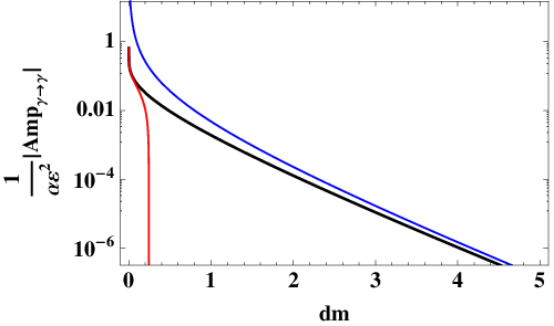
Let us now estimate the sensitivity of such an experiment. From Fig. 7 we can clearly see that the sensitivity will drop rapidly if . On the other hand for we find . Magnetic field strengths of the order can be reached in the laboratory. However, we have to stay below the critical field strength of the superconductor in order to prevent penetration of the superconductor by the magnetic field. In most materials, this ranges between and [20] although fields as high as T can be shielded in certain cases (cf., e.g. [21]). Modern magnetometers [22, 23, 24] can detect magnetic fields as low as ; therefore, using T seems relatively conservative. Accordingly we can expect a sensitivity in the to range77 7 It should be noted that the shielding of a magnetic field down to is certainly an experimental challenge. However, shielding on this level has been achieved [22].. The latter is in the ball park of the current best laboratory bounds [6, 17].
Finally, let us find out which mass scales for the minicharged particles we can probe in the experiment. Above we have already argued that we can only achieve good sensitivity as long as . On the other side we must have in order to suppress the ordinary leakage of magnetic fields through the superconducting shielding. Typical London penetration depths are of the order of (cf,. e.g., [25]). To avoid fields leaking directly through the shielding (without having to convert into hidden fields) at the level we need . The requirement then allows, in principle, to search for masses up to . With a shielding thicker than the minimal required size the experiment will be sensitive only to smaller masses.
5 Conclusions
In this note we have discussed a new type of tunneling process of particles through a barrier. Whereas ordinary quantum mechanical tunneling allows the particle to pass through a barrier of finite width and height, field theory with different particle species can allow particles to circumnavigate a barrier by converting into a real particle of a different species that does not interact with the barrier (cf. Fig. 1). As argued in this note, quantum field theory allows to circumnavigate the barrier by conversion into virtual particles that do not interact with the wall as depicted in Fig. 2. As an explicit example of this process we have calculated the tunneling probability via this “tunneling of the 3rd kind” for the case of photons coupled to minicharged particles.
From a formal perspective, this quantum field theoretic tunneling becomes reminiscent to quantum mechanical tunneling in the limit where a semiclassical approximation can be applied to the fluctuating propagators. Here, the tunneling probability follows a characteristic exponential behavior with an exponent that increases linearly with the wall thickness. By contrast, for high frequencies, our tunneling phenomenon has no quantum mechanical analogue anymore. Contrary to quantum mechanics where any finite barrier is eventually overcome in a classical sense for increasing energy, our (idealized) wall remains a potential barrier for all frequencies88 8 Of course, any real matter becomes translucent beyond a frequency scale typically set by the plasma frequency.. In particular, in the limit of small wall thickness, we observe a logarithmic increase of the tunneling probability. This dependence is characteristic for a quantum field theory phenomenon, as it probes the structure of vacuum polarization at high fluctuation momenta.
Experimentally, tunneling of the 3rd kind could be observed as a “light-shining-through-a-wall” signature. In contrast to the process in classical field theory where real particles traverse the wall, tunneling of the 3rd kind would lead to a strong dependence on the wall thickness.
Acknowledgements
The authors would like to thank Jens Braun for interesting discussions. HG acknowledges support by the DFG under contract Gi 328/5-1 (Heisenberg program) and by the DFG-SFB TR18.
Appendix A Photon transition amplitude using the Feynman-parameter representation of the polarization tensor
As a check of the derivation of the transition amplitude given in the main text we can use a different representation of the polarization tensor as given, e.g., in [26],
| (A.1) |
where the accounts for the small charge of the minicharged particles.
We now have to perform the partial Fourier transform of this expression according to Eq. (2.5) and insert it into Eq. (2.12). The details of this calculation depend on wether we are at small frequency regime or at large frequencies . We will now study these two cases separately.
A.1 Small-frequency limit
The first step in calculating the transition probability is to obtain the partial Fourier transform (2.5) of the polarization tensor given in (A.1) for ,
| (A.2) |
To perform this integration we continue into the complex plane and integrate along the contour shown in Fig. 8. The relevant parts of this contour are the two bits parallel to the imaginary axis. Together they contribute
| (A.3) |
We therefore need the imaginary part of . Using Eq. (A.1) one finds,
| (A.4) |
For , we can approximate the integral (A.3) by,
| (A.5) | |||||
The accuracy of this approximation is better than for . Inserting this expression into Eq. (2.12) we find,
| (A.6) | |||||
This agrees with the result found in Eq. (3.13).
A.2 High-frequency limit
The strategy for the high frequency limit is essentially the same as at low frequencies. However, the cut in the complex plane is somewhat more complicated as can be seen from Fig. 9. The essential difference to the low frequency case is that the branch cut extends to the real axis. Therefore, one has to properly take the poles of the propagators into account. The usual prescription for the propagators prescribe that the integration path is along the red line in Fig. 9. As can be seen from the figure, we have to close the integration contour along the black paths in order to avoid enclosing the cut inside the contour. In order to arrive at the red path, we then have to add the (finite) blue paths.
The essential contributions to the integral for the Fourier transform are then again the parts parallel to the imaginary axis and the blue paths,
| (A.7) | |||||
Extracting again the leading order behavior for large distances we find,
| (A.8) |
We note that for small masses the approximation is valid only at fairly large distances. Inserting this into Eq. (2.12), we obtain the transition probability,
| (A.9) |
References
- [1] F. Hund, Z. Phys., 43, 805 (1927); G. Gamow, Z. Phys. 51, 204 (1928).
- [2] G. Wentzel, Z. Phys. 38, 518 (1926); H.A. Kramers, Z. Phys. 39, 828 (1926); L. Brillouin, Comptes Rendus 183, 24 (1926).
- [3] P. Sikivie, Phys. Rev. Lett. 51 (1983) 1415 [Erratum-ibid. 52 (1984) 695]; A. A. Anselm, Yad. Fiz. 42 (1985) 1480; M. Gasperini, Phys. Rev. Lett. 59 (1987) 396; K. Van Bibber, N. R. Dagdeviren, S. E. Koonin, A. Kerman, and H. N. Nelson, Phys. Rev. Lett. 59, 759 (1987).
- [4] K. Ehret et al., arXiv:hep-ex/0702023; C. Robilliard,et al [BMV Collaboration], Phys. Rev. Lett. 99 (2007) 190403; A. S. Chou et al. [GammeV (T-969) Collaboration], Phys. Rev. Lett. 100 (2008) 080402; P. Pugnat et al. [OSQAR Collaboration], arXiv:0712.3362 [hep-ex]. M. Fouche et al. [BMV Collaboration], Phys. Rev. D 78 (2008) 032013; A. Afanasev et al. [LIPSS Collaboration], arXiv:0806.2631 [hep-ex].
- [5] L. B. Okun, Sov. Phys. JETP 56, 502 (1982).
- [6] M. Ahlers, H. Gies, J. Jaeckel, J. Redondo and A. Ringwald, Phys. Rev. D 76 (2007) 115005 [arXiv:0706.2836 [hep-ph]]; Phys. Rev. D 77 (2008) 095001 [arXiv:0711.4991 [hep-ph]].
- [7] H. Gies and R. Shaisultanov, Phys. Lett. B 480 (2000) 129 [arXiv:hep-ph/0009342].
- [8] B. Holdom, Phys. Lett. B 166 (1986) 196.
- [9] F. Brummer and J. Jaeckel, arXiv:0902.3615 [hep-ph].
- [10] K. R. Dienes, C. F. Kolda and J. March-Russell, Nucl. Phys. B 492 (1997) 104 [arXiv:hep-ph/9610479]; A. Lukas and K. S. Stelle, JHEP 0001 (2000) 010 [arXiv:hep-th/9911156]; D. Lust and S. Stieberger, arXiv:hep-th/0302221; S. A. Abel and B. W. Schofield, Nucl. Phys. B 685, 150 (2004) [hep-th/0311051]; S. Abel and J. Santiago, J. Phys. G 30, R83 (2004) [hep-ph/0404237]; R. Blumenhagen, G. Honecker and T. Weigand, JHEP 0506 (2005) 020 [arXiv:hep-th/0504232]; B. Batell and T. Gherghetta, Phys. Rev. D 73 (2006) 045016 [arXiv:hep-ph/0512356]; R. Blumenhagen, S. Moster and T. Weigand, Nucl. Phys. B 751 (2006) 186 [arXiv:hep-th/0603015]; S. A. Abel, J. Jaeckel, V. V. Khoze and A. Ringwald, Phys. Lett. B 666 (2008) 66 [arXiv:hep-ph/0608248]; S. A. Abel, M. D. Goodsell, J. Jaeckel, V. V. Khoze and A. Ringwald, JHEP 0807 (2008) 124 [arXiv:0803.1449 [hep-ph]].
- [11] J. Jaeckel and J. Redondo, Europhys. Lett. 84 (2008) 31002 [arXiv:0806.1115 [hep-ph]].
- [12] W. Dittrich and M. Reuter, Lect. Notes Phys. 220 (1985) 1.
- [13] for a review, see C. Schubert, Phys. Rept. 355, 73 (2001) [arXiv:hep-th/0101036].
- [14] I. K. Affleck, O. Alvarez and N. S. Manton, Nucl. Phys. B 197, 509 (1982).
- [15] S. P. Kim and D. N. Page, Phys. Rev. D 65, 105002 (2002) [arXiv:hep-th/0005078].
- [16] H. Gies and K. Klingmuller, Phys. Rev. D 72, 065001 (2005) [arXiv:hep-ph/0505099]; G. V. Dunne and C. Schubert, Phys. Rev. D 72, 105004 (2005) [arXiv:hep-th/0507174]; G. V. Dunne, Q. h. Wang, H. Gies and C. Schubert, Phys. Rev. D 73, 065028 (2006) [arXiv:hep-th/0602176]; R. Schutzhold, H. Gies and G. Dunne, Phys. Rev. Lett. 101, 130404 (2008) [arXiv:0807.0754 [hep-th]].
- [17] H. Gies, J. Jaeckel and A. Ringwald, Phys. Rev. Lett. 97 (2006) 140402 [arXiv:hep-ph/0607118]; A. Badertscher et al., Phys. Rev. D 75 (2007) 032004; M. Ahlers, H. Gies, J. Jaeckel and A. Ringwald, Phys. Rev. D 75 (2007) 035011 [arXiv:hep-ph/0612098]; S. N. Gninenko, N. V. Krasnikov and A. Rubbia, Phys. Rev. D 75 (2007) 075014 [hep-ph/0612203].
- [18] S. Davidson, S. Hannestad and G. Raffelt, JHEP 0005 (2000) 003 [arXiv:hep-ph/0001179].
- [19] E. Masso and J. Redondo, JCAP 0509 (2005) 015 [arXiv:hep-ph/0504202]; J. Jaeckel, E. Masso, J. Redondo, A. Ringwald and F. Takahashi, hep-ph/0605313; Phys. Rev. D 75 (2007) 013004 [arXiv:hep-ph/0610203]; E. Masso and J. Redondo, Phys. Rev. Lett. 97 (2006) 151802 [arXiv:hep-ph/0606163]; R. N. Mohapatra and S. Nasri, Phys. Rev. Lett. 98 (2007) 050402 [arXiv:hep-ph/0610068]; P. Brax, C. van de Bruck and A. C. Davis, Phys. Rev. Lett. 99 (2007) 121103 [arXiv:hep-ph/0703243].
- [20] J. W. Rohlf, “Modern physics from to ”, John Wiley & Sons, Inc, 1994.
- [21] T. Cavallin, R. Quarantiello, A. Matrone and G. Giunchi, J. Phys.: Conf. Ser. 43 (2006) 1015-1018.
- [22] J. C. Mester, J. M. Lockhart, B. Muhlfelder, D. O. Murray and M. A. Taber, Advances in Space Research, 25 (2000) 1185. See also http://einstein.stanford.edu/TECH/technology1.html.
- [23] D. Robbes, Sens. Actuators A: Phys. 129 (2006) 86.
- [24] J. C. Allred, R. N. Lyman, T. W. Kornack and M. V. Roamlis, Phys. Rev. Lett. 89 (2002) 130801.
- [25] Ch. Kittel, “Introduction to solid state physics”, John Wiley & Sons, Inc, 2005.
- [26] M. E. Peskin and D. V. Schroeder, “An Introduction To Quantum Field Theory,” Reading, USA: Addison-Wesley (1995) 842 p