Topologically distinct classes of valence bond solid states with their parent Hamiltonians

We begin with a quantum one-dimensional chain with $N$ lattice sites. In each site, the states $\left\{\left|m\right\rangle\right\}$ $(m=1,\ldots,d)$ transform under a $d$-dimensional irreducible representation (IR)$\ G_{d}$ of a Lie group $G$. Let us imagine that the physical Hilbert space is formed by two virtual identical particles, whose internal quantum numbers $\left\{\left|\alpha\right\rangle\right\}$ $(\alpha=1,\ldots,D)$ transform under the $D$-dimensional IR $G_{D}$ of the same Lie group $G$. Here we require that both singlet representation $G_{I}$ and IR $G_{d}$ are included in the tensor product decomposition of two $G_{D}$’s. The first requirement means that $G_{D}$ is a self-conjugate IR, i.e., the complex conjugate representation of $G_{D}$ is equivalent to $G_{D}$. The latter requirement can be implemented by the projection operator onto the physical Hilbert space [33]

where $P_{\alpha,\beta}^{[m]}$ is the Clebsch-Gordan coefficient defined by $P_{\alpha,\beta}^{[m]}=\langle G_{d},m|G_{D},\alpha;G_{D},\beta\rangle$. For VBS states in a periodic chain, each lattice site forms a valence-bond singlet $\left|I\right\rangle$ with its neighboring sites by pairing two virtual particles (See Fig. 1). Thus, the wave functions of the VBS states can be expressed as

where the valence-bond singlet $\left|I\right\rangle$ is given by

Here $Q_{\alpha,\beta}=\langle G_{I},I|G_{D},\alpha;G_{D},\beta\rangle$ is the Clebsch-Gordan coefficient of contracting two virtual $G_{D}$ representations to form a singlet representation $G_{I}$.

In the present formalism, the VBS states can be easily written in a matrix-product form. Since $P_{\alpha,\beta}^{[m]}$ and $Q_{\alpha,\beta}$ can be viewed as the matrix elements of $D\times D$ matrices of $P^{[m]}$ and $Q$, the VBS states in Eq. (2) can be thus written as the following matrix-product form:

where $A^{[m]}=P^{[m]}Q$ is a $D\times D$ matrix.

In periodic boundary conditions, the VBS states are invariant under lattice translation and transformation of the Lie group $G$ by construction. Although no local order parameters can be found to characterize these states, the $A^{[m]}$ matrices can fully determine their physical properties and render a “local” description. In open boundary conditions, edge states emerge at the two ends of the chain and then the matrix-product form of the VBS states is given by

where the matrix indices $\alpha,\beta$ denote the edge states. These edge degrees of freedom are described by two fractionalized particles transforming under $G_{D}$ representation of the Lie group $G$. Actually, the edge states and their representations are characteristic features of the VBS states, because they fully determine the local $A^{[m]}$ matrices.

Another useful way to represent the VBS states is to use boson or fermion realization methods. To illustrate this method, we trace back to the tensor product decomposition of IRs of Lie algebras. According to the group theory, the physical states $\left|m\right\rangle$ under the exchange of the two identical virtual particles is either symmetric or antisymmetric, depending on $G_{d}$ and $G_{D}$. Thus, the two virtual particles with fermion statistics create the antisymmetric states, while the bosonic particles yield the symmetric ones. In some cases, there are still several channels with the same exchange symmetry and additional projection has to be used to single out the physical states in $G_{d}$. For example, the fermionic realization of a spin-$2$ VBS state with virtual spin $J=3/2$ was considered in Ref. [34]. In this case, both site-quintet states ($S=2$) and site-singlet state ($S=0$) are allowed for two spin-$3/2$ fermions on a single site and an extra projection can remove the unphysical site-singlet state. There also exists the Schwinger boson realization which symmetrizes several fundamental IRs to form higher dimensional $G_{d}$’s. [11, 35, 36, 37] In fact, all these boson/fermion realization methods play the role of (sometimes partially) deleting the unphysical states.

Following the spirit of the AKLT model, one can construct the parent Hamiltonians such that the VBS states in Eq. (2) are their unique ground states. It is most convenient to work with the matrix-product form. For the matrix product states in Eq. (4), one can readily find that their reduced density matrix $\rho_{l}$ of $l$ successive sites has a rank of $D^{2}$ at most. This suggests that the reduced density matrix $\rho_{l}$ of these VBS states always have null space for sufficient large $l$. These states are annihilated by the local projection operators supported in the null space. Hence, they are always exact zero-energy ground states of the translationally invariant Hamiltonians

where $h_{i}$ contains a sum of the positive semi-definite projection operators supported in the null space from site $i$ to $i+l-1$. Previously, the parent Hamiltonians of the matrix product states for spin-ladder systems had been studied by similar methods.[38]

Let us begin with the simplest cases with only nearest-neighbor interactions. Now the null space can be obtained from the VBS picture of these states. The Hilbert space of two neighboring sites can be divided into a direct sum of different IR channels according to the tensor product decomposition $G_{d}\otimes G_{d}$. Once a valence-bond singlet of two virtual $G_{D}$’s is formed, the remaining two particles of adjacent sites can transform under a direct sum of IRs resulting from $G_{D}\otimes G_{D}$. Therefore, the IR channels contained in $G_{d}\otimes G_{d}$ but absent in $G_{D}\otimes G_{D}$ constitute the null space in the $2$-site reduced density matrix.

The above steps to locate the null space can be embedded in a matrix-product formalism. Practically, we rewrite the matrix-product states in Eq. (4) as

where the local matrix $g_{i}$ is defined by

To locate the null space, we resort to a “coarse-graining” procedure which converts the spins of adjacent sites to block spins. Since the VBS states are invariant under lattice translation, we can block the spins in sites $1$ and $2$ as

where the $D\times D$ matrices $B^{[G_{12},M_{12}^{G}]}$ are given by

Here $G_{12}$’s distinguish the IRs of nearest-neighbor bond spin channels and $\left|G_{12},M_{12}^{G}\right\rangle$ are the states in IR channel $G_{12}$. Correspondingly, $\langle G_{12},M_{12}^{G}|G_{d},m_{1};G_{d},m_{2}\rangle$ is the Clebsch-Gordan coefficient to combine the states of $G_{d}$’s into the states of $G_{12}$. In the example of $SU(2)$, $G_{12}$ denotes for the total bond spin $S_{12}$ and $-S_{12}\leq M_{12}^{S}\leq S_{12}$. After this “coarse-graining” procedure, the VBS states are transformed to a matrix-product form with $2$-site block spins, characterized by the block-independent matrices $B^{[G,M^{G}]}$. Since the $2$-site block spin states $\left|G_{12},M_{12}^{G}\right\rangle$ form a complete orthogonal set, the null space in the reduced density matrix of a $2$-site block is given by those IR channels with $B^{[G_{12},M_{12}^{G}]}=0$.

The null space for more than two adjacent sites is no longer easily visualized. However, the blocking process of $g$ matrices can be proceeded without any fundamental difficulties (See Fig. 2). In Sec. III B, we will study the spin-$1$ fermionic VBS state by using this powerful method.

The uniqueness of the VBS ground states of the constructed Hamiltonians has to be further clarified. Generally, the ground state degeneracy will occur if there exists another state with a larger null space in the reduced density matrix of the present interaction range. To lift the degeneracy, one can locate the null space in an extended range by blocking more spins and modify the Hamiltonian correspondingly. To justify the uniqueness, it is helpful to numerically diagonalize an open chain Hamiltonian with several lattice sites. If the numerically calculated ground-state degeneracy is $D^{2}$, i.e., the ground states are all contained in the matrix-product form, one can prove the uniqueness of VBS ground states by a mathematical induction method. The basic idea is to assume that the VBS states $\left|\Psi_{\alpha,\beta}\right\rangle$ in Eq. (5) are the only ground states of a projector Hamiltonian $H(N)$ of an open chain with $N$ sites. Then, the ground states of an open chain with $N+1$ lattice sites can be written as the following superposition of $\left|\Psi_{\alpha,\beta}\right\rangle$ and $\left|m_{N+1}\right\rangle$:

The vectors $\left|m_{N+1}\right\rangle$ on the site $N+1$ decouple from the excited states of $H(N)$ because such a coupling do not gain energy from the projector Hamiltonian $H(N+1)$. Now we can change the notation $W_{\beta\alpha,m_{N+1}}\equiv W_{\beta,\alpha}^{[m_{N+1}]}$ and then $\left|\Psi_{N+1}\right\rangle$ can be immediately written in a matrix-product form

where $D\times D$ matrix $W^{[m_{N+1}]}$ can be fully determined because $\left|\Psi_{N+1}\right\rangle$ are the zero-energy ground states of $H(N+1)$. After solving this eigenvalue problem, one can find that $\left|\Psi_{N+1}\right\rangle$ can be written in the form of Eq. (4). This final step completes the mathematical induction proof. For periodic boundary conditions, the VBS ground state should be a linear combination of the $D^{2}$ states in Eq. (5) and be annihilated by the extra projectors acting on the two ends of the chain. This will lead to the VBS ground state in the form of Eq. (4).

Actually, those matrix product states with $D^{2}$ linearly independent $\left|\Psi_{\alpha,\beta}\right\rangle$ in a finite open chain satisfy the so-called injective property. [21, 33, 39] The injectivity of the matrix product states not only ensures the ground-state uniqueness of the parent Hamiltonian, but also guarantees the existence of an energy gap and the exponentially decaying correlation functions of local operators.

As a warm up, let us apply the formalism in Sec. II to the spin-$S$ VBS states with two virtual spin-$J$ particles in each site. It is well-known that the product of two spin-$J$ representation

always contains a singlet and the physical spin-$S$ representation if $J\geq S/2$. After replacing the $SU(2)$ Clebsch-Gordan coefficient $P_{\alpha,\beta}^{[m]}=\langle S,m|J,\alpha;J,\beta\rangle$ in Eq. (1) and the spin-$J$ valence-bond singlet

in Eq. (3), the $(2J+1)\times(2J+1)$ matrix $A^{[m]}$ in Eq. (4) can be written as

where $-J\leq\alpha,\beta\leq J$. These $A^{[m]}$ matrices are rank $S$ irreducible spherical tensors and satisfy the following commutation relations:

where $J_{\pm}$ and $J_{z}$ generate the spin-$J$ representation of the $SU(2)$ algebra,

For the celebrated VBS states of the AKLT models, i.e., the case of virtual spin $J=S/2$, we can also use the Schwinger boson representation to express the VBS states. In the Schwinger boson language, the spin operators are expressed by

with a local constraint $a_{i}^{\dagger}a_{i}+b_{i}^{\dagger}b_{i}=2S$. Then, the integer spin-$S$ VBS states of the AKLT models in a periodic chain are expressed as [11]

where $\left|\mathrm{v}\right\rangle$ is the vacuum with no particle occupation. The matrix product form of these VBS states are obtained by Totsuka and Suzuki [23]. Since the null space of two neighboring sites is the total bond spin $S+1,\ldots,2S$ channels, the VBS states in Eq. (19) are exact ground states of AKLT Hamiltonians [10, 11]

where all $J_{S_{T}}>0$ and $P_{S_{T}}(i,j)$ is the projection operator on total bond spin channel $S_{T}$. These $SU(2)$ invariant projection operators can be written as polynomials of spin-exchange interactions $\mathbf{S}_{i}\cdot\mathbf{S}_{j}$ up to $2S$ powers

For $S/2<J<S$ cases, at first glance, the null space of two neighboring sites is given by the total bond spin channels $2J+1,\ldots,2S$, which is smaller than the VBS states of AKLT model. According to Sec. II B, one may conclude that next-nearest neighbor interactions are needed to be construct their parent Hamiltonians. However, there is an exception: the VBS states with $S=2$ and $J=3/2$. We will discuss this special case in Sec. III C.

Now we consider $S=1$ VBS state with virtual spin $J=1$, which belongs to the class in Sec. III A. Since $S=1$ is the only antisymmetric product of two virtual $J=1$ particles, one can use the fermionic statistics to implement the projection onto the physical $S=1$ subspace. Thus, the physical $S=1$ states are written as

The $SU(2)$ spin operators are $S_{i}^{a}=\sum_{\mu,\nu=1}^{3}c_{i\mu}^{{\dagger}}S_{\mu\nu}^{a}c_{i\nu}$ $(a=x,y,z)$, where $S^{a}$ are the usual $3\times 3$ spin-$1$ matrices. The total spin $\mathbf{S}_{i}^{2}=2$ on each site is imposed by a local constraint $\sum_{\mu=1}^{3}c_{i\mu}^{{\dagger}}c_{i\mu}=2$.

In terms of these fermionic variables, the $S=1$ VBS state with virtual spin $J=1$ can be exactly written as

which has a matrix product form in Eq. (4) with

Following the method in Sec. II B, we can construct the parent Hamiltonian for this fermionic VBS state. To locate the null space, it is sufficient to block three successive spins. The tensor decomposition of three spin-$1$ representation yields

which provides a natural basis for block spins. In this basis, the block states can be denoted by $\left|S_{12};S,M\right\rangle$, where $S$ and $M$ are total spin and magnetic quantum number of the three sites, $S_{12}$ is the total spin of the first two sites. For the representations $1^{\prime}$ and $2$, we have $S_{12}=1$. For the representations $1^{\prime\prime}$ and $2^{\prime}$, $S_{12}=2$. For the representations $0$ and $3$, the index $S_{12}$ can be suppressed and does not lead to misunderstanding.

After blocking the three spins, we obtain

where the $3\times 3$ matrices $C_{S_{12}}^{[S,M]}$ are given by

The matrices $C_{S_{12}}^{[S,M]}$ can be calculated by using Eq. (24). Firstly, we find that $C^{[0,0]}\neq 0$ and $C^{[3,M]}=0$. This means that the spin-$0$ singlet state is contained but the spin-$3$ states are absent in every three-site block. The other nonvanishing matrices $C_{S_{12}}^{[S,M]}$ satisfy the following equations:

According to Eq. (26), the unnormalized states contained in the $3$-site block $g_{1}g_{2}g_{3}$ are one spin-$0$ state, three spin-$1$ states

with $-1\leq M\leq 1$, and five spin-$2$ states

with $-2\leq M\leq 2$. By using the Gram-Schmidt orthogonalization method, we find that seven spin-$3$ states $\left|3,M\right\rangle$ with $-3\leq M\leq 3$, five spin-$2$ states

with $-2\leq M\leq 2$, six spin-$1$ states

with $-1\leq M\leq 1$ span the null space in the reduced density matrix of the $3$-site block. Therefore, the $3$-site projector Hamiltonian for which the spin-$1$ fermionic VBS state is the zero energy ground state is thus given by

where all $\lambda_{3},\lambda_{2},\lambda_{1},\lambda_{1}^{\prime}>0$.

It is interesting to compare the spin-$1$ fermionic VBS state with the spin-$1$ bosonic VBS state of AKLT model. In the fermionic VBS state, the two-point spin correlation function decays exponentially with a correlation length $\xi=1/\ln 2$, longer than that for the AKLT model ($\xi=1/\ln 3$). Besides the obvious difference of the edge spin representation in an open chain, we can also see a sharp difference by computing the non-local string order parameter [14, 23]

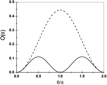
By using the transfer matrix method [22], we arrive at the result $\mathcal{O}(\theta)=\frac{1}{9}\sin^{2}\theta$ for the fermionic VBS state. For comparison, the values of the non-local order parameter $\mathcal{O}(\theta)$ for both the spin-$1$ fermionic VBS state and bosonic VBS state of the AKLT model are plotted in Fig. (3). For the spin-$1$ bosonic VBS state, $\mathcal{O}(\theta)$ reaches its maximum at $\theta=\pi$, which is reduced to the den Nijs-Rommelse string order parameter characterizing the hidden antiferromagnetic order in the AKLT VBS state. However, in the fermionic VBS state, $\mathcal{O}(\theta)$ has a minimum $\mathcal{O}(\pi)=0$ and the maximum value $1/9$ at both $\theta=\pi/2$ and $3\pi/2$. This signifies that the hidden antiferromagnetic picture totally breaks down in the $S=1$ fermionic VBS state. How to describe such a state has not been clear so far.

In Sec. III A, we have mentioned an exceptional example: $S=2$ VBS states with virtual spin $J=3/2$. Besides the absent bond total spin $S_{T}=4$ channel of neighboring sites, there is a new forbidden channel $S_{T}=2$ in this VBS state. [34] Therefore, its parent two-body Hamiltonian can be written as

with $J_{1},J_{2}>0$. According to Eq. (21), the projector Hamiltonian (30) can be rewritten as

In fact, the $S=2$ VBS state with virtual spin $J=3/2$ has a hidden $SO(5)$ symmetry and its matrix-product form was studied by Scalapino et al. [40] in an $SO(5)$ symmetric ladder system of interacting electrons.

The quantum spin-$2$ Hamiltonian in Eq. (30) belongs to a new class of exactly solvable quantum integer-spin chains introduced by the first three of us very recently. [34] The ground states of these Hamiltonians are $SO(2S+1)$ symmetric matrix-product states and exhibit hidden topological order. For $S=1$, the $SO(3)$ symmetric matrix product state becomes the VBS state of spin-$1$ AKLT model. For $S=2$, the $SO(5)$ symmetric matrix product state is the $S=2$ VBS state with virtual spin $J=3/2$. However, it was not clear whether this family of matrix product states has a valence-bond picture for $S\geq 3$. By using the framework in Sec. II, we will show that there is indeed a VBS picture for these matrix product states. Actually, the virtual particles in these VBS states transform under the $2^{S}$-dimensional spinor representation of $SO(2S+1)$.

It is convenient to promote the symmetry of the system and demand the spin-$S$ states on each site transform under the $(2S+1)$-dimensional vector representation of $SO(2S+1)$. The tensor product of two $SO(2S+1)$ vectors on the adjacent sites can be decomposed as

where the number above each underline is the dimension of the corresponding IR. These $SO(2S+1)$ IRs can be directly related to $SU(2)$ integer-spin IRs. Here $\underline{1}$ is the symmetric spin singlet, while the antisymmetric channel $\underline{S(2S+1)}$ and the symmetric channel $\underline{S(2S+3)}$ correspond to the total bond spin $S_{T}=1,3,\ldots,2S-1$ and $S_{T}=2,4,\ldots,2S$ states, respectively. Therefore, the $SO(2S+1)$ bond projection operators can be expressed using the spin projection operators as

On each lattice site, the $SO(2S+1)$ vectors can be formed by tensor decomposition of two virtual $2^{S}$-dimensional spinors

where $\binom{q}{2S+1}=\frac{(2S+1)!}{q!(2S-q+1)!}$. Note that $q=0$ and $q=1$ in Eq. (35) correspond to singlet representation and $(2S+1)$-dimensional vector representation, respectively. For $S=1$, Eq. (35) recovers the well-known decomposition $\underline{2}\otimes\underline{2}=\underline{1}\oplus\underline{3}$ of two spin-$1/2$ spinors. For $S=2$, Eq. (35) can be interpreted as the decomposition $\underline{4}\otimes\underline{4}=\underline{1}\oplus\underline{5}$ $\oplus\underline{10}$, where the $SO(5)$ spinors can be viewed as spin-$3/2$ variables because $SO(5)\simeq Sp(4)$. However, the $SO(2S+1)$ spinors in Eq. (35) for $S\geq 3$ do not have $SU(2)$ spin counterparts.

Following the discussions in Sec. II, the $SO(2S+1)$ symmetric VBS states can be constructed by combining the virtual spinors on the neighboring sites into valence-bond singlets. By comparing Eq. (32) and Eq. (35), one finds that the IR channel $\underline{S(2S+3)}$ for any two neighboring sites is absent in these VBS states. Here an interesting observation is that those IR channels with $q\geq 2$ in Eq. (35) are actually absent for two adjacent sites due to the projection of two virtual spinors onto the physical vector representation in each site. Therefore, the $SO(2S+1)$-invariant parent Hamiltonian for the $SO(2S+1)$ symmetric VBS states is given by

Since the null space of these VBS states is the non-zero even total spin channels, we can extend the $SO(2S+1)$-invariant parent Hamiltonian to the following $SU(2)$-invariant quantum integer-spin Hamiltonian

with all $J_{l}>0$.

Actually, the $SO(2S+1)$ symmetric VBS states are equivalent to the matrix product states studied in Ref. [34]. In the present VBS form, the origin of emergent $SO(2S+1)$ symmetry and the $2^{S}$ edge states on each boundary of an open chain are quite clear. Although the edge degrees of freedom in $S=1$ and $S=2$ cases can be viewed as $SU(2)$ spin variables, they transform under $SO(2S+1)$ spinor representation for $S\geq 3$ cases. It is interesting to compare these $SO(2S+1)$ symmetric VBS states to the spin-$S$ VBS states formed by virtual spin $J=(2^{S}-1)/2$ in Sec. III A. Although they are both unique in a periodic chain and $4^{S}$ fold degenerate in an open chain, their distinct edge states show that they belong to two different topological classes. These explicit examples imply that the ground state degeneracy is not sufficient to characterize the topological ordered states.

We begin with the $10$-dimensional $(2,0)$ adjoint representation of $SO(5)$. The bosonic $SO(5)/Sp(4)$ VBS state of this system was first considered by Schuricht and Rachel. [37] Their strategy is to construct the $(2,0)$ adjoint representation by two virtual particles transforming under the $(1,0)$ spinor representation,

where $(0,0)\$and $(1,1)$ are antisymmetric and $(2,0)$ is the only symmetric product representation. Therefore, one can obtain the physical $(2,0)$ adjoint representation by endowing bosonic statistics to the virtual $(1,0)$ spinor particles. This is analogous to the $SU(2)$ Schwinger boson representation which symmetrizes two spin-$1/2$ spinors to construct a spin-$1$ representation. Using the $4$-component $SO(5)$ Schwinger bosons, the $SO(5)$ generators in Eq. (38) can be defined by

where $\Gamma^{ab}=[\Gamma^{a},\Gamma^{b}]/2i$ and

For the $(2,0)$ adjoint representation with $\sum_{\mu=1}^{4}b_{\mu}^{{\dagger}}b_{\mu}=2$, the $10$ states in a bosonic language are shown in the $(2,0)$ weight diagram in Fig. 4. After a rotation by $45^{\circ}$, this weight diagram is identical to that given by Schuricht and Rachel. Here we choose the Clifford algebra generated by the $\Gamma$ matrices to define the $SO(5)$ generators. The advantage of our convention is to find an interesting non-local hidden string order in the $(2,0)$ bosonic VBS state below.

The $(2,0)$ bosonic $SO(5)$ VBS state is formed by contracting two $(1,0)$ spinors on neighboring sites into a valence-bond $SO(5)$ singlet. Its wave function can be written compactly as

where the antisymmetric matrix $R$ is given by

with the following properties: