Pointwise adaptive estimation
for robust and quantile regression
Abstract
A nonparametric procedure for robust regression estimation and for quantile regression is proposed which is completely data-driven and adapts locally to the regularity of the regression function. This is achieved by considering in each point M-estimators over different local neighbourhoods and by a local model selection procedure based on sequential testing. Non-asymptotic risk bounds are obtained, which yield rate-optimality for large sample asymptotics under weak conditions. Simulations for different univariate median regression models show good finite sample properties, also in comparison to traditional methods. The approach is extended to image denoising and applied to CT scans in cancer research.
2000 Mathematics Subject
Classification. Primary 62G08;
secondary 62G20, 62G35, 62F05, 62P10.
Keywords and Phrases. M-estimation, median regression, robust estimation, local model selection, unsupervised learning, local neighbourhood, median filter, Lepski procedure, minimax rate, image denoising, edge detection.
1 Introduction
We consider a generalized regression model
with i.i.d., in the design space and . The problems we have in view are those of robust nonparametric estimation of in the presence of heavy-tailed noise and of nonparametric quantile estimation, which is becoming more and more popular in applications. One main application will be robust image denoising. In the spirit of classical M-estimation [Huber] we therefore consider as the location parameter in the observation , that is
| (1.1) |
for some convex function with . We shall assume that is uniquely defined by (1.1), which is true in all cases of interest. If the have Lebesgue densities, then often an equivalent description is given by the first order condition where denotes the (weak) derivative. Standard examples are for the classical mean regression model (), for the median regression model () and the intermediate case for and for with some for the Huber estimator (). The quantile regression model is obtained for ( with quantile ), see e.g. ?. Since we shall care about robustness, we merely assume a mild moment condition for some and measure the error in -norm.
The function is not supposed to satisfy a global smoothness criterion, but we aim at estimating it locally in each point as efficiently as possible. The risk will then depend on local regularity properties, which we do not assume to be known. For spatially inhomogeneous functions, in the presence of jumps or for image denoising pointwise adaptive methods are much more appropriate than global smoothing methods. In classical mean regression local adaptivity can be achieved using wavelet thresholding or kernels with locally varying bandwidths, see ? for a discussion. In this ideal situation a data-driven choice among linear empirical quantities is performed. M-estimators are typically nonlinear and the standard approaches do not necessarily transfer directly. ?, for example, use an intermediate data binning and then apply wavelet thresholding to the binned data for median regression. On the other hand, ?, ? and ? consider kernels, smoothing splines and more general -estimation for quantile regression, but they all use global methods for choosing the tuning parameters like cross-validation or penalisation. Here, we develop a generic algorithm to select optimally among local M-estimators. In contrast to classical model selection, we do not only rely on the estimator values themselves to define a data-driven selection criterion. This has significant advantages in the present case of nonlinear base estimators.
Subsequently, we assume that the statistician has chosen the suitable definition of for the problem at hand and we use the corresponding sample versions to construct base estimators for the (generalized) regression function . In the spirit of classical nonparametrics, we assume that is locally almost constant around a given point . The statistical challenge is to select adaptively the right neighbourhood of where a local -estimator is applied. Let us write
| (1.2) |
for the location estimator on the set . If the minimizer is not unique, we just select one of them (e.g., a version of the sample median for even). Note that an extension to general local polynomial or more general local-likelihood estimation is straightforward, but this is not the focus of the present work. For each point let a family of nested neighbourhoods be given and set
Then the family forms the class of base estimators and we aim at selecting the best estimator of in this family.
1.1 Example.
Let the design space be with equidistant design points and take . Consider the symmetric windows generated by some bandwidths . Then is the classical median filter, see e.g. ? or ?.
Using Lepski’s approach as a starting point, we present our procedure to select optimally among local M-estimators in Section 2. We argue in a multiple testing interpretation that our procedure is usually more powerful. Moreover, it is equally simple to analyze and easy to implement. In Sections 3 and 4 we derive exact and asymptotic error bounds and the latter give optimal minimax rates for Hölder classes. The simulations in Section 5 show that our procedure has convincing finite sample properties. Moreover, they confirm that Lepski’s classical method applied to local median estimators suffers from oversmoothing because changes in the signal are not detected early enough due to the robustness of the median. Finally, the procedure has been implemented to denoise dynamical CT image sequences in Section 6, which is of key interest when assessing tumor therapies. Two more technical proofs are postponed to Section 7.
2 The procedure
2.1 Main ideas
As a starting point let us consider the standard ? method for selecting among , given the mean regression model with and . Note that the base estimators are then ordered according to decreasing variances: . On the other hand, the bias is usually increasing with increasing neighbourhoods . This is not always the case (for example, think of local means for a linear ), but true in particular for the worst case bias over smoothness classes like Hölder balls of functions. Lepski’s method can be understood as a multiple testing procedure where the hypothesis that is constant on is tested against the alternative of significant deviations. Always assuming that is true, we test sequentially whether is acceptable provided that the hypotheses have been accepted for all . Once the test of an is rejected, we select the base estimator corresponding to the last accepted hypothesis. The main point is thus to properly define the single significance tests for . Lepski’s method accepts if holds for all with suitable critical values . The wide applicability and success of Lepski’s method is also due to this very simple and intuitive test statistics.
In our nonlinear estimation case it turns out that tests for based on the differences of base estimators are often not optimal. To understand this fact, let us consider a toy model of two neighbourhoods with a piecewise constant median regression function equal to on and to on . The procedure therefore reduces to a simple two-sample location test between the observations in and in . We proceed by considering abstractly a two-sample location test where the first sample is i.i.d. with density and the second independent sample is i.i.d. with density . Our goal is to test for known . Given the Laplace distribution, we follow Lepski’s idea and put , the median over the first sample, and , the median over both samples. Then the test rejects if holds for appropriate . A more classical approach, though, relies on a likelihood ratio (LR) test or on a Wald-type test using the maximum likelihood estimator for . Since the LR test is not as simple, we focus on the Wald-test statistic which is given by the difference of the medians over the two samples. Hence, we reject if holds for appropriate . The following asymptotic result for the two test statistics is proved in Section 7.1.
2.1 Proposition.
Let be a symmetric and continuous density with and let , with be independently distributed. Then with denoting the cumulative distribution function of we obtain for
In particular, for we have and for we have the order , provided is Lipschitz continuous at zero.
Putting this result shows that under , i.e. , the test statistics and are asymptotically identically distributed, whereas has a larger asymptotic variance under any alternative than . In the above Laplace model with densities this deterioration is only negligible if the signal-to-noise ratio satisfies . This is exactly what we see in simulations, see e.g. Example 1 in Section 5 below. Since the Laplace model is Hellinger differentiable, the Wald-type test is (locally) asymptotically efficient for as is the LR test, see e.g. ?. Strictly speaking, when considering local alternatives for fixed and , i.e. , then the deterioration in using becomes also negligible. From a practical perspective, these local asymptotics are often not adequate, e.g. in image denoising, where we face relatively large signal differences at borders between objects and do not dispose of a very large number of observed pixels.
More generally, two-sample location tests can naturally be based on the difference of the in-sample location estimators. In consequence, we proceed differently in testing the hypotheses of homogeneity: When the hypotheses for have been accepted, we ask whether the observations in the new points are homogeneous with those in for . This means that our tests reject if the empirical location in the additional data
satisfies with certain critical values :
As in Lepski’s method, it is necessary to perform the testing for all and not only with to avoid that the signal slowly drifts away as the neighbourhoods grow. In most cases, though, will be rejected because the new piece is not in line with : due to the smaller variance of compared to , , this last test is the most powerful. It is then interesting to observe that for linear the test statistic is just a multiple of . Consequently, for mean regression with linear base estimators our method will not differ much from Lepski’s standard method, whereas the general nonlinear M-estimators are treated in a significantly different way, note also the numerical results in Section 5.
Observe that our approach breaks an ubiquitous paradigm in modern statistics and learning theory (see e.g. ? for model selection or ? for aggregation): we select the best base learner among in a data-driven way not only based on the estimator values themselves, but additionally on the statistics . Not only in the abstract modeling above, but also in implementations this idea turns out to be very advantageous for nonlinear estimators.
2.2 The algorithm
We want to select the best estimator among the family . Considering the law generated by the no-bias setting , we introduce the stochastic error levels
| (2.1) |
We apply the following sequential procedure for prescribed critical values and set :
- •
initialize ;
- •
repeat
if for allthen increase
else stop
until ; - •
put and .
This algorithm to determine can be cast in one formula:
3 Error analysis
3.1 Propagation and stopping late
We need a very natural property of the -estimator.
3.1 Assumption.
The location estimator in (1.2) satisfies for any set and any partition with pairwise disjoint sets :
3.2 Lemma.
If the function is strictly convex, then Assumption 3.1 is satisfied.
Proof.
Let us write as short-hand for , . Denoting by the right- and left-handed derivatives of the convex function , the functions , are strictly increasing with for all and
If were true for all , then
which contradicts the minimizing property of . Hence, holds and a symmetric argument shows . ∎
3.3 Remark.
If is not strictly convex, then we usually impose additional conditions to define uniquely. For any reasonable specific choice Assumption 3.1 should be satisfied. In particular, this is true for the sample median where we take for an even number of data points the mean of the order statistics.
3.4 Proposition.
Grant Assumption 3.1. Then we have for any
3.5 Remark.
This error propagation result is true ’-wise’, that is, it does not depend on the noise realisation. It is built into the construction of the selection procedure. An analogous result holds for Lepski’s original procedure [Lepski, Lepskietal].
3.6 Example.
For geometrically decreasing stochastic error levels in (2.1), in particular for the median filter from Example 1.1 with bandwidths , we have for , where means in the -notation. The late stopping error is of order , provided the critical values are non-increasing. This will imply that the error due to stopping later than some optimal is increased by at most the order of :
3.2 Critical values and stopping early
As the preceding analysis shows, small critical values lead to small errors caused by stopping late. On the other hand, the should not be too small in order to control the error of stopping early. To this end, we shall require a condition on the critical values in the no-bias situation under , that is for constant . In fact, we face a multiple testing problem, but with an estimation-type loss function. For some confidence parameter we select , , such that the condition
| (3.1) |
is satisfied. In order to obtain a unique prescription for each that equilibrates the errors for different stopping times of the algorithm, we can select the sequentially. We choose such that
and then each for given such that
| (3.2) |
To determine the in practice, we simulate in Monte Carlo iterations the pure noise case and calculate for each the error when the algorithm stops before the (theoretically optimal) index due to a rejected test involving . The critical values are determined such that this error is a fraction of the oracle estimation error . For this calibration step the original algorithm of Section 2.2 is taken, only modified by using instead of in the testing parts.
The selection rule for the critical values in Lepski’s procedure is the focus in the work by ?. Their idea is to transfer properties from the no-bias situation to the general nonparametric specification by bounding the likelihood between the two observation models. This approach, the so-called small modeling bias condition, could be applied here as well and will give similar results. On a practical level, the difference is that ? enlarge the moment from to in the calibration step, while we add the term to the testing values from the calibration. In the asymptotic analysis, however, the method by ? costs us some power in the logarithmic factor and we would thus not attain optimal rates over Hölder balls, cf. Section 4. Moreover, for robustness reasons, we do not want to require higher moment bounds for the error variables and the likelihood.
3.7 Definition.
Given the regression function , introduce its variation on
and consider the oracle-type index
This definition implies that for all the maximal bias of is less than its stochastic error level from (2.1) times the critical value . The next result, when specialised to , means intuitively that the error due to stopping before can be bounded in terms of the stochastic error of , involving the critical value as a factor. Let us also mention here that the rationale for the choice in the algorithm of Section 2.2 is to equilibrate maximal bias and stochastic error at step .
3.8 Proposition.
We have for any
Proof.
We shall write , etc. to indicate that , etc. depend on the underlying regression function . We shall need the inequality
| (3.3) |
which follows from
and by a symmetric argument for .
By definition of and using the condition on the as well as (3.3) for and , we obtain for all
The result follows from the isotonic decay of . ∎
3.3 Total risk bound
3.9 Theorem.
Assume that is non-increasing in . Then under Assumption 3.1 the following excess risk estimate holds for all :
Proof.
3.10 Example (continued).
For geometrically increasing bandwidths we obtain for and thus
The factor is the term we pay for adaptation.
4 Asymptotic risk
4.1 General result
We shall derive convergence rates for of the critical values . All quantities in the procedure may depend on , but we still write , and instead of , , . The notation will always mean with some independent of and is short for and . We work under the following assumption whose validity under mild conditions will be derived in the next subsection.
4.1 Assumption.
- (a)
The cardinalities of the neighbourhoods grow with geometric order:
for some fixed and with , as .
- (b)
For all sufficiently large we have
- (c)
For all with a moderate deviations bound applies: there is some such that
The following asymptotic bounds follow directly from the definitions:
Under Assumption 4.1 critical values of the same order as in the Gaussian case suffice.
4.3 Proposition.
Note that the chosen critical values are decreasing in , which has the desirable effect that we do not permit stopping at an early stage with the same probability as stopping at higher indices . Moreover, this guarantees that is non-increasing in , the hypothesis in Theorem 3.9. From Theorem 3.9 we therefore obtain the following asymptotic risk bound.
4.4 Corollary.
4.5 Example (continued).
Let us specify to -Hölder continuous , equidistant design and kernel estimators with geometrically increasing bandwidths , . Then we can choose and the index satisfies , that is and . This is the classical minimax rate for pointwise adaptive estimation in the one-dimensional -Hölder continuous case, see ? for the Gaussian case. Here, we have derived the same rate for pointwise adaptive -estimation under very weak conditions on the error distribution, compare the discussion on specific models below. Let us also mention that ? obtains the same rate result, but without logarithmic factor, for the non-adaptive median regression case.
Proof of Proposition 4.3.
Let . For sufficiently large Assumption 4.1(c) together with the asymptotics (using Assumption 4.1(a,b) and Lemma 4.2) yields
By Lemma 4.2 there is another constant such that for large
Our choice of with sufficiently large guarantees for large . We therefore more than satisfy (3.1) and the construction in (3.2) provided is sufficiently large:
For we obtain and thus . ∎
4.2 Specific models
The preceding asymptotic analysis was based on Assumption 4.1 where part (a) can be ensured by construction whereas parts (b) and (c) depend on the noise model and the choice of M-estimator. The most severe restriction will usually be the moderate deviation property of Assumption 4.1(c). In the case where the law of the error variable is absolutely continuous, this property holds by Corollary 2.1 in ? under the following conditions:
- (a)
for some and ;
- (b)
is Lebesgue-almost everywhere differentiable with derivative ;
- (c)
there are such that and are finite.
For mean regression we have and such that a finite exponential moment for is required. For median regression the result applies with and and because of no moment bound is required. The same is true for any robust statistic with bounded influence function, in particular for the Huber estimator and general quantile estimators. ? discusses that an exponential tail estimate for is also necessary to obtain a moderate deviation bound, which might be a serious drawback when using Lepski’s method with linear non-robust estimators.
For the median the requirements are not difficult to verify directly. Assumption 4.1(b) is for example established by ?, who show that for continuously differentiable around zero, , and :
Using a coupling result, we can establish Assumption 4.1(b,c) under even more general conditions, see Section 7.2 for a proof:
4.6 Proposition.
Assume that the have a Lebesgue density which is Lipschitz continuous at zero and satisfies , , . Noting , odd, we have
as well as for with
5 Simulation results

We illustrate our procedure by an implementation for median regression on and the estimation of the regression function at . We simulate equidistant observations with standardized errors (, ) that are (a) Laplace, (b) normal and (c) Student t-distributed with three degrees of freedom. The location is each time estimated by local sample means as well as by local sample medians. As neighbourhoods we take symmetric intervals around zero containing data points. This gives different base estimators.
The calibration of the procedure is performed for Laplace distributed errors with and . The variances , of the sample means are calculated exactly and those of the sample medians are approximated by their asymptotic values (which are quite close to Monte Carlo values). The critical values are chosen according to the prescription in (3.1). This is achieved in both cases, mean and median estimators, by using the choice in Proposition 4.3 with values that are calibrated by 10000 Monte Carlo runs for the pure noise situation. It turned out that this gives almost equally sized error contributions for the different values , as postulated in (3.2). The same calibration principle was applied for the original Lepski procedure with mean and median estimators.
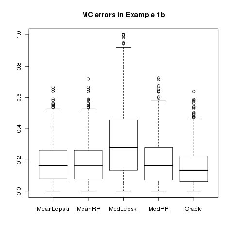
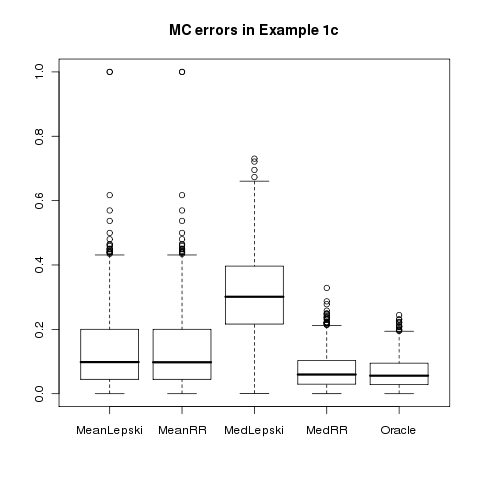
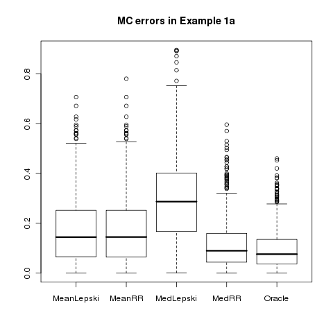
As a first example we take a simple change point problem by considering the regression function for and for , which can be considered as a toy model for edge detection in image restauration or for structural breaks in econometrics. In Figure 1 we show a typical data set in the Laplace case (a) together with box plots for the absolute error of the different methods in 1000 Monte Carlo repetitions: local means with Lepski’s and with our method, local medians with Lepski’s and with our method and the oracle method, which is just the sample median over . For exactly the same methods, especially still calibrated to Laplace errors, Figure 2 presents the results for Gaussian and heavy-tailed Student t(3) errors.
It is obvious that in all cases Lepski’s method applied to sample medians as base estimators works quite badly. This is due to the fact that this method stops far too late: the sample median over the complete intervals does not really ’notice’ the jump in the data. In fact, in the Laplace simulation study the oracle is selected by this method in less than of the cases while most often () the selection is which yields the times larger window . The methods using the sample mean estimators perform reasonably well and especially both very similarly. Still, they are clearly beaten by our median based procedure in cases (a) and (c) where the median is the more efficient location estimator. It is remarkable here that we nearly achieve the risk of the oracle median estimator. Even in the Gaussian case (b) the linear procedures have only minor advantages. Finally, we notice the robustness property that the calibration with the wrong error distribution in Figure 2 does not seriously affect the results.

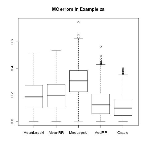
In a second example we consider the smooth regression function . Because we are estimating locally around , this is a caricature of a -function with and . Figure 3 shows again a typical data set and boxplots for the different methods in 1000 Monte Carlo runs under Laplace errors. This time the oracle choice is the window . Our median based procedure outperforms the others where the advantage over the mean-based approaches is again mainly due to the relative efficiency gain of size induced by the base estimators in the Laplace model. This gain, though, is not at all visible when using Lepski’s method for selecting among the sample medians. The results for the error distributions (b) and (c) resemble those of the first example, we confine ourselves to summarizing the numerical results for all examples in the following table, each time stating the Monte Carlo median of the absolute error:
| Ex. | Mean Lepski | Mean RR | Median Lepski | Median RR | Median Oracle |
|---|---|---|---|---|---|
| 1a | 0.1446 | 0.1450 | 0.2871 | 0.0897 | 0.0763 |
| 1b | 0.1640 | 0.1630 | 0.2795 | 0.1647 | 0.1325 |
| 1c | 0.0982 | 0.0978 | 0.3012 | 0.0596 | 0.0560 |
| 2a | 0.1846 | 0.1924 | 0.3051 | 0.1246 | 0.1005 |
| 2b | 0.1808 | 0.1886 | 0.3430 | 0.1586 | 0.1241 |
| 2c | 0.2102 | 0.2126 | 0.2455 | 0.1047 | 0.0822 |
Further simulation experiments confirm this picture. Especially for lower values of the moment our median-based procedure is very efficient, while sometimes for the mean-based procedures profit from less severe outliers in the Monte Carlo runs. In all these experiments the location is equally described by mean and median and we mainly see the efficiency gain of the sample median for non-Gaussian noise. For general quantile regression, however, linear methods do not apply and the standard Lepski procedures based on the nonlinear base estimators will perform badly. Our approach gives significantly better results. The error reductions by a factor of two and more, achieved in the median procedures above, confirm this very clearly.
6 Application


The proposed procedure is applied to denoise images used in the surveillance of cancer therapies. In Dynamic Contrast Enhanced Computer Tomography (DCE-CT) a contrast agent is injected in the human body and its diffusion over time is observed which is specific for different kinds of cell tissues and allows thus the surveillance of cancer therapies. For medical reasons the dose of contrast agent is kept small which leads to a poor signal-to-noise ratio. An analysis of residuals shows that the observational noise is well modeled by the Laplace distribution. Moreover, sometimes human movements produce significant outliers. Therefore local median estimation is employed. Especially for dynamical image sequences, the denoising is remarkably successful when the same spatial neighbourhoods are used over the whole observation period. This means that at each voxel location a vector-valued intensity function is observed under vector-valued noise . The vector encodes the intensity at time points recorded at spatial location . Our previously developed procedure perfectly applies to this situation, we just need a testing procedure between vector-valued local M-estimators.
Details of the experimental setup and the estimation procedure are discussed in ? and we merely give a rough description of the setting. A multiresolution test procedure is applied to compare different vector estimates. In a first pre-selection step for each voxel we disregard voxels that are significantly different from and construct then circular neighbourhoods around consisting only of non-rejected voxels. This allows geometrically richer neighborhood structures that in practice adapt well to the structure. Mathematically, the analysis of the algorithm remains the same when conditioning on the result of this first pre-selection.


For the present example we dispose of a DCE-CT sequence of recordings of -pixel images in the upper abdomen of a cancer patient. In Figure 4 the original image at time step 23 is depicted together with the result of our denoising procedure. The noise reduction is remarkable while fine structures like edges are well preserved and not smoothed out. The residuals in Figure 5(left) show some artefacts due to human body movements and CT radial artefacts, which our procedure removed as well. In Figure 5(right) a zoom into Figure 4(right) is shown together with the sequence of neighbourhoods constructed for one voxel inside the cancerogeneous tissue. The effect of the pre-selection step is clearly visible by the geometrically adaptive form of the neighbourhoods. Further results, in particular the denoised dynamics in certain voxels and an application to automatic clustering of cell tissues are reported in ?. The generality of our procedure has the potential to provide statistical solutions in many further applications where spatial inhomogeneity and robustness are key issues.
7 Appendix
7.1 Proof of Proposition 2.1
The asymptotic normality of the sample median is well known [vanderVaart, Corollary 21.5] and implies by independence the first asymptotic result.
Since the sample medians in the second case are not independent, we consider their joint distribution using empirical processes. Let us write for the cumulative distribution function of and denote by two independent standard Brownian bridges. Then empirical process theory yields by independence
The joint median satisfies in terms of the empirical distribution functions and of the two samples
Hence, it can be expressed as the functional of , assuming that the inverse is defined properly (e.g. giving the mean of all admissible values). Combining two-dimensional versions of Theorem 20.8 and Lemma 21.4 of ?, we infer
By symmetry of the right-hand side simplifies to
Consequently, is asymptotically normal with mean zero and variance
While for is straight-forward, we rewrite in terms of to study the behaviour as :
Because of by the Lipschitz property of , we obtain asymptotically
This gives . ∎
7.2 Proof of Proposition 4.6
We shall only consider the case of odd . Under the conditions of the proposition ? show the following result.
7.1 Theorem.
For all the sample can be realised on the same probability space as a standard normal random variable such that satisfies
where are constants depending on , but independent of .
The construction and the inequality of the theorem yield with some constant
On the other hand, because of we have for that the cdf satisfies and . From the formula for the density of
we therefore infer that for is finite and uniformly bounded. Hence, the Hölder inequality gives
which by Gaussian tail estimates is of order and thus for asymptotically negligible. This gives the upper moment bound for , the lower bound follows symmetrically. The -th moment is bounded by even simpler arguments.
The second assertion follows via quantile coupling from
∎
References
- [1] [] Arcones, M. A. (2002). Moderate Deviations for -estimators. Test 11(2), 465-500.
- [3] [] Arias-Castro, E. and D. Donoho (2006). Does median filtering truly preserve edges better than linear filtering?, Preprint in Math arXive math/0612422v1.
- [5] [] Brown, L. D., T. Cai and H. Zhou (2008). Robust nonparametric estimation via wavelet median regression. Annals of Statistics 36(5), 2055–2084.
- [7] [] Chu, J. T. and H. Hotelling (1955). The moments of the sample median. Annals of Math. Statistics 26(4), 593–606.
- [9] [] Hall, P. and M. C. Jones (1990). Adaptive -estimation in nonparametric regression. Annals of Statistics 18(4), 1712–1728.
- [11] [] Huber, P. J. (1964). Robust estimation of a location parameter. Annals of Mathematical Statistics 35(1), 73–101.
- [13] [] Katkovnik, V. and V. Spokoiny (2008). Spatially adaptive estimation via fitted local likelihood techniques. IEEE Transactions on Signal Processing 56(3), 873–886.
- [15] [] Koenker, R. (2005). Quantile Regression. Econometric Society Monographs 38, Cambridge University Press.
- [17] [] Lepskii, O. V. (1990). A problem of adaptive estimation in Gaussian white noise. Theory Probab. Appl. 35(3), 454–466. Translated from Teor. Veroyatnost. i Primenen. 35(3) (1990), 459–470.
- [19] [] Lepski, O., E. Mammen and V. Spokoiny (1997). Optimal spatial adaptation to inhomogeneous smoothness: an approach based on kernel estimates with variable bandwidth selectors. Annals of Statistics 25(3), 929–947.
- [21] [] Massart, P. (2005). Concentration inequalities and model selection. Ecole d’Eté de Probabilités de Saint-Flour XXXIII – 2003, Lecture Notes in Mathematics 1896, Springer, Berlin.
- [23] [] Polzehl, J. and V. Spokoiny (2003). Image denoising: pointwise adaptive approach. Annals of Statistics 31, 30–57.
- [25] [] Portnoy, S. (1997). Local asymptotics for quantile smoothing splines. Annals of Statistics 25(1), 414–434.
- [27] [] Rozenholc, Y., M. Reiß, D. Balvay and C.-A. Cuenod(2009). Growing time-homogeneous neighbourhoods for denoising and clustering dynamic contrast enhanced-CT sequences, Preprint Université Paris V.
- [29] [] Spokoiny, V. and C. Vial (2009). Parameter tuning in pointwise adaptation using a propagation approach, Annals of Statistics, to appear.
- [31] [] Truong, Y.K. (1989). Asymptotic Properties of Kernel Estimators Based on Local Medians, Annals of Statistics 17(2), 606–617.
- [33] [] Tsybakov, A. B. (2004). Optimal aggregation of classifiers in statistical learning. Annals of Statistics 32(1) 135–166.
- [35] [] van de Geer, S. (2003). Adaptive quantile regression, in Recent Trends in Nonparametric Statistics (Eds. M.G. Akritas and D.N. Politis), Elsevier Science, 235–250.
- [37] [] van der Vaart, A. (1998). Asymptotic Statistics, Cambridge University Press.