Effect of interactions on the diffusive expansion of a Bose-Einstein condensate in a 3D random potential

In this section we remind a few results concerning the averaged density profile $\bar{n}^{(0)}(\textbf{r},t)$ free of interactions in three dimensions. We assume that the condition of weak disorder $k_{\mu}\ell\gg 1$ [13] is fulfilled, where $k_{\mu}$ is the wavevector at energy $\mu$. As a consequence, the condensate expands mostly by diffusion in the random potential [9, 10]. This point will be discussed more deeply in section III.2. In the absence of interactions, the wave function of the condensate at time $t$ and position r is given by

where $\phi$ is the initial condensate wave function and $G_{\epsilon}$ is the Green’s function of Eq. (3). From here on, we consider large distances $r\gg\ell$ and long times $t\gg(\ell/v_{\mu})$, where $v_{\mu}=\hbar k_{\mu}/m$ is the velocity of a particle with kinetic energy $\mu$. The mean free time $\ell/v_{\mu}$ can be regarded as the time separating the ballistic regime $t\lesssim\ell/v_{\mu}$ from the multiple scattering one $t\gg\ell/v_{\mu}$ where atoms are scattered many times on the random potential. Under these assumptions we derive from Eq. (6) the following expression for $\overline{n}^{(0)}$ (more details can be found for example in Ref. [10]):

Here $\epsilon_{k}=\hbar^{2}k^{2}/2m$ and $P_{\epsilon}(\textbf{r},t)=\exp(-|\textbf{r}-\textbf{r}^{\prime}|^{2}/4D_{\epsilon}t)/(4\pi D_{\epsilon}t)^{3/2}$ is the diffusion propagator in three dimensions for a particle at energy $\epsilon$. $D_{\epsilon}=(1/3)\ell v_{\epsilon}$ is the diffusion coefficient of a particle of velocity $v_{\epsilon}=\sqrt{2\epsilon/m}$ [13]. The momentum distribution of the condensate $|\phi(\textbf{k})|^{2}\propto(1-k^{2}/2k_{\mu}^{2})H(1-k/\sqrt{2}k_{\mu})$, with $H(x)$ the Heaviside step function, is obtained from the following expansion scenario [5, 9, 10]: the BEC is generally produced in a harmonic trap potential of frequency $\omega$. The trap is turned off at some time, which causes the rapid expansion of the condensate, driven by strong interatomic interactions. At this initial stage of expansion we neglect the effect of disorder. After a time of the order of $1/\omega$, interactions become weak and the momentum distribution is given by $|\phi(\textbf{k})|^{2}$ [14]. We choose our initial time $t=0$ within this latter stage.

The calculation of the integral in Eq. (7) is straightforward and leads to:

where $f(x)$ can be expressed through special functions and $f(x)\simeq 0.04$ for $x\ll 1$. As pointed out in [10], the density profile is driven by a single parameter $D_{\mu}=(1/3)v_{\mu}\ell$, which can be regarded as the typical diffusion coefficient of the condensate. We plot the density profile in Fig. 1 as a function of time for three different distances $r$. $\bar{n}^{(0)}(\textbf{r},t)$ exhibits the well known decay in $t^{-3/2}$ in the long time limit $t\gg t_{\text{arrival}}$, where $t_{\text{arrival}}\sim r^{2}/D_{\mu}\sim(\ell/v_{\mu})(r/\ell)^{2}$ is the “arrival ”time at which the density reaches the maximum.

It must be noted that Eq. (8) describes a purely diffusive expansion and does not include the effects of Anderson localization. In Ref. [9], the authors found $\bar{n}^{(0)}\propto 1/t$ for $t>t_{\text{arrival}}$. A question then naturally arises: to which extent the diffusive result (8) is correct? In Ref. [9] the density profile has been studied for moderate values of $k_{\mu}\ell$, that is in the regime of strong disorder. When $k_{\mu}\ell$ is increased, the $1/t$ decay is expected to cross over to the $1/t^{3/2}$ decay typical for diffusion. To illustrate this cross-over we plot $\bar{n}^{(0)}(\textbf{r},t)$ including localization effects in Fig. 2 for three values of $k_{\mu}\ell$ and for $r=10\ell$ (three upper curves, orange, green and blue online). The lower curve in Fig. 2 (red online) is obtained from Eq. (8), i.e. by neglecting Anderson localization effects.

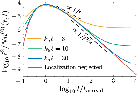
For $k_{\mu}\ell=3$, a significant fraction of atoms of the condensate are localized. At very short times, all diffusive atoms have already flown away and $\bar{n}^{(0)}\propto 1/t$, in agreement with Ref. [9]. For weak disorder ($k_{\mu}\ell=30inFig.\ref{n0_diffloc}$), the situation is very different: most atoms of the condensate propagate diffusively. Therefore the atomic density exhibits a $1/t^{3/2}$ decay characteristic for diffusion. Whatever $k_{\mu}\ell$ however, at very long times the atomic density saturates at a constant value $\bar{n}^{(0)}_{\text{loc}}\sim h(k_{\mu}\ell)(N/r^{3})(\ell/r)^{1/\nu}$, where $\nu$ is the critical exponent of the localization transition, and $h(k_{\mu}\ell)\propto 1/(k_{\mu}\ell)^{3}$ for $k_{\mu}\ell\gg 1$ and $h(k_{\mu}\ell)\propto\text{const}$ for $k_{\mu}\ell\ll 1$ [9]. We can estimate the time after which the diffusive approach breaks down by requiring that the saturation value $\bar{n}^{(0)}_{\text{loc}}$ is smaller than the limit $\bar{n}^{(0)}_{\text{dif}}\sim N/(D_{\mu}t)^{3/2}$ of Eq. (8) at long times $t\gg t_{\text{arrival}}$. This yields

as the maximum time at which diffusion model can be applied. When $k_{\mu}\ell\gg 1$ and $r\gg\ell$, $t_{\text{loc}}$ is always larger than $t_{\text{arrival}}$ and the diffusion model is hence valid in a broad time interval. To sum up, the condensate behaves diffusively ($\bar{n}^{(0)}\propto t^{-3/2}$) until $t=t_{\text{loc}}$, and beyond localization effects start to “freeze” the density profile at $n^{(0)}=\bar{n}^{(0)}_{\text{loc}}$. The conditions $k_{\mu}\ell\gg 1$ and $t\ll t_{\text{loc}}$ will be assumed throughout the remainder of the paper.

It should be noted that the mean free path $\ell$ is in principle modified in the presence of interactions. However in the following we will neglect the nonlinear corrections to $\ell$. This approximation is legitimate in the limit of long times, as we now show by making use of a criterion initially developed in [15] for monochromatic classical waves.

The mean free path is weakly affected by interactions provided that the scattering on the effective potential $g|\psi(\textbf{r},t)|^{2}$ is weak as compared to the scattering on the random potential. In other words, the mean free path $\ell^{(1)}$ associated with the interaction potential should be much larger than the mean free path $\ell^{(0)}=\ell$ associated with the random potential. $\ell^{(1)}$ can be evaluated from the short-range $``C_{1}"$ correlation function of the density $\overline{\delta n(\textbf{r},t)\delta n(\textbf{r}^{\prime},t)}$ which has been recently studied by Henseler and Shapiro [16]. We neglect here the contribution due to the long-range $``C_{2}"$ part of the density correlation function. This would be questionable for a condensate propagating in a quasi-one dimensional waveguide where $C_{2}$ was predicted to dominate at long times [17]. However the situation is different in an unbounded 3D random potential where we expect $C_{2}$ to decay with time. Indeed, let us consider a quasi-monochromatic wave pulse emitted from some point in an unbounded three-dimensional disordered medium. A straightforward calculation similar to that of Ref. [17] yields $C_{2}\propto(1/t^{2})/(k\ell)^{2}$ in the limit of long times. $C_{2}$ is therefore negligible with respect to $C_{1}$.

From [16] we write $\overline{\delta n(\textbf{r},t)\delta n(\textbf{r}^{\prime},t)}\simeq(2\pi\ell/k_{\mu}^{2})\bar{n}^{(0)}(\textbf{r},t)^{2}\delta{(\textbf{r}-\textbf{r}^{\prime})}$. For times $t\gg t_{\text{arrival}}$, this leads to $\ell^{(1)}\simeq(\hbar^{4}\pi/m^{2})(k_{\mu}^{2}/2\pi\ell)(D_{\mu}t)^{3}/(g^{2}N^{2})$. The condition $\ell^{(1)}\gg\ell$ then gives

where we introduced a dimensionless parameter $p=aN/\ell\sqrt{k_{\mu}\ell}$ that includes both interaction and disorder strengths. At this point, it is sufficient to keep in mind that in the weak disorder limit and under conditions of typical experiments, $p\ll 1$. For example with the data from Refs. [3] and [6] we find $p\sim 10^{-2}$. Therefore, the characteristic time $t_{1}$ is much smaller than $\ell/v_{\mu}$, such that the criterion (10) is automatically satisfied for long times $t\gg\ell/v_{\mu}$.

We now consider $\overline{\Delta n}(\textbf{r},t)$. From Eq. (4) we obtain

where $S(\textbf{r}^{\prime})$ is the right-hand side of Eq. (4) evaluated at $\textbf{r}^{\prime}$. Combining Eqs. (6) and (11) we obtain

where the six-point kernel $K$ is given by the connected part of a product of five Green’s functions, averaged over disorder:

The problem therefore reduces to finding the largest contribution to the kernel $K$ in the weak disorder limit $k_{\mu}\ell\gg 1$. This contribution is given by the diagram depicted in Fig. 3a. The diagram describes interaction of two matter waves at a point $\textbf{r}^{\prime}$. Diagrams of this type have been introduced some time ago for monochromatic classical waves in the context of nonlinear optics of disordered media [18]. In our case the situation is more general since $K$ contains a product of Green’s functions at five different energies.

Writing down explicitly the diagram of Fig. 3a, we obtain

where $\rho=mk_{\mu}/2\pi^{2}\hbar^{2}$ is the density of states at energy $\mu$ and $J=\int d^{3}\textbf{k}/(2\pi)^{3}\overline{G}(\textbf{k})\overline{G}^{*}(\textbf{k})=-i(\ell/v_{\mu})(4\pi^{3}\rho^{2}\ell/\hbar k_{\mu}^{2})$ is the diagram depicted in Fig. 3b. Now we introduce new variables $\Omega=\epsilon_{1}-\epsilon_{2}$, $\Omega^{\prime}=\epsilon_{3}-\epsilon_{4}$, $\epsilon=(\epsilon_{1}+\epsilon_{2})/2$, $\epsilon^{\prime}=(\epsilon_{3}+\epsilon_{4})/2$, and make use of results of Refs. [9, 16]:

where $P_{\epsilon}(\textbf{r},\Omega)=\exp(-|\textbf{r}|\sqrt{-i\Omega/\hbar D_{\epsilon}})/(4\pi D_{\epsilon}|\textbf{r}|)$ is the Fourier transform of the diffusion propagator at energy $\epsilon$. A similar relation holds for the integrals over $\textbf{r}_{1}$ and $\textbf{r}_{2}$. In the weak disorder limit $k_{\mu}\ell\gg 1$, $\text{Im}\overline{G}_{\epsilon^{\prime}}(\textbf{k}^{\prime})$ can be approximated by $-\pi\delta(\epsilon^{\prime}-\epsilon_{k^{\prime}})$ [10, 9, 16]. This finally leads to

The main difficulty of Eq. (16) lies in the four coupled integrals over energies and momenta, which make the exact calculation of $\overline{\Delta n}$ complicated. However, after some algebra and in the limit of long times, all integrals can be performed. The main lines of this calculation are reported in Appendix A. We find that for $t\gg t_{2}=(\ell/v_{\mu})(r/\ell)^{4}(k_{\mu}\ell)$, $\overline{\Delta n}$ becomes position independent as $\bar{n}^{(0)}$, and

It is quite remarkable that the first-order correction $\overline{\Delta n}$ has exactly the same time dependence as $\bar{n}^{(0)}$ at long times. Comparison of Eq. (17) to $\bar{n}_{\text{dif}}^{(0)}\simeq N/(D_{\mu}t)^{3/2}$ provides the criterion $p\ll 1$ as a condition of validity of our perturbative approach. As discussed in section IV.1, this criterion is usually satisfied in typical experiments, which validates the assumption of negligible interactions during expansion made in previous works [10, 16].

Few comments are in order. First, the negative sign in Eq. (17) indicates that repulsive interactions ($p>0$) tend to reinforce the diffusion process and the contrary for attractive interactions, which might have been expected. This appears more clearly if one writes the total density profile as

where we have defined an effective diffusion coefficient $D_{\text{eff}}=D_{\mu}/(1-p)^{2/3}$ taking interactions into account. For repulsive interactions for example, $p>0$ and therefore $D_{\text{eff}}>D_{\mu}$. Thus repulsive interactions seem to compete with localization, even though calculations of higher-order diagrams or a complete study of interactions within the localized regime would be necessary to confirm this effect. For extremely weak disorder ($k_{\mu}\ell\rightarrow\infty$) $p$ vanishes and $D_{\text{eff}}\simeq D_{\mu}$ whatever the interaction strength.

Another important remark is that the magnitude of the correction term (17) can be modified by increasing the strength of disorder independently of the strength of interactions, or vice versa. In particular, if we extrapolate our calculation to $k_{\mu}\ell\sim 1$, we find that even weak interactions may significantly affect the expansion of the condensate. In this case, the scattering length $a$ must be much less than $\ell/N$ to justify the neglect of interactions. This refines the condition of validity for the results of Ref. [9], where interactions were assumed weak, but no precise condition of weakness was given.

Our result (17) is only valid in the time interval $[t_{2},t_{\text{loc}}]$. For weak disorder, $t_{2}\ll t_{\text{loc}}$, which gives a broad range of validity to Eq. (17). For the sake of clarity we summarize all the time scales that we introduced above in Fig. 4.

References

- [1] For a review see L. Fallani, C. Fort, M. Inguscio. Adv. At. Mol. Opt. Phys. 56, 119 (2008).
- [2] L. Fallani, J. E. Lye, V. Guarrera, C. Fort and M. Inguscio, Phys. Rev. Lett. 98, 130404 (2007).
- [3] J.E. Lye et al., Phys. Rev. Lett. 95, 070401 (2005); D. Clement et al., ibid 95, 170409 (2005); C. Fort et al., ibid 95, 170410 (2005).
- [4] M. Modugno, Phys. Rev. A 73, 013606 (2006); E. Akkermans, S. Ghosh and Z. H. Musslimani, J. Phys. B: At. Mol. Opt. Phys. 41, 045302 (2008).
- [5] L. Sanchez-Palencia et al., Phys. Rev. Lett. 98, 210401 (2007).
- [6] J. Billy et al., Nature 453, 891 (2008).
- [7] G. Roati et al., Nature 453, 895 (2008).
- [8] P. W. Anderson, Phys. Rev. 109, 1492 (1958).
- [9] S.E. Skipetrov, A. Minguzzi, B.A. van Tiggelen, and B. Shapiro, Phys. Rev. Lett. 100, 165301 (2008).
- [10] B. Shapiro, Phys. Rev. Lett. 99, 060602 (2007).
- [11] L. Pitaevskii and S. Stringari, Bose-Einstein Condensation (Clarendon, Oxford, 2003).
- [12] A. S. Pikovsky and D. L. Shepelyansky, Phys. Rev. Lett. 100, 094101 (2008). S. Flach, D. O. Krimer, and Ch. Skokos, Phys. Rev. Lett. 102, 024101 (2009).
- [13] E. Akkermans and G. Montambaux, Mesoscopic Physics of Electrons and Photons (Cambridge University Press, Cambridge, 2007).
- [14] Yu. Kagan, E.L. Surkov, and G.V. Shlyapnikov, Phys. Rev. A 54, R1753 (1996); Y. Castin and R. Dum, Phys. Rev. Lett. 77, 5315 (1996).
- [15] B. Spivak and A. Zyuzin, Phys. Rev. Lett. 84, 1970 (2000).
- [16] P. Henseler and B. Shapiro, Phys. Rev. A 77, 033624 (2008).
- [17] N. Cherroret and S. E. Skipetrov, Phys. Rev. Lett. 101, 190406 (2008).
- [18] V. M. Agranovich and V. E. Kravtsov, Phys. Rev. B 43, 13691 (1991); A. Heiderich, R. Maynard and B. A. van Tiggelen, Opt. Commun. 115, 392 (1995); T. Wellens and B. Grémaud, J. Phys. B 39, 4719 (2006).
- [19] R.C. Kuhn et al., New. J. Phys. 9, 161 (2007).