Harmonic Gauge Perturbations of the Schwarzschild Metric
Abstract
\OnePageChapterThe satellite observatory LISA will be capable of detecting gravitational waves from extreme mass ratio inspirals (EMRIs), such as a small black hole orbiting a supermassive black hole. The gravitational effects of the much smaller mass can be treated as the perturbation of a known background metric, here the Schwarzschild metric. The perturbed Einstein field equations form a system of ten coupled partial differential equations. We solve the equations in the harmonic gauge, also called the Lorentz gauge or Lorenz gauge. Using separation of variables and Fourier transforms, we write the solutions in terms of six radial functions which satisfy decoupled ordinary differential equations. We then use the solutions to calculate the gravitational self-force for circular orbits. The self-force gives the first order perturbative corrections to the equations of motion.
Berndtson \otherdegreesB.A., University of Colorado, 1996 \degreeDoctor of Philosophy Ph.D., Physics \deptDepartment of Physics \advisorProf. Neil Ashby \readerDavid Bartlett \degreeyear2007 \dedication[Dedication]
To my family
Acknowledgements.
\OnePageChapterI thank my advisor, Neil Ashby, for his advice and patience, and the other committee members for their service. \LoFisShort\LoTisShortChapter 1 Introduction
The satellite observatory LISA will be capable of detecting gravitational waves from extreme mass ratio inspirals (EMRIs). These occur when a compact star, such as a black hole, neutron star, or white dwarf, is captured by a supermassive black hole [80]. The evolution of EMRI orbits and their gravitational waveforms can be calculated using black hole perturbation theory. An introduction to black hole perturbation theory, including the harmonic gauge, is in section 1.1. An outline of the remainder of the thesis is in section 1.2.
1.1 Black Hole Perturbation Theory
The Schwarzschild metric is
| (1.1) |
where the standard coordinates have been used. It is a solution of the Einstein field equations, which are
| (1.2) |
The Schwarzschild metric is a vacuum solution, meaning . In (1.2), the gravitational constant and speed of light are shown explicitly. Generally though, we will use geometrized units, for which . We will use this and other notational conventions as described by Misner, Thorne and Wheeler [71], including the metric signature of (1.1) and form of the field equations (1.2).
Black hole perturbation theory for the Schwarzschild metric was formulated by Regge and Wheeler [98] and extended by Zerilli [115]. A summary of their method follows, which is taken mainly from their articles. A small perturbation is added to the background Schwarzschild metric . Our physical problem involves a small mass orbiting a much larger black hole , so is proportional to the mass ratio . Accordingly, the total perturbed metric is
| (1.3) |
The inverse perturbed metric is
| (1.4) |
The perturbed field equations are linear in :
| (1.5) |
The semicolons represent covariant differentiation with respect to the background metric . For the Schwarzschild metric, the Ricci tensor and Ricci scalar are zero, so the field equations simplify to
| (1.6) |
As discussed in [71], the left side of the perturbed equations represents the propagation of a wave interacting with the background spacetime curvature. The stress energy tensor is the covariant form of
| (1.7) |
where the delta function represents a point mass or test particle. The stress energy tensor divergence equation is
| (1.8) |
which, when applied to (1.7), gives the background geodesic equations of motion [32].
Regge, Wheeler and Zerilli solved the perturbed field equations using separation of variables. The angular dependence is contained in tensor harmonics, which are obtained from the familiar spherical harmonics. A Fourier transform separates the time dependence, leaving a set of radial ordinary differential equations to be solved. The solution was simplified by making a particular choice of gauge, the so-called Regge-Wheeler gauge. A gauge is a choice of coordinates. A change of gauge is a small change of coordinates
| (1.9) |
which causes the metric perturbation to change as
| (1.10) |
Here, “small” means . Although the perturbation is gauge dependent, the perturbed field equations in (1.6) are gauge invariant [32].
We will use the notation of Ashby [4], which is different from, and simpler than, Zerilli’s notation [115]. Because the background metric is spherically symmetric, the perturbation can be split into odd and even parity parts. This decomposition gives
| (1.11) |
The odd parity terms are
| (1.12) |
where
| (1.13) |
| (1.14) |
The even parity part is
| (1.15) |
Asterisks represent symmetric components. The angular functions are the tensor harmonics. The Regge-Wheeler gauge is defined by setting four radial factors equal to zero: the odd parity and the even parity , and . The trace of the metric perturbation is
| (1.16) |
where
| (1.17) |
Similarly, the stress energy tensor may be decomposed in terms of tensor harmonics and Fourier transforms. The covariant components are
| (1.18) |
where
| (1.19) |
and
| (1.20) |
The trace of the stress energy tensor is
| (1.21) |
and its multipole decomposition is
| (1.22) |
where
| (1.23) |
The gauge change vector is
| (1.24) |
where is the Kronecker delta and where
| (1.25) |
| (1.26) |
Because a gauge change is a small change of coordinates, the quantities and are of order , just as the perturbation is. The remaining two terms in (1.24) are also order and are discussed in subsections 3.2.4 and 2.2.2, respectively.
Regge and Wheeler showed that the odd parity components could be expressed in terms of a single radial scalar function, the Regge-Wheeler function, which satisfies a second order ordinary differential equation. Zerilli did the same for the even parity components; his function is called the Zerilli function. Later, Moncrief showed that these two functions are gauge invariant [72].
The Regge-Wheeler gauge is comparatively simple, but we will work in a different gauge, the harmonic gauge. The reason for this choice is that the equations for the gravitational self-force were derived in the harmonic gauge [70], [96]. The basic harmonic gauge field equations are given in [71], which uses the term Lorentz gauge. The spelling Lorenz is also used in the literature [86]. We first define the trace-reversed metric
| (1.27) |
where the trace is
| (1.28) |
The harmonic gauge is defined by the condition
| (1.29) |
Using (1.27) and (1.29), the field equations (1.6) simplify to
| (1.30) |
| (1.31) |
which are the terms eliminated in going from (1.6) to (1.30). The harmonic gauge condition (1.29) and field equations (1.30) are preserved after a gauge change which satisfies
| (1.32) |
The harmonic gauge equations above apply when the background metric describes a curved spacetime, as the Schwarzschild metric does.
Before discussing further the harmonic gauge for the Schwarzschild metric, it is helpful to review a much simpler example, the plane wave. The analysis below of the plane wave is taken from Weinberg’s chapter on gravitational radiation [110], supplemented by [104]. The plane wave is a perturbation of the flat space metric . The perturbed metric is
| (1.33) |
We can choose the gauge so that
| (1.34) |
In this gauge, the homogeneous field equations are
| (1.35) |
where is the flat spacetime D’Alembertian operator. The gauge (1.34) and field equations (1.35) are preserved by gauge changes which satisfy
| (1.36) |
Equations (1.34)-(1.36) are the flat spacetime background metric equivalents of the curved background spacetime equations (1.29)-(1.30), (1.32). Moreover, we can derive equations (1.34)-(1.36) from the curved spacetime expressions, although Weinberg derives his equations ab initio.
Weinberg shows that the solution to the field equations (1.35) is a wave
| (1.37) |
where is the symmetric polarization tensor. Here and elsewhere in this thesis, an overbar usually represents complex conjugation; however, this notational rule does not apply to (1.27) and its trace, . Substituting (1.37) into the field equations (1.35) and gauge definition (1.34) yields
| (1.38) |
respectively. A symmetric matrix has at most ten independent components. The gauge definition (1.34) represents four constraints, which reduce the number of independent components, or polarizations, to six. The gauge transformation vector appropriate to (1.37) is
| (1.39) |
where is a constant vector (equation (9.14) of [104]). A change of gauge modifies the polarization tensors as
| (1.40) |
The solution (1.37) is a plane wave traveling in the positive -direction if the wave vector is
| (1.41) |
For such a plane wave, the six independent polarizations can be written as the following linear combinations of :
| (1.42) |
The remaining components are not independent and depend on the six above, by symmetry and by the following equations:
| (1.43) |
Weinberg shows the components are gauge invariant, because they can not be removed by a coordinate transformation. However, , and can be eliminated by a coordinate transformation which satisfies (1.36) and preserves the gauge condition (1.34).
The six independent components (1.42) behave differently when a rotation is made about the -axis, the direction of wave propagation. Specifically, Weinberg shows
| (1.44) |
where the primes denote polarizations after rotation through an angle . A plane wave has helicity if
| (1.45) |
The rotation results (1.44) show that the gravitational plane wave (1.37) can be decomposed into six pieces: two of helicity , two of helicity and two of helicity . The trace of the polarization tensor is , so the zero helicity pieces are related to the trace of . Only the helicity components are physically meaningful, because they alone can not be removed by a coordinate transformation.
Schwarzschild metric perturbation theory has an analogue to the different helicity functions of the plane wave example. The generalized Regge-Wheeler equation is
| (1.46) |
where the potential is
| (1.47) |
The generalized Regge-Wheeler equation is discussed in [55], [63], [64]. It represents a wave interacting with an effective potential that results from the background spacetime curvature. The parameter is the spin or spin weight, and it corresponds to the different helicities of the plane wave example. The case is equal to the Regge-Wheeler function that was derived in the Regge-Wheeler gauge. Described in [98] and [115], the coordinate is
| (1.48) |
so that
| (1.49) |
and
| (1.50) |
Because , we have . Due to this relation, is called the “tortoise” coordinate [71]. Throughout this thesis, the parameter is defined as [115]
| (1.51) |
which implies
| (1.52) |
The generalized Regge-Wheeler equation will often be abbreviated as
| (1.53) |
where the operator is defined by the left side of (1.46). The source is constructed from the radial coefficients of the stress energy tensor (1.18)-(1.20).
The solutions for the harmonic gauge are described in terms of generalized Regge-Wheeler functions. Specifically, the odd parity solutions are written in terms of two generalized Regge-Wheeler functions, one with and the other with . The even parity solutions are written in terms of two functions with , one with and one with . The even parity spin function is actually the Zerilli function, but can be related to the spin Regge-Wheeler function by differential operators. The even and odd parity spin functions are gauge invariant. These six functions correspond to the six different helicity states of the plane wave example.
1.2 Summary of Thesis
Most of this thesis discusses the solution of the field equations in the harmonic gauge (1.30). Chapters 2 and 3 summarize the derivation of the odd and even parity solutions, respectively. The solutions are expressions for the radial coefficients (such as and ) of the angular functions in the odd (1.12) and even (1.15) parity metric perturbations . The cases of non-zero and zero angular frequency are handled separately. Both inhomogeneous and homogeneous solutions are covered. Some of the even parity solutions are listed separately in the appendices. With a few cited exceptions, the solutions derived in these two chapters are new and constitute the main research results of this thesis.
Chapter 4 covers the equations of motion. Both the background geodesic and gravitational self-force equations are presented. Chapter 5 discusses the stress energy tensor for a point mass, its multipole decomposition and its Fourier transforms for circular and elliptic orbits. The chapter includes formulae for the radial coefficients (such as and ) of the angular functions of the stress energy components in equations (1.19) and (1.20). Chapter 6 has homogeneous and inhomogeneous solutions for the generalized Regge-Wheeler and Zerilli equations. Chapter 7 explains how to use the harmonic gauge solutions to calculate gravitational waveforms and energy and angular momentum fluxes. Chapter 8 contains results of numerical calculations, mainly of the gravitational self-force for circular orbits. Chapter 9 is a brief conclusion.
Mathematica was used extensively for the derivations. Some results are attributed to unpublished work of Neil Ashby, which is cited as reference [4]. Among other things, he rederived and corrected the published solutions for the Regge-Wheeler gauge. He also provided Mathematica tools for simplifying expressions (including derivatives of angular functions) and for deriving recursion relations for infinite series. Quantities related to the background Schwarzschild metric, such as Christoffel symbols and Riemann curvature tensor components, were calculated with Mathematica-based software written by him.
Chapter 2 Odd Parity Solutions
This chapter contains the derivation of the odd parity field equations and their solutions in the harmonic gauge. We will use separation of variables to reduce the perturbed field equations to a system of three coupled ordinary differential equations, with independent variable . The resulting equations are solved in terms of generalized Regge-Wheeler functions, with and . Section 2.1 describes the non-zero frequency solutions, with the cases of spherical harmonic index and handled separately. Section 2.2 does the same for zero frequency. Section 2.3 concludes with a discussion of homogeneous solutions.
2.1 Non-Zero Frequency Solutions
Subsection 2.1.1 covers the case . Subsection 2.1.2 shows how the solutions for can be obtained from the solutions for .
2.1.1 Solutions for
The first step is to derive the radial field equations, using separation of variables. The method of derivation is similar to that used by Regge, Wheeler and Zerilli for the Regge-Wheeler gauge [98], [115]. We substitute the odd parity metric perturbations from (1.11)-(1.12) and stress energy tensor components from (1.18)-(1.19) into the harmonic gauge field equations (1.30), which are a system of coupled partial differential equations. Because the equations are Fourier transforms, the time dependence is in the exponentials , which divide off. Partial derivatives with respect to time become factors of angular frequency, using the rule . The angular variables and are contained entirely in the tensor harmonics and their derivatives. After simplifying the angular derivatives, the tensor harmonics also separate off, and we are left with the following radial factors to the odd parity field equations:
| (2.1) |
| (2.2) |
| (2.3) |
Primes signify differentiation with respect to . Generally, functional dependence on and will be suppressed, so that, for example, abbreviates and represents . However, the system of equations (2.1)-(2.3) must be solved for each combination of indices , and . Equation (2.1) comes from the component of the field equations (multiplied by a factor of ). Similarly, (2.2) and (2.3) are obtained from the and components, respectively. Because there are only three odd parity radial functions (, and ), there are only three odd parity radial field equations. The remaining odd parity components of the field equations are either zero or have the same radial factors as (2.1)-(2.3).
Each of the three radial field equations can be written in the form
| (2.4) |
or, alternatively,
| (2.5) |
where the “other terms” are at most first order derivatives. The inverse Fourier transform of (2.5) is
| (2.6) |
which is a wave equation. In the time domain, the field equations are a hyperbolic system of partial differential equations. The system is a well-posed initial value problem and can be solved numerically in the time domain [7], [70]. The field equations above agree with those derived by Barack and Lousto [7], who used different notation and worked in the time domain.
Related equations are also separable. The harmonic gauge condition leads to the radial equation
| (2.7) |
The stress energy tensor divergence equation, , is [4]
| (2.8) |
For a change of gauge described by equations (1.10) and (1.24)-(1.25), the radial perturbation factors transform as
| (2.9) |
| (2.10) |
| (2.11) |
where the function is order [4], [98], [115]. To preserve the harmonic gauge, a change of gauge must satisfy , and the associated radial equation is
| (2.12) |
This is the homogeneous generalized Regge-Wheeler equation, with . Odd parity gauge changes which preserve the harmonic gauge are implemented by adding homogeneous spin 1 solutions to the metric perturbations.
To derive another first order equation, differentiate (2.7) with respect to and use (2.2) and (2.7) to eliminate and . This gives
| (2.13) |
Unlike the harmonic gauge condition (2.7), which applies only in the harmonic gauge, equation (2.13) is gauge invariant and applies in any gauge. As shown by (2.9)-(2.11), the radial functions are gauge dependent; however, a gauge change to one (say ) is canceled by changes to the remaining functions, leaving equation (2.13) the same in the new gauge. The stress energy tensor term is coordinate dependent; however, it is order , so any changes to it are order . Thus, (2.13) is gauge invariant to linear order in . In contrast, a gauge change applied to (2.7) results in additional terms involving and its derivatives, unless the change satisfies (2.12) and preserves the harmonic gauge. Equation (2.7) is invariant only under changes which preserve the harmonic gauge, but equation (2.13) is invariant under arbitrary gauge changes. Another way of deriving (2.13) is to substitute the odd parity metric perturbations into (1.6), the general perturbation field equations applicable to any gauge. Equation (2.13) is obtained from the component, multiplied by . Because (1.6) is gauge invariant, so is (2.13).
Regge and Wheeler showed that, in the Regge-Wheeler gauge, the odd parity perturbations can be written in terms of a single scalar function which satisfies a wave equation called the Regge-Wheeler equation [98]. In the notation of this thesis, this function is the odd parity , and the Regge-Wheeler equation is
| (2.14) |
Equation (2.14) is the generalized Regge-Wheeler equation from (1.46), with . Subsequently, Moncrief proved that the Regge-Wheeler function is gauge invariant [72]-[73]. He deduced a formula for in terms of the metric perturbations. Adjusting for differences in notation between his paper and this thesis, his expression is
| (2.15) |
Although the radial perturbation functions are gauge dependent, is gauge invariant. Moncrief showed that any gauge change in would be offset by changes to and , as follows. From equation (2.10), the term containing changes by . Using (2.11), the terms with and change by . The changes cancel each other, leaving invariant. Moncrief did not derive his result in the harmonic gauge, but his work can be used here, because (2.15) is gauge invariant.
In equation (2.14), the quantity is a source term constructed from the radial components of the stress energy tensor. To find , substitute (2.15) into the Regge-Wheeler equation and simplify with the other harmonic gauge equations, obtaining
| (2.16) |
Taking into account differences in notation, equation (2.16) agrees with Zerilli’s result in the Regge-Wheeler gauge [115], as corrected by others [4], [102].
Solutions for and can be written terms of and . By solving (2.15) for , we find
| (2.17) |
We then use (2.17) and its radial derivative to eliminate and from (2.7) and solve for to get
| (2.18) |
Substituting for in the field equation (2.3), we have
| (2.19) |
where the operator was defined in (1.53). The left side is the generalized Regge-Wheeler equation, with . To complete the odd parity solutions, we will solve (2.19) for and substitute the result into (2.18) and (2.17).
The form of (2.19) suggests the following trial solution
| (2.20) |
where is a constant and the other quantities are functions of . To find the unknowns, we insert into the left side of (2.19) and obtain
| (2.21) |
The “source terms” are complicated expressions involving , and , and their first and second radial derivatives. The “ terms” are terms proportional to either or . In order that does not couple to , we set the coefficients of and equal to zero, which produces two second order differential equations for and . The coefficient of gives
| (2.22) |
and the coefficient of yields
| (2.23) |
Equations (2.22) and (2.23) can be solved by substituting series trial solutions, namely,
| (2.24) |
Doing so leads to
| (2.25) |
and
| (2.26) |
The series terminate if
| (2.27) |
which gives
| (2.28) |
These solutions can be verified by substitution into (2.22) and (2.23). If we choose , we have
| (2.29) |
As mentioned previously, the “source terms” in equation (2.21) include second radial derivatives of , and . The second derivatives are eliminated if and
| (2.30) |
Substituting these results into , we finally obtain the solution to equation (2.19),
| (2.31) |
and its radial derivative,
| (2.32) |
Equation (2.15) defines in terms of odd parity radial functions. An analogous expression for is derived by solving (2.31) for and using (2.18) and (2.17) to eliminate and , respectively. The result is
| (2.33) |
Substituting (2.33) into the spin generalized Regge-Wheeler equation gives the differential equation for ,
| (2.34) |
Equation (2.8) may be used to eliminate . Although (2.15) is gauge invariant, equation (2.33) is not: it is valid only in the harmonic gauge. If a gauge change is made which satisfies (2.12) and thereby preserves the harmonic gauge, changes by a homogeneous spin solution (in other words, a homogeneous solution of (2.34)). Stated differently,
| (2.35) |
where refers to the homogeneous solution. Even though has changed by , the right side of (2.35) has the same form as (2.33). In this limited sense, the formula for in (2.33) is invariant under gauge changes which preserve the harmonic gauge. Nevertheless, the behavior of is different from that of , because after any change of gauge.
The above solutions for and are substituted into (2.18) and (2.17) to obtain
| (2.36) |
and
| (2.37) |
and their radial derivatives,
| (2.38) |
and
| (2.39) |
One may verify by substitution that these solutions satisfy the field equations, as well as the harmonic gauge condition, the first order equation (2.13), and the definitions of and .
The solutions also can be checked by transforming from the harmonic gauge (“H”) to the Regge-Wheeler gauge (“RW”). By definition, . Applying equation (2.11), we set and substitute into equations (2.9) and (2.10) to obtain
| (2.40) |
and
| (2.41) |
Adjusting for differences in notation, the Regge-Wheeler gauge solutions agree with those obtained by Zerilli and others [4], [102], [115]. Equation (2.41) can be solved for to give the Regge-Wheeler expression for . In the limit , Moncrief’s formula, equation (2.15), reduces to theirs.
The preceding paragraph suggests another way of deriving the harmonic gauge solutions. Instead of working throughout in the harmonic gauge, we could have started in the Regge-Wheeler gauge (where the solutions are known) and looked for the gauge transformation vector that would take us from the Regge-Wheeler gauge to the harmonic gauge. To do so, we would need to derive the radial function in (1.25) that we would then substitute into (2.9)-(2.11), with the superscript “old” referring to the Regge-Wheeler gauge and “new” being the harmonic gauge. This approach was begun in [102], where a differential equation for the gauge transformation vector was derived. The equation is similar to (2.19) above, although the derivation in [102] is very different. However, the authors of [102] did not solve their gauge transformation equation (they put it aside for “future study”) and did not complete the derivation of the harmonic gauge solutions.
Because equation (2.13) is gauge invariant, the formula for in (2.15) is not unique. We can solve (2.13) for and substitute for in (2.15). The result is
| (2.42) |
where
| (2.43) |
The superscript “JT” stands for Jhingan and Tanaka, who derived in the Regge-Wheeler gauge using a different method and notation and showed that it is gauge invariant [61]. We will use the superscript “JT” because they discuss this form extensively, even though they acknowledge it was derived earlier by others. In (2.43), the factor of indicates that is the time derivative of , and Jhingan and Tanaka constructed so that it would be the Fourier transform of a time integral of . Applying equations (2.9) and (2.10), a gauge change in is canceled by corresponding gauge changes to and , leaving invariant. After substituting into the Regge-Wheeler equation and simplifying, we obtain a source term given by
| (2.44) |
Adjusting for differences in notation, the source term agrees with that in [61]. Using (2.42), the field equation solutions can be rewritten in terms of , if desired.
This completes the derivation of the odd parity non-zero frequency solutions, for . We started with the harmonic gauge field equations given by (1.30), which are partial differential equations. Using separation of variables, that system was reduced to the three radial field equations in (2.1)-(2.3), a system of coupled ordinary differential equations. The solutions to the radial equations are written in terms of and , each of which satisfies its own decoupled second order differential equation. To calculate , and , we would first solve the decoupled equations for and and then substitute the results into the solutions (2.36), (2.37) and (2.31). In this manner, we have simplified the problem from a system of coupled partial differential equations to two decoupled ordinary differential equations.
2.1.2 Solutions for
Although subsection 2.1.1 assumed that , most of the results derived there can be used for . One difference is that is no longer present. In equation (1.12) for the odd parity metric perturbations, the angular functions and are zero [115], so does not exist for . Similarly, is non-existent. Further, there are only two field equations, (2.1) and (2.2), because (2.3) is the radial coefficient of or . To show that and are zero, substitute the spherical harmonics for [3] into the definitions of (1.13) and (1.14).
2.2 Zero Frequency Solutions
The zero-frequency equations and solutions have . Factors of are due to time derivatives of the factor . Because this exponential contains the time dependence of the metric perturbation, solutions with are time independent solutions. Below, the cases and are discussed separately.
2.2.1 Solutions for
We can use the field and related equations from subsection 2.1.1, after substituting . However, no longer couples to and through the radial field equations. Instead, has a separate field equation, (2.1), while and solve a coupled system, (2.2) and (2.3). This decoupling of also appears in other equations, namely, the harmonic gauge condition (2.7) and the gauge invariant first order equation (2.13). Neither contains if . Further, the source for (2.1), , no longer couples to and through the stress energy tensor divergence equation (2.8).
We will solve for and first. Using (2.13) to eliminate from (2.3), we have
| (2.45) |
This is the generalized Regge-Wheeler equation, with . Accordingly,
| (2.46) |
where
| (2.47) |
Here, is different from in subsection 2.1.1, even though the same notation is used for both functions. Substituting (2.46) into (2.13) gives
| (2.48) |
and the radial derivative is
| (2.49) |
By substitution, the reader may verify that (2.46) and (2.48) are solutions to the zero frequency field and related equations that involve and . The two solutions depend on , but not . This means the definition of in (2.15) is not valid for zero frequency, as that definition is in terms of and .
The next step is to solve the remaining field equation, (2.1), for . From (2.9), is gauge invariant when , and the solution will be in terms of the spin Regge-Wheeler function, which is also gauge invariant. Using (2.43), we set , so that
| (2.50) |
and
| (2.51) |
After differentiating (2.50) and using (2.1) to eliminate , we find that
| (2.52) |
Equations (2.50) and (2.52) can be solved for and , giving
| (2.53) |
and
| (2.54) |
For zero frequency and , the metric perturbation can be written in terms of spin and spin generalized Regge-Wheeler functions, just as for non-zero frequency modes.
2.2.2 Solutions for
For , the function is not present, as explained in subsection 2.1.2. From (2.1) and (2.2), the field equations become
| (2.55) |
| (2.56) |
The harmonic gauge condition simplifies to
| (2.57) |
For the non-zero frequency mode having , we used the solutions for , but we can not do that here. The zero frequency solutions for have factors of , but if .
The rules for a change of gauge are somewhat different from (2.9)-(2.10) and are discussed in [108]. Rewritten in terms of instead of , the rules become
| (2.58) |
| (2.59) |
where the replacement has been used in (2.9). The symbol is short for . Referring to (1.24)-(1.25), the odd parity gauge change vector for is
| (2.60) |
The rules are modified in order to allow a gauge change of the form
| (2.61) |
where is a constant. Although written in terms of , this is actually a change in the coordinate [108]. The modification is necessary in order to allow a gauge change in . If we substitute (2.61) into (2.58) and (2.59), then changes by , but is unaltered [108]. Because is only linear in , remains time independent. This form of gauge change could not have been used for other modes. For non-zero frequency modes, the gauge vector time dependence is in the factor . For zero frequency modes with , the new form would cause to grow linearly with time, as (2.11) shows. As a result, the zero frequency is effectively gauge invariant for (by (2.9)), but gauge dependent for .
From (2.12), a gauge change which preserves the harmonic gauge must be a solution of
| (2.62) |
which is the generalized Regge-Wheeler equation with , written in the time domain. The most general zero frequency gauge change which satisfies (2.62) and leaves the perturbation time independent is
| (2.63) |
If were non-linear in , or had some other time dependence, and would be time dependent. The first term of (2.63) changes only ; the second, only . The last term, , changes neither nor , so we will disregard it.
For , the zero and non-zero frequency gauge changes rules may be combined to give
| (2.64) |
This satisfies (2.62), provided that is a solution of (2.12) with . For non-zero frequency, is the function referred to in section 2.1. For zero frequency, is equal to the last two terms of (2.63).
We will solve the field equations first for and then for . If we use (2.57) and its radial derivative to eliminate and then from (2.56), we find that the left side of (2.56) is reduced to zero. This means . More directly, the same result can be obtained from (2.13), by substituting and . Because , the function is a homogeneous solution of (2.56) and (2.57). Accordingly,
| (2.65) |
where is a constant. If C is non-zero, we can nevertheless zero out by a gauge transformation described in (2.63), with and . Because is entirely gauge dependent, we can set in (2.65), so for and .
The other radial function, , represents the orbital angular momentum of the small mass [115]. Equation (2.55) has homogeneous solutions of and . From them, we can construct an inhomogeneous solution using variation of parameters [67], or a Green’s function [60]. Either method produces
| (2.66) |
| (2.67) |
where is short for . Alternatively, the solution for may be written in terms of a spin Regge-Wheeler function and its radial derivative; however, the resulting expressions are more complicated than those given above. The limits and are generic and should be replaced by limits appropriate to the orbital motion. For example, an elliptic orbit would have limits of (periastron) instead of and (apastron) instead of .
We can analytically evaluate the integrals in (2.66) for a circular orbit of radius , with the stress energy tensor expressions in Chapter 5. Doing so gives
| (2.68) |
where we have used [3]
| (2.69) |
The factor is the orbital angular momentum per unit mass (4.10), (4.26). To find the perturbation, we substitute (2.68) and into (1.12), getting
| (2.70) |
The other perturbation components are zero for this mode, and the superscript “10” is short for . The solution (2.70) was also calculated by Detweiler and Poisson [34], following Zerilli [115]. They note the solution for resembles the linearized Kerr metric. Specifically, the term has the same form as the component of the Kerr metric linearized to , with taking the place of the Kerr angular momentum parameter . In contrast, the solution for differs from the background metric only by a gauge transformation [34]. As discussed in [115] and [34], the solution for this multipole represents the orbital angular momentum of the mass and the change in angular momentum that occurs at the orbital radius.
2.3 Homogeneous Solutions
This section discusses homogeneous solutions of the odd parity field equations. We will start with the non-zero frequency case, with .
The radial field equations in (2.1)-(2.3) form a system of three second order linear ordinary differential equations. From the theory of differential equations, such a system may be reformulated as an equivalent system of six first order equations, and the new system will have at most six linearly independent homogeneous solutions [117]. Accordingly, one might expect that the field equations could also have six homogeneous solutions. However, consider the following system of four first order homogeneous linear differential equations:
| (2.71) |
| (2.72) |
| (2.73) |
| (2.74) |
Equation (2.72) is the homogeneous form of (2.3), rewritten in terms of (2.71). Similarly, (2.73) is the harmonic gauge condition, (2.7), and (2.74) is from (2.13). Thus, the system of four is derived from the field equations and the harmonic gauge condition. Moreover, it is possible to show that the homogeneous form of the field equations can be derived from (2.71)-(2.74). Each system implies the other, so the system of four and the homogeneous field equations are equivalent. The system of four has only four linearly independent solutions. Because these four equations are equivalent to the homogeneous form of the field equations, the odd parity field equations also have only four linearly independent homogeneous solutions. This reduction from six to four evidently occurs because of the harmonic gauge condition, which is a differentiable constraint.
Solutions to a system of linear differential equations are written in the form of column vectors. If a matrix formed from the solution vectors has a non-zero determinant, the solutions are linearly independent [117].
We need to find four linearly independent solution vectors for the system (2.71)-(2.74). As explained in Chapter 6, the non-zero frequency generalized Regge-Wheeler equation has two linearly independent homogeneous solutions: , which represents an ingoing wave near the event horizon, and , which represents an outgoing wave at large . This suggests that we form one solution vector from each of , , and . The first solution vector is
| (2.75) |
The is for transpose, because is a column vector, rather than the row vector displayed above. The first component of (2.75) comes from the term of (2.36), the second component from the terms of (2.37), the third from (2.31) and the fourth from (2.32). The second solution, , is obtained from by replacing with . The third vector is
| (2.76) |
where
| (2.77) |
| (2.78) |
The fourth solution, , is obtained from by replacing with . The function
| (2.79) |
is the determinant of the matrix whose four columns are through . In equation (2.79), the factors and are the Wronskians (6.6) of the generalized Regge-Wheeler homogeneous solutions. Because the determinant (2.79) is non-zero, the solution vectors through are linearly independent. From the theory of ordinary differential equations, any homogeneous solution to the system (2.71)-(2.74) (and, by extension, the field equations (2.1)-(2.3)) can be written as a linear combination of the solution vectors described above. Accordingly, homogeneous solutions of the odd parity field equations are formed from combinations of the generalized Regge-Wheeler functions and . This result is to be expected, given the form of the inhomogeneous solutions derived in subsection 2.1.1.
Gauge transformations which preserve the harmonic gauge are implemented by adding homogeneous spin solutions (2.12). Because of this gauge freedom, the contributions to the homogeneous solutions above can be removed by a gauge transformation which preserves the harmonic gauge. However, the solutions can not be so removed. This is because the spin Regge-Wheeler functions are gauge invariant. To modify the two solution vectors attributable to (, ), we would have to transform to a different gauge, such as the Regge-Wheeler gauge. Also, a harmonic gauge preserving change adds only homogeneous solutions, so it can not remove the inhomogeneous contributions derived in subsection 2.1.1.
The homogeneous solutions above assumed . For , the radial functions and are not present, as explained in subsection 2.1.2. We are left with a two equation system that is composed of (2.73)-(2.74), modified by the substitution . Using similar arguments to the case, we can show that the homogeneous solutions can be written solely in terms of and . Specifically, the solution vectors are the first two components of and . Moreover, these homogeneous solutions can be removed by a gauge transformation which preserves the harmonic gauge.
The homogeneous solutions above are for non-zero frequency. For zero frequency and , we use the following first order system instead:
| (2.80) |
| (2.81) |
| (2.82) |
| (2.83) |
We use these four first order equations because of the decoupling of the zero frequency from and . If we had wished, we could have used the non-zero frequency equivalents of (2.80)-(2.83) instead of (2.71)-(2.74) in our discussion of the non-zero frequency case. Equation (2.81) is the homogeneous form of the field equation (2.1), rewritten in terms of (2.80). Equation (2.82) is the zero frequency harmonic gauge condition (2.7), and equation (2.83) is the zero frequency form of (2.13). It is possible to show that the system (2.80)-(2.83) is equivalent to the zero frequency field equations, in the same way that (2.71)-(2.74) are equivalent to the non-zero frequency field equations. Accordingly, the zero frequency field equations have only four linearly independent homogeneous solutions.
As discussed in Chapter 6, there are two linearly independent zero frequency homogeneous solutions of the generalized Regge-Wheeler equation. One solution, , is finite as , but diverges like as . The other solution, , is bounded for large , but diverges logarithmically near the event horizon. With arguments similar to the non-zero frequency case, we can show that all zero frequency homogeneous solutions can be written as combinations of , , and . Further, the and solutions can be removed by means of a gauge transformation which preserves the harmonic gauge. Although the spin solutions remain, they are divergent, either at the horizon or for large . To prevent an unphysical divergence, we set them equal to zero by choice of integration constants. A similar conclusion was reached by Vishveshwara [108], although he did not work in the harmonic gauge.
For , is no longer present, and the homogeneous solution for is zero, as discussed in subsection 2.2.2. This leaves the single second order differential equation for , which is written as two first order equations in (2.80)-(2.81). For reference, the second order equation is (2.55)
| (2.84) |
which has homogeneous solutions of the form
| (2.85) |
The solution can be removed by means of a transformation which preserves the harmonic gauge and does not change . To do so, simply set and in the gauge change vector (2.63). However, the solution can not be so removed by (2.63). Moreover, if we try to remove this solution by means of a gauge transformation which does not preserve the harmonic gauge, then will grow linearly with time, based on (2.58)-(2.59). In other words, the solution is not a purely gauge perturbation. It will be zero only if we set on physical grounds.
Homogeneous solutions of (2.84) were studied by Vishveshwara [108], who did not work in the harmonic gauge specifically. He showed that the solution gives
| (2.86) |
which he observed is a rotational perturbation. Vishveshwara further demonstrated that this solution can be made regular near the event horizon and elsewhere in Kruskal coordinates, following a gauge transformation which is equivalent to adding a specific solution described in [108].
The rotational perturbation mentioned by Vishveshwara would describe the slow rotation of the central mass . Because we are assuming that the central mass is not rotating, we set in (2.85). Orbital angular momentum of the small mass is described by the inhomogeneous perturbation (2.66), not by a homogeneous solution.
The work above shows that the physically meaningful odd parity homogeneous solutions to the harmonic gauge field equations are constructed from the non-zero frequency , which is gauge invariant. Other possible homogeneous solutions either can be removed by means of a gauge transformation which preserves the harmonic gauge, or do not satisfy the applicable boundary conditions.
Chapter 3 Even Parity Solutions
Although more complicated, the calculation of the even parity solutions is similar to the odd parity derivation. First, the field and related equations are obtained using separation of variables. Next, the seven radial field equations are solved in terms of solutions to decoupled equations. The spin 2 Regge-Wheeler function is replaced by a related spin 2 function, the solution to Zerilli’s equation. There are three generalized Regge-Wheeler functions: one with and two with . Non-zero frequency solutions are in section 3.1, zero frequency solutions are in section 3.2, homogeneous solutions are in section 3.3, and an interim summary of results is in section 3.4.
3.1 Non-Zero Frequency Solutions
Subsection 3.1.1 describes solutions for . Subsection 3.1.2 explains how the solutions for and can be derived from the solutions.
3.1.1 Solutions for
Using separation of variables, we derive the seven radial field equations:
| (3.1) |
| (3.2) |
| (3.3) |
| (3.4) |
| (3.5) |
| (3.6) |
| (3.7) |
Equations (3.1), (3.2) and (3.3) are formed by combining the , and components of (1.30) so that each equation contains the second derivative of only one radial function. The and components of the even parity metric perturbation in (1.15) each has two angular functions, and . This structure carries over to the field equations, and the component used above is the coefficient of the term. The remaining four field equations come from the , , and components, respectively, and here the component is the coefficient of the term. Other components of (1.30) duplicate the equations listed above. As is the case for odd parity, the even parity field equations form a hyperbolic system of partial differential equations when written in the time domain. Taking into account differences in notation, the field equations agree with those in [7].
The harmonic gauge condition (1.29) gives three radial equations,
| (3.8) |
| (3.9) |
| (3.10) |
Equations (3.8) and (3.9) are from the and components of (1.29), respectively, while (3.10) can be obtained from either the or component.
The stress energy tensor divergence equation (1.8) also generates three radial equations,
| (3.11) |
| (3.12) |
| (3.13) |
Equations (3.11), (3.12) and (3.13) are from the , and (or ) components of (1.8), respectively.
Applying (1.10), a gauge change alters the radial perturbation functions by
| (3.14) |
| (3.15) |
| (3.16) |
| (3.17) |
| (3.18) |
| (3.19) |
| (3.20) |
where , and are defined in (1.26) [4], [98], [115]. From (1.32), a gauge transformation that preserves the harmonic gauge must satisfy a system of three coupled differential equations,
| (3.21) |
| (3.22) |
| (3.23) |
Equations (3.21), (3.22) and (3.23) are from the , and (or ) components of (1.32), respectively. Later, we will show that solutions to this system can be written in terms of homogeneous solutions of the generalized Regge-Wheeler equation, with or .
By differentiating the harmonic gauge conditions in (3.8)-(3.10), we can eliminate second derivatives from the field equations to get four additional first order equations,
| (3.24) |
| (3.25) |
| (3.26) |
| (3.27) |
Alternatively, these four equations may be derived by manipulating the radial equations which can be extracted from (1.31), after using the field equations to eliminate second derivatives with respect to . Three of the equations, (3.24), (3.25) and (3.26), are gauge invariant to linear order, just as odd parity equation (2.13) is. The three also can be obtained from the gauge invariant general perturbation field equations in (1.6). In the Regge-Wheeler gauge, equation (3.26) simplifies to the so-called “algebraic relation” used by Regge, Wheeler and Zerilli to solve the field equations in their gauge [98], [115].
The first step in solving the field equations is to derive an even parity gauge invariant function, as was done for the odd parity case. To do so, we write a trial solution in the form
| (3.28) |
and then use (3.14)-(3.20) to find a combination of the radial functions which leaves invariant. One combination, which will be called , is
| (3.29) |
A gauge change in one radial function, say , is canceled by changes in the remaining radial functions. In the Regge-Wheeler gauge, we have . With these substitutions,
| (3.30) |
where the superscript “RW” signifies that and are computed in the Regge-Wheeler gauge. Zerilli derived expressions for and [115], which have been corrected by others [4], [102]. The corrected expressions can be solved for [4], and the resulting “Zerilli form” agrees with (3.30). Solutions in the Regge-Wheeler gauge are provided below, in equations (3.86)-(3.89).
The odd parity gauge invariant function, , is a solution of the generalized Regge-Wheeler equation, with . The even parity is the solution of a related equation, the Zerilli equation [115], which is
| (3.31) |
As will be shown in Chapter 6, homogeneous solutions of the Zerilli equation can be written in terms of homogeneous solutions of the Regge-Wheeler equation, using differential operators. This means the Zerilli function is also a spin function, which justifies using the notation for it as well. In fact, Jhingan and Tanaka showed that, in the Regge-Wheeler gauge, the even parity metric perturbation can be written in terms of Regge-Wheeler rather than Zerilli functions, although it is somewhat more complicated to do so [61]. Presumably, the same could be done for other gauges.
The source term, , in (3.31) is calculated by substituting into the Zerilli equation and simplifying with the field and related equations. The result is
| (3.32) |
Using (3.11), we can eliminate and rewrite the source as
| (3.33) |
Although (3.32) and (3.33) are equal, the latter expression agrees with Zerilli’s form in a different notation [115], as corrected by others [4], [102].
Because equations (3.24)-(3.26) are gauge invariant, the definition of in (3.29) is not unique. In particular, we can solve (3.26) for and substitute the result into (3.29) to get
| (3.34) |
The part in curly brackets is gauge invariant. It is Moncrief’s form of , although he used different notation (including for the radial functions) and derived his result by other means [72], [74]. Accordingly, we can define
| (3.35) |
so that
| (3.36) |
Substituting (3.35) into the Zerilli equation gives
| (3.37) |
For non-zero frequency modes, we will use as given by (3.29), because it simplifies to the Zerilli form in the Regge-Wheeler gauge.
We can use the definition of to simplify the field equations by writing , , and in terms of , , and . The radial derivative of is
| (3.38) |
which is also gauge invariant. We solve (3.29) and (3.38) for and to obtain
| (3.39) |
| (3.40) |
Equation (3.25) can be solved for . After using (3.39) and (3.40) to eliminate , and , we have
| (3.41) |
Similarly, (3.8) can be solved for . We use (3.39), (3.40) and (3.41) to eliminate , , and , which gives
| (3.42) |
The expressions for , , and solve four of the field equations, specifically (3.1)-(3.4). In the remaining three field equations, the results above can be used to eliminate , , and , so that (3.5)-(3.7) become
| (3.43) |
| (3.44) |
| (3.45) |
Equation (3.45) is actually the same as (3.7), but is reprinted here for convenience. To summarize, we have used the definition of to reduce the number of unsolved field equations from seven to three and the number of unknown radial perturbation functions from seven to three, namely, , and .
We can rewrite the unknown radial functions as
| (3.46) |
| (3.47) |
| (3.48) |
This can be done because , and are zero in the Regge-Wheeler gauge. If we were to transform from that gauge to the harmonic gauge, we would apply (3.18)-(3.20) with the “old” quantities set equal to zero and the “new” functions representing the harmonic gauge radial factors. The tildes distinguish this particular gauge transformation from others. Substituting (3.46)-(3.48) into equations (3.43)-(3.45), we find
| (3.49) |
| (3.50) |
| (3.51) |
The left hand sides of (3.49)-(3.51) are the same as (3.21)-(3.23), with the substitution , . Stated differently, a gauge change which preserves the harmonic gauge is a homogeneous solution of (3.49)-(3.51).
To complete the even parity solutions, we will solve (3.49)-(3.51) for , and , substitute the results into (3.46)-(3.48) to find , and , and then substitute (3.46)-(3.48) into (3.39)-(3.42) to obtain , , and . Before doing so, it is worth revisiting the plane wave example from Weinberg [110], which is discussed in section 1.1. The plane wave can be decomposed into six pieces of different helicities, with only the components being gauge invariant. The odd and even parity functions, which are gauge invariant, are Schwarzschild metric analogues of the helicity parts. Counting these two plus the odd parity function , we have three pieces unaccounted for so far, a deficiency which is rectified below. We will see that the even parity solutions contain three additional generalized Regge-Wheeler functions: one with and two with . The two with have different source terms and participate in the metric perturbation in different ways.
We start by deriving one of the functions. From (1.17), the radial component of the perturbation trace is
| (3.52) |
where the indices have been omitted for simplicity. To obtain a differential equation for the trace, subtract (3.1) from (3.2), add twice (3.3) to the difference, and rewrite the result in terms of , all of which gives
| (3.53) |
Defining as
| (3.54) |
and substituting for in (3.53) yields
| (3.55) |
This is the generalized Regge-Wheeler equation, with . The operator is defined by (1.53). The right side of (3.55) may be simplified to
| (3.56) |
Here, is the radial component of the trace of the stress energy tensor from (1.23). Alternatively, we could have taken the trace of the harmonic gauge field equations, (1.30), to obtain
| (3.57) |
Applying separation of variables to the equation gives (3.53). In the plane wave example, the zero helicity functions are related to the trace of the perturbation. The Schwarzschild metric analogue of this is the relation (3.54) between and the radial component of the trace.
The derivation of the even parity function follows. We can write a trial solution in the form
| (3.58) |
where tildes distinguish the Greek-lettered functions used here from similarly labeled quantities found elsewhere in this thesis. The trial solution has only four first derivative terms because the other three radial function derivatives can be eliminated by solving the three harmonic gauge conditions for them. Applying equations (3.39)-(3.42) and (3.46)-(3.48), the radial perturbation functions can be rewritten in terms of , , , , radial coefficients of the stress energy tensor, and their derivatives. The resulting expression for is substituted into the generalized Regge-Wheeler equation with . After simplifying, there are two groups of terms: (1) eight terms proportional to , , , , and their first radial derivatives, and (2) terms proportional to the stress energy tensor coefficients and their derivatives. The terms in the first group are set equal to zero, forming a system of eight coupled ordinary differential equations. The system must be solved to obtain the Greek-lettered functions in . Lengthy calculations produce
| (3.59) |
The terms in the second group become the source for the differential equation, giving
| (3.60) |
Using (3.11)-(3.13), the source simplifies to
| (3.61) |
This derivation has been brief, but the reader may verify by substitution that (3.59) is the solution to (3.61). Because of the various first order differential equations given previously, the definition of in (3.59) is not unique, just as we have seen that there is not a single expression for .
In order to obtain the seven radial metric perturbation functions, we need to find , and , as explained previously. The formulae for and help us to do so. After substituting (3.39)-(3.42) and (3.46)-(3.48) into (3.54) and (3.59), we have
| (3.62) |
and
| (3.63) |
Equations (3.62), (3.63), and their first radial derivatives can be solved for four unknowns: , , and . The resulting lengthy expressions will contain and , which remain undetermined. However, the expression for can be substituted into (3.51). This gives a single second order differential equation for , which becomes, after substituting ,
| (3.64) |
Once this last equation is solved for , we can backtrack to obtain and then and , as well as their derivatives.
We solve (3.64) in a manner similar to (2.19), the odd parity differential equation for . The result is
| (3.65) |
From (3.64), satisfies a generalized Regge-Wheeler equation with , so must as well. The subscript “” distinguishes this second function from . The factors and are solutions to the following two coupled differential equations
| (3.66) |
| (3.67) |
which do not have elementary solutions and are solved numerically.
We can derive a formula for in terms of the radial perturbation functions by starting with a trial solution for in the form of the right side of (3.58), then by using (3.39)-(3.42) and (3.46)-(3.48) to rewrite the trial solution in terms of , and , and finally by applying (3.65) and the rules following (3.63) to substitute for the three . These manipulations produce a expression for in which the Greek-lettered functions are coefficients of complicated terms containing , , , itself, the radial factors of the stress energy tensor, and derivatives of the foregoing. The last step is to solve algebraically for the Greek-lettered functions so that the expression reduces to . This procedure gives
| (3.68) |
Like and , this definition of is not unique, because of the first order differential equations derived earlier. By substituting (3.68) into the generalized Regge-Wheeler equation for , we find that
| (3.69) |
where
| (3.70) |
and
| (3.71) |
The functions and are Schwarzschild metric equivalents of the two helicity pieces for the plane wave.
Equations (3.66) and (3.67) are difficult to solve numerically, particularly as the spherical harmonic index increases. An alternative is to reformulate the problem so that we do not have to calculate and . We start by breaking into two pieces to get
| (3.72) |
where
| (3.73) |
and
| (3.74) |
We then define
| (3.75) |
and applying the differential operator to gives
| (3.76) |
A method for solving (3.76) numerically is explained at the end of section 6.3, where the difficulties in solving (3.66) and (3.67) are also discussed. The radial derivative of is
| (3.77) |
An examination of (3.72) and (3.75) shows that
| (3.78) |
and this equality can be used to rewrite the first line of (3.65) in terms of and . The differential equations for and (see (3.73) and (3.76)) do not depend on and , so it is not necessary to solve (3.66) and (3.67) for them. Using the relations mentioned after equation (3.63), we can find and then and . The three , , are
| (3.79) |
| (3.80) |
We now can show that a gauge change which preserves the harmonic gauge can be expressed in terms of homogeneous solutions of the generalized Regge-Wheeler equation with . As noted previously, homogeneous solutions of (3.49)-(3.51) are also solutions of (3.21)-(3.23), which are the homogeneous differential equations that define a gauge change which preserves the harmonic gauge. To find homogeneous solutions to (3.49)-(3.51), take the and set terms with , and the radial components of the stress energy tensor equal to zero. Also, replace , and their derivatives with , and , using (3.77) and (3.78). These steps lead to
| (3.82) |
| (3.83) |
| (3.84) |
where the superscript “” stands for “homogeneous”. Although not specifically indicated, the functions , and are also homogeneous solutions of their respective differential equations. The reader may verify by substitution that (3.82)-(3.84) satisfy (3.21)-(3.23), with the replacement , .
A harmonic gauge preserving change does not have to involve all three generalized Regge-Wheeler functions. For example, if we set in the , then the gauge change will involve only . Applying the gauge change rules in (3.14)-(3.20), such a gauge change alters in (3.54) by a homogeneous spin solution, but leaves and the same. Similarly, a gauge change involving (or ) adds a homogeneous spin (or spin ) solution to (3.59) (or (3.68)), as the case may be. This behavior is similar to what we saw in Chapter 2: an odd parity gauge change which preserves the harmonic gauge modifies the odd parity by a homogeneous spin solution, as discussed in the text above at (2.35). Note that, even though and share the same homogeneous differential equation, they generate different gauge change vectors, because they participate in the in linearly independent ways.
To complete the derivation of the solutions, substitute the from (3.79)-(3.81) into (3.46)-(3.48) to find , and , which are then used to obtain , , and from (3.39)-(3.42). The seven solutions and their radial derivatives are set forth in Appendix A. The hardy reader may verify the solutions by substitution into the field and related equations. The solutions are written in terms of and , but this is only for numerical convenience. Using (3.77) and (3.78), the solutions can be restated in terms of and , which, along with and , are the elemental constituents.
As is the case for odd parity, another way to check the even parity solutions is to transform from the harmonic gauge to the Regge-Wheeler gauge. If we set in the gauge transformation equations (3.14)-(3.20), we obtain
| (3.85) |
| (3.86) |
| (3.87) |
| (3.88) |
| (3.89) |
The Regge-Wheeler solutions above agree with those obtained by Zerilli [115], as corrected by others [4], [102].
If we wished, we could have begun in the Regge-Wheeler gauge and derived the gauge transformation vectors from the Regge-Wheeler gauge to the harmonic gauge. This method was attempted in [102], which contains scalar differential equations involving Teukolsky functions with spin . The authors of [102] did not solve their gauge transformation equations and did not obtain the gauge transformation vectors and harmonic gauge solutions.
This concludes the derivation of the even parity non-zero frequency solutions, for . The seven radial metric perturbation factors can be solved in terms of four functions of various spins: the Zerilli function (the even parity version of the Regge-Wheeler function) and three generalized Regge-Wheeler functions (one with and two with ). The spin function is gauge invariant. The two spin functions have different sources and participate in the metric perturbation in different ways. Although the solutions in Appendix A are written in terms of and , these two quantities are actually composed of the two spin functions. Like the odd parity case, the more complicated even parity problem can be reduced to solving a set of decoupled ordinary differential equations.
3.1.2 Solutions for
Non-zero frequency solutions for and can be obtained from the results for . From the definition of (1.51), we have for and for .
For , the radial function is not present, because the angular functions associated with it in the even parity metric perturbation (1.15) are zero for . This is analogous to the odd parity case, where was not present for the same reason. Similarly, the corresponding stress energy tensor coefficient, , is not present, and the field equation (3.7) does not exist. The remaining field equations, together with the harmonic gauge conditions (3.8)-(3.10) and stress energy divergence equations (3.11)-(3.13), still apply; however, terms containing and are zero, because they have coefficients of . Except for , the solutions in Appendix A are still applicable. In the remaining six solutions, terms with and each have a factor of , so such terms are zero. For , the solutions are constructed from , and , which have the same definitions and sources as for . However, source terms with are zero, because each has a factor of . Since the radial perturbation functions do not contain , the definition of in (3.29) is no longer valid, so is not defined for .
Also for , gauge changes which preserve the harmonic gauge are still specified by the differential equations (3.21)-(3.23), with the radial factors given by the in (3.82)-(3.84). However, the inhomogeneous equations (3.49)-(3.51) for the are no longer applicable, because they were only intermediate steps in obtaining the solutions for and their derivation presupposed the existence of . It follows that the set forth in (3.79)-(3.81) do not apply for . Moreover, negating the gives the gauge transformation from the harmonic gauge to the Regge-Wheeler gauge. The resulting Regge-Wheeler gauge expressions (3.86)-(3.89) are applicable only for [115], so one would not expect that the would apply for .
For , the radial functions , and are not present, because their associated angular functions are zero. The relevant spherical harmonic is a constant (, [3]), and their associated angular functions are composed of spherical harmonic derivatives. There are only four radial perturbation functions: , , and . Likewise, there are only four field equations, (3.1)-(3.4), and four stress energy tensor components, , , and . In the remaining field equations, terms with , or are zero, because those terms have factors of . The gauge transformation vector (1.26) does not have and components, so is not present. Vector equations, which have only one free index, have the same angular functions as , so their and components are zero also. For example, equation (3.10) is from the (or ) component of the harmonic gauge condition, , so (3.10) does not exist for . The other two conditions, (3.8) and (3.9), are still applicable, but the substitution ensures that terms containing and vanish. Other vector equations are treated similarly, so equations (3.13) (from ) and (3.23) (from ) also are not present. Notwithstanding these differences, the solutions in Appendix A for , , and may still be used, after setting . With this substitution, terms having , , and are zero. The solutions depend on and , and they are given by the same expressions and differential equations as for , with . Because the radial perturbation functions do not depend on and , these two are not defined for .
The solutions in Appendix A have factors of in the denominator of some terms. For , we have , so these denominators are zero at . We need to check that there will not be division by zero. Some of the denominators are in terms which have factors of , such as terms having or , but these terms are identically zero because for all when . However, the other denominators are in coefficients of and , and these coefficients do not have factors of and are not zero. It turns out that when the coefficients of and are actually calculated using , the numerators have factors of which cancel any troublesome denominator factors, thereby avoiding division by zero when . These denominators are not a problem for , because then and always.
The radial factors and still describe gauge changes which preserve the harmonic gauge, but is not applicable for , because it comes from the (or ) component of . Inspection of (3.82) and (3.83) shows that terms containing and have factors of , so such terms are zero. For , harmonic gauge preserving changes consist of adding only homogeneous solutions of the generalized Regge-Wheeler equation. The two spin functions, and , represent different gauge changes, because they participate in the gauge change vectors in linearly independent ways. Also, using the same reasoning as for , the do not apply for .
The reader may verify by substitution that the and solutions, as constructed above, satisfy the relevant field and related equations.
3.2 Zero Frequency Solutions
The even parity zero frequency solutions are derived separately from the non-zero frequency solutions, just as was done for the odd parity results. The cases , and are covered in subsections 3.2.1, 3.2.3 and 3.2.4, respectively. Subsection 3.2.2 shows how to solve two systems of equations which are related to the solutions.
3.2.1 Solutions for
For zero frequency, we substitute into the non-zero frequency field equations (3.1)-(3.7), the harmonic gauge conditions (3.8)-(3.10), the stress energy tensor divergence equations (3.11)-(3.13), the gauge transformation formulae (3.14)-(3.20), and the equations for gauge changes which preserve the harmonic gauge (3.21)-(3.23). One consequence of this substitution is that equations involving , , , and decouple from the remaining equations, so these radial functions are solved for separately.
For non-zero frequency, we derived four first order differential equations (3.24)-(3.27), which were in addition to the three harmonic gauge conditions. Using similar methods, we find four additional equations for zero frequency,
| (3.90) |
| (3.91) |
| (3.92) |
| (3.93) |
Equations (3.90), (3.91) and (3.92) are gauge invariant to linear order.
Alternatively, we can derive (3.90)-(3.93) from the non-zero frequency equivalents (3.24)-(3.27). We solve (3.25) for and use the result to eliminate from (3.24), (3.26) and (3.27), which leads to
| (3.94) |
| (3.95) |
| (3.96) |
Further, multiplying (3.25) by gives
| (3.97) |
Equations (3.94), (3.95) and (3.97) are gauge invariant to linear order, but (3.96) is invariant only for changes which preserve the harmonic gauge. If we set in (3.94)-(3.97), we obtain (3.90)-(3.93).
The solutions for and are derived as follows. From (3.4) and (3.5), the relevant field equations for zero frequency are
| (3.98) |
| (3.99) |
The applicable harmonic gauge condition (3.8) becomes
| (3.100) |
After solving (3.91) for and substituting the result into (3.99), we have
| (3.101) |
We then insert a trial solution
| (3.102) |
into the homogeneous form of (3.101) and solve for and using the series solution method that was used to solve (2.19). Differentiating and simplifying the result gives
| (3.103) |
which, after substitution into the generalized Regge-Wheeler equation for , produces
| (3.104) |
Alternatively, we could have found in the same way as for non-zero frequency, but it would be more complicated to do so.
To find , differentiate both sides of (3.103) with respect to , use (3.99) and (3.91) to eliminate and , respectively, and then solve the resulting expression for
| (3.105) |
Unlike , the solution has terms containing and , and this is because is only a homogeneous solution of (3.101). The radial derivative of (3.105) is, after simplification,
| (3.106) |
which agrees with the definition of (3.103). We now can substitute and into the first order equation (3.91) and solve for
| (3.107) |
The derivative is
| (3.108) |
For zero frequency, only and depend on the spin generalized Regge-Wheeler function; the other radial metric perturbations do not.
The remaining five radial metric perturbation factors – , , , and – are obtained in a manner similar to the non-zero frequency derivation. Due to the similarities, only key intermediate results are described below.
For a gauge invariant function, we can not use the definition of in (3.29), because it has factors of in the denominator of some terms. However, we can use the alternative Moncrief form, (3.35), which is also gauge invariant. For zero frequency, becomes
| (3.109) |
which, following (3.37), satisfies a Zerilli-type differential equation
| (3.110) |
Using and its radial derivative, , we can write the zero frequency , and in terms of , , and their derivatives, just as was done for non-zero frequency in (3.40)-(3.42). Further, the non-zero frequency definition of (3.54) and its associated generalized Regge-Wheeler differential equation (3.55) still apply.
With these results, we can reduce the problem to the solution of a single second order differential equation of the generalized Regge-Wheeler form
| (3.111) |
where is related to by
| (3.112) |
The derivation of (3.111) resembles that of its non-zero frequency counterpart, equation (3.64), but is simpler because the zero frequency couples only to and . The solution of (3.111) is
| (3.113) |
Its derivative is
| (3.114) |
The quantities , , and are functions of and are solutions of two systems of differential equations. To find and , we must solve
| (3.115) |
| (3.116) |
The differential equations for and are
| (3.117) |
| (3.118) |
These two systems do not have simple analytic solutions. We will solve them in subsection 3.2.2.
The function is a solution of the generalized Regge-Wheeler equation with . In terms of the radial metric perturbation functions, it is
| (3.119) |
The differential equation for is
| (3.120) |
The source terms , and can be found by substituting (3.119) into the spin generalized Regge-Wheeler equation and simplifying. Doing so gives
| (3.121) |
| (3.122) |
| (3.123) |
The derivation of and is similar to the non-zero frequency analysis for them.
We use the solution for to find the remaining radial metric perturbation factors. The calculation is similar to that of the non-zero frequency derivation, for which we backtracked from through intermediate steps. The resulting solutions for , , , and are in Appendix B, and they may be verified by substitution into the zero frequency field equations.
For non-zero frequency, we derived the three radial factors (3.82)-(3.84) for a change of gauge which preserves the harmonic gauge. Using similar notation and derivations, the zero frequency equivalents for are
| (3.124) |
| (3.125) |
| (3.126) |
Here, , and are homogeneous solutions of the generalized Regge-Wheeler equation for or . Using the substitution (), the reader may verify that equations (3.124)-(3.126) satisfy the zero frequency forms of the harmonic gauge preservation equations (3.21)-(3.23). For , a zero frequency gauge change which preserves the harmonic gauge is made by adding homogeneous solutions of the spin or spin generalized Regge-Wheeler equation, just as is done for the non-zero frequency case.
The seven even parity zero frequency solutions for are written in terms of four functions: three generalized Regge-Wheeler functions (two with and one with ), and the Zerilli-Moncrief function, which is the even parity equivalent of the Regge-Wheeler function. This is the same structure as the corresponding non-zero frequency solution set.
3.2.2 Solution of Two Systems of Equations
In this subsection, we will solve the two systems of differential equations in (3.115)-(3.116) and (3.117)-(3.118). The solutions will be in the form of infinite series.
We will start with the equations for and . It is helpful to rewrite this system as a single third order differential equation. To do so, solve (3.116) for and use this result and its derivative to eliminate and from (3.115). This procedure leads to
| (3.127) |
To find an expression for in terms of , define
| (3.128) |
substitute into (3.116), and simplify to obtain
| (3.129) |
which can be integrated with respect to to give
| (3.130) |
After solving (3.128) for and differentiating, we rewrite (3.130) as
| (3.131) |
The first term does not apply when and are homogeneous solutions of (3.115)-(3.116). The constant of integration may be set to zero as explained below, in the discussion following (3.162).
In terms of the dimensionless quantities and , equation (3.127) is
| (3.132) |
An inhomogeneous solution of (3.132) is
| (3.133) |
where the recursion relations for and are
| (3.134) |
| (3.135) |
It is simpler to use the spherical harmonic index instead of here. The initial values for are
| (3.136) |
| (3.137) |
| (3.138) |
| (3.139) |
| (3.140) |
and for are
| (3.141) |
| (3.142) |
| (3.143) |
The expressions for and have a factor of in the denominator, so it would appear that they are singular when . However, the coefficients and are actually finite for specific values of . Evidently, when calculated, and end up having a factor of in the numerator which cancels the factor of in the denominator, removing the singularity. The superscript “” attached to signifies that the series (3.133) is suitable for larger , rather than for close to , where its convergence is much slower. We can derive a second inhomogeneous series solution for analysis near the event horizon of the form
| (3.144) |
where and where the have a multiterm recursion relation like and above. This series converges slowly for larger .
The series and are not equal. If they are both evaluated at an intermediate point, say , the calculated values do not agree. This disparity would cause the metric perturbations to be discontinuous and is not physical. To make the two series match, we need to add homogeneous solutions of (3.127) to each, because two inhomogeneous solutions of a linear ordinary differential equation may differ only by a homogeneous solution [117]. For (3.127), homogeneous solutions have the form
| (3.145) |
where and are any two homogeneous solutions of the zero frequency generalized Regge-Wheeler equation with . Based on this result and from (3.131), we have
| (3.146) |
as homogeneous solutions of the system (3.115)-(3.116). Equations (3.145) and (3.146) may be verified by substitution. In section 6.2, we will derive two linearly independent homogeneous Regge-Wheeler solutions: (6.29), a polynomial which is bounded as , but diverges like as ; and (6.31), an infinite series which is bounded as , but diverges logarithmically (like ) as .
The series with in (3.133) is a homogeneous solution of (3.132), because there is not a logarithm term () on the right side of (3.132). Specifically,
| (3.147) |
The series with does not have a simple form like this.
To incorporate homogeneous solutions, we may define
| (3.148) |
and
| (3.149) |
To find the constants, we evaluate , and their first and second derivatives at an intermediate point and solve the system
| (3.150) |
for , and . There are as many equations as unknowns, so (3.150) has a unique solution. From (3.132), continuity of and its first and second derivatives implies continuity of its all higher order derivatives. Applying (3.131) and (3.115)-(3.116) shows the continuity of and its derivatives of all orders. Accordingly, there will not be unphysical discontinuities in the metric perturbation functions due to and .
Because of continuity, we need only one of the two solutions (3.148) and (3.149) in order to calculate the metric perturbations numerically. The series converges much more slowly than , so it is better to use . Numerical values of for different values of spherical harmonic index are set forth in Table 3.1 on the following page. Solving the system (3.150) is numerically difficult because the different terms in and may vary by many orders of magnitude, particularly as increases. Based on (6.29) and (6.31), increases as , while decreases as . To minimize this source of error, the calculations for the table were done with Mathematica using arbitrary precision arithmetic, that is, arithmetic with fractions of integers rather than finite precision decimal numbers. However, there is still error due to truncation of the infinite series for , and , which are not exact. As part of this method, the coefficients and were calculated for in general and then specific values of were substituted. This made it possible to calculate and , despite the factors of in the denominator. The intermediate matching point used was , where . A larger value of would require significantly more terms in , the series that converges most slowly, but a smaller value would require more terms in .
| 2 | |||
|---|---|---|---|
| 4 | |||
| 6 | |||
| 8 | |||
| 10 | |||
| 12 | |||
| 14 |
An analytic formula for is
| (3.151) |
This expression was obtained by experimenting with constants appearing in related equations, (3.147), (6.33) and (6.39). Table 3.1 has numerical values for this form of as well.
Additionally, we can solve (3.127) for specific values of by constructing an inhomogeneous solution from homogeneous solutions of (3.127). From 3.1.1 of [88], an inhomogeneous third order linear differential equation given by
| (3.152) |
has the solution
| (3.153) |
Here, and are two linearly independent homogeneous solutions of (3.152), and
| (3.154) |
where
| (3.155) |
For (3.127), we have , so . Applying (3.153) for leads to
| (3.156) |
where is the dimensionless quantity defined by (3.148) and where
| (3.157) |
The first four lines of the right side of (3.156) are an analytic expression for the series (3.133), expressed in terms of instead of and multiplied by to give the correct dimensions. The expression “” is the Mathematica notation for the dilogarithm function , which Mathematica defines as [112]
| (3.158) |
By substituting (3.156) into the expression for (3.131), we may calculate .
When we substitute and into (3.113), we discover that (and therefore ) will diverge like as , unless has the numerical value given by (3.151). To see this, set
| (3.159) |
The left side is from (3.113), and
| (3.160) |
We use rather than in (3.159), because is bounded as . The constant is the amplitude of the ingoing solution. After a brief calculation, we find that (3.159) is exactly equal to
| (3.161) |
To prevent a logarithmic divergence as , we require that , which agrees with (3.151). The terms proportional to are a constant multiple of , as given by (3.157). The remaining terms are the contribution of to . Each of the two types of terms diverges logarithmically, but the divergences cancel if . The possibility of the logarithmic divergence is hidden in the series expansion for , because can be expanded as a power series. This example is only for , but similar results presumably also hold for larger . The system (3.150) has a unique solution, and it is physically necessary both to have continuity of and to avoid a logarithmic divergence.
Equation (3.153) shows that an inhomogeneous solution of (3.127) may be constructed from homogeneous solutions. The homogeneous solutions of (3.127) have products of and , which are formed from hypergeometric functions as shown in Chapter 6. It follows that the inhomogeneous solutions (3.148) and (3.149) are themselves related to the hypergeometric functions. Also as explained in Chapter 6, a hypergeometric series of the form will converge quickly, provided . This suggests that the series in (3.148) will converge efficiently as long as , a requirement which generally will be met. The series usually converges in fewer than terms, if double precision arithmetic is used. On the other hand, if , then and converges slowly. For this reason, it is better to use (3.148) than (3.149) to calculate the metric perturbations numerically.
Another issue concerns the number of constants. Equation (3.127) is a linear third order ordinary differential equation, so it has three linearly independent homogeneous solutions which are used in (3.148)-(3.149) and which are associated with the three constants , and . The third order equation is derived from the two equation system (3.115)-(3.116). By inspection, the system has an additional homogeneous solution given by
| (3.162) |
where is equivalent to the constant of integration in the expression for (3.131). Thus, the system has a total of four homogeneous solutions and four constants of integration. However, the system is only a mathematical tool used to solve the equation for (3.111), which is a second order differential equation with only two homogeneous solutions ( and ) and therefore two constants of integration. This method of solution leads to two additional constants. It turns out that two of the constants, and , affect and , but not . The functions and appear in two places in : (1) in the terms and (2) in the source for (3.123). Adding the homogeneous solution corresponding to changes both (1) and (2), but the changes cancel, leaving unaltered. The same is true for . To prove these results, it is necessary to write out and in integral form, using the inhomogeneous solution (6.46). Because does not affect , it will not affect the metric perturbations and may be set equal to zero, which is why the integration constant in (3.131) may be disregarded. Even though the value of does not affect the metric perturbations, it is not arbitrary and is determined when we solve the system (3.150). On the other hand, the homogeneous solutions associated with and do affect . Using equations (6.46) and (6.32), we can show that adding the homogeneous solution to and is equivalent to adding a constant multiple of to , while adding the solution results in adding a constant multiple of to . The lengthy calculations required to prove these results will not be described here, but the example given above for is a specific application of these principles to the homogeneous solution.
To summarize, we can calculate and as follows. Compute using the formula for (3.148) and the values of in Table 3.1. Find by applying (3.131), without the constant . The derivatives and are obtained by differentiating (3.148) and (3.131). For dimensions, and .
Solutions for the other two equation system, which consists of (3.117)-(3.118), are derived in a similar manner. We can simplify the equations somewhat by defining and such that
| (3.163) |
| (3.164) |
These definitions originate as follows. Two terms in (3.113) are
| (3.165) |
where is either an inhomogeneous or homogeneous solution of the Zerilli equation. As explained in Chapter 6, homogeneous solutions of the Zerilli equation are related to homogeneous solutions of the spin Regge-Wheeler equation by differential operators (6.21)-(6.22). A modified form of these relations for zero frequency is
| (3.166) |
where and are homogeneous solutions only. Using (3.166), the definitions (3.163)-(3.164) are derived so that (3.165) becomes
| (3.167) |
After substituting (3.163) and (3.164) into the system (3.117)-(3.118) and simplifying, we have
| (3.168) |
| (3.169) |
We can eliminate and its derivatives from the new system to obtain a single fourth order differential equation for ,
| (3.170) |
and a relation between and ,
| (3.171) |
In terms of instead of and , equation (3.172) is
| (3.172) |
The function is dimensionless, with .
We solve (3.172) in the same way that we solved the third order equation for (3.132). An inhomogeneous solution of (3.172) is
| (3.173) |
The coefficients and are defined by the recursion relations
| (3.174) |
| (3.175) |
Again, there are denominator factors of , but and are finite when calculated for specific values of . The initial values for are
| (3.176) |
| (3.177) |
| (3.178) |
| (3.179) |
| (3.180) |
| (3.181) |
| (3.182) |
| (3.183) |
and for are
| (3.184) |
| (3.185) |
| (3.186) |
| (3.187) |
| (3.188) |
| (3.189) |
A second inhomogeneous solution is
| (3.190) |
The series and are not equal. They differ by homogeneous solutions of (3.172), which have the form
| (3.191) |
Here, and are homogeneous solutions of the generalized Regge-Wheeler equations for and , respectively. The subscript “RW” is used instead of “” because, for even parity, we have used to refer to solutions of the Zerilli equation, not the Regge-Wheeler equation. In contrast, homogeneous solutions of the two equation system (3.117)-(3.118) are given by
| (3.192) |
where is an “in” or “out” homogeneous solution of the Zerilli equation.
To add homogeneous solutions, define
| (3.193) |
| (3.194) |
Using Mathematica as before, we find the constants by solving the four equation system
| (3.195) |
Table 3.2 gives numerical values of on the following page. The constant may also be calculated using the expression
| (3.196) |
which is obtained in a manner similar to (3.151).
| 2 | |||
|---|---|---|---|
| 4 | |||
| 6 | |||
| 8 | |||
| 10 | |||
| 12 | |||
| 14 | |||
| 16 | |||
| 18 | |||
| 20 | |||
| 22 | |||
| 24 |
To calculate and , first evaluate the series for (3.193), using from Table 3.2. Next, find from (3.171), and then get and from (3.163) and (3.164). For dimensions, and , and the same holds for and .
Equation (3.170) can be solved analytically for specific values of using the formula for the inhomogeneous solution of a fourth order differential equation found in 4.1.1 and 2.1.1 of [88]. A calculation for shows that will diverge logarithmically as unless , which is also the value in Table 3.2. This is similar to the effect of on , as discussed following (3.161). Analytic solutions of this sort are constructed out of homogeneous solutions of (3.170), which in turn are related to hypergeometric functions through the generalized Regge-Wheeler homogeneous solutions. For this reason, the series for converges efficiently, provided .
Regarding the number of constants, the four homogeneous solutions which are used in (3.193) and (3.194) lead to four constants of integration for the system (3.117)-(3.118). Lengthy calculations show that two of the constants, and , affect and , but not . This is similar to the corresponding result for the system (3.115)-(3.116).
The work in this subsection completes the zero frequency solutions for . The results for , , and are substituted into the expressions from subsection 3.2.1.
3.2.3 Solutions for
Most of the zero frequency solutions for have to be rederived, rather than using the solutions for . The latter generally do not reduce to the case in the way the non-zero frequency solutions do, as described in subsection 3.1.2. However, we can use the solutions for and in (3.105) and (3.107), with the substitution . They solve the relevant field equations, (3.4) and (3.5), and the two first order equations, (3.91) and (3.100). The definition of (3.103) and the associated differential equation (3.104) also still apply.
The remaining solutions are derived below. As before, the function is not present for , so we need to find only , , and . To do so, we start by deriving four first order differential equations for their derivatives. After setting in (3.92), we rewrite that equation as
| (3.197) |
Using (3.197), we eliminate from (3.90) and (3.93) to obtain
| (3.198) |
| (3.199) |
From the harmonic gauge condition (3.10), we have
| (3.200) |
These four equations, together with the two from (3.91) and (3.100), form a system of six first order differential equations for the six radial metric perturbation functions.
We still can use the definition of from (3.54)
| (3.201) |
as well as its differential equation (3.55) and its radial derivative
| (3.202) |
We then manipulate the four equations (3.197)-(3.200), as well as (3.201) and (3.202), to express , and in terms of and . Doing so gives
| (3.203) |
| (3.204) |
| (3.205) |
Applying these results, we obtain an equation for from the field equation (3.3):
| (3.206) |
In this manner, we have reduced the problem to solving a single inhomogeneous second order differential equation, which we solve with the methods that we have previously used to solve similar equations. The solution for and its derivative are in Appendix C, and they may be substituted into (3.203)-(3.205) to find the solutions for , and . Because of their complexity, these three additional solutions will not be written out in this thesis. For reasons given at the end of section 5.2, this particular mode (even parity, with and ) is not important for bound orbits, so it is not necessary to display , and in full.
The solutions for refer to a second spin generalized Regge-Wheeler function, . Its definition is
| (3.207) |
where
| (3.208) |
| (3.209) |
| (3.210) |
| (3.211) |
The differential equation for is
| (3.212) |
where
| (3.213) |
| (3.214) |
| (3.215) |
| (3.216) |
| (3.217) |
| (3.218) |
| (3.219) |
Like the non-zero frequency case for , the zero frequency solution set depends on three generalized Regge-Wheeler functions, two with and one with .
Gauge changes which preserve the harmonic gauge are given by
| (3.220) |
| (3.221) |
| (3.222) |
For this mode, gauge changes which preserve the harmonic gauge are made by adding homogeneous solutions of the generalized Regge-Wheeler equation for and , just as is done for the corresponding non-zero frequency case. The expressions for and are complicated, but can be simplified somewhat by substituting explicit homogeneous spin solutions into (3.221)-(3.222).
The are solutions to the three differential equations (3.21)-(3.23), which define a gauge change which preserves the harmonic gauge. If we substitute and into (3.21)-(3.23), the resulting system is simple enough that we could have solved the equations directly, without writing the solutions in terms of generalized Regge-Wheeler functions. This approach was taken by Ori [81], who derived expressions for the zero frequency, gauge change vectors and who did so without using the Regge-Wheeler formalism. We can obtain Ori’s published results by substituting explicit homogeneous spin and spin solutions into (3.220)-(3.222) and taking appropriate linear combinations of them.
3.2.4 Solutions for
The zero frequency solutions for are written in terms of two generalized Regge-Wheeler functions, which have different source terms and participate in the metric perturbations in linearly independent ways. There are only four radial perturbation functions, , , and . In the perturbation (1.15), the spherical harmonic angular functions are constant, so this mode is spherically symmetric [115]. For , . As before, zero frequency solutions are time independent.
We begin by describing the rules for a change of gauge. These rules are based in large part on the discussions in the appendices of [34] and [115], although these references use somewhat different notation. Among other things, this thesis uses a covariant gauge change vector , but the contravariant form is used in [34]. Also, reference [34] covers only circular orbits, for which the sole mode happens to be zero frequency. The discussion below is more general. To understand the gauge change rules, it is necessary use some time domain expressions, even though we will derive the solutions using Fourier transforms. For zero frequency and , it is possible to have a time dependent change of gauge, although the metric perturbation remains time independent. Specifically, we may have a gauge change which is linear in time for this mode [34].
In the time domain, the gauge vector for is [115]
| (3.223) |
The superscript “” is short for “even parity”, the notation “” is “, ”, and . Also in the time domain, the perturbation functions transform as
| (3.224) |
| (3.225) |
| (3.226) |
| (3.227) |
which are time domain versions of (3.14)-(3.17) for [115]. From (1.32), the time domain equations for gauge changes which preserve the harmonic gauge are
| (3.228) |
| (3.229) |
again assuming . The Fourier transforms of these time domain expressions may have both zero and non-zero frequency modes, so we need to separate out the zero frequency modes. This is done below.
The metric perturbations have a time dependence of . This is because the stress energy tensor is decomposed that way, and the perturbations are related to the stress energy tensor through the field equations. However, the gauge transformation vectors are not so restricted and may have an additional, different time dependence, as discussed in [34] and [115]. For , we may set
| (3.230) |
| (3.231) |
where the quantities and have some time dependence other than . In the integrals, the zero frequency modes are and . Equation (3.227) requires that , so that will have a time dependence only of . However, need not be zero. From (3.224), may be linear in time, without affecting the time dependence of . From (3.225), must be of the form
| (3.232) |
where is a constant; otherwise, would grow linearly with time. An equivalent expression, but for a contravariant gauge vector , is given in [34].
Summarizing, the time domain gauge vector components for are
| (3.233) |
| (3.234) |
A gauge transformation like this could not have been used for , because the first term of (3.233) would cause the metric perturbation to grow linearly with time (3.18). The effect of this term is to rescale the coordinate time by a constant [34]. From (1.9), we have , so
| (3.235) |
Substituting (3.233) and (3.234) into (3.224)-(3.227) and specializing to zero frequency, we obtain the gauge transformation rules for , :
| (3.236) |
| (3.237) |
| (3.238) |
| (3.239) |
Equivalent rules for circular orbits are in [34]. Equations (3.236)-(3.239) are not time domain expressions. Here, the metric perturbation functions are time independent, zero frequency modes of Fourier transforms, so that, for example, . Similarly, and , which are from the Fourier integrals in equations (3.233)-(3.234). The non-zero frequency mode contributions to the integrals are relevant only to gauge changes described in subsection 3.1.2, in the discussion regarding non-zero frequency solutions for .
Equations (3.236)-(3.239) are general and are not limited to gauge changes which preserve the harmonic gauge. We still need to find expressions for and so that the harmonic gauge can be preserved. To do so, substitute (3.233)-(3.234) into (3.228)-(3.229) and set , which gives
| (3.240) |
| (3.241) |
The gauge changes described by (3.236)-(3.239) will preserve the harmonic gauge if and only if and solve these two equations. The solution to (3.240) is
| (3.242) |
where and are constants. The gauge function affects only . From (3.237),
| (3.243) |
Although (3.240) has two solutions, equation (3.243) shows they change in the same way, apart from a multiplicative constant of . In effect, there is only one undetermined constant for a harmonic gauge change to . The solution to (3.241) is
| (3.244) |
which has three undetermined constants and which affects the metric perturbations through (3.236) and (3.238)-(3.239). The constant in is the same as in the first term of (3.233). Accordingly, an example of a gauge change which satisfies (3.228)-(3.229) and thereby preserves the harmonic gauge is
| (3.245) |
where and are components of the gauge vector (3.223). Although (3.245) has time domain expressions, this particular gauge change will affect only the zero frequency mode for .
Detweiler and Poisson studied the multipole for circular orbits, including relevant gauge transformation rules [34]. They derived expressions equivalent to (3.241), (3.244) and (3.245), but in terms of a contravariant gauge vector .
The equations for and decouple from the others, so we will solve them first. Setting and in equations (3.4), (3.8) and (3.11) gives, in order,
| (3.246) |
| (3.247) |
| (3.248) |
Equation (3.248) has the solution
| (3.249) |
where is a constant. Using (3.247) and its derivative, we eliminate and then from (3.246), which leads to
| (3.250) |
It follows that , so for this mode. Accordingly, is a homogeneous solution of (3.246), subject to (3.247). If we use the derivative of (3.247) to eliminate from the homogeneous form of (3.246), we get (3.247) again, so any solution of (3.247) is a homogeneous solution of (3.246). The only solution of (3.247) is
| (3.251) |
where is a constant that may be zero. This single solution resembles the gauge change rule (3.243). Equation (3.246) has a second homogeneous solution given by
| (3.252) |
but this is irrelevant because it is not also a solution of (3.247).
We always can eliminate the solution (3.251) by a change of gauge which preserves the harmonic gauge. Suppose . If we set and in (3.242) and substitute into (3.243), we find that
| (3.253) |
A null result also follows from and . Because is entirely gauge dependent, we may choose and we have
| (3.254) |
Moreover, we should set . The metric perturbation should depend on the motion of the smaller orbiting mass, but the field equation for (3.246) does not have a non-zero source, because for this mode.
It is more complicated to solve for , and . Based on previous work, the remaining three field equations for , are
| (3.255) |
| (3.256) |
| (3.257) |
From (3.12), the remaining stress energy divergence equation is
| (3.258) |
and, from (3.9), the remaining harmonic gauge condition is
| (3.259) |
From (3.90) and (3.93), two additional first order equations are
| (3.260) |
| (3.261) |
Equation (3.260) is gauge invariant to linear order. There were additional equations for the modes with , but those equations are not applicable here, because the angular functions associated with them are zero for .
These equations are solved in terms of two spin generalized Regge-Wheeler functions. As before, one of those functions is
| (3.262) |
whose differential equation is still (3.55) and whose derivative is
| (3.263) |
To obtain an expression for , we apply (3.263), (3.260) and (3.262) to eliminate , and then from (3.259), which leads to
| (3.264) |
Using (3.262) and (3.264), we can eliminate and then from (3.257), which gives
| (3.265) |
We solve this equation for in the same way that we have solved similar second order differential equations. To obtain , we substitute and into (3.264). Lastly, we substitute and into (3.262) and solve for . The solutions and their radial derivatives are listed in Appendix D.
The solutions refer to a second spin generalized Regge-Wheeler function, . The differential equation for is
| (3.266) |
where
| (3.267) |
| (3.268) |
| (3.269) |
| (3.270) |
| (3.271) |
| (3.272) |
The definition of is
| (3.273) |
The derivation of these results resembles the method used previously for other modes.
The zero frequency generalized Regge-Wheeler equation for , has two linearly independent homogeneous solutions
| (3.274) |
Inhomogeneous solutions are given by integrals over the source, using the formula (6.46). The asymptotic behavior of the inhomogeneous solutions and is
| (3.275) |
| (3.276) |
where and are constant “ingoing” and “outgoing” amplitudes. To determine the asymptotic behavior of the metric perturbations, substitute (3.275) or (3.276) into the solutions in Appendix D and then use the even parity formula for (1.15).
In the limit , the metric perturbations for , behave as
| (3.277) |
The perturbations go to zero relative to the background metric. In this sense the inhomogeneous solutions are asymptotically flat.
The analysis of inhomogeneous solutions near the event horizon is more complicated. As , the perturbations for this mode are
| (3.278) |
where . The perturbations diverge, but no faster than the background metric. However, the perturbations should be bounded in a system of coordinates where the background metric is finite, such as ingoing Eddington-Finkelstein coordinates [34], where the metric is
| (3.279) |
and where [71]. We transform to this coordinate system using the standard formula [110]
| (3.280) |
Here, primes refer to the new coordinates, and (1.3). The metric perturbations for , transform to
| (3.281) |
with the remaining perturbations being zero and . The components and are unchanged. In the Eddington coordinate system, the inhomogeneous solutions for behave as
| (3.282) |
so they are bounded. This analysis was done with . If that were not the case, we would find, using the harmonic gauge solution for (3.251), that
| (3.283) |
The divergence suggests that we must set in the harmonic gauge for this mode.
The solutions in Appendix D are written in terms of spin generalized Regge-Wheeler functions. We also can write gauge changes which preserve the harmonic gauge in terms of generalized Regge-Wheeler functions. For (3.242), we can show that
| (3.284) |
although this is not a unique way of rewriting . Here, is a homogeneous solution of the generalized Regge-Wheeler equation with , and is a linear combination of and from (3.274). If we choose
| (3.285) |
then in (3.284) simplifies to
| (3.286) |
which is the previous expression for (3.242). Whatever combination of functions is chosen, will affect only and only in the manner specified by (3.243), as explained there.
Similarly, the and terms of (3.244) can be expressed in terms of spin functions. A comparison of the solution for in Appendix D and the gauge change formula for in (3.239) suggests that
| (3.287) |
where and are homogeneous solutions of the generalized Regge-Wheeler equation with . The substitution , leads to
| (3.288) |
which is the term of (3.244). The substitution , gives
| (3.289) |
which is the term of . Other combinations are also possible, including at least one which gives the term.
Using spin functions, the gauge change (3.245) can be restated as
| (3.290) |
| (3.291) |
If we set equal to either or , then (3.290) and (3.291) simplify to (3.245).
The work above shows that, for and , we can write gauge changes which preserve the harmonic gauge in terms of spin generalized Regge-Wheeler functions. This continues the pattern previously found for other modes, where such gauge changes can be written in terms of generalized Regge-Wheeler functions of or . However, it is simpler to use the expressions for (3.242) and (3.244) in calculations.
We can evaluate the solutions for , and analytically for the special case of a circular orbit of constant radius , in the equatorial plane (). From the discussion in Chapter 5 of the stress energy tensor for circular orbits, we have
| (3.292) |
| (3.293) |
| (3.294) |
For circular orbits, only the zero frequency mode is needed when (5.87). The specific energy is given by (4.26). The frequency delta function is used to evaluate the inverse Fourier transform integrals in (1.11), so it will be omitted from subsequent equations in this discussion. The radial delta function indicates that mass distribution for the multipole is a thin spherical shell of constant radius .
The next step is to calculate and using the integral solution (6.46). That formula uses the homogeneous spin solutions and (3.274), the source terms and from the differential equations for (3.55) and (3.266), and the expressions above for and . The derivatives and in are eliminated with integration by parts, and then the integrals are evaluated with the radial delta functions. These calculations yield
| (3.295) |
and
| (3.296) |
We then substitute and into the solutions for , and and their derivatives. The metric perturbation functions in Appendix D contain terms with and , which have radial delta functions (3.292), (3.294). However, these terms are canceled by the delta functions from that result from differentiating the theta functions in equation (3.296), so the solutions and their derivatives are finite.
For circular orbits, the solutions are
| (3.297) |
| (3.298) |
| (3.299) |
where, inside the orbit,
| (3.300) |
| (3.301) |
| (3.302) |
and where, outside the orbit,
| (3.303) |
| (3.304) |
| (3.305) |
In (3.297)-(3.299), the coefficients of and are equal when , so the metric perturbations are continuous. The radial derivatives are discontinuous.
For large , the circular orbit perturbations behave as
| (3.306) |
which are calculated with (3.303)-(3.305). From the definition of (4.26),
| (3.307) |
As , the perturbations go to zero relative to the background metric. They are also isotropic.
To analyze behavior near the event horizon, we use , and , which, by inspection, are finite and non-zero as . This implies that
| (3.308) |
which diverges like the background metric. In Eddington coordinates (3.281), we have
| (3.309) |
| (3.310) |
| (3.311) |
| (3.312) |
These expressions, as well as their derivatives, are finite. The solutions (3.297)-(3.299) are both asymptotically flat for large and bounded near the event horizon.
We can use the solutions and their derivatives to calculate the bare force, which is given by (4.35). Because the derivatives are discontinuous, the radial component of the bare force is also discontinuous. Calculating derivatives as from inside the orbit gives
| (3.313) |
while the limit as from outside the orbit is
| (3.314) |
The difference is
| (3.315) |
The other three components of the bare force, , and , are zero. The last statement holds not just for circular orbits, but for arbitrary motion as well, when , . Equations (3.313) and (3.314) apply only to circular orbits.
We also can calculate the Newtonian limit of the spherically symmetric metric
| (3.316) |
where is the perturbation for , . The Newtonian limit corresponds to a weak gravitational potential, small spatial velocities, and a metric of the form
| (3.317) |
where is the Newtonian gravitational potential [104]. We obtain the Newtonian limit by taking , so that , which implies zero kinetic energy and no background potential energy. The limit of (3.316) and (3.297)-(3.299) is
| (3.318) |
Comparing (3.317) and (3.318), we have
| (3.319) |
The metric (3.318) is equivalent to the Newtonian potential for a thin spherical shell of radius , normalized to go to zero as . This is reasonable, because the mass distribution for this multipole is a thin shell of constant radius (3.292)-(3.294). The limit does violate the assumption that . However, this limit means that we are treating as a small perturbation of a flat background metric, which is permissible.
Detweiler and Poisson have calculated the multipole for circular orbits [34]. Their methods and results are different from those given above. Instead of solving the harmonic gauge equations directly, as we have done, they started in a different gauge, called the “Zerilli gauge”, and then made a gauge transformation to the harmonic gauge. They also did not write their solutions in terms of spin generalized Regge-Wheeler functions. Significantly, their metric perturbation functions are not equal to those listed in (3.297)-(3.299), leading to a different bare force. However, their solutions do solve the field equations (3.255)-(3.257), which implies that their solutions and (3.297)-(3.299) differ by only a homogeneous solution of the harmonic gauge field equations.
In the Zerilli gauge, Detweiler and Poisson found that
| (3.320) |
| (3.321) |
| (3.322) |
The component goes to a constant as , rather than going to zero. Equations (3.320)-(3.322) are not a solution of the harmonic gauge field equations (1.30), but do solve the general perturbed field equations (1.6), which apply to any gauge. Detweiler and Poisson explained their solution as follows:
It is easy to check that for , is another Schwarzschild metric with mass parameter . The perturbation therefore describes the sudden shift in mass parameter that occurs at .
This reasoning merits some additional explanation. Inside the orbit, the total metric for this mode is equal to the background Schwarzschild metric, (1.1). The small mass affects only the exterior metric () and is incorporated only in the components and . For , we have
| (3.323) |
To linear order in , the component is merely the Schwarzschild metric , with the substitution . Zerilli used similar reasoning to describe the radial infall of a small mass, also noting this follows from Birkhoff’s theorem [115]. The situation is somewhat different for . Equation (3.320) gives, for ,
| (3.324) |
The first two terms of the right-hand equality are the Schwarzschild metric , with . The last term is a constant multiple of . In the Zerilli gauge, both and are Schwarzschild type solutions, modified by terms with outside the orbital radius. Birkhoff’s theorem states the Schwarzschild metric is the unique spherically symmetric solution to the vacuum Einstein field equations, in the sense that that one may always make a coordinate transformation to bring the metric into the static Schwarzschild form [71], [110]. The mode is spherically symmetric, and the Zerilli gauge is an extension of Birkhoff’s theorem to linear perturbation theory for circular orbits. A similar analysis for a small mass falling radially inward is in [115]. Although the perturbation stress energy tensor is non-zero at the location of the orbiting mass, the tensor is zero (a vacuum) elsewhere.
Detweiler and Poisson transformed from the Zerilli gauge to the harmonic gauge. They did not publish their harmonic gauge solutions, but their results may be rederived using their analysis. More recently, their solutions were printed by others in [7]. The Detweiler-Poisson radial perturbation functions , and are not equal to , and , as given by (3.297)-(3.299). The solutions differ by
| (3.325) |
| (3.326) |
| (3.327) |
For this comparison, it was necessary to multiply , and by the angular harmonic , because Detweiler and Poisson absorbed this constant into their radial functions. The differences (3.325)-(3.327) are a homogeneous solution of the field equations (3.255)-(3.257), which may be verified by substitution. They set , “on the grounds that the perturbation must be static.” Detweiler and Poisson also showed that their solutions were bounded as , using ingoing Eddington coordinates. For large , their perturbed metric behaves as
| (3.328) |
The component is a constant as ; the others go to zero relative to the background metric. This behavior is different from the solutions (3.297)-(3.299), for which all components go to zero compared to the background.
Using their harmonic gauge solutions, Detweiler and Poisson calculated the bare acceleration , which, after multiplication by , leads to
| (3.329) |
| (3.330) |
These results differ from (3.313)-(3.314) by
| (3.331) |
This discrepancy is due entirely to the fact that (3.297)-(3.299) differ from the corresponding Detweiler-Poisson results by a homogeneous solution of the harmonic gauge field equations. The discontinuity in the Detweiler-Poisson bare force is
| (3.332) |
This agrees with (3.315) because the force discrepancy (3.331) is due to a homogeneous solution, which has continuous derivatives. Also,
| (3.333) |
for orbits of large radius .
Taking the limit of the Detweiler-Poisson solutions () yields
| (3.334) |
This metric differs by a constant from the Newtonian formula (3.317), because does not go to zero for large . In Newtonian physics, we may add a constant to the gravitational potential, without affecting the gravitational force. Here, the different potentials result from different metric perturbations, which affect the relativistic bare force and cause the discrepancy given by (3.331).
Detweiler and Poisson took the Newtonian limit in a different way. They examined the bare acceleration in the limit of small and obtained
| (3.335) |
They noted that, to leading order, this is consistent with a Newtonian gravitational field. Terms with are Newtonian order, and terms with are the first post-Newtonian order [34]. After division by , the equivalent expressions for (3.313)-(3.314) are
| (3.336) |
Equations (3.335) and (3.336) agree at Newtonian order (), but disagree at first post-Newtonian order ().
The two solutions can be related by a change of gauge which preserves the harmonic gauge. In the gauge vector (3.244), we set
| (3.337) |
which gives
| (3.338) |
We then substitute (3.338) into the gauge change expressions (3.236), (3.238) and (3.239), with the “old” metric perturbation functions being the solutions (3.297)-(3.299). In the new gauge, we find that
| (3.339) |
where refers to , multipole. The perturbation in the new gauge is the Detweiler-Poisson solution, plus a constant multiple of the background metric. The term does not affect the bare force (4.35), because the covariant derivative of the background metric is zero and because and are constant at this order in perturbation theory. In the new gauge, the only contribution to the bare force is from , so the bare force is given by the Detweiler-Poisson expressions (3.329)-(3.330).
Moreover, the background metric term of (3.339) may be absorbed in a rescaling of the spacetime interval , as follows. Define as the total perturbation (including (3.339)), but summed over only the first multipoles, because the sum over all multipoles diverges at the location of the small mass . We have
| (3.340) |
where is the sum through using the Detweiler-Poisson solution for the multipole. If we divide both sides of (3.340) by the factor in brackets, we obtain
| (3.341) |
for which
| (3.342) |
The division does not affect , because the perturbation is linear in and is already order . The effect is to rescale the spacetime interval, as described in (3.342).
Similarly, we can transform from the harmonic gauge solutions (3.297)-(3.299) to the Zerilli gauge, given by (3.320)-(3.322). We can not use in (3.244) for this, because such a transformation does not preserve the harmonic gauge. However, we can use the transformation formulae (3.236)-(3.239). To do so, first solve (3.239) for and then set equal to (3.299) and
| (3.343) |
Substitute the resulting expression for into (3.236) (with ) and (3.238). The new metric perturbation for , is
| (3.344) |
The term is the same as in (3.339), and it also may be absorbed by rescaling .
Detweiler and Poisson argued their solution is the unique harmonic gauge solution that is bounded near the event horizon (in Eddington coordinates) and that does not diverge for large . However, the solution derived in this thesis also meets these two boundary conditions, so their claim of uniqueness is incorrect. Their argument went as follows. They started with their harmonic gauge solution and then tried finding a different solution by making a gauge change which preserved the harmonic gauge. They showed that such a gauge change would either (1) introduce an unphysical divergence near the event horizon in Eddington coordinates, or (2) change the metric perturbation for large as
| (3.345) |
Equation (3.345) does not explicitly appear in their paper, but may be inferred from their analysis. They concluded that the perturbation change is “ill behaved as ”, presumably because and are order .
It is true that a gauge transformation between the Detweiler-Poisson solution and the solutions (3.297)-(3.299) will introduce some components of order . This is shown by the discussion of (3.339), which involves a transformation to the Detweiler-Poisson solution. However, the order components are not “ill behaved”, because they are merely a constant multiple of the background metric components and . Detweiler and Poisson did not consider this line of reasoning, so they overlooked the solution derived in this thesis.
The different circular orbit solutions for produce different bare forces, so we need to determine which is correct. Both are bounded as , in the ingoing Eddington coordinate system. However, their large behavior is different. The solutions (3.297)-(3.299) go to zero relative to the background metric as . In contrast, the component of the Detweiler-Poisson solution becomes constant as , although the other components go to zero. We normally would expect that the perturbation vanish asymptotically, consistent with Newtonian gravity. Accordingly, equations (3.297)-(3.299) should be used. Further discussion of this issue is given in section 4.2. In any event, the difference between the bare forces is readily calculated using (3.331).
3.3 Homogeneous Solutions
This section analyzes the even parity homogeneous solutions and is patterned on the odd parity discussion in section 2.3. We begin with the non-zero frequency solutions for . The following form a system of eight first order differential equations:
| (3.346) |
| (3.347) |
| (3.348) |
| (3.349) |
| (3.350) |
| (3.351) |
| (3.352) |
| (3.353) |
Equation (3.347) is from the field equation (3.5), written in terms of (3.346). Equations (3.348) and (3.349) are two of the harmonic gauge conditions. The last four are homogeneous forms of the first order equations (3.24)-(3.27). This eight equation system can be derived from the field equations and harmonic gauge conditions. In turn, the field equations and harmonic gauge conditions can be obtained from from the system of eight. The different systems are equivalent, so the field equations have only eight linearly independent homogeneous solution vectors. Those vectors are formed out of the homogeneous solutions of the Zerilli and generalized Regge-Wheeler equations, namely, , , and and their outgoing counterparts. This result is to be expected from the fact that the even parity inhomogeneous solutions can be written in terms of , , and . Although and both satisfy the same homogeneous differential equation, solution vectors formed from them are linearly independent because they participate in the metric perturbations in different ways. The determinant of the matrix formed from the eight solution vectors is
| (3.354) |
where is the Wronskian (6.6). The determinant is non-zero, which shows that the solution vectors are linearly independent. However, the spin and spin solutions can be removed by a gauge transformation which preserves the harmonic gauge. Such a transformation would be implemented using the gauge change vectors (3.82)-(3.84). Accordingly, the only physically significant homogeneous solutions for non-zero frequency and are those constructed from and , which are the gauge invariant solutions of the Zerilli equation.
For , the functions are not present, so homogeneous solutions are constructed from spin and spin generalized Regge-Wheeler functions. For , only spin functions are used. Again, the spin and spin solutions can be removed by a gauge transformation which preserves the harmonic gauge. For , this result reflects Birkhoff’s theorem, because the time dependent solution is removed by a coordinate transformation.
Turning to zero frequency solutions for , the field equations can be reduced to the following system of eight first order homogeneous differential equations:
| (3.355) |
| (3.356) |
| (3.357) |
| (3.358) |
| (3.359) |
| (3.360) |
| (3.361) |
| (3.362) |
Equation (3.356) is obtained from the field equation (3.3), with replacing . The next four equations are from the first order equations (3.90)-(3.93). Equations (3.361)-(3.362) are two of the harmonic gauge conditions. Like the non-zero frequency case, the eight linearly independent solutions are combinations of the , , and homogeneous solutions. Similarly, the spin and spin solutions can be removed by a gauge transformation which preserves the harmonic gauge, leaving only the gauge invariant and solutions. However, as explained in Chapter 6, the solution diverges at large and the solution diverges logarithmically near the event horizon. To prevent an unphysical divergence, we set the the spin solutions to zero by choice of constants. The result is that there are no zero frequency homogeneous solutions for . A similar conclusion was reached by Vishveshwara [108], although he did not work in the harmonic gauge. Also, the spin and spin solutions have similar divergent behavior, so removing them by means of a gauge transformation is necessary and not elective.
The zero frequency homogeneous solutions are constructed from homogeneous , and homogeneous solutions, but these can be removed by a gauge transformation which preserves the harmonic gauge. Moreover, such a transformation would seem to be required, because otherwise the solutions would be divergent for the reasons given above. As mentioned earlier, the non-zero frequency homogeneous solutions for also can be removed by a gauge transformation which preserves the harmonic gauge. Thus, the even parity homogeneous solutions are pure gauge. This result agrees with previous work by Zerilli [115]. Although Zerilli did not work in the harmonic gauge, he showed that his homogeneous solutions could be removed by a gauge transformation.
The only case left is zero frequency, . As discussed in subsection 3.2.4, the homogeneous solution for is zero. The field equations for , and can be reduced to a four equation first order system composed of (3.355)-(3.358), modified by the substitution . The possible homogeneous solutions are
| (3.363) |
| (3.364) |
| (3.365) |
| (3.366) |
These solutions can be written in vector form as
| (3.367) |
where the components of - can be deduced from (3.363)-(3.366). A matrix formed from the column vectors - has determinant
| (3.368) |
This is non-zero, so - are linearly independent. Accordingly, any homogeneous solution of the four equation system (and by extension, the equivalent field equations for , and ) can be written in the form (3.367). Suppose we make a gauge change to (3.367) defined by
| (3.369) |
where
| (3.370) |
This gauge change will preserve the harmonic gauge and leave unchanged (3.243), (3.244)-(3.245). In the new gauge, the components of become
| (3.371) |
where the constant is
| (3.372) |
We then substitute the new gauge result (3.371) into the even parity metric perturbation (1.15) to get
| (3.373) |
The gauge transformation (3.369)-(3.370) changes an arbitrary homogeneous solution into a perturbation which is a constant multiple of the background metric. We can not make a further gauge transformation to eliminate the homogeneous solution (3.373). This is because the change required to remove (3.239) will not also eliminate (3.238). The fact we can transform a homogeneous perturbation to the Schwarzschild solution (3.373) is consistent with Birkhoff’s theorem.
Working in a different gauge, Zerilli derived a homogenous solution for the , zero frequency mode and showed it represented a change in the Schwarzschild mass [115]. His solution does not solve the harmonic gauge field equations. We could transform the homogeneous solution (3.373) to Zerilli’s gauge, which would relate the constant to the change in referred to by Zerilli. However, we will not be altering the value , so we can set . Also, a constant multiple of the background metric is, in effect, a trivial solution.
We summarize the even parity harmonic gauge homogeneous solutions as follows. For non-zero frequency, the physically significant harmonic gauge solutions are constructed from the spin Zerilli functions, which are gauge invariant. The other non-zero frequency homogeneous solutions can be removed by a gauge transformation which preserves the harmonic gauge. The zero frequency solutions either can be removed by a gauge change or are divergent. An exception is the solution, which can represent a change in the Schwarzschild mass .
3.4 Interim Summary of Odd and Even Parity Solutions
Combining the odd and even parity results, we see that the harmonic gauge solutions can be expressed in terms of six functions which satisfy decoupled differential equations. The odd parity solutions are written in terms of two generalized Regge-Wheeler functions, one with and one with . The even parity solutions contain the remaining four functions: three generalized Regge-Wheeler functions (two with and one with ) and the Zerilli function, which is related to the spin Regge-Wheeler function. The spin functions are gauge invariant and therefore physically meaningful. The spin and spin functions are gauge dependent and do not appear in other gauges, such as the Regge-Wheeler gauge or the radiation gauge discussed in Chapter 7. Why do the harmonic gauge solutions break down this way?
One reason appears to be the form of the harmonic gauge field equations (1.30). There are only two terms: a wave operator term and a potential term due to the background spacetime curvature. Similarly, the generalized Regge-Wheeler equation represents a wave interacting with a potential. In contrast, the Regge-Wheeler field equations are the longer general equations (1.6), which contain additional terms. The harmonic gauge reduces the problem to the essentials – the wave and the potential – and its constituent elements replicate the pattern.
A second reason is that there is a class of gauge changes which preserve the harmonic gauge (1.32). These gauge changes are made by adding homogeneous solutions of the generalized Regge-Wheeler equation for and . Because the spin functions are gauge invariant, they are not appropriate vehicles for implementing this gauge freedom. There are also only two spin functions, but (1.32) is a system of four equations.
Chapter 4 Equations of Motion
Section 4.1 discusses the geodesic equations for the background metric. The equations are solved for relativistic elliptic and circular orbits. Section 4.2 explains the gravitational self-force equations, which give the first order perturbative corrections to the equations of motion.
4.1 Background Geodesic Equations
The background geodesic equation is [22]
| (4.1) |
which is the covariant derivative of the four-velocity. For a timelike geodesic, the velocity normalization is
| (4.2) |
The parameter is the proper time. The components of (4.1) are the equations of motion for a test mass . The background metric is spherically symmetric, so we can choose to have the orbital motion in the equatorial plane, for which and . This choice simplifies (4.1) [22].
As discussed in Schutz [104], we can rewrite (4.1) in terms of momenta, which leads to constants of the motion. The contravariant four-momentum is . Replacing velocities with momenta in (4.1) and lowering indices leads to
| (4.3) |
Because the background Schwarzschild metric does not depend on the coordinates and , equation (4.3) implies that and are constants of the motion. The constants are the energy and the z-component of angular momentum , which are given by
| (4.4) |
It is helpful to define the specific energy and angular momentum . Equation (4.4) is rearranged to get
| (4.5) |
Using (4.5), we rewrite the normalization equation (4.2) as
| (4.6) |
where the effective potential is
| (4.7) |
The sign of the square root depends on whether the radial coordinate is increasing or decreasing. The first order equations (4.5) and (4.6) constitute the first integral of the second order geodesic equation (4.1) and assume that the orbital motion is in the equatorial plane. Equations (4.5)-(4.6) are the standard first order equations for timelike geodesics in the background Schwarzschild metric [28]
Bound orbits have [22]. We will solve the system (4.5)-(4.6) only for stable elliptic and circular orbits, which will be referred to collectively as bound orbits. There are other types of bound orbits, such as various plunge orbits [22], but we will not cover them here. The solutions below are not new and are taken mainly from the work of Darwin [29, 30], Ashby [5] and Cutler et al. [28].
As in Newtonian mechanics, relativistic bound orbits are described in terms of the eccentricity and latus rectum [22], [28]. The semi-major axis also can be used. These three are related by [5]
| (4.8) |
Circular orbits have . Orbits with will be referred to as elliptic or eccentric orbits. We will start with elliptic orbits. They move between a minimum radius (periastron) and maximum radius (apastron), which are
| (4.9) |
Some references define as a dimensionless quantity, in which case the numerators in (4.9) would read instead of [28]. At the turning points and , the radial velocity (4.6) should be zero. That will be the case if [5]
| (4.10) |
where
| (4.11) |
The radial velocity (4.6) is a cubic equation with three roots, two of which are and . The third root is [30]
| (4.12) |
For stability, we need , because then the orbiting mass moves between and in a “valley” of the potential [28], [30]. As discussed in these references, requiring leads to
| (4.13) |
which, after substitution into (4.9), gives
| (4.14) |
Accordingly, the periastron of a stable elliptic orbit must be greater than , which is approached only in the limit [28].
Applying the chain rule of differentiation, we combine (4.5) and (4.6) to obtain expressions for and . Integrating these with respect to gives
| (4.15) |
| (4.16) |
These integrals and their derivation are from [28]. The hats are used in [28] to indicate that and are calculated along the orbit as increases from to . Different formulae are needed for the return trip, during which decreases from to . As shown in [28], the coordinates and for a single elliptic orbit are given by
| (4.17) |
The radial period is the coordinate time for a single orbit, from periastron to the next periastron. The periastron advance is the change in angular position from periastron to periastron. The derivation of (4.17) in [28] takes into account the two signs of the radial velocity (4.6).
Newtonian elliptic orbits are closed, with . Relativistic elliptic orbits are not closed and have , which goes to only in the weak-field Newtonian limit. This point is discussed extensively by Cutler and his collaborators in [28]. They show that the radial coordinate has period for a single orbit, but the angular coordinate does not, because the orbits are not closed. Instead, they prove that the quantity has period . As a result, elliptic orbits can be described by two fundamental frequencies [28]:
| (4.18) |
These two orbital frequencies will reappear when we calculate the Fourier transform of the stress energy tensor for elliptic orbits in Chapter 5.
The integrals (4.15) and (4.16) can be evaluated in several ways. The main problem is that the denominators contain the radial velocity (4.6), which is zero at the turning points. This apparent singularity can be removed by a change of variable [28], [30]. One possibility is to replace with the eccentric anomaly , defined by [30] as
| (4.19) |
In terms of , the radial velocity (4.6) is
| (4.20) |
on the interval . At the turning points, , because there. When (4.19)-(4.20) are inserted into the integrals (4.15)-(4.16), the numerator factor of from cancels the denominator factor of from , preventing a singularity at the turning points. The substitution also allows (4.15)-(4.16) to be used for circular orbits, for which and . Another choice is
| (4.21) |
Darwin calls the “relativistic anomaly” [30]. Expressions for and in terms of are given in [28], based on Darwin’s work [30]. The integrals also can be evaluated using elliptic integrals [5]. For example, the periastron advance is
| (4.22) |
where is the complete integral of the first kind [1], [5], [28]. The definitions needed for (4.22) are
| (4.23) |
Elliptic integrals can be evaluated using the methods in [1], or with Carlson’s elliptic integrals [21], [94]. The elliptic integrals expressions in [5] give and at apastron. Using the formulae from [1] and [21], the expressions for (4.15) and (4.16) also can be written in terms of elliptic integrals which are zero at periastron.
The radial coordinate and angle are related by [5]
| (4.24) |
where Ashby’s notation is modified to agree with this thesis. Here, sn is a Jacobian elliptic function. Its angular argument is zero at apastron. With (4.22), this argument can be written as , where . An alternative formulation is
| (4.25) |
which is obtained from (4.24) using the relation (from 16.8.1 of [1]). The function cd is the quotient of the elliptic functions cn and dn, and their angular argument is zero at periastron. The Jacobian elliptic functions are calculated using the routine sncndn from Numerical Recipes [94].
A circular orbit of constant radius has , and [22]. Stable circular orbits can be treated as a special case of elliptic orbits. For zero eccentricity, the condition (4.13) becomes . This means that the innermost stable circular orbit (ISCO) has radius [28], [37]. It is possible to have unstable circular orbits of radius [22], but we will not consider them further. For circular orbits, the constants and (4.10) become
| (4.26) |
The orbital angular frequency is the same as the Newtonian Kepler rule [71]
| (4.27) |
where we have used (4.5) and (4.26). The derivative is constant for circular orbits, unlike elliptic orbits with non-zero eccentricity. Applying the definition of (4.18) to circular orbits gives
| (4.28) |
which is equal to (4.27). Because is constant, we have [84]
| (4.29) |
for circular orbits.
4.2 Equations for Gravitational Self-Force
The formalism of the gravitational self-force was derived by Mino, Sasaki and Tanaka [70] and by Quinn and Wald [96] in the harmonic gauge. Their derivations followed work on the electromagnetic and scalar self-forces by DeWitt and Brehme [36] and Hobbs [54]. The formalism and derivations are described in a lengthy review article by Poisson [86].
Black hole perturbation theory treats the orbiting mass as a point mass. This causes the perturbation to diverge at the location of , which is where the force must be evaluated. A further problem is that general relativity does not have point masses as such, but instead predicts black holes. As shown in the references above, the perturbation can be broken into two pieces, a direct part and a tail part:
| (4.30) |
The direct part is the divergent part. It is the relativistic analogue of the singularity in the Newtonian potential. The tail part is an integral over the prior history of the orbiting mass. A wave propagating in a curved spacetime will scatter off the background curvature, rather than propagating as a sharp pulse. It develops a “tail” and may subsequently interact with the generating mass. The interaction between , its field and the background spacetime curvature gives rise to the gravitational self-force. A schematic of the tail term interaction is shown in Figure 4.1. Further discussion of the diagram is in section 6.1, in the explanation of iterative integral solutions.

The tail term is not a homogeneous solution of the harmonic gauge field equations. Detweiler and Whiting derived an alternative formulation of the self-force [35]. They also divide the perturbation into two pieces:
| (4.31) |
The first term is the singular part. The second is the regular part, which is a homogeneous solution of the field equations and which gives rise to the self-force. It also is based on the prior history of the orbiting mass. In this formulation, the small mass moves on a geodesic of the perturbed spacetime . In Chapters 2 and 3, we derived homogeneous solutions to the harmonic gauge field equations. The homogeneous perturbation must be a linear combination of those homogeneous solutions, which suggests that the self-force is due to the non-zero frequency spin solutions.
The gravitational self-force gives the first order perturbative corrections to the background geodesic equations of motion, as discussed in the references above. To see this, rewrite equation (4.1) as
| (4.32) |
where
| (4.33) |
and
| (4.34) |
Here, “reg” refers to the regular part of the perturbation. In practice, it is difficult to calculate the regular part, because it involves an integral over prior history. Instead, we regularize the bare force using “mode-sum” regularization. The expression for the bare force is
| (4.35) |
This is decomposed into multipoles and referred to as below, in order to better track the notation of the references below.
The method of mode-sum regularization is described in [8]. The derivations behind [8] are in [11], [12] and [68]. The summary below is taken mainly from these references. The basic idea behind mode-sum regularization is this. Decompose the unregularized bare force into a sum over individual modes of spherical harmonic index , so that
| (4.36) |
Each mode represents a sum over the index for that particular . Although the total force diverges at the location of the orbiting mass, each separate mode is finite. It is only the sum over that diverges. The individual -modes can be regularized by subtracting the divergent part. Equivalently, the regularized self-force is
| (4.37) |
where is the divergent part, is the position of the orbiting mass and is a field point in the neighborhood of . Expressed as a sum, the regularized self-force is
| (4.38) |
where . The quantities , , and are the so-called “regularization parameters” and are independent of . Each -mode of the direct force has the form
| (4.39) |
The first three terms on the right of (4.39) are easily identified in (4.38). The parameter represents the sum over all of the terms. The terms are not individually zero; however, their sum over all is. Thus, . Also, for each individual mode. The remaining parameters are
| (4.40) |
| (4.41) |
| (4.42) |
| (4.43) |
| (4.44) |
In these expressions, is the radial coordinate of the orbiting mass, is the specific angular momentum, , , and . The functions and are complete elliptic integrals of the first and second kinds [1]. The different signs in and depend on the direction in which the limit is taken. The upper sign means the limit is taken along the ingoing radial direction (from outside the orbit for a circular orbit); the lower, along the outgoing radial direction (from inside the orbit for a circular orbit). The parameters apply to any geodesic motion in the equatorial plane. For circular orbits, inspection of the parameters shows that only needs to be regularized, because .
The superscript “sc” is short for “scalar”, which requires some additional explanation. The parameters above were first derived to regularize the self-force of a fictitious scalar charge . The scalar field equation is
| (4.45) |
where is the scalar field and where the source is
| (4.46) |
The scalar bare force is
| (4.47) |
The scalar field is specified by the single differential equation (4.45), which is simpler to solve than the ten coupled gravitational field equations of perturbation theory. The scalar field is analogous, because it also has a wave equation with a delta function source. It was simpler to derive the scalar regularization parameters first [11], [12] and [68].
However, we do not wish to calculate the scalar self-force, because it does not describe an actual, physical field. Instead, we wish to find the gravitational self-force due to the metric perturbation . The gravitational parameters (“gr”) are related to the scalar parameters by [8]
| (4.48) |
where are the four-velocity components. We also replace in (4.40)-(4.44) with . The bare force is calculated using the unregularized metric perturbation .
The regularization parameters above were calculated in the harmonic gauge. The gravitational self-force is gauge dependent, as shown by Barack and Ori [10]. The gauge dependence reflects the principle of equivalence [102], n. 18. The regularization may be different in another gauge. For example, the regularization in the Regge-Wheeler gauge is the same for radial infall, but different and impractical for circular orbits [7].
The expression for the direct force (4.39) does not include regularization parameters for the terms. This is because the sum of these terms over all is zero, even though individually these higher order terms are non-zero. When summed over , the difference converges slowly, as . The speed of convergence may be accelerated if the higher order terms are included. A procedure for doing so is described by Detweiler and his collaborators, who used it to calculate the scalar self-force for circular orbits [33]. Their method is described below. To the direct force, add terms of the form
| (4.49) |
where
| (4.50) |
and
| (4.51) |
For a given , is . The parameters are independent of , so
| (4.52) |
which follows from the form of . Detweiler and his collaborators derived an analytical scalar force expression for . They determined higher order parameters by numerical fit to the force modes for larger , after subtraction of the analytic regularization parameters.
The regularization parameters were derived by expanding the direct force in scalar spherical harmonics. However, the bare force is calculated numerically from the perturbation , which is expressed in terms of tensor harmonics. Because the regularization subtraction is implemented mode by mode, it is necessary to convert the bare force modes from tensor harmonics to spherical harmonics. Detailed formulae for doing so were not published until 2007 [13], where different notation is used for the metric perturbation. However, the numerical calculations of self-force in Chapter 8 do not use the expressions in [13]. Instead, the numerical results use angular expressions derived from brief hints in articles published several years earlier [8], [12]. An example of the angular expressions is
| (4.53) |
which appears in the odd parity metric perturbation (1.12). It is derived from the definition of spherical harmonics and the recursion relations for associated Legendre polynomials [3]. The bare force contains more complicated angular expressions, which are evaluated with the help of triple spherical harmonic integrals [3], [113]. The angular conversion formulae are lengthy and will not be set forth here.
Chapter 8 contains numerical calculations of the gravitational self-force for circular orbits using mode-sum regularization. The bare perturbation is calculated using the harmonic gauge solutions derived in Chapters 2 and 3. Convergence of the regularization series is accelerated using the method of Detweiler and his collaborators [33]. Earlier this year, Barack and Sago published calculations of the self-force for circular orbits [13]. They calculated the harmonic gauge metric perturbation in the time domain, using a method designed mainly by Barack and Lousto [7]. They solved the field equations directly, instead of doing the analytic calculations described in Chapters 2 and 3. A comparison is made to their numerical results in Chapter 8.
Barack and Sago also give expressions relating the self-force to parameters of the orbital motion for circular orbits of radius . Their analysis and results are summarized below. The self-force has two aspects: the dissipative, or radiation reaction part, and the conservative part. The dissipative part is the rate of energy and angular momentum loss to the gravitational waves. These rates are given by
| (4.54) |
Using the definitions of (4.5) and and the relation , we can rewrite the first equation in (4.54) as
| (4.55) |
which will be used for numerical calculations in Chapter 8. The conservative part gives non-radiative corrections to the orbital parameters and is attributable to the radial component of the self-force. The orbital frequency is changed by
| (4.56) |
The change in orbital frequency reflects the fact that both bodies are moving around the center of mass, instead of test mass motion where the central mass is fixed [34]. There are also non-radiative corrections to the energy and orbital angular momentum [13].
Because the gravitational self-force is gauge dependent, it is necessary to identify gauge invariant quantities, which represent physical observables [32]. As discussed by Barack and Sago [13], three gauge invariant quantities are (4.54), (4.54) and (4.56). There is also a gauge invariant relation between the energy and angular momentum [13], [32]. Finally, the corrections to the orbital motion must be incorporated into the gravitational waveforms. In order to do this in a gauge invariant manner, it is necessary to extend perturbation theory to second order in the mass ratio , which is beyond the scope of this thesis [86], [99]-[101].
In subsection 3.2.4, we derived solutions for the zero frequency, multipole. The solutions derived there differ from the Detweiler-Poisson result for circular orbits [34]. The different solutions are related by the gauge transformation (3.338), which preserves the harmonic gauge and which represents a change in the radial coordinate. After substituting (3.338) into (1.24), we find that
| (4.57) |
In terms of the coordinate change relation (1.9), we have
| (4.58) |
In this expression, is the radial coordinate for the gauge used by Detweiler and Poisson and is the radial coordinate for the gauge used to derive the solutions in this thesis. At the orbital radius , equation (4.57) simplifies to
| (4.59) |
From (3.331), this gauge change alters the self-force by
| (4.60) |
Here, , and “new” and “old” have the same meanings as in equation (4.58). Although this gauge change affects the self-force, it will not change the value of the orbital frequency. To show this, it is helpful to rewrite (4.56) as
| (4.61) |
The coordinate change affects the first term. The force change affects the second term, but with the opposite sign. The two changes cancel to order , leaving unchanged to that order. The zero frequency, multipole does not contribute to and , so equation (4.54) implies that and also are unaffected by the change of gauge. At present, it is not possible to calculate explicitly the effect on the waveforms, but they should be invariant [86]. Based on the discussion above and in Barack and Sago [13], the difference in solutions should not affect the gauge invariant physical observables.
Chapter 5 Calculation of the Stress Energy Tensor for a Point Mass
In this chapter, we derive the components of the stress energy tensor for an orbiting point mass . The stress energy tensor contains information about the position and velocity of the orbiting mass. Its components are the source terms for the field equations. The main result of this chapter is the calculation of the radial coefficients (such as ) of the angular functions in equations (1.19) and (1.20).
The standard stress energy tensor for a point mass is
| (5.1) |
This expression is used for the stress energy tensor because the divergence equation gives the geodesic equation of motion with respect to the background spacetime [32], [86], [115]. The vector represents a field point having coordinates . The spacetime coordinates of the orbiting mass are , where is the proper time. The components of the vector are . The determinant of the background metric tensor is , so that, for the Schwarzschild metric, .
Following Zerilli [115], we simplify the stress energy tensor as follows. First, change the variable of integration from to using
| (5.2) |
where . Using the chain rule to rewrite the velocities as , we have
| (5.3) |
We then integrate with the delta function to get
| (5.4) |
where and where we have defined . The perturbed field equations (1.30) use the covariant form of the stress energy tensor, so we need to lower indices with
| (5.5) |
where is from (5.4).
Section 5.1 explains the multipole decomposition of the covariant stress energy tensor (5.5). Section 5.2 shows how to compute the Fourier transform of the stress energy tensor for circular and elliptic orbits.
5.1 Multipole Decomposition
The angular delta function, , contains the and dependence of the stress energy tensor, as given by equations (5.4) and (5.5). The multipole decomposition consists of expanding the delta function in terms of spin-weighted spherical harmonics, which are described below. The derivation in this section is done in the time domain, rather than using Fourier transforms. The Fourier transform of the stress energy tensor depends on the orbital motion, but the results derived in this section 5.1 will be applicable to arbitrary orbital motion.
In the time domain, the multipole decomposition of the covariant stress energy tensor is
| (5.6) |
Here, and are given by (1.19) and (1.20), respectively, with the substitution . The remainder of this section shows how to calculate the time-radial coefficients (such as ) of the angular functions. In doing so, we will convert the tensor harmonics, which are the angular functions used in (5.6) (and (1.19)-(1.20)), to spin-weighted spherical harmonics. We also will temporarily use a tetrad basis from the Newman-Penrose formalism, as discussed below. The following derivation is different from the usual method. Zerilli and others used the orthogonality of the tensor harmonics to derive the coefficients, which requires evaluating integrals of inner products of the tensor harmonics [4], [102], [115]. The method below is algebraic, does not require integration, and shows how the angular functions are derived from the delta function .
The spin-weighted spherical harmonics are described in [46], [47], and [79]. Relevant points from these references are summarized below. The notation for the spin-weighted spherical harmonics is , where is the spin weight. The familiar spherical harmonics have spin weight , that is, . We will consider only integral values of , although the harmonics may be extended to half-integral spin weights. Harmonics of different spin weight are related by raising and lowering operators. The raising, or “edth” operator , is defined as
| (5.7) |
It increases spin weight by one, so that
| (5.8) |
The lowering operator is
| (5.9) |
which lowers spin weight by one as
| (5.10) |
Using and , we can construct spin-weighted spherical harmonics of non-zero from the spherical harmonics . Equations (5.7) and (5.9) imply that
| (5.11) |
The spin-weighted spherical harmonics satisfy a second order differential equation,
| (5.12) |
The function has spin weight , so in (5.12) is calculated by applying (5.9) with the replacement , which leads to the operator expression
| (5.13) |
The harmonics form a complete set for angular functions of spin weight on the unit sphere. The completeness relation is
| (5.14) |
The overbar signifies complex conjugation. Harmonics of the same spin weight are orthonormal in the sense that
| (5.15) |
where
| (5.16) |
The spin-weighted spherical harmonics may be defined so that
| (5.17) |
which is given in [46] and [79] and misprinted in [47]. Equation (5.17) can be used to evaluate harmonics for negative and .
Following Arfken [3], we define the spherical harmonics as
| (5.18) |
Here, the associated Legendre functions are
| (5.19) |
and the factor of is the so-called Condon-Shortley phase. The spherical harmonic differential equation is
| (5.20) |
The definition (5.18) implies that
| (5.21) |
With the definition (5.18) and the operators and , we can calculate spin-weighted spherical harmonics for non-zero . For our purposes, we will need harmonics of , , and .
In the stress energy tensor expressions (5.6) and (1.18)-(1.20), the angular functions are written in terms of tensor harmonics. The tensor harmonics can be related to, and therefore written in terms of, the spin-weighted spherical harmonics [107]. Using the operators (5.7) and (5.9) and the definitions of (1.13) and (1.14), we can show that
| (5.22) |
| (5.23) |
| (5.24) |
| (5.25) |
One can verify that the given above and their conjugates satisfy (5.17), provided that the spherical harmonics meet (5.21). Equations (5.22)-(5.25) can be inverted to give
| (5.26) |
| (5.27) |
| (5.28) |
| (5.29) |
Equations (5.26)-(5.27) and the orthogonality integral (5.15) may be used to evaluate
| (5.30) |
which will be used in Chapter 7. Alternatively, the integral (5.30) may be evaluated by writing and in terms of associated Legendre functions using (5.18)-(5.19) [4]. However, it is much simpler to use the spin-weighted spherical harmonics.
We could substitute (5.26)-(5.29) into (5.6), which would replace the tensor harmonics with spin-weighted spherical harmonics. The resulting expressions would be more complicated than the original ones. This is because the spin-weighted spherical harmonics are more useful in a different coordinate system, which uses a tetrad basis from the Newman-Penrose formalism [22], [78]. These two references use a metric signature of . Because a signature of is used in this thesis, there will be some differences; however, they will be minor, since we will use the Newman-Penrose formalism only to a limited extent.
The discussion of the tetrad basis below is taken mainly from Chandrasekhar [22], but other references are also noted. The Newman-Penrose tetrad basis consists of four null vectors, which are
| (5.31) |
They are referred to as null vectors, because their norms are zero. Indices in the tetrad frame will be enclosed in parentheses. In Schwarzschild spacetime, the four vectors may be chosen so that their components are
| (5.32) |
| (5.33) |
| (5.34) |
| (5.35) |
This basis is often called the Kinnersly tetrad [24], [93]. As defined above, the vector is tangent to outgoing radial null geodesics, and is tangent to ingoing radial null geodesics [22] (pp. 124, 134), [87] (pp. 52, 193, in a different notation). The symmetric scalar inner product of two basis vectors is
| (5.36) |
where we will take from the Schwarzschild metric (1.1). The basis is normalized as
| (5.37) |
Other inner products are
| (5.38) |
where the first four inner products are zero because the tetrad is a null basis and the last four are zero because of orthogonality. The metric tensor in the tetrad basis is , where
| (5.39) |
Equation (5.39) is the matrix form of (5.37) and (5.38). Because of different metric signatures, the signs of (5.37) and (5.39) are opposite those given in [22], [78].
The null basis also can be used to explain the parameter of the spin-weighted spherical harmonics. As noted above, the vector is tangent to outgoing null geodesics and is orthogonal to . The real and imaginary parts of are spacelike vectors (orthogonal to each other) which may be rotated in their plane about . A quantity has spin weight if under a rotation of the real and imaginary parts of through the angle [79]. In other words, describes how transforms under a rotation about the direction of propagation along a null geodesic. In this sense, spin weight is equivalent to helicity, as defined in equation (1.45) of the plane wave example. The factor does not appear in the spin-weighted spherical harmonic expressions above, because there the third angle is set equal to zero. In general relativity, transverse gravitational waves have spin weight [40]-[41], [107]. Electromagnetic waves have spin weight [107].
Components of the stress energy tensor in the tetrad frame are obtained by projecting the tensor onto the basis vectors using [22]
| (5.40) |
The notation for the tetrad frame multipole expansion will be
| (5.41) |
We have two representations of the stress energy tensor. The first is the tensor harmonic multipole expansion (5.6), whose time-radial coefficients (such as ) need to be determined. The second representation is the delta function tensor (5.4), whose angular delta function needs to be expanded in multipoles using the completeness relation (5.14).
We project the first representation (5.6) onto the tetrad basis and replace the tensor harmonic angular functions with spin-weighted spherical harmonics, using (5.26)-(5.29). Subject to the restriction (5.11), the resulting multipole components are
| (5.42) |
| (5.43) |
| (5.44) |
| (5.45) |
| (5.46) |
| (5.47) |
| (5.48) |
| (5.49) |
| (5.50) |
| (5.51) |
The remaining components are determined by symmetry of the indices for . In the tetrad frame, each component has a single spin weight. This is different from the original representation, where some of the components would have more than one spin weight after we replaced the tensor harmonics with spin-weighted harmonics.
The next step is to project the second representation of the stress energy tensor (5.4) (with indices lowered (5.5)) onto the tetrad basis. After doing so, we expand the angular delta function in terms of spin-weighted spherical harmonics using the completeness relation (5.14). The harmonic for each component is chosen to match the spin weight given in (5.42)-(5.51). This procedure leads to
| (5.52) |
| (5.53) |
| (5.54) |
| (5.55) |
| (5.56) |
| (5.57) |
| (5.58) |
| (5.59) |
| (5.60) |
| (5.61) |
Again, those not listed are found by symmetry, and components are zero when . In some ways, this step resembles the derivation of the source term for the Teukolsky equation, as described in [28], [84].
We equate corresponding components of (5.42)-(5.51) and (5.52)-(5.61) to form a system of ten equations. Solving this system, we obtain the following time-radial coefficients of the stress energy tensor:
| (5.62) |
| (5.63) |
| (5.64) |
| (5.65) |
| (5.66) |
| (5.67) |
| (5.68) |
| (5.69) |
| (5.70) |
| (5.71) |
Some of these are zero for certain values of [115]. The angular functions in and are zero for , and , , and are zero for . Taking into account differences in notation, the components above agree with those derived by Zerilli [115], as corrected by others [4], [102].
Equations (5.62)-(5.71) simplify when the orbital motion is in the equatorial plane, for which and [4]. For example, the definition of (5.26) and the spherical harmonic differential equation (5.20) give [4]
| (5.72) |
With these substitutions, the odd parity source terms simplify to
| (5.73) |
| (5.74) |
| (5.75) |
The even parity source terms reduce to
| (5.76) |
| (5.77) |
| (5.78) |
| (5.79) |
| (5.80) |
| (5.81) |
| (5.82) |
most of which were also calculated by [4]. All even parity source terms have an angular factor of , while all the odd parity components have a factor of . From the definition of spherical harmonics (5.18) and the discussion of parity in [3], the even parity angular factor is non-zero only if the sum is even, and the odd factor is non-zero only if is odd. This means that we need to solve only the even parity field equations for even and only the odd equations for odd . Similar reasoning applies to source terms of the Teukolsky equation [84]. The spherical harmonics may be calculated numerically using routines from [94].
5.2 Fourier Transforms
In this section, we calculate the Fourier transforms of the time-radial coefficients in (5.73)-(5.82). For convenience, the coefficients can be written in the following form
| (5.83) |
where, as before, . The factor is different for each coefficient. The Fourier transform is defined as
| (5.84) |
and the inverse transform is
| (5.85) |
Evaluation of the transform integral in (5.84) depends on the orbital motion. Two cases are calculated below: circular orbits and elliptic orbits.
The derivation for circular orbits is based on Poisson’s, as described in [84]. He calculated the circular orbit source term for the Teukolsky equation, which is different from, but related to, the Regge-Wheeler equation. His method can be adapted to the Fourier transform of the stress energy tensor components and the source terms for the generalized Regge-Wheeler equations. For circular orbits, the orbital radius is constant and , so the radial factors can be moved outside the transform integral. Since , we replace in (5.83) with the Kronecker delta . Further, the azimuthal angle is related to the time by (4.29), where is the orbital angular frequency. The integral (5.84) can be rewritten as
| (5.86) |
The quantity in brackets is the integral representation of a delta function [3]. The Fourier transform for circular orbits is simply
| (5.87) |
Because of the second delta function factor, the frequency for each mode is an integral multiple of the orbital angular frequency. The leading radiation multipole is the quadrupole moment, so the dominant gravitational wave frequency for circular orbits is twice the orbital frequency [84].
Elliptic orbits are more complicated. The derivation below is adapted from the work of Cutler and others in [28], which also was for the Teukolsky equation. It is desirable to express the Fourier integral (5.84) as a sum over discrete frequencies, in order to simplify calculations. If is a periodic function with period , then [67]
| (5.88) |
where
| (5.89) |
The function is periodic if .
Because elliptic orbits in general relativity are not closed, is not periodic. As explained in [28], an elliptic orbit has a radial period , meaning the orbiting mass returns to the same radial coordinate after a time has elapsed. However, the angular position is different: , where . In particular,
| (5.90) |
Because is not an integral multiple of , the factor is not unity. The function is not periodic, because .
To circumvent this obstacle, we find a new quantity which is periodic. The procedure for doing so is described in [28]; however, that reference uses the Teukolsky equation, so our results and notation will be different. Define
| (5.91) |
where . The function is periodic with a period , because
| (5.92) |
In the last step, the relation has been used. Using (5.88) and (5.89), can be expressed as a Fourier series with discrete frequencies :
| (5.93) |
where
| (5.94) |
Solving (5.91) for and substituting the result into (5.84) leads to
| (5.95) |
Inserting (5.93) and rearranging terms gives
| (5.96) |
The integral is a delta function [3], so
| (5.97) |
The delta function implies that the frequency spectrum is discrete, with
| (5.98) |
Each discrete angular frequency is a linear combination of the two fundamental orbital frequencies, and [28].
The next step is to express in terms of and substitute the result into (5.97). Starting with (5.94) and substituting in succession (5.91) and (5.83) produces
| (5.99) |
In the final line, the definition has been used. Combining (5.97) and (5.99) gives the Fourier transform of as
| (5.100) |
The integral in (5.100) is evaluated by changing the variable of integration from to and using the radial delta function. The analysis below follows the steps taken in [28] for the source term of the Teukolsky equation. As explained in [28], a single orbit is divided into two parts. During the first part, the orbiting mass moves from periastron (, and ) to apastron (, and ). During the second part, the mass moves from apastron back to periastron ( and ). The limits of integration must take into account this division, so the integral is split. Further, when is increasing (), but for . The integral in (5.100) becomes
| (5.101) |
Reversing the limits of integration in the second integral on the last line gives a minus sign, which is negated by in the denominator. In the first integral, and . In the second integral, and , so that
| (5.102) |
Also in the second integral, . We make these substitutions and then use the delta functions to evaluate the integrals. The integration gives
| (5.103) |
where . We define , , and , . The theta functions replace the limits of integration and restrict to the radial range of orbital motion, because the product implies . Equation (5.103) is the evaluation of the integral in the expression for (5.100).
Further simplification of (5.103) depends on the value of . The exponentials can be expressed as trigonometric functions using the identities and [1]. For , the factor in curly brackets simplifies to . The corresponding results for and are and , respectively.
To summarize, the Fourier transform of for elliptic orbits is given by
| (5.104) |
The functions are found by inspecting the time-radial coefficients listed in (5.73)-(5.82). In these expressions, we will use the chain rule to substitute for and for , where, as before, .
After substituting the various into (5.104), we find that the radial coefficients of the stress energy tensor are
| (5.105) |
| (5.106) |
| (5.107) |
| (5.108) |
| (5.109) |
| (5.110) |
| (5.111) |
| (5.112) |
| (5.113) |
| (5.114) |
Each of these should be multiplied by
| (5.115) |
Equations (5.105)-(5.114) have been derived for elliptic orbits, but may also be used for circular orbits. Expressions for circular orbits are obtained by restricting the range of to , so that [28]. In turn, this implies because (4.29) for circular orbits. Four of the radial coefficients – , , and – represent components of the stress energy tensor (5.5) that have factors of the radial velocity, which is zero for circular orbits. These four are zero, either because () or because for circular orbits (, , ).
Some of the radial coefficients have a factor of in the denominator. These factors will be zero for circular orbits and zero at the turning points and of elliptic orbits [28]. The treatment of these singularities is discussed in section 6.3, following equation (6.56).
In deriving the Fourier transforms for elliptic orbits, we have followed the analogous treatment of the Teukolsky source terms in [28]. A different derivation was given by Tanaka and others in [105]. They solved the Regge-Wheeler equation for both even and odd parity modes, but with a source derived from the Teukolsky equation. The Fourier transform in [105] has multiple radial integrals and is more complicated than that derived above, although it also relies on the two fundamental frequencies.
For bound orbits, the frequency is zero only if . From the definitions and , that equality will be satisfied only when: (1) , or (2) is a rational fraction of . The latter condition generally will not be met because of the definition of [28]. Accordingly, bound orbit zero frequency modes have . Section 3.2.3 describes the zero frequency even parity solutions for and notes that this particular mode is not important for bound orbits. The Fourier transforms show why this is so. From the discussion at the end of section 5.1, the even parity modes are non-zero only when , because the even parity angular functions are zero unless is even. The requirement is not met. However, this reasoning does not preclude even parity zero frequency modes for orbital motion which is not circular or elliptic.
The calculation of the stress energy tensor is now complete, for bound orbits. The radial factors in equations (5.105)-(5.114) may be substituted into the multipole expansion of the stress energy tensor in equations (1.19) and (1.20). The Fourier decomposition reveals the frequency spectrum of the gravitational radiation. For circular orbits, the characteristic frequencies are integral multiples of the orbital angular frequency [84]. For elliptic orbits, the frequencies are linear combinations of two fundamental frequencies: the orbital angular frequency and the radial angular frequency [28].
Chapter 6 Solution of Generalized Regge-Wheeler Equations
From equation (1.46), the generalized Regge-Wheeler equation is
| (6.1) |
where , and [55], [63], [64]. Inspection of the odd and even parity harmonic gauge solutions shows that we need to solve (6.1) only for . Section 6.1 discusses non-zero frequency homogeneous solutions to (6.1) and concludes with a discussion of the Zerilli equation. Section 6.2 does the same for zero frequency. Finally, section 6.3 explains the construction of inhomogeneous solutions.
6.1 Non-Zero Frequency Homogeneous Solutions
Non-zero frequency homogeneous solutions for the case are discussed by Chandrasekhar [22]. His work is also applicable to the cases and . Chandrasekhar’s notation is different from that below. For example, his solutions have a time dependence of , instead of the factor used in this thesis. The discussion in the next four paragraphs is taken mainly from his book [22].
Chandrasekhar points out that the homogeneous Regge-Wheeler equation resembles the one-dimensional, time-independent Schrodinger equation, with taking the place of the energy eigenvalue. Both equations represent a wave interacting with a potential, so similar solution methods can be used for each. In equation (6.1), the potential is gravitational and results from the background spacetime curvature due to the central mass . The coordinate has range . The potential goes to zero for large and near the event horizon at , so asymptotically equation (6.1) becomes
| (6.2) |
with solutions . Because the second order differential equation has only two linearly independent homogeneous solutions, the asymptotic forms must be linear combinations of the exponentials, chosen to represent the scattered waves. Accordingly, one homogeneous solution is
| (6.3) |
This is an incoming wave at large of amplitude , a reflected wave of amplitude and a transmitted, ingoing wave of unit amplitude near the event horizon. A second homogeneous solution is
| (6.4) |
This is an outgoing wave that starts near the event horizon with amplitude . Part is reflected back, with amplitude , and part goes outwards to infinity, with unit amplitude. More generally, we can write, for all ,
| (6.5) |
The Wronskian of two linearly independent homogeneous solutions is constant because there is no first derivative term [3]. To calculate the Wronskian of and , it is convenient to use the asymptotic solutions (6.3) and (6.4) for large , which gives
| (6.6) |
Similarly, the constant is obtained from a different Wronskian
| (6.7) |
Substituting the solutions near the event horizon instead into (6.6)-(6.7) and comparing the results to the large case leads to
| (6.8) |
Given an incident wave of unit magnitude, the reflection coefficient and transmission coefficient are related by
| (6.9) |
which represents flux conservation. The coefficients and are the squared complex magnitudes of the reflected and transmitted wave amplitudes. Equation (6.9) follows from the constancy of the Wronskian. It is derived by calculating the Wronskian for a homogeneous solution and its conjugate at and and requiring that the Wronskians for the two limits be equal. If we divide (6.3) by , then
| (6.10) |
which implies [4]
| (6.11) |
This relation may be derived from (6.4) as well. Chandrasekhar also shows and are the same for the Regge-Wheeler equation () and the Zerilli equation, for incident waves of unit magnitude.
Chandrasekhar has different notation for the constants in his discussion. The notation above is typical of that used elsewhere [4], [84], [105].
Additionally, Chandrasekhar derives a solution in the form of an integral equation, which can be solved by iteration to give an infinite series [22]. In quantum mechanics, successive iterations form a Born series, which represents multiple scattering interactions [49], [103]. The integral solution suggests that the waves may scatter off the background spacetime curvature multiple times, as shown in Figure 4.1. Solution by iteration can be used to study scattering of late time tails [23].
The homogeneous solutions are calculated numerically. Usually, this is done by starting with series solutions for at large and near the event horizon [4], [27], [28], [33]. In terms of the dimensionless variables and , the homogeneous generalized Regge-Wheeler equation is
| (6.12) |
The outgoing series solution is
| (6.13) |
The recursion relation for the series coefficients is
| (6.14) |
where and . For , we change the independent variable in the differential equation (6.12) to and obtain
| (6.15) |
The ingoing series solution is
| (6.16) |
and the recursion relation is
| (6.17) |
where and . The series above agree with those derived by others for particular spins [4] (), [33] (, outgoing), [28] (first three terms of ).
The series for (6.16) converges very slowly, unless evaluated near the event horizon. The series for (6.13) converges only for large and only for a finite number of terms. If expanded to a large number of terms, it starts to diverge. In this sense, it is an asymptotic series [4], [67]. The orbits of interest are in an intermediate region, so we need to use a differential equation solver to go outwards from the series evaluation point and inward from the series. The Bulirsch-Stoer method, which is described in Numerical Recipes [94], is often used for this purpose [27], [28].
Numerical calculations in this thesis were done with a different method, involving iterated power series. We can expand and as power series about a non-singular point :
| (6.18) |
where is either or . The recursion relation is
| (6.19) |
where the initial values are
| (6.20) |
The expansion around a non-singular point is a Taylor series, because power series are unique [3]. The series converges slowly if the difference is too large, so the series is applied by successive iterations. The starting values and for the first iteration are taken from the (6.16) and (6.13) series. The next iteration uses the results of the first iteration and so on.
Homogeneous solutions of the Zerilli equation (3.31) can be obtained from solutions of the Regge-Wheeler equation by applying differential operators [4], [22]. The relations are
| (6.21) |
and
| (6.22) |
where “Z” refers to a homogeneous solution of the Zerilli equation and “RW” means a homogeneous solution of the generalized Regge-Wheeler equation with . The differential operators are normalized so that as and as , and to this extent the operators given differ from those in the two references above.
6.2 Zero Frequency Homogeneous Solutions
For zero frequency, the homogeneous generalized Regge-Wheeler equation is
| (6.23) |
Solutions of (6.23) are related to hypergeometric functions [26] (cases ), [63] (case ). Cf. [24] (Teukolsky equation), [98] (odd parity field equations), [115] (even parity field equations).
Using the notation of [1], the hypergeometric series is defined as
| (6.24) |
The quantity is Pochhammer’s symbol, given by
| (6.25) |
Here, is the gamma function. The hypergeometric functions satisfy a second order differential equation
| (6.26) |
where .
The hypergeometric series in (6.24) converges within the unit circle and, in some cases, on the unit circle [1]. Because , we change variables in (6.23) from to , with . Using the chain rule of differentiation, . In terms of , the Regge-Wheeler equation (6.23) is
| (6.27) |
To solve (6.27), we substitute and solve for so that the resulting differential equation for is in the form of (6.26). If , we find
| (6.28) |
which is a hypergeometric equation with , and . Accordingly, one solution to (6.27) is
| (6.29) |
Because , the hypergeometric series terminates and is a polynomial of degree [1]. This solution is finite as and diverges like as . Since it is bounded near the horizon, it is labeled . Similarly, setting gives a different hypergeometric equation
| (6.30) |
and a second solution to (6.27),
| (6.31) |
The second solution is designated because it is bounded as , where it behaves as . It is an infinite series. Equation (6.31) agrees with the and solutions given in [26] and [63]. The Wronskian of the two solutions, as defined in (6.6), is
| (6.32) |
Because the Wronskian is non-zero, and are linearly independent.
The solutions also can be expressed in terms of the variable , where . This form is more suitable for near . Using equation (15.3.10) of [1] to change variables in the hypergeometric function, becomes
| (6.33) |
The symbol refers to the digamma function, which is also called function in [1]. For integral ,
| (6.34) |
where is Euler’s constant. Equation (6.33) shows that diverges logarithmically as , because .
To convert to a function of , we change variables in (6.28) and obtain
| (6.35) |
which has a solution
| (6.36) |
that is a polynomial of degree . The hypergeometric function in (6.36) is not equal to the hypergeometric function in (6.29). From equation (15.1.20) of [1],
| (6.37) |
provided and . Applying (6.37) to (6.36) gives
| (6.38) |
as and . However, as , . For equality, we need to multiply (6.37) by the inverse of (6.38). This leads to
| (6.39) |
which is equal to from (6.29). The part in brackets can be expanded as a series in . The resulting series is equal to the series for non-zero frequency from (6.16), in the limit .
Hypergeometric functions can be calculated numerically using the program hypser from Numerical Recipes [94], which calculates hypergeometric series in the form
| (6.40) |
Calculation of involves summing an infinite series. The series (6.40) converges quickly for [94]. From the definition of , that inequality corresponds to . Numerical calculations in this thesis will have . Accordingly, hypser can be used efficiently to calculate , as given by (6.31). For , the hypergeometric functions are finite series, so speed of convergence is not an issue. The hypergeometric function in (6.29) is an alternating series, which causes a loss of significant figures for larger and increasing . On the other hand, all terms of the hypergeometric series in (6.39) are positive, so (6.39) is better suited than (6.29) for calculating numerically using finite precision arithmetic.
6.3 Inhomogeneous Solutions
The generalized Regge-Wheeler and Zerilli equations are second order differential equations with source terms derived from the stress energy tensor for a point mass. These equations can be written in the form (1.53)
| (6.41) |
Inhomogeneous solutions are obtained from Green’s functions, which are constructed from homogeneous solutions by the usual methods described in [60], [67]. Following [67], the particular solution to (6.41) is
| (6.42) |
where the Green’s function satisfies
| (6.43) |
If we substitute (6.42) into the left side of (6.41) and apply (6.43) to the integral, we get on the right. A homogeneous solution may be added to the particular solution (6.42), subject to the boundary conditions of the problem [67]. As before (1.48),
| (6.44) |
An unprimed represents a field point, while is the radial coordinate of the orbiting mass.
For inhomogeneous solutions, we will follow standard practice and use the retarded Green’s function
| (6.45) |
Substituting into (6.42) leads to the retarded solution
| (6.46) |
The Wronskian is given by (6.6) for non-zero frequency and (6.32) for zero frequency. The reader may verify by substitution that (6.45) is a solution of (6.43) and that (6.46) is a solution of (6.41). For non-zero frequency, the boundary conditions are that radiation does not come from outside the black hole system or from inside the event horizon of the large mass. In other words, the radiation is caused by the orbital motion of the small mass. Equation (6.46) is called the causal, or retarded, solution because it represents outgoing radiation as () and ingoing radiation as (). This reasoning and the retarded solutions above are not new and can be found elsewhere in various places [4], [28], [38], [63], [84], [105].
For zero frequency, we still use the solution (6.46), but the justification is somewhat different. As discussed in section 6.2, the homogeneous solution is bounded for large , but diverges logarithmically near the event horizon. In contrast, the solution diverges as , but is bounded as . The boundary conditions are that the zero frequency solutions be bounded for both large and small . Cf. [108] and [115], which apply this requirement to the metric perturbation. The form of is necessary for non-divergent behavior in each case. Even though the zero frequency solutions are time independent, we will still use the superscript “ret” for simplicity, although “bounded” is a better description.
Using the homogeneous solutions derived in sections 6.1 and 6.2, we can construct asymptotic solutions from (6.46), as is also done in the references above. We will start with non-zero frequency. For large , we have , so that
| (6.47) |
where the amplitude constant is
| (6.48) |
Near the event horizon, and
| (6.49) |
where
| (6.50) |
As the source is proportional to , so are the amplitudes. Some of the source terms contain radial derivatives of the stress energy tensor. For example, the even parity has a derivative of (3.32). We integrate by parts to remove these derivatives, which leads to some integrand terms having instead of . This is done elsewhere for solutions of the Teukolsky equation [28]. When integrating by parts, we assume that surface terms vanish; if they did not, we could add a homogeneous solution to remove them.
The integral limits are generic and should be replaced by limits restricted to the motion of the source. For elliptic orbits, the range of orbital motion is , as discussed in Chapters 4 and 5. In such case, the retarded solution is
| (6.51) |
where (5.98)
| (6.52) |
The amplitudes are
| (6.53) |
| (6.54) |
As a result,
| (6.55) |
Similar integrals have been used elsewhere for elliptic orbits [28], [105].
As discussed in Chapter 5 in the first full paragraph following equation (5.115), some of the stress energy tensor coefficients (5.105)-(5.114) have denominator factors of , which will be zero at the turning points of eccentric orbits and zero for circular orbits [28]. Because the source terms are constructed from the coefficients, the integrals (6.53)-(6.54) appear to be singular at and . To avoid this problem, it is necessary to change the variable of integration, as explained elsewhere [28]. We will change to the eccentric anomaly , defined by (4.19) as [30]
| (6.56) |
After the change of variable, the retarded solution is
| (6.57) |
The amplitude integrals (6.53)-(6.54) become
| (6.58) |
| (6.59) |
The limits of integration and correspond to and , respectively. In terms of , the velocity is (4.20)
| (6.60) |
which is zero at the turning points and for circular orbits because is zero then. When is in the denominator, this factor of is canceled by the numerator factor of that comes from , removing the singularity from the integrand. A different variable change was used by Cutler and his collaborators [28], but for the same reasons. They made the substitution
| (6.61) |
Their version of also has a factor of , which is likewise canceled in the integral.
An additional issue is that the stress energy tensor coefficients also appear in the harmonic gauge solutions. Some of these coefficients have a factor of in the denominator. The solutions also have terms with derivatives of the functions . It turns out that when we differentiate the integrals in (6.46), we get additional terms which cancel out all of the coefficients, except , , and . These four coefficients do not have factors in the denominator, which can be verified from the list (5.105)-(5.114). Accordingly, the stress energy tensor coefficients do not cause a singularity in the solutions.
For circular orbits, . Nevertheless, the retarded solution (6.57) can still be used, provided is constructed from the stress energy tensor radial coefficients listed in (5.105)-(5.114). Alternatively, we could use the radial integrals in the retarded solution form (6.46), together with the circular orbit stress energy tensor (5.87), and evaluate the integrals using the radial delta function in (5.87). In effect, the latter approach was followed by Poisson to calculate circular orbit solutions of the Teukolsky equation [84]. For calculations in this thesis, we will use the formula (6.57), because it also can be used for elliptic orbits. In Chapter 7, we will use (6.58)-(6.59) (with ) as gravitational wave amplitudes for bound orbits, both circular and elliptic.
For zero frequency, we use the same integrals as for non-zero frequency, except that and are taken from section 6.2. As , the behavior of is . Near the event horizon, goes to a constant as .
The inhomogeneous solutions above have source terms constructed from the stress energy tensor, which is non-zero only at the location of the orbiting mass and which is a known function. A different type of inhomogeneous equation is
| (6.62) |
which is (3.76). For , we substitute the retarded solution (6.46). This means extends over the range and is an integral solution itself, so it is more difficult to use a Green’s function here. Instead, we use the “shooting method”, which is described in Numerical Recipes [94]. We first find two series solutions, one at large and one near the event horizon. We then match the two solutions and their derivatives at an intermediate point.
In terms of the dimensionless variables and , equation (6.62) is
| (6.63) |
The series solution for large is
| (6.64) |
where
| (6.65) |
| (6.66) |
The coefficient follows the recursion relation (6.14). Equation (6.64) is derived with the assumption that the amplitude is a constant, which will be the case as long as is greater than the maximum source position. For bound orbits, this means , and is taken from (6.58). Normally, we also need , in order that be large enough for the series to converge. The constant is discussed below.
Changing variables from to in (6.63) gives
| (6.67) |
The series solution near the event horizon is
| (6.68) |
where and are constants. For bound orbits, is given by (6.59), and is chosen so that . The recursion relation for , is
| (6.69) |
where for and is from (6.17).
Starting with and its derivative as initial values, we use a numerical differential equation solver to integrate equation (6.63) inwards. Similarly, we integrate outwards from until the two solutions meet. We solve for the constants and by requiring that and , as well as their derivatives, match at some intermediate point. For circular orbits, the matching is done at the orbital radius. The Bulirsch-Stoer method, as implemented in Numerical Recipes [94], is a suitable differential equation solver for this purpose.
It is numerically easier to solve (6.62) than the alternative differential equations for and , which are (3.66)-(3.67). For large , inhomogeneous series solutions to (3.66)-(3.67) are
| (6.70) |
| (6.71) |
We also can derive derive inhomogeneous series solutions in powers of near the event horizon. The large and near horizon series can be matched using the shooting method and the homogeneous solutions
| (6.72) |
| (6.73) |
The numerical problem is that the homogeneous solutions are quadratic in the generalized Regge-Wheeler functions and . This results in cancellations and loss of significant figures when matching solutions at some intermediate point, particularly as the spherical harmonic index increases. In contrast, the homogeneous solutions to (6.62) are linear in and , resulting in much less cancellation.
Chapter 7 Radiation
Using the results of previous chapters, we can calculate the gravitational radiation emitted as the small mass orbits the central black hole. Section 7.1 contains the derivation of waveforms in a radiation gauge, which is suitable for observers at large distances from the source. Section 7.2 shows how to calculate the energy and angular momentum carried away from the orbiting mass by the gravitational waves. The main results of this chapter are not new. They have been derived by others using different methods in the references discussed below. What is new is that we will obtain the results from the harmonic gauge solutions derived in Chapters 2 and 3.
7.1 Waveforms
Gravitational waves have two polarization tensors, designated and . Following convention, we define
| (7.1) |
where the hats indicate that the components are written in an orthonormal basis [18], [75]. To derive expressions for and , we find a gauge transformation from the harmonic gauge to a suitable radiation gauge and then project the resulting polarization tensors onto an orthonormal basis.
First, we transform from the harmonic gauge to a radiation gauge. For large , the radiation gauge will be a transverse-traceless gauge. Chrzanowski specified [24] an outgoing radiation gauge by imposing the conditions
| (7.2) |
and an ingoing radiation gauge by requiring
| (7.3) |
Here, and are components of the Newman-Penrose basis vectors and (5.31). We will use (7.2) to find outgoing waveforms for large , with the components of given by (5.33).
Combining the gauge transformation formula (1.10) and the first equation of (7.2), we need to find a gauge transformation vector such that
| (7.4) |
The superscripts “RA” and “HA” refer to the radiation and harmonic gauges, respectively. Because we are using separation of variables, we must solve (7.4) separately for each Fourier mode specified by a combination of . Only large behavior is needed for waveforms, so the usual way to change to a radiation gauge is to expand the metric perturbations and gauge transformation vectors in series of decreasing (mainly inverse) powers of . This was done by Zerilli [115] and Ashby [4] to transform from the Regge-Wheeler gauge to a radiation gauge, although they did not use Chrzanowski’s conditions. The radiative modes are non-zero frequency modes for [115]. In the harmonic gauge solutions from Chapters 2 and 3, we set the stress energy tensor coefficients (such as ) equal to zero and substitute the outgoing radiation solutions derived in Chapter 6 for the generalized Regge-Wheeler, Zerilli and related functions. Doing so gives asymptotic series for the radial coefficients of the metric perturbation in the harmonic gauge. We then write out the components of equation (7.4) in series form and solve term-by-term for the series coefficients of the gauge transformation vectors. This yields an odd parity series for the radial gauge transformation function (1.25) and even parity series for , and (1.26). We substitute the various series into the gauge transformation formulae (2.9)-(2.11) and (3.14)-(3.20) and obtain asymptotic series for the radial coefficients of the metric perturbation in the new, radiation gauge. The leading order radiation gauge behavior is described below, following an explanation of orthonormal bases.
The summary of orthonormal bases below is taken mainly from Hartle [51]. Components in an orthonormal basis are signified by “hats”. For example,
| (7.5) |
Here, is the perturbation (1.11), written in the non-orthonormal coordinate basis we use normally use. “Orthonormal” means
| (7.6) |
The “hat” indices are raised and lowered with , rather than the background metric . For a diagonal background metric, one possible orthonormal basis is
| (7.7) |
and so on for and . We will use this basis because it is also used in the conventions for and (7.1). As discussed by Hartle, an orthonormal basis defines a laboratory frame where physical measurements are made. The vector above is equal to the four-velocity of a reference frame at rest with respect to the origin of the black hole system. To show this, solve the velocity normalization condition for . We want to express the components of the waveforms in such a frame, so we will use the basis (7.7). If another reference frame is desired, a subsequent coordinate transformation may be made. A different formulation of orthonormal bases is given by Price and Thorne [95] as
| (7.8) |
which leads to the same result here. They refer to as the “physical components” of the perturbation. In (7.8), we do not sum over repeated indices, contrary to our usual practice.
The radiation gauge perturbation is traceless, which is different from the harmonic gauge. The gauge transformation yields infinite series of inverse powers of , so we calculate only the first few terms. The series for the trace is zero to at least , and probably to higher inverse orders as well. This result was obtained by applying only the first of Chrzanowski’s conditions (7.2), namely, . We could also require explicitly, like (7.2). However, when transforming from the harmonic gauge to the outgoing radiation gauge, the traceless result follows from the first condition alone, at least asymptotically.
Because the radiation gauge is traceless, equation (7.1) simplifies to
| (7.9) |
The gravitational waveforms are given by equations (7.10) and (7.13) below. The plus polarization is
| (7.10) |
where, for odd parity,
| (7.11) |
and, for even parity,
| (7.12) |
The cross polarization is
| (7.13) |
where, for odd parity,
| (7.14) |
and, for even parity,
| (7.15) |
The angles and are the observer’s angular coordinates, and is the distance to the observer. For plotting waveforms, the exponentials may be rewritten as , where the retarded time [45]. The even parity modes are due to the radial function , not , and the odd are attributable to . The outgoing amplitude constants are the even and odd parity retarded solution source integrals (6.48), with . For bound orbits, we use (6.58). As explained in Chapter 5, bound orbits have a discrete frequency spectrum, symbolized by a frequency delta function. We use the delta function to evaluate the frequency integrals in (7.10) and (7.13). For elliptic orbits, the frequency integrals become sums, so that
| (7.16) |
where (5.98). For circular orbits, the index is restricted to zero.
Combining the odd and even results, the other metric perturbations in the radiation gauge behave as
| (7.17) |
with those not listed determined by symmetry. Projecting the divergence onto the orthonormal basis, we have
| (7.18) |
For a traceless gauge, . In the radiation gauge, is only asymptotically zero, not identically zero. This is different from the harmonic gauge.
Misner, Thorne and Wheeler discuss the “transverse-traceless” (TT) gauge and define it by the eight constraints [71]
| (7.19) |
Here, the index 0 is the time coordinate, the indices , and represent spatial coordinates, and can be any of the four. Counting up the components, the three equations in (7.19) contain eight conditions. A partial rather than covariant derivative is used, because the discussion in [71] concerns perturbations of a flat background metric . The first equality in (7.19) means that the the wave has only spatial components. The first and second equations imply that the wave is transverse to its direction of propagation, like a plane wave. The last condition is that the trace is zero. The perturbation is symmetric, so it has at most ten independent components. The significance of the transverse-traceless gauge is that the eight constraints reduce the number of free components from ten to two. The remaining two represent the two physically significant degrees of freedom, or polarizations, of the gravitational waves [71], [110].
We can show that our radiation gauge is a transverse-traceless gauge. Condensing the radiation gauge results, we have
| (7.20) |
Asymptotically, these results are equivalent to the eight constraints in (7.19) which define the transverse-traceless gauge. Imposing Chrzanowski’s condition (7.2) has lead to a transformation from the harmonic gauge to a radiation gauge which is transverse-traceless for large . The polarizations depend only on the asymptotic amplitudes of the even and odd parity spin () functions, which are gauge invariant. The other generalized Regge-Wheeler functions, which have or and which are gauge dependent, do not contribute to the radiation.
Another way of deriving the waveforms is through the Newman-Penrose formalism [22], [78]. This method does not require gauge transformation calculations. The discussion of the formalism below is taken largely from Chandrasekhar [22]. The Newman-Penrose formalism defines five complex Weyl scalars, which are constructed by projecting the ten independent components of the Weyl tensor onto a null tetrad basis. The five scalars are
| (7.21) |
| (7.22) |
| (7.23) |
| (7.24) |
| (7.25) |
The Weyl tensor is represented by and, in a vacuum, is equal to the covariant Riemann curvature tensor. For the unperturbed Schwarzschild metric, only is non-zero.
We will use the unperturbed tetrad basis in (5.32)-(5.35). With our metric signature and the basis (5.32)-(5.35), equation (7.23) gives for the background . Combining the above results, we may rewrite the vacuum Weyl scalars as
| (7.26) |
| (7.27) |
| (7.28) |
| (7.29) |
| (7.30) |
where is the perturbed covariant Riemann curvature tensor.
As discussed by Chandrasekhar [22], both and are invariant under infinitesimal tetrad rotations and coordinate transformations, so these two are physically significant Weyl scalars of gravitational perturbations, for . In contrast, , and at least the even parity perturbation of are not invariant. To simplify matters, one procedure is to choose the tetrad and coordinates so that and are zero and is equal to its unperturbed background value. This is done, for example, in section 82 of [22], but that treatment of the odd parity is disputed by Hamilton [50]. However, we have not tried to choose such a tetrad and coordinates for equations (7.26)-(7.30).
Because and are gauge invariant, we use them to describe gravitational radiation. Outgoing radiation for large is obtained from ; ingoing radiation as , from [22], [106]. For an individual frequency mode of a Fourier transform at large , Teukolsky found that
| (7.31) |
Teukolsky’s derivation assumes and are in a transverse-traceless gauge. However, is gauge invariant, so we do not have have to go through the mechanics of a gauge transformation. Equivalently, we can write a time domain expression
| (7.32) |
which is the form used in equations (3.54) of [39] and (230) of [69]. Equations (7.31) and (7.32) are related using the definitions of and (7.9). Also, the results (7.31) and (7.32) presuppose the definition of (7.25) and tetrad basis (5.32)-(5.35). Other conventions may result in slightly different expressions, although presumably not different waveforms [18], [19].
We could calculate and by solving the Teukolsky equation, which is a linear partial differential equation that describes gravitational, electromagnetic and scalar perturbations [106]. For the Schwarzschild metric, the Teukolsky equation is
| (7.33) |
where and is the source constructed from the stress energy tensor . The spin weight is for gravitational perturbations, for electromagnetic perturbations and for scalar perturbations. The definition of the function depends on the spin weight. For , ; for , .
Instead of solving the Teukolsky equation, we will use the harmonic gauge solutions derived in this thesis and the definitions of (7.26) and (7.30). To do so, we first calculate the perturbed Riemann curvature tensor to linear order in the mass ratio , using the results of exercise 35.11 of [71]. The total Riemann curvature tensor can be split into background and perturbed parts, so that
| (7.34) |
Here, is the curvature tensor computed with the background metric, and is the first order perturbation of the curvature tensor. From [71], we have
| (7.35) |
where
| (7.36) |
is the first order perturbation of the Christoffel symbol of the second kind. The covariant Riemann curvature tensor is
| (7.37) |
where, as before (1.3),
| (7.38) |
In equation (7.37), the part in curly brackets is , so (7.37) may be rewritten as
| (7.39) |
The next step is to project onto the tetrad basis, using (7.26) and (7.30). This procedure gives
| (7.40) |
Equation (5.11) implies for . For odd parity, the radial coefficient is
| (7.41) |
For even parity, we have
| (7.42) |
where
| (7.43) |
| (7.44) |
| (7.45) |
| (7.46) |
| (7.47) |
| (7.48) |
| (7.49) |
Similarly, we find that is
| (7.50) |
Equation (5.11) implies for . For odd parity, we obtain
| (7.51) |
The even parity radial coefficient is
| (7.52) |
where
| (7.53) |
| (7.54) |
| (7.55) |
| (7.56) |
| (7.57) |
| (7.58) |
| (7.59) |
These are vacuum expressions. We can show that combinations of radial functions in and are gauge invariant, in the same sense that the odd parity (2.15) and even parity (3.29) are gauge invariant. Nevertheless, these expressions are not unique, because the first order differential identities (2.13) and (3.24)-(3.26) are also gauge invariant. Using the homogeneous forms of those identities, we may rewrite and in terms of different combinations of the radial perturbation functions, just as we can rewrite the definitions of in the alternative forms (2.43) and (3.35). However, doing so will not change the value of and , because the first order differential equations are identities.
The next step is to substitute the non-zero frequency harmonic gauge solutions derived in Chapters 2 and 3 into the expressions for and . For odd parity, this gives
| (7.60) |
| (7.61) |
For even parity, we get
| (7.62) |
| (7.63) |
Again, these are vacuum expressions. We can verify by substitution that they are homogeneous solutions of the Teukolsky equation (7.33). The odd parity is defined in (2.15) and is a homogeneous solution of the Regge-Wheeler equation (2.14), (2.16). If we had used instead, we would have slightly different odd parity forms, which may be obtained by applying the vacuum form of (2.42): . The even parity is defined in (3.29) and is a homogeneous solution of the Zerilli equation (3.31)-(3.32). Both and depend on the even and odd parity functions. This is not an accident. As explained above, the perturbations of and are gauge invariant, physically meaningful Weyl scalars. The functions are also gauge invariant.
For large , we approximate and using the outgoing radiation series expansions from section 6.1. Asymptotically, we get
| (7.64) |
for odd parity and
| (7.65) |
for even parity. Because we have substituted the Regge-Wheeler and Zerilli solutions into , the amplitudes are the same as those used in (7.10) and (7.13). For both parities, outgoing solutions give as . The and behaviors are those that would be obtained if we had solved Teukolsky’s equation directly [106]. We now can apply (7.31) to derive expressions for and from . To do so, we replace the spin-weighted spherical harmonic used in (7.40) with the tensor harmonics and (5.23). This gives
| (7.66) |
where, for odd parity,
| (7.67) |
and, for even parity,
| (7.68) |
The terms in curly brackets are equal to , in agreement with the previous results (7.10) and (7.13).
We will use near the event horizon to calculate the energy and angular momentum fluxes in section 7.2. We substitute the ingoing radiation series expansions from section 6.1 into (7.61) and (7.63). As , we find
| (7.69) |
for odd parity and
| (7.70) |
for even parity. As before, . The ingoing amplitude constants are the odd and even parity retarded solution source integrals (6.50) and, in the case of bound orbits, (6.59). The expressions for diverge quadratically near the event horizon. As discussed elsewhere [93], the problem is that the tetrad (5.32)-(5.35), which we have been using, is singular as . A slightly different basis, the Hawking-Hartle (HH) basis, is not. For the Schwarzschild background metric, the two bases and forms of are related by [93]
| (7.71) |
Explicitly, we can write
| (7.72) |
where
| (7.73) |
for odd parity and
| (7.74) |
for even parity as .
We also can calculate the perturbations of , and , using equations (7.27)-(7.29). As mentioned above, it is possible to choose a gauge where most of these quantities are zero for , but the harmonic gauge is apparently not such a gauge. Only key points about these functions are mentioned below. The perturbation of is proportional to and
| (7.75) |
For odd parity, and depend on the odd parity generalized Regge-Wheeler functions and , while the perturbation of depends only on . For even parity, all three perturbations contain the even parity functions , , and . We also can solve for the metric perturbation radial factors in terms of the radial factors of the Weyl scalars, but the results are more complicated than the solutions derived in Chapters 2 and 3 and will not be set forth here. These calculations were done with the unperturbed tetrad (5.32)-(5.35). A different approach might simplify the expressions.
7.2 Energy and Angular Momentum Flux
In this section, we calculate the average energy and angular momentum carried by gravitational waves, both outwards to large distances and inwards through the event horizon. The main results will be for bound orbits.
Expressions for the flux outwards are obtained from the Isaacson tensor. Using perturbation theory, Isaacson derived a stress energy tensor for gravitational waves [58], [59]. For an arbitrary gauge, the Isaacson gravitational wave (“GW”) tensor is [71]
| (7.76) |
In the harmonic gauge, (1.29). Substituting the definition of (1.27), we can rewrite (7.76) in terms of as
| (7.77) |
This step simplifies calculations, because the perturbation is given in terms of .
The brackets in (7.76) and (7.77) represent averaging over several wavelengths. The Isaacson tensor is valid only in the shortwave, or high frequency, approximation limit, meaning that the wavelength is much smaller than the radius of the background gravitational curvature. In this limit, the averaged tensor is gauge invariant. The high frequency prerequisite can always be met at a large distance from an isolated source, such as the black hole system studied here [58], [71].
We can use the Isaacson tensor to calculate the energy flux of the waves as . Based on [107], the average power radiated outwards in the radial direction through a large sphere of radius is
| (7.78) |
where
| (7.79) |
We will apply (7.78) to circular and elliptic orbits only.
For these orbits, averaging over several wavelengths is equivalent to a time integral over an orbital period , so that
| (7.80) |
Because we are using Fourier transforms, the time dependence of (7.77) is only in exponential factors . This form of averaging has been used elsewhere, such as [45]. One could argue that several wavelengths would be equivalent to several periods. However, we calculate the first order perturbation () by assuming that the orbiting mass travels on a geodesic of the background spacetime. To this order, successive orbits are repeating, in the sense that each orbit gives the same integral per period.
We will evaluate in the harmonic gauge, using (7.77). We start by expanding the derivatives of the harmonic gauge metric perturbations in series of inverse powers of , as we did in section 7.1. Frequency integrals become sums (7.16). Because is quadratic in the perturbation, we must multiply two multipole expansions, one with indices , and and the other with indices , and . The angular and time integrals kill cross terms. By orthogonality, the integral over all angles (7.78) is non-zero only if , . The angular integral also generates a factor of (5.30). Recalling that and (5.98), we evaluate the time average integral (7.80) to get
| (7.81) |
We have , and , so the primed index multipole expansion is the complex conjugate of the other. The methods described in this paragraph are based on those used elsewhere for the Regge-Wheeler gauge [4], [115], and for bound orbit solutions of the Teukolsky equation [28], [45].
At the end of our computations, we find that the outgoing energy flux is
| (7.82) |
The amplitude is the source integral (6.58), with . Vertical bars denote the magnitude of a complex quantity. Here and elsewhere in this section, we define
| (7.83) |
where (5.98). As discussed at the end of section 5.1, the even parity modes are non-zero only for even and the odd parity modes are non-zero only for odd, provided the orbit is in the equatorial plane.
The choice of gauge affects the manner in which is calculated, but not the end result (7.82). In the harmonic gauge, the trace is non-zero and we find that
| (7.84) |
where is the outgoing amplitude (6.58) of the even parity function . Inside the curly brackets, the first two terms (in the square brackets) come from the term of (7.77) and the last term comes from the term of . The two spin terms cancel, leaving (7.82). This harmonic gauge calculation is instructive, but more complicated than necessary. Away from the source, we may remove the trace, as well as the other spin and spin pieces, by means of a gauge transformation which preserves the harmonic gauge, as shown in Chapter 3. Such a gauge transformation would not affect the spin pieces of the perturbation, so we would still obtain (7.82). If we use the radiation gauge instead, we return to the original expression for , which is (7.76). Because the radiation gauge is asymptotically transverse-traceless (7.20), only the first term of (7.76) (which reduces to ) will contribute, and it gives (7.82) also. The different gauges yield the same end result for (7.82), because the Isaacson tensor is gauge invariant.
Alternatively, we can use the Newman-Penrose formalism. Teukolsky showed
| (7.85) |
for a single frequency mode [106]. Substituting the asymptotic expansions of (7.64)-(7.65) into (7.85) leads to the previous expression for (7.82).
The angular momentum and energy fluxes per frequency mode are related by
| (7.86) |
which is based in part on the energy and angular momentum relations of quantum mechanics [14], [28], [45], [93]. Applying (7.86) to (7.82), we get
| (7.87) |
for the angular momentum flux outward. As defined above, and are only averages, not instantaneous rates of change. Adjusting for differences in notation, the expressions for and agree with those derived elsewhere [4], [65], [75]. A time domain harmonic gauge expression for is derived in [7], in a different manner.
Teukolsky and Press [93] derived a Kerr metric expression for the energy flux inward though the event horizon of the central black hole. Specialized to the Schwarzschild metric, their result is
| (7.88) |
where
| (7.89) |
They did not use the Isaacson tensor, but instead derived (7.88) from the Hawking-Hartle formula for the increase in event horizon area due to the ingoing radiation energy and angular momentum flux [52]. We substitute from (7.72)-(7.74) into (7.88), integrate over all angles and average over time as in (7.80), all of which gives
| (7.90) |
for circular and elliptic orbits. The ingoing amplitude is the source integral (6.59), with . A more complicated expression for the flux in terms of can be derived from (7.88) [93].
The expression for has the same form as (7.82), except that the amplitudes are different. The similarity is due to flux conservation, as embodied in the identity (6.11) [4], [31], [115].
For the angular momentum flux through the event horizon, we can use (7.86) again [45], [93]. Doing so gives
| (7.91) |
This is the same form as (7.87). The expressions for and agree with those derived elsewhere using the Regge-Wheeler gauge [4].
The expressions above are the rates of energy and angular momentum transport by the waves. The time averaged rates of energy and angular momentum lost by the orbiting mass are the opposite [45], so that
| (7.92) |
| (7.93) |
As before, and are only averaged quantities.
Chapter 8 Numerical Results
This chapter discusses numerical calculations. The main result is Table 8.1, which gives the radial component of the self-force for a variety of circular orbits. The data for are plotted in Figure 8.1. The data points terminate at , which is the innermost stable circular orbit.
The leading order behavior is . This is characterized as the Newtonian self-force by Detweiler and Poisson [34]. It gives the shift in orbital angular frequency that occurs because both bodies are now moving around the center of mass. To leading order in , the perturbed orbital angular frequency is
| (8.1) |
which also can be obtained from (4.56). Following Detweiler and Poisson, we interpret as the radial coordinate with respect to the center of mass. In terms of the total separation between and , we have [34]
| (8.2) |
the usual Keplerian form of the frequency.
| 6 | 110 | ||
|---|---|---|---|
| 7 | 120 | ||
| 8 | 130 | ||
| 9 | 140 | ||
| 10 | 150 | ||
| 11 | 200 | ||
| 12 | 300 | ||
| 13 | 400 | ||
| 20 | 500 | ||
| 30 | 600 | ||
| 40 | 700 | ||
| 50 | 800 | ||
| 60 | 900 | ||
| 70 | 1000 | ||
| 80 | 10000 | ||
| 90 | 100000 | ||
| 100 | 1000000 |
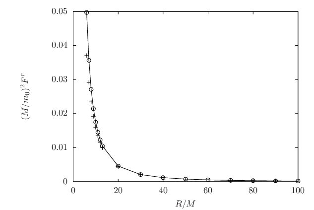
As discussed in Chapter 4, we can accelerate the convergence of the self-force regularization using a numerical fit to find the higher order regularization parameters. Figure 8.2 gives an example of this for , using the LAPACK least squares routine DGELSS [2]. The plot shows that the calculated self-force is consistent for a broad range of numerical fits. Similar plots could have been prepared for the other radii in Table 8.1, although the highest value of was decreased as the orbital radius increased. The higher order terms go through in (4.49).

For circular orbits, the radial component of the self-force is conservative and not dissipative. The temporal component is dissipative and should be offset by the energy flux of the gravitational waves [13]. The wave energy flux to infinity is (7.82) and the energy flux down the horizon is (7.90). From equation (4.55), the rate of energy loss due to the gravitational self-force is
| (8.3) |
where “sf” indicates that this is calculated using the self-force component . Table 8.2 shows that , to good precision. An example is . The energy flux to infinity is = and the energy flux down the horizon is =. The sum is =. The self-force gives an energy loss: =, which is opposite the wave energy flux. The offset occurs even though and are quadratic in the perturbation, while is linear in the perturbation.
| 6 | ||||
|---|---|---|---|---|
| 7 | ||||
| 8 | ||||
| 9 | ||||
| 10 | ||||
| 11 | ||||
| 12 | ||||
| 13 | ||||
| 20 | ||||
| 30 | ||||
| 40 | ||||
| 50 | ||||
| 60 | ||||
| 70 | ||||
| 80 | ||||
| 90 | ||||
| 100 | ||||
| 120 | ||||
| 150 |
Fujita and Tagoshi made precise numerical calculations of the outgoing energy flux carried by the gravitational waves for circular orbits using a different numerical method [42]. Table 8.3 shows good agreement between their results and calculations done using the methods described in this thesis, for .
| Thesis | Fujita and Tagoshi | ||
|---|---|---|---|
| 2 | 1 | ||
| 2 | 2 | ||
| 3 | 1 | ||
| 3 | 2 | ||
| 3 | 3 | ||
| 4 | 1 | ||
| 4 | 2 | ||
| 4 | 3 | ||
| 4 | 4 | ||
| 5 | 1 | ||
| 5 | 2 | ||
| 5 | 3 | ||
| 5 | 4 | ||
| 5 | 5 | ||
| 6 | 1 | ||
| 6 | 2 | ||
| 6 | 3 | ||
| 6 | 4 | ||
| 6 | 5 | ||
| 6 | 6 | ||
| 7 | 1 | ||
| 7 | 2 | ||
| 7 | 3 | ||
| 7 | 4 | ||
| 7 | 5 | ||
| 7 | 6 | ||
| 7 | 7 |
As discussed in Chapter 3, Detweiler and Poisson derived a different solution for the even parity multipole. Table 8.4 converts the self-force values in Table 8.1 to their equivalents, using equation (3.331). Figure 8.3 is a log-log plot comparing the different self-forces for .
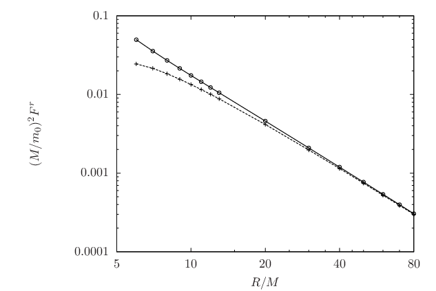
The self-force with the Detweiler-Poisson solution curves noticeably.
| 6 | 110 | ||
|---|---|---|---|
| 7 | 120 | ||
| 8 | 130 | ||
| 9 | 140 | ||
| 10 | 150 | ||
| 11 | 200 | ||
| 12 | 300 | ||
| 13 | 400 | ||
| 20 | 500 | ||
| 30 | 600 | ||
| 40 | 700 | ||
| 50 | 800 | ||
| 60 | 900 | ||
| 70 | 1000 | ||
| 80 | 10000 | ||
| 90 | 100000 | ||
| 100 | 1000000 |
Table 8.5 compares the radial self-force in Table 8.1 to the results of Barack and Sago, who did their calculations in the time domain by solving the field equations directly. They used the Detweiler-Poisson solution. Once this difference is taken into account, there is good agreement.
| (a) | (b) | Error (c) | (d) | |
|---|---|---|---|---|
| 6 | ||||
| 7 | ||||
| 8 | ||||
| 9 | ||||
| 10 | ||||
| 11 | ||||
| 12 | ||||
| 13 | ||||
| 20 | ||||
| 30 | ||||
| 40 | ||||
| 50 | ||||
| 60 | ||||
| 70 | ||||
| 80 | ||||
| 90 | ||||
| 100 | ||||
| 120 | ||||
| 150 |
The numerical results of this chapter show that the harmonic gauge solutions derived in this thesis can be used to accurately calculate the gravitational self-force for circular orbits. An effort was made to calculate the self-force for elliptic orbits. It is possible to calculate efficiently the waveforms and energy flux at infinity and near the event horizon. From the wave energy flux, the radiation reaction in an average sense can be calculated for elliptic orbits, but this approach does not give the self-force – including the conservative part – as such. To calculate the self-force, we need to evaluate the solutions along the orbit itself. Unfortunately, solutions along the orbit have larger oscillations than at infinity and the event horizon. As a result, the sum over the frequency index converges very slowly along an elliptic orbit, except at the turning points of the orbit. For the solutions to be useful for elliptic orbits, it seems necessary to regularize the retarded Green’s function in the frequency domain. This is left for future work, although numerical calculations show that the imaginary part of the Green’s function is small and finite. For circular orbits, the self-force components and do not require regularization. Numerical calculations show they are due entirely to the imaginary part of the spin retarded Green’s functions. Note that the imaginary part is a homogeneous solution of the Green’s function equation. Detweiler and Whiting showed that the self-force can be calculated from homogeneous solutions [35]. However, the imaginary part does not give the conservative component, , which must be due to the real part of the Green’s function. In a related area, Gralla and collaborators calculated the dissipative part of the scalar self-force for circular orbits using the imaginary part of the scalar Green’s function, which represents one-half the difference between the retarded and advanced solutions [48]. We must leave these issues and their application to elliptic orbits for future work.
Chapter 9 Conclusion
The main research result of this thesis consists of the harmonic gauge solutions derived in Chapters 2 and 3, using separation of variables and Fourier transforms. The solutions are written in terms of six functions of various spin weights, which satisfy decoupled ordinary differential equations. For odd parity, the solutions are given in terms of two generalized Regge-Wheeler functions, one with and one with . The even parity solutions contain the remaining four functions: three generalized Regge-Wheeler functions (two with and one with ) and the Zerilli function, which is related to the spin Regge-Wheeler function. The spin functions are gauge invariant and therefore physically meaningful. Gauge changes which preserve the harmonic gauge are implemented by adding homogeneous spin 1 and spin 0 solutions.
Chapter 4 discusses the background equations of motion and shows how the harmonic gauge solutions can be applied to calculate the gravitational self-force, which gives the first order perturbative corrections to the equations of motion for a small mass orbiting a much larger black hole. Chapter 5 provides Fourier transforms for the stress energy tensor. Chapter 6 shows how to solve the generalized Regge-Wheeler and Zerilli equations. Chapter 7 explains how to obtain expressions for gravitational waveforms and energy flux from the solutions derived in Chapters 2 and 3.
The harmonic gauge solutions yield accurate calculations of the gravitational self-force for circular orbits, as demonstrated in Chapter 8. However, there are open issues. The solution for circular orbits conflicts with the published Detweiler-Poisson solution for that multipole. As discussed at the end of Chapter 4, the discrepancy does not appear to affect gauge invariant observables, but nevertheless should be resolved. Another issue is how to calculate the gravitational self-force for elliptic orbits, and the problems here are briefly explained at the end of Chapter 8. Even if the harmonic gauge solutions derived in this thesis are not practical for additional numerical work, they still would be useful for analytic approximations, which in turn could further our understanding of the gravitational self-force.
References
- [1] M. Abramowitz and I. Stegun, editors. Handbook of Mathematical Functions. Dover Publications, New York, 1972.
- [2] E. Anderson, Z. Bai, C. Bischof, S. Blackford, J. Demmel, J. Dongarra, J. Du Croz, A. Greenbaum, S. Hammarling, A. McKenney, and D. Sorensen. LAPACK Users’ Guide. Society for Industrial and Applied Mathematics, Philadelphia, third edition, 1999.
- [3] G. Arfken. Mathematical Methods for Physicists. Academic Press, New York, third edition, 1985.
- [4] N. Ashby. Personal communication, as described at the end of the Introduction to this thesis.
- [5] N. Ashby. Planetary perturbation equations based on relativistic Keplerian motion. In J. Kovalevsky and V. Brumberg, editors, Relativity in Celestial Mechanics and Astrometry, page 41, Leningrad, 1985. IAU Symposium No. 114, Reidel, Netherlands, 1986.
- [6] L. Barack and C. Lousto. Computing the gravitational self-force on a compact object plunging into a Schwarzschild black hole. Phys. Rev. D, 66:061502(R), 2002.
- [7] L. Barack and C. Lousto. Perturbations of Schwarzschild black holes in the Lorenz gauge: Formulation and numerical implementation. Phys. Rev. D, 72:104026, 2005.
- [8] L. Barack, Y. Mino, H. Nakano, A. Ori, and M. Sasaki. Calculating the gravitational self-force in Schwarzschild spacetime. Phys. Rev. Lett., 88:091101, 2002.
- [9] L. Barack and A. Ori. Mode sum regularization approach for the self-force in black hole spacetime. Phys. Rev. D, 61:061502(R), 2000.
- [10] L. Barack and A. Ori. Gravitational self-force and gauge transformations. Phys. Rev. D, 64:124003, 2001.
- [11] L. Barack and A. Ori. Regularization parameters for the self-force in Schwarzschild spacetime: Scalar case. Phys. Rev. D, 66:084022, 2002.
- [12] L. Barack and A. Ori. Regularization parameters for the self-force in Schwarzschild spacetime. II. Gravitational case. Phys. Rev. D, 67:024029, 2003.
- [13] L. Barack and N. Sago. Gravitational self-force on a particle in circular orbit around a Schwarzschild black hole. Phys. Rev. D, 75:064021, 2007.
- [14] J. Bekenstein. Extraction of energy and charge from a black hole. Phys. Rev. D, 7:949, 1973.
- [15] L. Blanchet, B. Iyer, C. Will, and A. Wiseman. Gravitational waveforms from inspiralling compact binaries to second-post-Newtonian order. Class. Quantum Grav., 13:575, 1996.
- [16] R. Breuer, P. Chrzanowski, H. Hughes, and C. Misner. Geodesic synchroton radiation. Phys. Rev. D, 8:4309, 1973.
- [17] D. Brown, S. Fairhurst, B. Krishnan, R. Mercer, R. Kopparapu, L. Santamaria, and J. Whelan. Data formats for numerical relativity waves, September 2007. gr-qc/0709.0093v1.
- [18] A. Buonanno, G. Cook, and F. Pretorius. Inspiral, merger, and ring-down of equal-mass black-hole binaries. Phys. Rev. D, 75:124018, 2007.
- [19] A. Buonanno, Y. Pan, J. Baker, J. Centrella, B. Kelly, S. McWilliams, and J. van Meter. Toward faithful templates for non-spinning binary black holes using the effective-one-body approach, June 2007. gr-qc/0706.3732v1.
- [20] L. Burko. Self-force on a particle in orbit around a black hole. Phys. Rev. Lett., 84:4529, 2000.
- [21] B. Carlson. Computing elliptic integrals by duplication. Numer. Math., 33:1, 1979.
- [22] S. Chandrasekhar. The Mathematical Theory of Black Holes. Oxford University Press, New York, 1992.
- [23] E. Ching, P. Leung, W. Suen, and K. Young. Wave propagation in gravitational systems: late time behavior. Phys. Rev. D, 52:2118, 1995.
- [24] P. Chrzanowski. Vector potential and metric perturbations of a rotating black hole. Phys. Rev. D, 11:2042, 1975.
- [25] P. Chrzanowski and C. Misner. Geodesic synchrotron radiation in the Kerr geometry by the method of asymptotically factorized Green’s functions. Phys. Rev. D, 10:1701, 1974.
- [26] C. Cunningham, R. Price, and V. Moncrief. Radiation from collapsing relativistic stars. I. Linearized odd-parity radiation. Astrophys. J., 224:643, 1978.
- [27] C. Cutler, L. Finn, E. Poisson, and G. Sussman. Gravitational radiation from a particle in circular orbit around a black hole. II. Numerical results for the nonrotating case. Phys. Rev. D, 47:1511, 1993.
- [28] C. Cutler, D. Kennefick, and E. Poisson. Gravitational radiation reaction for bound motion around a Schwarzschild black hole. Phys. Rev. D, 50:3816, 1994.
- [29] C. Darwin. The gravity field of a particle. Proc. R. Soc. A, 249:180, 1959.
- [30] C. Darwin. The gravity field of a particle. II. Proc. R. Soc. A, 263:39, 1961.
- [31] M. Davis, R. Ruffini, and J. Tiomno. Pulses of gravitational radiation of a particle falling radially into a Schwarzschild black hole. Phys. Rev. D, 5:2932, 1972.
- [32] S. Detweiler. Perspective on gravitational self-force analyses. Class. Quantum Grav., 22:S681, 2005.
- [33] S. Detweiler, E. Messaritaki, and B. Whiting. Self-force of a scalar field for circular orbits about a Schwarzschild black hole. Phys. Rev. D, 67:104016, 2003.
- [34] S. Detweiler and E. Poisson. Low multipole contributions to the gravitational self-force. Phys. Rev. D, 69:084019, 2004.
- [35] S. Detweiler and B. Whiting. Self-force via a Green’s function decomposition. Phys. Rev. D, 67:024025, 2003.
- [36] B. DeWitt and R. Brehme. Radiation damping in a gravitational field. Ann. of Phys. (N.Y.), 9:220, 1960.
- [37] L. Diaz-Rivera, E. Messaritaki, B. Whiting, and S. Detweiler. Scalar field self-force effects on orbits about a Schwarzschild black hole. Phys. Rev. D, 70:124018, 2004.
- [38] S. Drasco, É. Flanagan, and S. Hughes. Computing inspirals in Kerr in the adiabatic regime: I. The scalar case. Class. Quantum Grav., 22:S801, 2005.
- [39] S. Drasco and S. Hughes. Gravitational wave snapshots of generic extreme mass ratio inspirals. Phys. Rev. D, 73:024027, 2006.
- [40] D. Eardley, D. Lee, and A. Lightman. Gravitational-wave observations as a tool for testing relativistic gravity. Phys. Rev. D, 8:3308, 1973.
- [41] D. Eardley, D. Lee, A. Lightman, R. Wagoner, and C. Will. Gravitational-wave observations as a tool for testing relativistic gravity. Phys. Rev. Lett., 30:884, 1973.
- [42] R. Fujita and H. Tagoshi. New numerical methods to evaluate homogeneous solutions of the Teukolsky equation. Prog. Theor. Phys., 112:415, 2004.
- [43] D. Gal’tsov. Radiation reaction in the Kerr gravitational field. J. Phys. A, 15:3737, 1982.
- [44] U. Gerlach and U. Sengupta. Gauge-invariant perturbations on most general spherically symmetric space-times. Phys. Rev. D, 19:2268, 1979.
- [45] K. Glampedakis and D. Kennefick. Zoom and whirl: Eccentric equatorial orbits around spinning black holes and their evolution under gravitational radiation reaction. Phys. Rev. D, 66:044002, 2002.
- [46] J. Goldberg. Invariant transformations and Newman-Penrose constants. J. Math. Phys., 8:2161, 1967.
- [47] J. Goldberg, A. Macfarlane, E. Newman, F. Rohrlich, and E. Sudarshan. Spin- spherical harmonics and . J. Math. Phys., 8:2155, 1967.
- [48] S. Gralla, J. Friedman, and A. Wiseman. Numerical radiation reaction for a scalar charge in Kerr circular orbit, February 2005. gr-qc/0502123v1.
- [49] D. Griffiths. Introduction to Quantum Mechanics. Prentice-Hall, New Jersey, 1995.
- [50] A. Hamilton. Perturbation theory of spherically symmetric self-similar black holes, November 2007. gr-qc/0706.3238v2 (personal communication).
- [51] J. Hartle. Gravity. Addison-Wesley, San Francisco, 2003.
- [52] S. Hawking and J. Hartle. Energy and angular momentum flow into a black hole. Commun. Math. Phys., 27:283, 1972.
- [53] W. Hikida, H. Nakano, and M. Sasaki. Self-force regularization in the Schwarzschild spacetime. Class. Quantum Grav., 22:S753, 2005.
- [54] J. Hobbs. A vierbein formalism of radiation damping. Ann. of Phys. (N.Y.), 47:141, 1968.
- [55] S. Hughes. Computing radiation from Kerr black holes: Generalization of the Sasaki-Nakamura equation. Phys. Rev. D, 62:044029, 2000. ibid. 67:089902(E), 2003 (Erratum).
- [56] S. Hughes. Evolution of circular, nonequatorial orbits of Kerr black holes due to gravitational-wave emission. Phys. Rev. D, 61:084004, 2000. ibid. 63:049902(E), 2001, ibid. 65:069902(E), 2002, ibid. 67:089901(E), 2003 (Errata).
- [57] S. Hughes, S. Drasco, É. Flanagan, and J. Franklin. Gravitational radiation reaction and inspiral waveforms in the adiabatic limit. Phys. Rev. Lett., 94:221101, 2005.
- [58] R. Isaacson. Gravitational radiation in the limit of high frequency. I. The linear approximation and geometrical optics. Phys. Rev., 166:1263, 1968.
- [59] R. Isaacson. Gravitational radiation in the limit of high frequency. II. Nonlinear terms and the effective stress tensor. Phys. Rev., 166:1272, 1968.
- [60] J. Jackson. Classical Electrodynamics. John Wiley, New York, second edition, 1975.
- [61] S. Jhingan and T. Tanaka. Improvement on the metric reconstruction scheme in the Regge-Wheeler-Zerilli formalism. Phys. Rev. D, 67:104018, 2003.
- [62] E. Leaver. Solutions to a generalized spheroidal wave equation. J. Math. Phys., 27:1238, 1986.
- [63] E. Leaver. Spectral decomposition of the perturbation response of the Schwarzschild geometry. Phys. Rev. D, 34:384, 1986. ibid. 38:725, 1988 (Erratum).
- [64] S. Leonard and E. Poisson. Radiative multipole moments of integer-spin fields in curved spacetime. Phys. Rev. D, 56:4789, 1997.
- [65] K. Martel. Gravitational waveforms from a point particle orbiting a Schwarzschild black hole. Phys. Rev. D, 69:044025, 2004.
- [66] K. Martel and E. Poisson. Gravitational perturbations of the Schwarzschild spacetime: A practical covariant and gauge-invariant formalism. Phys. Rev. D, 71:104003, 2005.
- [67] J. Mathews and R. Walker. Mathematical Methods of Physics. Addison-Wesley, New York, second edition, 1970.
- [68] Y. Mino, H. Nakano, and M. Sasaki. Covariant self-force regularization of a particle orbiting a Schwarzschild black hole. Prog. Theor. Phys., 108:1039, 2002.
- [69] Y. Mino, M. Sasaki, M. Shibata, H. Tagoshi, and T. Tanaka. Black hole perturbation. Prog. Theor. Phys. Suppl., 128:1, 1997.
- [70] Y. Mino, M. Sasaki, and T. Tanaka. Gravitational radiation reaction to a particle motion. Phys. Rev. D, 55:3457, 1997.
- [71] C. Misner, K. Thorne, and J. Wheeler. Gravitation. W. H. Freeman, New York, 1973.
- [72] V. Moncrief. Gravitational perturbations of spherically symmetric systems. I. The exterior problem. Ann. of Phys. (N.Y.), 88:323, 1974.
- [73] V. Moncrief. Odd-parity stability of a Reissner-Nordström black hole. Phys. Rev. D, 9:2707, 1974.
- [74] V. Moncrief. Stability of Reissner-Nordström black holes. Phys. Rev. D, 10:1057, 1974.
- [75] A. Nagar and L. Rezzolla. Gauge-invariant non-spherical metric perturbations of Schwarzschild black-hole spacetimes. Class. Quantum Grav., 22:R167, 2005. ibid. 23:4297, 2006 (Corrigendum).
- [76] T. Nakamura and H. Tagoshi. Gravitational waves from a point particle in circular orbit around a black hole: Logarithmic terms in the post-Newtonian expansion. Phys. Rev. D, 49:4016, 1994.
- [77] H. Nakano, N. Sago, and M. Sasaki. Gauge problem in the gravitational self-force: First post-Newtonian force in the Regge-Wheeler gauge. Phys. Rev. D, 68:124003, 2003.
- [78] E. Newman and R. Penrose. An approach to gravitational radiation by a method of spin coefficients. J. Math. Phys., 3:566, 1962. ibid. 4:998, 1963 (Errata).
- [79] E. Newman and R. Penrose. Note on the Bondi-Metzner-Sachs group. J. Math. Phys., 7:863, 1966.
- [80] LISA Mission Science Office. LISA: Probing the Universe with Gravitational Waves. LISA Mission Science Office, 1.0 edition, 2007.
- [81] A. Ori. Harmonic-gauge dipole metric perturbations for weak-field circular orbits in Schwarzschild spacetime. Phys. Rev. D, 70:124027, 2004.
- [82] P. Peters. Gravitational radiation and the motion of two point masses. Phys. Rev., 136:B1224, 1964.
- [83] P. Peters and J. Mathews. Gravitational radiation from point masses in a Keplerian orbit. Phys. Rev., 131:435, 1963.
- [84] E. Poisson. Gravitational radiation from a particle in circular orbit around a black hole. I. Analytical results for the nonrotating case. Phys. Rev. D, 47:1497, 1993.
- [85] E. Poisson. Absorption of mass and angular momentum by a black hole: Time-domain formalisms for gravitational perturbations, and the small-hole or slow-motion approximation. Phys. Rev. D, 70:084044, 2004.
- [86] E. Poisson. The motion of point particles in curved spacetime. Living Rev. Relativity, 7(6), May 2004. Cited December 9, 2006. http://www.livingreviews.org/lrr-2004-6.
- [87] E. Poisson. A Relativist’s Toolkit. Cambridge University Press, New York, 2004.
- [88] A. Polyanin and V. Zaitsev. Handbook of Exact Solutions for Ordinary Differential Equations. CRC Press, New York, second edition, 2003.
- [89] A. Pound and E. Poisson. Multi-scale analysis of the electromagnetic self-force in a weak gravitational field, August 2007. gr-qc/0708.3037v1.
- [90] A. Pound and E. Poisson. Osculating orbits in Schwarzschild spacetime, with an application to extreme mass-ratio inspirals, August 2007. gr-qc/0708.3033v1.
- [91] A. Pound, E. Poisson, and B. Nickel. Limitations of the adiabatic approximation to the gravitational self-force. Phys. Rev. D, 72:124001, 2005.
- [92] W. Press and S. Teukolsky. Perturbations of a rotating black hole. II. Dynamical stability of the Kerr metric. Astrophys. J., 185:649, 1973.
- [93] W. Press and S. Teukolsky. Perturbations of a rotating black hole. III. Interaction of the hole with gravitational and electromagnetic radiation. Astrophys. J., 193:443, 1974.
- [94] W. Press, S. Teukolsky, W. Vetterling, and B. Flannery. Numerical Recipes in Fortran 77. Cambridge University Press, New York, second edition, 1992.
- [95] R. Price and K. Thorne. Non-radial pulsation of general-relativistic stellar models. II. Properties of the gravitational waves. Astrophys. J., 155:163, 1969.
- [96] T. Quinn and R. Wald. Axiomatic approach to electromagnetic and gravitational radiation reaction of particles in curved spacetime. Phys. Rev. D, 56:3381, 1997.
- [97] T. Quinn and R. Wald. Energy conservation for point particles undergoing radiation reaction. Phys. Rev. D, 60:064009, 1999.
- [98] T. Regge and J. Wheeler. Stability of a Schwarzschild singularity. Phys. Rev., 108:1063, 1957.
- [99] E. Rosenthal. Regularization of the second-order gravitational perturbations produced by a compact object. Phys. Rev. D, 72:121503(R), 2005.
- [100] E. Rosenthal. Construction of the second-order gravitational perturbations produced by a compact object. Phys. Rev. D, 73:044034, 2006.
- [101] E. Rosenthal. Second-order gravitational self-force. Phys. Rev. D, 74:084018, 2006.
- [102] N. Sago, H. Nakano, and M. Sasaki. Gauge problem in the gravitational self-force: Harmonic gauge approach in the Schwarzschild background. Phys. Rev. D, 67:104017, 2003.
- [103] J. Sakurai. Modern Quantum Mechanics. Addison-Wesley, New York, revised edition, 1994.
- [104] B. Schutz. A First Course in General Relativity. Cambridge University Press, New York, 1990.
- [105] T. Tanaka, M. Shibata, M. Sasaki, H. Tagoshi, and T. Nakamura. Gravitational wave induced by a particle orbiting around Schwarzschild black hole. Prog. Theor. Phys., 90:65, 1993.
- [106] S. Teukolsky. Perturbations of a rotating black hole. I. Fundamental equations for gravitational, electromagnetic and neutrino-field perturbations. Astrophys. J., 185:635, 1973.
- [107] K. Thorne. Multipole expansions of gravitational radiation. Rev. Mod. Phys., 52:299, 1980.
- [108] C. Vishveshwara. Stability of the Schwarzschild metric. Phys. Rev. D, 1:2870, 1970.
- [109] R. Wald. On perturbations of a Kerr black hole. J. Math. Phys., 14:1453, 1973.
- [110] S. Weinberg. Gravitation and Cosmology. John Wiley, New York, 1972.
- [111] J. Wheeler. Geons. Phys. Rev., 97:511, 1955.
- [112] S. Wolfram. The Mathematica Book. Wolfram Research, 2005. From the help browser for Mathematica, version 5.2.
- [113] R. Zare. Angular Momentum. John Wiley, New York, 1988.
- [114] F. Zerilli. The Gravitational Field of a Particle Falling in a Schwarzschild Geometry Analyzed in Tensor Harmonics. PhD thesis, Princeton University, 1969.
- [115] F. Zerilli. Gravitational field of a particle falling in a Schwarzschild geometry analyzed in tensor harmonics. Phys. Rev. D, 2:2141, 1970.
- [116] F. Zerilli. Tensor harmonics in canonical form for gravitational radiation and other applications. J. Math. Phys., 11:2203, 1970.
- [117] D. Zill. A First Course in Differential Equations. PWS-KENT Publishing Company, Boston, fifth edition, 1993.
Appendix A Non-Zero Frequency Even Parity Solutions for
Listed below are the non-zero frequency even parity solutions and their radial derivatives, for . The derivation of these solutions is covered in subsection 3.1.1.
| (A.1) |
| (A.2) |
| (A.3) |
| (A.4) |
| (A.5) |
| (A.6) |
| (A.7) |
| (A.8) |
| (A.9) |
| (A.10) |
| (A.11) |
| (A.12) |
| (A.13) |
| (A.14) |
Appendix B Five Zero Frequency Even Parity Solutions for
Listed below are five zero frequency even parity solutions and their radial derivatives, for . The five are , , , and . The derivation of these functions and the expressions for and are given in subsection 3.2.1.
| (B.1) |
| (B.2) |
| (B.3) |
| (B.4) |
| (B.5) |
| (B.6) |
| (B.7) |
| (B.8) |
| (B.9) |
| (B.10) |
Appendix C Zero Frequency Even Parity Solution for
| (C.3) |
| (C.4) |
where
| (C.5) |
| (C.6) |
The function is defined in equation (3.158).
Appendix D Zero Frequency Even Parity Solutions for
Listed below are the zero frequency even parity solutions , and , and their radial derivatives, for . Also for this mode, we have and . The derivation of these solutions is in subsection 3.2.4.
| (D.1) |
| (D.2) |
| (D.3) |
| (D.4) |
| (D.5) |
| (D.6) |
*