Finite Approximations of Switched Homogeneous Systems for Controller Synthesis
Abstract
We demonstrate the use of a new, control-oriented notion of finite state approximation for a particular class of hybrid systems. Specifically, we consider the problem of designing a stabilizing binary output feedback switching controller for a pair of unstable homogeneous second order systems. The constructive approach presented in this note, in addition to yielding an explicit construction of a deterministic finite state approximate model of the hybrid plant, allows us to efficiently establish a useable upper bound on the quality of approximation, and leads to a discrete optimization problem whose solution immediately provides a certifiably correct-by-design controller for the original system. The resulting controller consists of a finite state observer for the plant and a corresponding full state feedback switching control law.
1 Introduction
1.1 Motivation and Overview
Finite state approximations and abstractions of hybrid plants have been explored as a means for addressing instances in which the interaction between analog and discrete dynamics11 1 “Analog” and “discrete” here refer to whether the dynamics evolve in a continuous or a discrete state-space; the independent variable, time, may be continuous or discrete in either case. leads to complex analysis and synthesis problems that cannot be adequately handled by traditional methods. Some of the early work in this area explored the use of ‘qualitative’ models, namely non-deterministic automata whose output behavior contains that of the original hybrid system [19]. In [21], an approach for deriving non-deterministic finite state approximations of systems with quantized outputs was proposed and used in conjunction with the supervisory control theory developed by Ramadge and Wonham [22] to design controllers meeting the desired specifications. Another line of research, inspired by formal verification techniques in computer science, explored the construction of deterministic discrete abstractions of hybrid systems [2]. Early work in this area focused on identifying classes of systems that admit finite bisimulation abstractions [11, 15]. Having recognized that these classes are fairly limited, more recent work has focused on finding discrete abstractions that are related to the original hybrid system by an approximate simulation or bisimulation relation [10, 25, 26]. The resulting controller design problem is then a two step procedure in which a finite state supervisory controller is first designed, and subsequently refined to yield a certified hybrid controller for the original plant [27].
In this note, we demonstrate the use of a new22 2 Preliminary versions of this work were presented in [32, 29, 30]., alternative notion of approximation that, in addition to yielding a finite state deterministic approximate model of the original hybrid system, allows one to efficiently establish a useable upper bound on the quality of approximation, and leads to a discrete optimization problem whose solution immediately provides a certifiably correct-by-design (finite state) controller for the original system. The notion of finite input/output approximation employed in this note is thus potentially better suited to the purpose of control design than the existing methods since it allows for a streamlined and efficient synthesis procedure. Another promising development is that, in contrast to many of the existing methods and our early work on this problem, we have succeeded in approximating unstable systems by finite state automata for the purpose of control design.
We demonstrate this approach in a particular setting, namely for the problem of designing a stabilizing, binary output feedback, switching controller for a pair of unstable, homogeneous, second order systems. This problem was specifically chosen because several of its simpler formulations have been extensively studied and are well understood [7, 17]. Necessary and sufficient conditions for stability of switched second order homogeneous systems were derived in [9]. A Lyapunov based approach for designing stabilizing full state feedback switching controllers for second order homogenous systems was proposed in [12]. While the results available for general homogeneous systems remain limited, the special case of switched linear systems has been more extensively studied. For instance, in the linear full state feedback analog case, the existence of a Hurwitz convex combination (, ) of a given pair of unstable state matrices ( and ) is known to be a necessary [8] and sufficient [34] condition for the existence of a quadratically stabilizing switching controller. The switching controller can take on a variety of forms in this case (time-switched controller, hybrid controller, etc…). In particular, when has a real eigenvalue, a quadratic switching surface and corresponding state dependent variable structure control law [13] can be designed to stabilize the system [34]. In this case, once designed assuming full state feedback, the stabilizing controller can be exactly implemented by transmitting appropriately chosen binary state information from the plant to the controller, namely information that the state is currently in one or the other region of the state-space. Lyapunov based approaches have also been extended to time-sampled versions of the problem [6, 18], and to the output feedback case [24]: Typically the output is assumed to be a linear function of the state, and the resulting controller is observer-based [8]. In contrast, the setting considered in this note where fixed, binary sensors are used leads to a more difficult state estimation (and thus controller synthesis) problem33 3 This setup differs significantly from the variable structure controller setup described above, as the binary sensors are assumed to be fixed a priori with no regard to the system dynamics. As such, there generally is a mismatch between the information provided by the sensors and the binary information needed to implement a variable structure switching law. The resulting state estimation problem is at the core of the design challenge here.. This case has been much less well studied, and has only begun to receive attention in the recent past [4, 20, 23]. Specifically, the use of finite state approximations in this context remains minimally explored.
The constructive controller synthesis approach can be summarized as follows: First, the plant is approximated by a deterministic finite state machine and a usable bound on the quality of approximation is efficiently established. Next, a switching control law is designed to robustly stabilize the nominal finite state machine model in the presence of admissible approximation uncertainty. The resulting controller, which is thus certifiably correct-by-design, is then also a finite state system. Additionally, the procedure by which it is synthesized is computationally tractable in the sense that it is based on a finite state nominal model.
Practically, this design approach may be utilized in applications where very coarse sensors are used to keep operating cost, weight or power consumption low. Looking ahead, having a systematic procedure for designing control systems specifically for the case where the plant and controller interact through finite alphabets points to new paradigms for control over networks in which the amount of information to be encoded and transmitted over communication channels is significantly reduced. Finally, this design procedure may be employed by artificially imposing coarse measurements on a switched system for which there is no other available or tractable approach for synthesizing controllers, though the relevant question of how to best impose a finite measurement quantization for the control objective of interest is not addressed in this paper.
1.2 Organization of the Paper
The paper is organized as follows: The statement of the control design problem and an overview of the controller design procedure are described in Section 2. The algorithms proposed for constructing a finite state approximation of the plant, and for computing an a-posteriori bound on the resulting approximation error are presented in Section 3. Design of the robust stabilizing switching law and the structure of the resulting switching controller are addressed in Section 4. Illustrative examples are presented in Section 5. The paper concludes in Section 6, where recommendations for future work are given.
1.3 Notation
The notation used in the paper is fairly standard: , and denote the sets of non-negative integers, reals and non-negative reals, respectively. For real interval , denotes the length of . Given a vector , denotes its transpose and denotes its Euclidean norm. Given sets and , denotes the cardinality of , denotes their Cartesian product, denotes the set of all infinite sequences taking their values in set and (boldface) denotes an element of . Given a function and a proper subset , denotes the restriction of to , that is the function defined by for . Given two functions and , their composition, denoted by , is a function defined by . Given two real-valued functions and , the notation is understood to mean that for all .
2 Problem Statement & Overview of the Design Procedure
2.1 Problem Statement
Consider a discrete-time plant described by
| (1) |
| (2) |
| (3) |
where the time index , state , performance output , and control input is binary with . Sensor output is also taken to be binary, , with the understanding that when , is taken to be in one quadrant and in the other. Functions and vector , , are given. The following conditions are assumed to hold for each :
- 1.
is continuous.
- 2.
is homogeneous with degree 1: That is, for all , .
In this setup, the effect of the control action is to pick a choice of system from a given pair and to hold that choice until the next time step, at which point a new measurement is available and a new choice of system is made and implemented.
The objective is to design a controller such that the closed loop system with output (Figure 1) satisfies the following performance objective for some , for any initial condition of plant :
| (4) |
Satisfaction of this performance objective guarantees that the state of the closed loop system (globally) exponentially converges to the origin, on average, at a rate not less than .

2.2 Overview of the Controller Design Procedure
Design of the stabilizing controller is an iterative procedure, with each iteration consisting of a sequence of steps. First, the plant is approximated by the interconnection of a finite state machine and a complex system representing the approximation error (Figure 2). Next, a meaningful and useable “gain bound” is established for the approximation error, system . Finally, an attempt is made to synthesize a feedback switching law for the nominal finite state model , that is robust to the approximation error . If synthesis is successful, the resulting controller is guaranteed to globally exponentially stabilize the plant at some verified rate . Otherwise if synthesis is unsuccessful, or if the verified rate is unsatisfactory, a more refined approximation (meaning a finite state machine with a larger number of states) is sought for the plant and the above process is repeated.

3 A Finite State Approximation of the Plant
A deterministic finite state machine (DFM for short) is understood to be a discrete-time dynamical system (independent variable ) described by a state transition equation (5) and an output equation (6)
| (5) | |||||
| (6) |
State , input , and output , where , and are finite state, input alphabet and output alphabet sets, respectively.
3.1 A Notion of Approximation
Given a plant with binary control input , binary sensor output and upper bounded44 4 It will become clear in Section 3.2 that is indeed upper bounded for the class of systems under consideration. performance output . Consider a system with inputs and , and with outputs , and , where is a finite discrete subset of . Suppose that has the internal structure shown in Figure 3, where is a deterministic finite state machine. To ensure well-posedness, we require that there be no direct feedthrough from input to output in : In other words, is only allowed to be a function of the input and the state of at time . Memoryless system is defined by
System is thus a deterministic finite state machine.
Consider also the corresponding system shown in Figure 4. Memoryless system is defined by
System is not a deterministic finite state machine in general, unless plant is one. Moreover, the existing requirement that there be no direct feedthrough from to in ensures that the outputs of and of cannot be trivially matched.

Now consider the interconnection, as in Figure 2, of and with these particular structures, and suppose that the two copies of are identically initialized. Regardless of the choice of , it can be seen by direct inspection that for arbitrary initial conditions of and for any input , the corresponding outputs of and of are identical.
Suppose that we can construct such that the following two conditions are satisfied for any input and any initial condition of :
- 1.
Outputs of the interconnection and of satisfy
(7) - 2.
For and defined by , there exists a constant such that every feasible input/output pair of signals of the error system satisfies the gain condition:
(8)
The resulting deterministic finite state machine is then said to be a finite state approximation of , and the corresponding system is said to be the approximation error. The following remarks aim to clarify the reasoning behind this approach to plant approximation.

Remark 1
The structure of the approximation error proposed in this setting is significantly different from that of the approximation error in the traditional stable LTI model reduction setting. In that setting, a stable lower order LTI model is considered to be a good approximation of the original stable LTI system if the outputs of the two systems are not too different, in a worst case sense, when driven side by side by the same input. The structure proposed here, where the output of the plant is fed back to , is needed because the original system is not stable: Two copies of initialized differently and driven side by side may end up with different outputs at every step. Thus, there is a need to explicitly ’estimate’ the initial condition of , otherwise there is no hope for satisfying gain condition (8) for any choice of .
Remark 2
The first condition characterizing a valid finite state approximation, namely the inequality in (7), is motivated by the control objective (4) at hand. In particular, if (7) holds and a controller is designed to ensure that the closed loop system satisfies the auxiliary performance objective
| (9) |
then a corresponding controller implemented in feedback with plant is guaranteed to satisfy performance objective (4): We will return to address this statement in more detail in Section 4. Upper boundedness of signal ensures that (7) can always be satisfied for some appropriate finite choice of . Intuitively, a better approximation in which the instantaneous difference between and is smaller is desirable and leads to a less conservative controller design.
Remark 3
The second condition characterizing a valid finite state approximation, namely the ’gain condition’ describing the approximation error , is compatible with the framework and the tools for robustness analysis of systems over finite alphabets developed in [31]. The choice of functions and proposed here are specific to the control objective at hand. In particular, the smallest value of for which (8) holds (the ’gain’ of ) represents the fraction of time (computed over an infinite window) that the outputs of and disagree in the worst-case scenario. A smaller value of is thus desirable and indicative of a better approximation.
In the following sections, a constructive procedure for generating a viable and a computationally efficient algorithm for computing an a-posteriori upper bound on the gain of the resulting error system are proposed.
3.2 Construction of the Nominal Model
The approach proposed for constructing a nominal finite state model to approximate plant takes advantage of the dynamical properties specific to homogeneous systems, evident after a coordinate transformation; interested readers are referred to [28] for an overview of other potential approaches. Let
In a polar coordinate system where and , the dynamics of system described in (1), (2) and (3) are given by:
| (10) |
| (11) |
| (12) |
where
This coordinate transformation highlights two important properties of the class of systems under consideration:
- 1.
The evolutions of the angular coordinate and of both outputs of are independent of the radial coordinate : The state of the system relevant to the stabilization problem at hand effectively evolves on the unit circle.
- 2.
For brevity of notation in the following argument, denote the composition simply by . For each , we have , , where and are again compact in since each is continuous. Thus we have
and
It thus follows that is upper bounded.
Compactness of the effective state set and upper boundedness of the performance output are instrumental in ensuring that this class of plants is amenable to a finite state approximation.
is constructed by partitioning the unit circle into a collection of intervals and defining the potential states of to correspond to the intervals and the unions of adjacent intervals. This partition generally need not consist of equal length intervals; however, it should be chosen such that the outputs associated with all the (analog) states of whose angular coordinates lie in any given interval are identical, in order to avoid introducing unnecessary uncertainty.
In particular, consider a partition of the unit circle consisting of intervals where for some sequence of angles satisfying:
The number and choice of angles is a design parameter here.
Construct a set of intervals on the unit circle:
where is the set of all ” adjacent intervals”. That is:
This set , consisting of distinct elements, is the set of all potential states of . It will become clear shortly that continuity of rules out the union of two non-adjacent quantization intervals from being a potential state of in this setup.
For , let
and
Note that and , by construction. For , , let
and
Remark 4
It follows from the continuity of that for any choice of and , is a single connected interval. Thus
is an interval of the form , in other words, an element of .
The dynamics of are then given by
| (13) | |||||
with , and defined by
In particular, let denote the potential state corresponding to the whole unit circle, that is . It is shown in the following Lemma that condition (7) is satisfied provided is initialized to this state.
Lemma 1
Proof 3.1.
Let and denote the states of and , respectively, at time . It follows from the construction of that:
- 1.
- 2.
We have . When is initialized to , , hence and . The statement of the Lemma thus follows by induction on .
Since the initial state of will be fixed to , the actual states of consist of those states in that are reachable from . The problem of computing the reachable subset can be recast as either one of two well-studied problems: (i) A one-to-all network shortest path problem, which can be efficiently solved (polynomial time in ) using any of the available shortest path algorithms (Dijkstra’s, Bellman-Ford, ) [1], or (ii) the problem of computing the accessible states of an automaton, which can be efficiently solved by constructing the transition tree of the automaton [16]. Thus any of a standard collection of algorithms can be used to compute ; interested readers are referred to the above two references for details of the various algorithms.
The dynamics of are thus given by:
| (15) | |||||
where the state transition function and output functions are given by and , , respectively.
3.3 Description of the Approximation Error
In this section, a procedure for computing an upper bound on the gain of the error system associated with a given plant and a corresponding nominal finite state model , constructed as described in the previous section, is presented. As before, refers to the actual states of .
Lemma 3.2.
If there exists a function and a such that
| (16) |
holds for all , and , where defined by:
then the error system with is initialized to satisfies (8) for that choice of .
Proof 3.3.
By summing up (16) along any state trajectory of from to , we get:
Hence, we have:
It follows from Lemma 1 that when is initialized to , we have for all , where and are the states of and , respectively. Thus, when or , and . Otherwise . Hence for all and all feasible input/output signal pairs of satisfy (8).
An upper bound for the gain of can thus be computed by solving a linear program in which we minimize such that (16) holds for all , and . This linear program has decision variables and inequality constraints, where .
Remark 3.4.
Recall that the approximation error is a complex system with both continuous and discrete states. Thus the appeal of this approach to computing a gain bound for is its simplicity and its computational efficiency. The downside of this approach is that it results in conservative gain bounds, for two reasons:
- 1.
It inherently assumes that an error occurs every single time it can.
- 2.
It assumes that all signal pairs are valid input sequences for , which is not the case since is an output of corresponding to .
Thus, in using this approach, we are in effect trading off simplicity and efficiency versus conservatism.
4 Controller Design
4.1 Two Related Synthesis Problems

Consider the following two controller synthesis problems:
-
Problem 2: Given a plant as in (1), (2) and (3) and a finite state approximation of constructed as described in Section 3.2 with the corresponding error system satisfying gain condition (8) for some . Design a full state feedback control law such that the interconnection shown in Figure 5 satisfies the auxiliary robust performance objective
for some , for all systems satisfying gain condition (8).
Problem 1 is the original problem of interest. Satisfaction of performance objective (4) guarantees that the state of the closed loop system globally exponentially converges to the origin, on average, at a rate not less than . To see that, note that this performance objective can be equivalently re-written as
where with
when the plant is initialized to . The largest value of for which (9) holds is then the guaranteed rate of exponential55 5 The notion of exponential convergence considered here is slightly different than that of global exponential convergence defined in standard textbooks such as [33, 14]; in particular, we are not requiring the term to be uniformly bounded. convergence; the actual rate of convergence may be (significantly) better.
Problem 2 is of interest as its solution provides a solution for Problem 1. In particular, let be a full state feedback controller such that satisfies (9) for some , for all admissible . Recall that by construction, the outputs of and of satisfy (7) whenever the same input drives the plant and the interconnection . Thus, to ensure that (4) holds for interconnection whenever (9) holds, it is sufficient to ensure that the controller connected in feedback with plant is identical to the subsystem with input and output in the interconnection . The structure of the resulting controller is shown in Figure 6: thus consists of , a deterministic finite state machine ”observer” for the plant and , a corresponding full state feedback control law.

4.2 Design of a Full State Feedback Robust Switching Law
The following problem is addressed in this section: Given a deterministic finite state machine with state set , a scalar , and an uncertainty class
Design a robust switching law such that the closed loop system shown in Figure 5 satisfies the auxiliary robust performance objective
for some , for all admissible uncertainty .
The robust switching law will be designed using dynamic programming techniques and a “small gain” argument. Consider the feedback interconnection of two systems and as in Figure 7. The ’Small Gain Theorem’ (Theorem 4.5) and Corollary 4.6, presented here without proof, are directly adapted from Theorem 1 and Remark 4, respectively, in [31].
Theorem 4.5.
(A ’Small Gain’ Theorem) Suppose that satisfies
| (17) |
for some and , where , , and are finite sets, and that satisfies
| (18) |
for some and . Then the interconnected system with input and output satisfies
| (19) |
for and defined by

Corollary 4.6.
It follows from Theorem 4.5 and Corollary 4.6 that the objective in (9) can be achieved by designing a switching law such that the feedback interconnection satisfies (17) with
| (20) | |||||
for some and , for and defined as in (8). Note that the exogenous input can be assumed to be constant here (representing the desired rate of convergence).
With the auxiliary robust performance objective reformulated as a design objective for system , the design of the full state feedback switching law can be carried out by solving a min-max optimization problem using standard dynamic programming techniques [5, 3]. The following theorem precisely formulates this approach: In this setting, function and operator play the role of the “cost-to-go” function and the “dynamic programming” operator, respectively. Value iteration is used to solve for the cost-to-go function, and the sought full state feedback switching law is then simply the optimizing argument. For the sake of completeness, a proof is outlined in the Appendix.
Theorem 4.7.
Consider a deterministic finite state machine with state transition equation
where is the state set and and are the input sets. Let be a given function. The following three statements are equivalent:
- (a)
There exists a such that the closed loop system satisfies
(21) - (b)
There exists a function such that the inequality
(22) holds for any , for defined by
(23) - (c)
The sequence of functions , , defined recursively by
(24) converges.
For the particular control problem of interest, the cost function
involves two parameters, the convergence rate and the small gain scaling parameter . Ultimately, the goal is to maximize for which there exists a and a such that (22) holds. However, since it is not possible to directly compute the optimal value of , a numerical search is carried out yielding a suboptimal value of : First, a range of values of for which the design objective can be met when is computed. Different values of are then sampled in this range to compute the largest feasible corresponding value of , with the largest of those being the (suboptimal) guaranteed rate of convergence.
5 Illustrative Examples
An academic example is presented in this section to illustrate the proposed design procedure. The example was chosen for its simplicity and amenability to analysis in the ideal (full state feedback) case, thus allowing us to numerically compare the performance of our finite state controllers in the binary sensing setting to the best achievable performance in the ideal setting for a given pair of plants.
Consider a harmonic oscillator
described in polar coordinates by
When , and the state trajectories are concentric circles centered at the origin. For any , in exactly two sectors of the state space given by
Thus in the ideal case where the switching controller has full access to the state and switching can occur at any time, it is always possible to stabilize a pair of harmonic oscillators with and by appropriately switching between them.
Now suppose that the system is sampled and the only sensor information available for use by the controller is the sign of the position measurement. The stabilization problem becomes much more difficult because of the non-trivial state estimation problem that arises due to binary sensing and the time delays introduced by sampling. The approach described in this paper will be used to design a finite state stabilizing controller.
The dynamics of the system, sampled at times , , for a given sampling period , are
where , are given by with
In this setting, applying inputs and effectively corresponds to switching between “passive” and “aggressive” control modes, respectively. The sensor measurement is assumed to be available at the beginning of each sampling interval at which point a plant (or equivalently, a value of ) is chosen by the controller and held until the end of the sampling interval. The sampling interval is assumed to be a design parameter in this case. In order to counteract some of the conservatism introduced in the computation of an upper bound for the gain of , the unit circle is uniformly partitioned into intervals and the sampling rate is matched to this partition, that is . This ensures that a partition interval maps to another partition interval in the ”passive” control mode.
| 2 is the total number of intervals partitioning the unit circle | ||
|---|---|---|
| Actual number of states of the deterministic finite state machine approximation () | ||
| Sampling interval | ||
| Tightest verifiable gain bound for the approximation error | ||
| Guaranteed rate of exponential convergence of the sampled system | ||
| Number of iterations required for convergence of the Value Iteration algorithm |
Example 5.8.
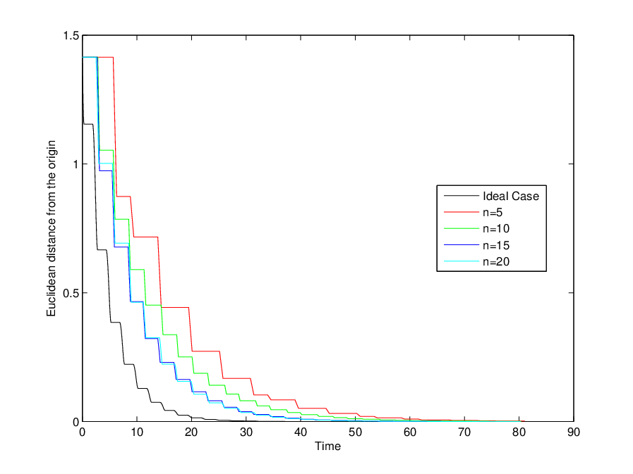
In particular, consider the case where . The coarsest partition of the unit circle that gives rise to a good enough approximate model allowing for successful control design corresponds to . The relevant data for several choices of are shown in Table II, and the implementation of the resulting controllers is plotted in Figure 8, together with the corresponding plot in the “ideal” (full state feedback, unsampled) setting for comparison. Table I explains the significance of the various parameters reported for the examples. In this case, refining the partition by increasing improves both the provable gain bound for and the rate of convergence up to a certain point. The improvement seems to taper off beyond , likely due to numerical errors. Note that while decreases for the cases where and , the actual rate of convergence still improves as seen in the simulations, thus reinforcing the fact that the actual rate of convergence may be significantly better than the provable rate.
| 5 | 39 | 0.6283 | 0.75 | 0.0160 | 10 |
| 10 | 107 | 0.3142 | 0.625 | 0.0267 | 20 |
| 15 | 207 | 0.2094 | 0.5833 | 0.0195 | 28 |
| 20 | 331 | 0.1571 | 0.5625 | 0.0152 | 39 |
Example 5.9.
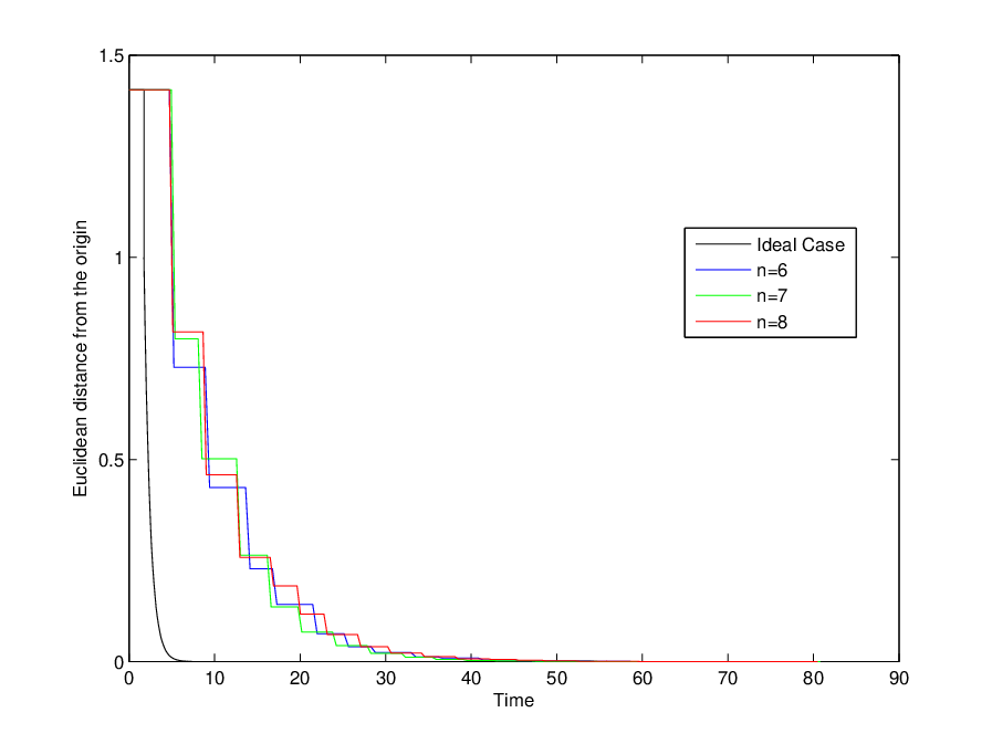
Now consider the case where . In this case, the coarsest workable partition of the unit circle giving rise to a good enough approximate model allowing for successful control design corresponds to . The relevant data for several choices of are shown in Table III, and the implementation of the resulting controllers is plotted in Figure 9, together with the corresponding plot in the “ideal” setting for comparison. Note in this case that even though the best provable gain bound for the error system remains unchanged between and , the difference between and decreases as the unit circle partition is refined, hence the quality of approximation effectively improves as does the guaranteed rate of convergence. Also note that in this case the improvement stalls much sooner, around . This is likely due to the fact that the “aggressive” control law is much more aggressive than in the previous example, and hence numerical errors affect the computation sooner.
| 6 | 39 | 0.5236 | 1 | 0.0141 | 11 |
| 7 | 55 | 0.4488 | 1 | 0.0387 | 13 |
| 8 | 69 | 0.3927 | 1 | 0.0279 | 17 |
6 CONCLUSIONS AND FUTURE WORK
A new constructive approach for designing switching controllers to stabilize pairs of discrete-time homogenous second order systems under limited information (due to binary sensors) was presented. The hybrid plant is first approximated by a deterministic finite state machine, and a useable description of the resulting approximation error, in the form of a ”gain” bound, is established. Using a ”small gain” argument and dynamic programming techniques, a controller is then synthesized to robustly stabilize the nominal (approximate) model in the presence of admissible (approximation) uncertainty. The resulting stabilizing controller then consists of a deterministic finite state machine observer for the hybrid plant and a corresponding full state feedback switching law. While the proposed approach is inspired from classical robust control, the use of deterministic finite state machines as an alternative class of nominal models necessitates the development of a new set of complementary approximation, analysis and control tools.
Future work will focus on three main directions:
- 1.
Reducing the conservatism of the approach: As mentioned in the paper, the proposed approach for computing gain bounds for the approximation uncertainty is efficient (polynomial in the size of the nominal models) but conservative. One direction of future effort will thus focus on developing alternative tractable approaches for verifying tighter gain bounds, allowing for the design of stabilizing controllers with better performance.
- 2.
Extending the approach to broader problems: Another direction of future work will look into extending the proposed analysis, approximation and synthesis tools to broader classes of plants beyond homogeneous systems, in addition to identifying alternative performance objectives (beyond stability) that can be captured by ”gain conditions”.
- 3.
Addressing the issue of scalability: While the design approach presented here can, in principle, be applied to systems of arbitrary order, it scales poorly (exponentially) with plant order, as do most existing hybrid design techniques. Thus one important direction of future work is finding ways of improving the scalability of the approach, potentially by identifying and exploiting system structure.
7 Acknowledgments
The first author was supported by AFOSR Grant FA9550-04-1-0052 while she was at MIT and by startup funds from the Whiting School of Engineering while at The Johns Hopkins University.
8 Proof of Theorem 4.7
Several statements will be useful in proving Theorem 4.7. The first one, Theorem 8.10, is adapted from Theorem 3 in [31] and is presented here without proof.
Theorem 8.10.
Consider a deterministic finite state machine with state transition equation
where is the state set and and are the input sets. Let be a given function. The following two statements are equivalent:
- (a)
The inequality
is satisfied for any and .
- (b)
There exists a non-negative function such that the inequality
holds for all , and .
In the terminology of Willem’s theory of dissipative systems [35], in Theorem 8.10 is the storage function of the dissipative system with supply rate .
Lemma 8.11.
Function defined in (23) is monotonic, that is
Proof 8.12.
When , we have
Thus .
Lemma 8.13.
The sequence defined in (24) is monotonically increasing.
Proof 8.14.
The proof is by induction on . We have
Now suppose . Then
which completes the proof.
Given a scalar and a function , denote by the function from to defined by .
Lemma 8.15.
For any and , .
Proof 8.16.
For any we have
We are now ready to prove Theorem 4.7.
Proof 8.17.
(Theorem 4.7)
(b) (a): Suppose there exists a function
satisfying (22), and let
For any , we have
It follows from Theorem 8.10 that the (deterministic finite state machine) closed loop system satisfies (21).
(a) (c): Suppose there exists a such that the closed loop system satisfies (21). By Theorem 8.10, there exists a such that
We then have
It follows that function also satisfies
for any choice of . Since the set is finite, we can assume, without loss of generality, that with and .
References
- [1] R. K. Ahuja, T. L. Magnanti, and J. B. Orlin, Network Flows: Theory, Algorithms and Applications. Prentice Hall, 1993.
- [2] R. Alur, T. Henzinger, G. Lafferriere, and G. Pappas, “Discrete abstractions of hybrid systems,” Proceedings of the IEEE, vol. 88, no. 2, pp. 971–984, 2000.
- [3] R. E. Bellman, Dynamic Programming. Princeton, New Jersey: Princeton University Press, 1957.
- [4] C. Benassi and A. Gavioli, “Hybrid stabilization of planar linear systems with one-dimensional outputs,” Systems and Control Letters, vol. 46, pp. 303–309, 2002.
- [5] D. P. Bertsekas, Dynamic Programming and Optimal Control, 2nd ed. Belmont, Massachusetts: Athena Scientific, 2000, vol. 1.
- [6] J. Daafouz, P. Riedinger, and C. Iung, “Stability analyis and control synthesis for switched systems: A switched lyapunov function approach,” IEEE Transactions on Automatic Control, vol. 47, no. 11, pp. 1883–1887, 2002.
- [7] R. DeCarlo, M. Branicky, S. Pettersson, and B. Lennarston, “Perspectives and results on the stability and stabilizability of hybrid systems,” Proceedings of the IEEE, vol. 88, no. 7, pp. 1069–1082, July 2000.
- [8] E. Feron, “Quadratic stabilizability of switched systems via state and output feedback,” MIT Center for Intelligent Control Systems, Tech. Rep. CICS-P-468, 1996.
- [9] A. F. Filippov, “Stability conditions in homogeneous systems with arbitrary regime switching,” Automation and Remote Control, vol. 41, pp. 1078–1085, 1980.
- [10] A. Girard and G. Pappas, “Approximation metrics for discrete and continuous systems,” IEEE Transactions on Automatic Control, vol. 52, no. 5, pp. 782–798, 2007.
- [11] T. A. Henzinger, P. W. Kopke, A. Puri, and P. Varaiya, “What’s decidable about hybrid automata,” Journal of Computer and System Sciences, vol. 57, no. 1, pp. 94–124, 1998.
- [12] D. Holcman and M. Margaliot, “Stability analysis of second -order switched homogeneous systems,” SIAM Journal on Control and Optimization, vol. 41, no. 5, pp. 1609–1625, 2003.
- [13] J. Y. Hung, W. Gao, and J. C. Hung, “Variable structure control: A survey,” IEEE Transactions on Industrial Electronics, vol. 40, no. 1, pp. 2–22, February 1993.
- [14] H. K. Khalil, Nonlinear Systems, 3rd ed. New Jersey: Prentice Hall, 2002.
- [15] G. Lafferriere, G. J. Pappas, and S. Sastry, “O-minimal hybrid systems,” Mathematics of Control, Signals and Systems, vol. 13, no. 1, pp. 1–21, 2000.
- [16] M. V. Lawson, Finite Automata. CRC Press, 2004.
- [17] D. Liberzon, Switching in Systems and Control, ser. Systems and Control: Foundations and Applications. Boston, MA: Birkhauser, June 2003.
- [18] H. Lin and P. Antsaklis, “Stability and stabilizability of switched linear systems: A survey of recent results,” IEEE Transactions on Automatic Control, vol. 54, no. 2, pp. 308–322, February 2009.
- [19] J. Lunze, “Qualitative modeling of linear dynamical systems with quantized state measurements,” Automatica, vol. 30, pp. 417–431, 1994.
- [20] A. Megretski, “Robustness of finite state automata,” in Multidisciplinary Research in Control: The Mohammed Dahleh Symposium 2002, ser. Lecture Notes in Control and Information Sciences, L. Giarre and B. Bamieh, Eds. Berlin; New York: Springer, 2003, no. 289, pp. 147–160.
- [21] J. Raisch and S. D. O’Young, “Discrete approximation and supervisory control of continuous systems,” IEEE Transactions on Automatic Control, vol. 43, no. 4, pp. 569–573, April 1998.
- [22] P. J. G. Ramadge and W. M. Wonham, “The control of discrete event systems,” Proceedings of the IEEE, vol. 77, no. 1, pp. 81–98, January 1989.
- [23] K. R. Santarelli, A. Megretski, and M. A. Dahleh, “Stabilizability of two-dimensional linear systems via switched ouput feedback,” Systems & Control Letters, vol. 57, pp. 228–235, 2008.
- [24] R. Shorten, F. Wirth, O. Mason, K. Wulff, and C. King, “Stability criteria for switched and hybrid systems,” SIAM Review, vol. 49, no. 4, pp. 545–592, 2007.
- [25] P. Tabuada, “An approximate simulation approach to symbolic control,” IEEE Transactions on Automatic Control, vol. 53, no. 6, pp. 1406–1418, July 2008.
- [26] P. Tabuada, A. Ames, A. Agung, and G. Pappas, “Approximate reduction of dynamical systems,” Systems & Control Letters, vol. 7, no. 57, pp. 538–545, 2008.
- [27] P. Tabuada, Verification and Control of Hybrid Systems: A Symbolic Approach. Springer, 2009.
- [28] D. C. Tarraf, “A finite state machine framework for robust analysis and control of hybrid systems,” PhD Dissertation, Massachusetts Institute of Technology, Department of Mechanical Engineering, June 2006.
- [29] D. C. Tarraf, A. Megretski, and M. A. Dahleh, “On stabilizing the double integrator with switched gain feedback and binary sensing,” in Proceedings of the Forty-Fourth Annual Allerton Conference on Communication, Control and Computing, Allerton, Il, October 2006, pp. 160–168.
- [30] ——, “Finite state controllers for stabilizing switched systems with binary sensors,” in Hybrid Systems: Computation and Control, ser. Lecture Notes in Computer Science, A. Bemporad, A. Bicchi, and G. C. Buttazzo, Eds. Springer, 2007, vol. 4416, pp. 543–556.
- [31] ——, “A framework for robust stability of systems over finite alphabets,” IEEE Transactions on Automatic Control, vol. 53, no. 5, pp. 1133–1146, 2008.
- [32] D. C. Tarraf, A. Megretski, and M. Dahleh, “Finite automata approximations with error bounds for systems with quantized actuation and measurement: A case study,” in Proceedings of the Conference on Decision and Control, Paradise Island, Bahamas, December 2004, pp. 1436–1441.
- [33] M. Vidyasagar, Nonlinear Systems Analysis, 2nd ed., ser. Classics in Applied Mathematics. SIAM, 2002.
- [34] M. Wicks, P. Peleties, and R. DeCarlo, “Switched controller synthesis for the quadratic stabilization of a pair of unstable linear systems,” European Journal of Control, vol. 4, pp. 140–147, 1998.
- [35] J. C. Willems, “Dissipative dynamical systems - Part I: General theory,” Archive for Rotational Mechanics and Analysis, vol. 45, pp. 321–351, 1972.